Transverse Spin Structure Function in the Valon model
Abstract
The spin dependent structure function, , is calculated in the valon model. A simple approach is given for the determination of the twist-3 part of the in Mellin space; thus, enabling us to obtain the full transverse structure function, for proton, neutron and the deuteron. In light of the new data, we have further calculated the transversely polarized structure function of . Our results are checked against the experimental data and nice agreements are observed.
1 INTRODUCTION
The nucleon polarized structure functions are
important tools in understanding the nucleon substructure. In
particular, they are indispensable elements for the understanding
of the spin dependent parton distributions and their correlations.
The structure function is important because it
probes transversely and also longitudinally polarized parton
distributions inside the nucleon. structure
function is also sensitive to the higher twist effects, such as
quark gluon correlations. They do not disappear even at large
values and not easily interpreted in pQCD
[1, 2]. Since is the only
function related to the quark-gluon interaction, learning
about its behavior will render further insight into the spin structure of the nucleon beyond the simple quark parton model.
Thus, the main purpose of this paper is to calculate transverse spin structure function,
. As such, it requires considering both the twist-2 and the twist-3 contributions.
Here we will present a simple method to extract twist-3 part. The twist-2 part is
well understood, and requires knowledge about the structure function.
Therefore, first we will briefly review in the context of the so called valon model representation of hadrons.
Finally, the outcome of our results is checked against the
experimental data from
[3, 4, 5, 6, 7], and compared with other phenomenological models.
The lay out of the paper is as follows: In section 2, we briefly
present a review of the polarized nucleon structure function in
the valon model. Section 3 deals with the calculation of
spin structure function and discusses the numerical
results. We also provide some discussion on the effect of higher twists. Section 4 is devoted to the sum rules. Our conclusions are given in section 5.
2 A brief review of spin structure functions in the valon model
The valon model is a phenomenological model, originally proposed
by R. C. Hwa, [8] in early 80’s to provide a bridge
between the naive quark model and the partonic structure of the
hadrons. The model had many successes. It was improved later by
Hwa [9] and Others
[10, 11, 12, 13, 14, 15]. It was
further extended to include the polarized cases [16, 17, 18, 19]. The model views a hadron as three
(two) constituent quark like objects called valons. Each valon is
defined to be a dressed valence quark with its own cloud of sea
quarks and gluons. The dressing processes are
described by QCD. At high enough values the structure of a valon can be resolved, but At low values, the internal structure of the valon cannot be resolved and it behave as a constituent quarks of the hadron.
In valon model the polarized parton distributions of a polarized
hadron are given by the following convolution integral :
| (1) |
where is the valon helicity distribution in the hosting hadron; that is, it is the probability of finding a polarized valon inside the polarized hadron. In the Next-to-Leading order, marginally depends on . These distributions are shown in (Fig.1).

The term in Eq.(1) is the polarized parton distribution (PPDFs) inside a valon and are obtained from the solutions of DGLAP evolution equations in the valon. Now, using the convolution integral, one can obtain the polarized hadron structure functions as follows:
| (2) |
where is the polarized structure function of the valon. The details of actual calculations are given in [16, 18]. In short, the following two steps lead us to both the polarized PPDFs and polarized nucleon structure functions:
- •
Calculate the PPDFs in the valon using DGLAP equations;
- •
It should be noted that the valon model is only a phenomenological model. As such, initial conditions, as inputs to the DGLAP equations, are chosen based on phenomenological arguments. The results obtained for the proton structure function, from this model are in excellent agreement with all available experimental data [20, 21, 22, 23, 24, 25]. In Fig.2 we only present a sample of the results along with the existing data. The parton distributions so obtained will be used here to calculate .


3 Transverse spin-dependent structure function
Polarized Deep Inelastic Scattering (DIS) mediated by a photon exchange, probes two spin structure functions: and . If the target is transversely polarized, the total cross section is a combination of these two structure functions. Transverse spin structure function, , is made up of two components: a twist-2 part, , and a mixed twist part, . Therefore, it can be written as [26]:
| (3) |
where
| (4) |
The twist-2 part, , comes from OPE. The receives a contribution from the transversely polarized
quark distributions plus a contribution that
comes from a twist-3 component, an indication of correlations, given by
term in Eq.(4). These higher
twist corrections arise from the non-perturbative multi parton
interactions. Their contributions at low energy increase as , reflecting the confinement. Any non-zero result for
this term at a given will reflect a departure from the
non-interacting partonic regime [27].
is related to the structure function by the
Wandzura-Wilczek relation [28] as follows,
| (5) |
3.1 Calculation of the twist-2 term,
We begin with Eq.(5). Since is known in the valon model [16, 18], we utilize them without any additional free parameter and evaluate the twist-2 part of ; namely , according to the Eq.(5). The results are shown in Fig. 3 for proton. We have also included the findings of [29, 30] for the purpose of comparison.

3.2 Calculating the twist-3 term,
As mentioned, the function has two
terms. The first term is a twist-2 contribution related to the
transverse polarization of quarks in the nucleon. It is suppressed
by the quark to nucleon mass ratio and will be ignored here due to
its negligibility. The second part is a twist-3 contribution, reflecting
the quark-gluon correlations. In the following we will focus on this part.
In large limit, Ali, Braun and Hiller found that the
-evolution of is qualified by simple
DGLAP type equation with awhile difference between the anomalous
dimensions and the twist-2 distribution[31, 32]. It implies that
obeys the following simple equation :
| (6) |
where,
| (7) |
| (8) |
and
| (9) | |||
| (10) | |||
| (11) |
is the strong coupling constant, is the number
of flavor and are the Harmonic functions. Our purpose is
to find the -evolution of with some appropriate
initial conditions in moment space. Then we can make a
transformation to the momentum space and evaluate the twist-3
contribution to the transverse spin structure function. This is
done in two steps, as is the case in the valon model. The first
step involves finding a solution to Eq.(6) in a valon.
The second step is to convolute the results obtained in the first
step with the valon distribution in the nucleon. This will give
the nucleon structure function.
We take as our initial scale which is also
used in our original calculations of various parton distributions.
This value of corresponds to a distance scale of which is roughly equal to or less than the radius of a
valon[11]. The initial input function for is (See the Appendix A) :
| (12) |
The justification for this choice is as following: In the momentum space one can write
| (13) |
Note that for we get which is apparent from the definition of in Eq.(8), thus, arriving at Eq.(12). This simple choice for the initial input in stems from the knowledge that it is related to the quark gluon correlations, which in turn, is related to the Green function in the momentum space. In the momentum space the correlation function is composed of a Dirac Delta term and a function that is related to the momentum. consequently, at the initial we can simply assume that is proportional to Dirac Delta function which emphasizes the conservation of energy- momentum and the fact that at such a low a valon behaves as an object without any internal structure. The last point is built in the definition of a valon. So, in the moment space the Delta function becomes unity and we can write
| (14) |
all of the QCD effects are summarized in . This coefficient will be extracted from the experimental data. A fit to E143 data yeilds a value for A. Having specified the initial input values, the moments of in a valon are readily obtained, with the aid of Eq.(14). An inverse Mellin transformation then takes us to the momentum space, giving structure function. For example at , we have:
| (15) |
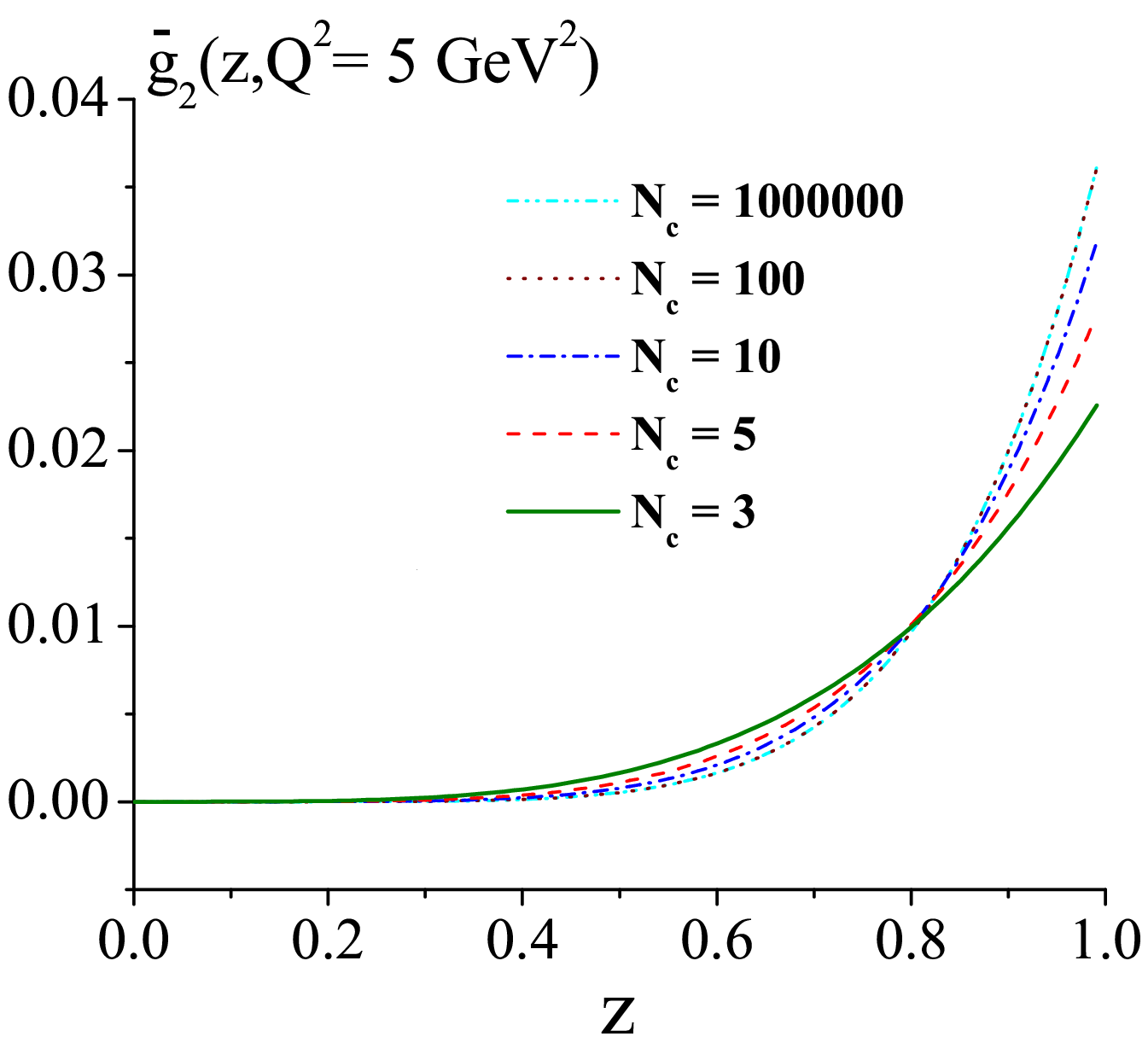
This completes the first step described above. In Fig.4, is shown for different values of . According to Fig.5 as our calculations for the values of leads to a similar distribution for for the whole range of , We are choosing the optimal value of which is equal to (reminder that Eq. (6) is valid only for large ).

The second step involves the convolution process which takes us to the hadronic level. This is similar to the earlier procedure that we have used to extract . Similar to , we can write:
| (16) |
where is the transverse valon
distribution functions describing the probability of finding a
valon with spin aligned or anti-aligned with the transversly
polarized proton. In fact, is
identical to in the longitudinal
case. This is so, because we know that in the non-relativistic
limit of the quark motion, the PPDFs and transversity distribution
would be identical, since the rotations and Euclidean boosts
commute and a series of boosts and rotation can convert a
longitudinal polarized proton into a transversely polarized one
with an infinite momentum [33, 34, 35].
Finally substituting the valon helicity distribution, in the corresponding hadron leads us to . In Fig.6 we present for both
proton and deuteron along with the E143 data [3] . We have
compared our results
with those obtained in the Bag model [29] and that of Wakamatsu [32].


Finally, adding and , gives the full . The final results for are presented in Fig.7 for proton, neutron and deuteron at different values of .


Confronting with the experimental data, in Fig.8 we show our results for the full transversely polarized structure function for proton, neutron and deuteron and the experimental findings of [3, 4, 6].


3.3 The case of
It is intriguing to investigate
the as a special case, since there are
some newly released data on , and the
conformity of our result with the experiment will lend further
justification to the approach adopted here.
The structure function can be viewed as the sum of and , each convoluted with the spin dependent nucleon light-cone momentum distributions, , where is the ration of ” components of the light cone momenta of struck nucleon to nucleus. One will have
| (17) |
So, using Eq.(17), this should be straightforward. All is needed are two functions, namely, and . They can be extracted from the numerical results of [36, 37]. In Fig. 9 we have plotted together with the experimental data from [38, 39, 40].

As can be seen from the figure, our approach is in fair agreement with the experimental data.
4 The Sum Rules
There are two important and well known sum rules regarding and . The first one is OPE sum rule:
| (18) |
| (19) |
where and are the twist-2 and the twist-3 matrix
element operators, respectively. The study of these sum rules is
easy for simplest case (n=2) where the twist three effects are
exist [1, 2].
The second one is the Burkhardt-
Cottingham sum rule [41]. It states that the first
moment of structure function vanished.
| (20) |
Since , upon combining Eq. (18) and Eq. (19) with Eq. (5) provides a third sum rule. They are listed bellow:
| (21) | |||
| (22) | |||
| (23) |
we have evaluated in the valon model for a number of values, the results are shown in Fig. 10 and compared with the available data, the bag model, and the QCD Sum Rule results. Table 3 shows our results for the Burkhardt-Cottingham sum rule in the region at . They are checked against the data from HERMES in the same region and also with the findings of E143 and E155 in the range . For the purpose of comparison, results from other sources are also included. While is in excellent agreement with the experiment, is less so. However, we also notice that there are fewer data for and thus, making it difficult to arrive in a firm conclusion.
Valon model 0.01956 -0.00004 0.00874 Lattice QCD [45] CM bag model by Song [29] E143 [3]
Valon model 0.00519 0.0042 0.00437 MIT bag model [29, 42] QCD sum rule [43] QCD sum rule [44] Lattice QCD [45] CM bag model by Song [29] E143 [3]


bag model by Song[29] E143 E155 HERMES 2012 Valon model -0.0016 -0.0016 -0.00287 — - 0.0092
5 Conclusion
We have used the so-called valon model to calculate the transverse spin structure functions of the nucleon and the deuteron. To do so, we provide a simple approach for calculating the twist-3 part of the transverse spin structure function in Mellin space. Furthermore, as a separate check on the validity of our approach, we have considered , where we have utilized some light cone momentum distribution and compared with the new data from [40]. Evidently our findings are in agreement with the experiment, rendering the conclusion that hadronic structure functions, both polarized and unpolarized, are nicely described in the valon representation.
Appendix
Here we attempt to justify our choice of initial input value in :
As we know the is related to quark-gluon-quark
correlation. Since, by definition, at initial scale, , the
valon behaves as an object with no internal structure,
it is reasonable to assume that, at such initial scale this object is related to the
quark-quark correlations(two-point green function), because at
such a low gluons carry have very small and negligible momentum.
The general form of two-point green function in momentum space is
given here (Eq. (2.102) in [47]):
The structure function is related to the integral over this two-point green function. We don’t know the exact relation between them, but at least we can say that it has two terms: the first one is a function of and the second one is a Dirac Delta function which implies conservation of energy-momentum. To establish this relation, we resort to the phenomenological arguments. Obviously, the simplest choice for is
at initial scale of , the photon probe detects only three valence quarks inside the proton. Hence, we can assume that and we have:
The constant A can be determined from experimental data. Our motivation for this value comes from the phenomenological consideration which is required us to choose the initial input densities as at . This mathematical boundary condition means that the internal structure of the valon cannot be resolved at . At this scale of , the nucleon can be considered as a bound state of three valence quarks that carry all the momentum and the spin of the nucleon. As is increased, other partons can be resolved at the nucleon.
References
- [1] E. Shuryak, A.Vainshtein, Nucl. Phys. B 201, 141 (1982)
- [2] E. Shuryak, A.Vainshtein, Phys.Lett. B105 (1981) 65-67
- [3] Abe et al. (E143 Colaboration), Phys. Rev. D 58, 112003 (1998)
- [4] Anthony et al. (E155 Collaboration), Phys. Lett. B 458, 529535 (1999); Phys. Lett. B 553, 18 (2003)
- [5] Peter E. Bosted, (E155x Collaboration), RIKEN Review No. 28 (2000)
- [6] V. A. Korotkov (HERMES Collaboration), PoS DIS 2010: 234, (2010)
- [7] A. Airapetian et al. Eur. Phys. J. C 72, 1921 (2012)
- [8] R. C. Hwa, Phys. Rev. D 22, 759 (1980)
- [9] R. C. Hwa and C. B. Yang, Phys. Rev. C 66, 025205 (2002)
- [10] G. Altarelli, S. Petrarca and F. Rapuano, Phys. Lett. B 373, (1996) 200 [hep-ph/9510346].
- [11] F. Arash and A. N. Khorramian, Phys. Rev. C 67, 045201 (2003) [hep-ph/0303031].
- [12] F. Arash, Phys. Lett. B 557, 38 (2003) [hep-ph/0301260].
- [13] F. Arash, Phys. Rev. D 69, 054024 (2004) [hep-ph/0307221].
- [14] F. Arash, Phys. Rev. D 50, 1946 (1994).
- [15] F. Arash, Phys. Rev. D 52, 68-71 (1995).
- [16] F. Arash, F. Taghavi Shahri, JHEP 07, 071 (2007)
- [17] F. Arash, F.Taghavi Shahri, Phys. Lett. B 668, 193(2008)
- [18] F. Taghavi Shahri, F. Arash, Phys. Rev. C 82, 035205 (2010)
- [19] A. Shahveh, F. Taghavi Shahri, F. Arash, Phys. Lett B 691, 32-36 (2010)
- [20] M. G. Alekseev (COMPASS Collaboration), Phys. Lett. B 690, 466 (2010)
- [21] A. Airapetian et al. Phys. Rev. D 75, 012007 (2007) [hep-ex/0609039]
- [22] V. Yu. Alexakhin et al. (COMPASS Collaboration), Phys. Lett. B 647, 8-17 (2007) [hep-ex/0609038]
- [23] K. Kramer,et al. Phys. Rev. Lett 95, 142002 (2005) [nucl-ex/0506005]
- [24] K. Abe, et al. Phys. Lett. B 405, 180-190 (1997); Phys. Rev. Lett. 79 26 (1997)
- [25] K. Abe, et al. (E143 Collaboration), Phys. Rev. Lett 75, 25 (1995); Phys. Rev. Lett. 78, 815 (1997)
- [26] J. L. Cortes, B. Pire, J. P. Ralston, Z. Phys. C 55, 409 (1992)
- [27] K. Slifer et al. (RSS Collaboration), Phys. Rev. Lett 105, 101601 (2010)
- [28] S. Wandzura, F. Wilczek, Phys. Lett. B 72, 195 (1977)
- [29] X. Song, Phys. Rev. D 54, 1955 (1996)
- [30] X. Song, Phys. Rev. D 63, 094019 (2001)
- [31] A. Ali, V. M. Brauun, G.Hiller, Phys. Lett. B 266, 117 (1991)
- [32] M. Wakamatsu, Phys. Lett. B 487, 118-124 (2000)
- [33] Z. Alizadeh Yazdi, F. Taghavi-Shahri, F. Arash and M. E. Zomorrodian, Phys. Rev. C 89, 055201 (2014)
- [34] M. Anselmino, M. Boglione, U. D’Alesio, A. Kotzinian, S. Melis, F. Murgia and A. Prokudin, Nucl. Phys. Proc. Suppl. 191 (2009) 98–107, [hep-ph/0812.4366]
- [35] V. Barone, F. Bradamantec, A. Martin, Progress in Particle and Nuclear Physics 65 (2010) 267-333
- [36] F. R. P. Bissey, A. W. Thomas, I. R. Afnan, Phys. Rev. C 64, 024004 (2001); F. R. P. Bissey, V. A. Guzey, M. Strikman, A.W. Thomas, Phys. Rev. C 65, 064317 (2002); I. R. Afnan, et al., Phys. Rev. C 68, 035201 (2003)
- [37] M. M. Yazdanpanah, A. Mirjalili, S. Atashbar Tehrani, F. Taghavi Shahri, Nucl. Phys. A 831, 243-262 (2009)
- [38] Anthony et al. (E142 Collaboration), Phys. Rev. D 54, 6620 (1996)
- [39] X. Zheng et al. (The Jefferson Lab Hall A Collaboration ), Phys. Rev. C 70, 065207 (2004)
- [40] M. Posik et al. (The Jefferson Lab Hall A Collaboration ), Phys. Rev. Lett 113, 022002 (2014)
- [41] H. Burkhardt and W. N. Cottingham, Ann. Phys. 56, 453 (1970)
- [42] X. Ji, P. Unrau, Phys. Lett. B 333, 228 (1994)
- [43] E. Stein, Phys. Lett. B 343, 369 (1995)
- [44] I. Balitsky, V. Braun, A. Klesnichenko, Phys. Lett. B 242, 1990
- [45] M. Gockeler et al. Phys. Rev. D 53, 2317 (1996)
- [46] M. Osipko et al. Phys. Rev. D 71, 054007 (2005)
- [47] Stefan pokorski,” Gauge field theories ”, Cambridge University press, (2000)