Periodic travelling waves and compactons in granular chains

Guillaume James Address: Laboratoire Jean Kuntzmann, Université de Grenoble and CNRS, BP 53
38041 Grenoble Cedex 9, France. Email address: Guillaume.James@imag.fr

Date: August 24, 2026

Abstract.

We study the propagation of an unusual type of periodic travelling waves in chains of identical beads interacting via Hertz’s contact forces. Each bead periodically undergoes a compression phase followed by a free flight, due to special properties of Hertzian interactions (fully nonlinear under compression and vanishing in the absence of contact). We prove the existence of such waves close to binary oscillations, and numerically continue these solutions when their wavelength is increased. In the long wave limit, we observe their convergence towards shock profiles consisting of small compression regions close to solitary waves, alternating with large domains of free flight where bead velocities are small. We give formal arguments to justify this asymptotic behaviour, using a matching technique and previous results concerning solitary wave solutions. The numerical finding of such waves implies the existence of compactons, i.e. compactly supported compression waves propagating at a constant velocity, depending on the amplitude and width of the wave. The beads are stationary and separated by equal gaps outside the wave, and each bead reached by the wave is shifted by a finite distance during a finite time interval. Below a critical wavenumber, we observe fast instabilities of the periodic travelling waves leading to a disordered regime.

Key words and phrases:

Granular chain, Hertzian contact, Hamiltonian lattice, periodic travelling wave, compacton, fully nonlinear dispersion.

2000 Mathematics Subject Classification

37K60, 70F45, 70K50, 70K75, 74J30

Laboratoire Jean Kuntzmann,

Université de Grenoble and CNRS,

BP 53, 38041 Grenoble Cedex 9, France.

1. Introduction and main results

Understanding wave propagation in granular media is a fundamental issue in many contexts, e.g. to design shock absorbers [44, 18], derive multiple impact laws [25, 3, 35, 33, 34], detect buried objects by acoustic sensing [45], or understand possible dynamical mechanisms of earthquake triggering [32]. One of the important factors that influence wave propagation is the nature of elastic interactions between grains. According to Hertz’s theory, the repulsive force $f$ between two identical initially tangent spherical beads compressed with a small relative displacement $\delta$ is $f(\delta)=k\,\delta^{\alpha}$ at leading order in $\delta$ , where $k$ depends on the ball radius and material properties and $\alpha=3/2$ (see figure 1). This result remains valid for much more general geometries (smooth non-conforming surfaces), and $\alpha$ can be even larger in the presence of irregular contacts [31, 22]. The Hertz contact force has several properties that make the analytical study of wave propagation more difficult than in classical systems of interacting particles : the dependency of $f(\delta)$ on $\delta\approx 0$ is fully nonlinear for $\alpha>1$ , $f^{\prime\prime}(0)$ is not defined for $\alpha<2$ , and no force is present when beads are not in contact. This makes the use of perturbative methods rather delicate, since the latter often rely on nonlinear modulation of linear waves which are not present in such systems, and usually require higher regularity of nonlinear terms.

Refer to caption — Figure 1. Schematic representation of two identical and initially tangent spherical beads that are compressed and slightly flatten, the distance between their centers decreasing by $\delta\approx 0$ .

The simplest model in which these difficulties show up consists of a line of identical spherical beads, in contact with their neighbours at a single point when the chain is at rest. For an infinite chain of beads, the dynamical equations read in dimensionless form

\frac{d^{2}x_{n}}{dt^{2}}=V^{\prime}(x_{n+1}-x_{n})-V^{\prime}(x_{n}-x_{n-1}),\ \ \ n\in\mathbb{Z},

(1)

where $x_{n}(t)\in\mathbb{R}$ is the displacement of the $n$ th bead from a reference position and the interaction potential $V$ corresponds to Hertz contact forces. It takes the form

V(x)=\frac{1}{1+\alpha}\,|x|^{1+\alpha}\,H(-x),

(2)

where $H$ denotes the Heaviside function vanishing on $\mathbb{R}^{-}$ and equal to unity on $\mathbb{R}^{+}$ and $\alpha>1$ is a fixed constant. System (2) is Hamiltonian with total energy

{\mathcal{H}}=\sum_{n\in\mathbb{Z}}{\frac{1}{2}\,(\frac{dx_{n}}{dt})^{2}+V(x_{n+1}-x_{n})}.

(3)

For $\alpha=3/2$ , Nesterenko analyzed the propagation of compression pulses in this system using a formal continuum limit and found approximate soliton solutions with compact support [37, 38] (see also [4, 40, 44] for more recent results and references). As shown by MacKay [36] (see also [30]), exact solitary wave solutions of (1) exist since an existence theorem of Friesecke and Wattis [21] can be applied to the chain of beads with Hertz contact forces (see also [48] for an alternate proof). Moreover these solitary waves have in fact a doubly-exponential decay [9, 15, 48] that was approximated by a compact support in Nesterenko’s analysis.

Much more analytical results are available on nonlinear waves in the granular chain when an external load $f_{0}$ is applied at both ends and all beads undergo a small compression $\delta_{0}$ when the system is at rest. Around this new equilibrium state, the dynamical equations correspond to a Fermi-Pasta-Ulam (FPU) lattice [7, 23, 39], that sustains in particular stable solitary waves with exponential decay (see e.g. [21, 19, 27, 20, 26]) and periodic travelling waves also known as “nonlinear phonons” [17, 27, 13, 39, 24]. The existence and qualitative properties of periodic travelling waves in granular chains are important elements in the understanding of energy propagation and dispersive shocks in these systems, as shown in reference [14] in the similar context of FPU lattices. However, the persistence of periodic travelling waves when $f_{0}\rightarrow 0$ is not obvious because the sound velocity (i.e. the maximal velocity of linear waves) vanishes as $f_{0}^{1/6}$ , and the uncompressed chain of beads is commonly denoted as a “sonic vacuum” [38].

In this paper we show that periodic travelling waves with unusual properties exist in granular chains under Hertz contacts without precompression. These waves consist of packets of compressed beads alternating with packets of uninteracting ones, so that any given bead periodically switches between a free flight regime and a contact regime where it interacts nonlinearly with two or one neighbours. Waves of this type have been numerically computed in reference [47], for periodic granular chains consisting of three or four beads. Here we provide an existence theorem valid at wavenumbers close to $\pi$ and proceed by numerical continuation when the wavenumber goes from $\pi$ to the long wave limit $q\rightarrow 0$ . The limit $q=\pi$ corresponds to binary oscillations, i.e. travelling waves with spatial period $2$ where nearest neighbours oscillate out of phase. In the long wave limit, the periodic waves display small compression regions close to solitary waves, alternating with large domains of free flight where bead velocities are small.

Our existence result for periodic travelling waves close to binary oscillations is described in the following theorem. In what follows, $C^{k}_{\rm{per}}(0,2\pi)$ denotes the classical Banach space of $2\pi$ -periodic and $C^{k}$ functions $u\,:\mathbb{R}\rightarrow\mathbb{R}$ , endowed with the usual supremum norm taking into account all derivatives of $u$ up to order $k$ .

Theorem 1.

System (1) with interaction potential (2) admits two-parameter families of periodic travelling wave solutions

x_{n}^{\pm}(t;a,\mu)=a\,u_{\mu}[(\pi+\mu)\,n\pm a^{\frac{\alpha-1}{2}}t],

(4)

parametrized by $a>0$ and $\mu\in{\mathcal{V}}$ , where ${\mathcal{V}}$ denotes an open interval containing $0$ . The function $u_{\mu}$ is odd, $2\pi$ -periodic and satisfies the advance-delay differential equation

u_{\mu}^{\prime\prime}(\xi)=V^{\prime}(u_{\mu}(\xi+\pi+\mu)-u_{\mu}(\xi))-V^{\prime}(u_{\mu}(\xi)-u_{\mu}(\xi-\pi-\mu)).

(5)

The map $\mu\mapsto u_{\mu}$ belongs to $C^{1}({\mathcal{V}},C^{2}_{\rm{per}}(0,2\pi))$ and satisfies the symmetry property $u_{\mu}(\xi)=-u_{-\mu}(\xi+\pi)$ . The function $u_{0}$ is determined by the initial value problem

u_{0}^{\prime\prime}+W^{\prime}(u_{0})=0,

(6)

u_{0}(0)=0,\ \ \ u_{0}^{\prime}(0)=p_{0},\ \ \ p_{0}=(1+\alpha)^{\frac{\alpha}{1-\alpha}}\Big[\frac{\sqrt{\pi}\,\Gamma{(\frac{1}{1+\alpha}+\frac{1}{2})}}{\Gamma{(\frac{1}{1+\alpha})}}\Big]^{\frac{1+\alpha}{1-\alpha}},

(7)

where $W(x)=\frac{2^{\alpha}}{1+\alpha}|x|^{1+\alpha}$ is a symmetrized Hertz potential and $\Gamma{(x)}=\int_{0}^{+\infty}{e^{-t}\,t^{x-1}\,dt}$ denotes Euler’s Gamma function. Moreover, for $\mu<0$ , $u_{\mu}$ is a linear function of $\xi$ on an interval $[-\xi_{1}(\mu),\xi_{1}(\mu)]$ with $\xi_{1}(\mu)=|\mu|/2+o(\mu)$ . It takes the form

u_{\mu}(\xi)=p_{\mu}\,\xi\mbox{ for all }\xi\in[-\xi_{1}(\mu),\xi_{1}(\mu)],

(8)

with $p_{\mu}=p_{0}+O(|\mu|)$ . When $\xi=(\pi+\mu)\,n\pm a^{\frac{\alpha-1}{2}}t\in(-\xi_{1}(\mu)+2k\pi,\xi_{1}(\mu)+2k\pi)$ ( $k\in\mathbb{Z}$ ), the $n$ th particle performs a free flight characterized by

x_{n+1}^{\pm}(t;a,\mu)>x_{n}^{\pm}(t;a,\mu),\ \ \ x_{n}^{\pm}(t;a,\mu)>x_{n-1}^{\pm}(t;a,\mu),\ \ \ \dot{x}_{n}^{\pm}(t;a,\mu)=\pm a^{\frac{\alpha+1}{2}}\,p_{\mu}.

To prove theorem 1, we locally solve equation (5) using the implicit function theorem, where we have to pay a particular attention to regularity issues due to the limited smoothness of the interaction potential $V$ . This approach is reminiscent of the previous work [28], where we proved the existence of periodic travelling waves in the Newton’s cradle, a mechanical system in which the granular chain is modified by attaching each bead to a local linear pendulum. However, in that case the periodic travelling waves were obtained by nonlinear modulation of linear oscillations in the local potentials, a limit which does not exist in the present situation.

A complementary approach to the analysis of exact periodic travelling waves consists of obtaining approximate solutions described by continuum models. Approximate periodic travelling waves have been previously studied through a formal continuum limit in the granular chain (see [38], sections 1.3-5, [16], section 4.6 and references therein), but in a case where all beads were interacting under compression. Closer to our case, Whitham’s modulation equation may be used to approximate the solutions of theorem 1 and study their stability properties, following the lines of reference [13] where the example of a granular chain with linear contact interactions was analyzed.

A limitation of theorem 1 stems from the fact that it provides an existence result for wavenumbers $q=\pi+\mu$ close to $\pi$ . To analyze the existence of periodic travelling waves on a full range of wavenumbers, we numerically continue (for $\alpha=3/2$ ) the solutions of theorem 1 by decreasing the wavenumber $q$ down to values close to $0$ . We compute the nonlinear dispersion relation associated to periodic travelling waves, and analyze their asymptotic form in the long wave limit $q\approx 0$ . In this limit and when the wave velocity is normalized to unity, one finds large ensembles of beads performing a free flight at small velocity, separated by smaller regions consisting of $4$ - $5$ balls under compression with relative displacements close to a solitary wave. Using a matching technique, we perform a formal asymptotic study of the limit $q\rightarrow 0$ which provides a limiting wave profile in good agreement with our numerical computations.

These results are completed by a stability analysis. We compute the Floquet spectrum modulo shifts of the periodic travelling waves, and find fast linear instabilities below a critical wavenumber $q_{c}\approx 0.9$ . This threshold corresponds to the case when the average number of interacting beads in the compression regions becomes larger or equal to three, or equivalently to the maximal number of adjacent interacting beads becoming $\geq 4$ . In this regime, the initial numerical errors made on the travelling wave profiles are amplified during dynamical simulations, leading to the disappearance of the travelling waves after some transcient time. A disordered regime is established shortly after the instability, but interestingly some partial order can be still observed in the form of intermittent large-scale organized structures. In contrast to the above situation, long-time dynamical simulations of periodic travelling waves with wavenumbers $q>q_{c}$ yield wave profiles that remain practically unchanged when propagating along the lattice. The existence of very slow instabilities in this regime is a more delicate question which will be addressed in a future work.

Besides periodic waves, our numerical results also demonstrate the existence of compactons (solitary waves with compact supports) in chains of beads separated by equal gaps outside the compression wave. For $q\leq q_{k}\approx 1.8$ , the periodic solutions of (5) obtained numerically behave linearly on intervals of length larger than the delay $q=\pi+\mu$ involved in (5), and these solutions can be linearly extended in order to get new solutions of (5). Using this property and the Galilean invariance of (1), we obtain compacton solutions for which the beads are stationary and separated by equal gaps outside the wave, and each bead reached by the wave is shifted by a finite distance during a finite time interval.

Our situation is quite different to what occurs in the absence of gaps between beads, because in that case compactons exist in continuum models of granular chains [37, 38, 4], but a transition from compactons to noncompact (super-exponentially localized) solutions occurs when passing from the continuum model to the discrete lattice [4]. In our case the existence of compactons is linked with the occurence of free flight, made possible by the unilateral character of Hertzian interactions which vanish when beads are not in contact.

The outline of the paper is as follows. In section 2 we prove theorem 1 and study some qualitative properties of the travelling wave profiles. The numerical results are presented in section 3, which contains in addition a formal asymptotic study of the long wave limit and the discussion of the existence of compactons. Section 4 gives a summary of the main results and mentions implications for other works. Lastly, some useful properties of solitary wave solutions are recalled in an appendix.

2. Local continuation of periodic travelling waves

Periodic travelling wave solutions of (1) take the form

x_{n}(t)=u(\xi),\ \ \ \xi=q\,n-\omega\,t,

(9)

where $u$ is $2\pi$ -periodic, $q\in[0,2\pi)$ denotes the wavenumber, $\omega\in\mathbb{R}\setminus\{0\}$ the wave frequency and $\xi\in\mathbb{R}$ the spatial coordinate in a frame moving with the wave. Thanks to a scale invariance of (1), the full set of periodic travelling waves can be deduced from its restriction to $\omega=1$ . Indeed, due to the special form of the Hertz potential (2), any solution $x_{n}$ of (1) generates two families of solutions $x_{n}^{(a)}(t)=a\,x_{n}(\pm\,a^{\frac{\alpha-1}{2}}\,t)$ parametrized by $a>0$ . Consequently, any solution of the form (9) with $\omega=1$ corresponds to two families of periodic travelling waves propagating in opposite directions

x_{n}^{(a)}(t)=a\,u(q\,n\mp a^{\frac{\alpha-1}{2}}t),

(10)

with frequency $\omega=\pm\,a^{\frac{\alpha-1}{2}}$ .

Fixing $\omega=1$ , equation (1) yields the advance-delay differential equation

u^{\prime\prime}(\xi)=V^{\prime}(u(\xi+q)-u(\xi))-V^{\prime}(u(\xi)-u(\xi-q)),\ \ \ \xi\in\mathbb{R},

(11)

with periodic boundary conditions

u(\xi+2\pi)=u(\xi).

(12)

Equation (11) possesses the symmetry $u(\xi)\rightarrow-u({-\xi})$ originating from the reflectional and time-reversal symmetries of (1). In the sequel we restrict our attention to solutions of (11) invariant under this symmetry (i.e. odd in $\xi$ ). This assumption simplifies our continuation procedure, because it eliminates a degeneracy of periodic travelling waves linked with the invariance of (11) under translations and phase-shift.

2.1. Binary oscillations

The following lemma exhibits a particular solution of (11)-(12) obtained for $q=\pi$ and corresponding to binary oscillations in system (1).

Lemma 1.

For $q=\pi$ , there exists an odd solution $u_{0}$ of (11)-(12) determined by the initial value problem (6)-(7), and satisfying

u_{0}(\xi+\pi)=-u_{0}(\xi).

(13)

In addition, there exists a one-parameter family of solutions of (1) taking the form

x_{n}(t)=a\,(-1)^{n+1}\,u_{0}(a^{\frac{\alpha-1}{2}}t),\ \ \ a\in(0,+\infty).

(14)

Proof.

We look for solutions of (11) satisfying (13), so that the advance-delay differential equation reduces to the ordinary differential equation (6) with $W(x)=\frac{1}{2}V(-2|x|)=\frac{2^{\alpha}}{1+\alpha}|x|^{1+\alpha}$ . Now we must find a $2\pi$ -periodic solution $u_{0}$ of (6) satisfying (13). Equation (6) is integrable since $I=\frac{1}{2}(u^{\prime})^{2}+W(u)$ is constant along any solution $u$ , and its phase-space is filled by periodic orbits. Any solution $u$ of (6) with initial condition $u(0)=0$ , $u^{\prime}(0)=p>0$ is odd in $\xi$ (due to the evenness of $W$ ) and its period $T(p)$ is given by

T(p)=4\int_{0}^{u_{\rm{max}}}{(p^{2}-2W(v))^{-1/2}\,dv}

where $u_{\rm{max}}=\frac{1}{2}[p^{2}(1+\alpha)]^{\frac{1}{1+\alpha}}$ . Our aim is to find $p_{0}>0$ such that $T(p_{0})=2\pi$ . Using the change of variable $v=u_{\rm{max}}\,t^{\frac{1}{1+\alpha}}$ , one finds $T(p)=2(1+\alpha)^{\frac{-\alpha}{1+\alpha}}\,\beta\,p^{\frac{1-\alpha}{1+\alpha}}$ , where

\beta=\int_{0}^{1}{t^{\frac{1}{1+\alpha}-1}\,(1-t)^{-1/2}\,dt}=B(\frac{1}{1+\alpha},\frac{1}{2}),

and $B(z,w)=\frac{\Gamma{(z)}\,\Gamma{(w)}}{\Gamma{(z+w)}}$ denotes Euler’s Beta function (see [2], formula 6.2.1 p. 258). Since $\Gamma{(1/2)}=\sqrt{\pi}$ , one obtains finally

T(p)=c_{\alpha}\,p^{\frac{1-\alpha}{1+\alpha}},\ \ \ c_{\alpha}=2\sqrt{\pi}(1+\alpha)^{\frac{-\alpha}{1+\alpha}}\,\frac{\Gamma{(\frac{1}{1+\alpha})}}{\Gamma{(\frac{1}{1+\alpha}+\frac{1}{2})}}.

(15)

Consequently, for $p$ varying in $(0,+\infty)$ the period $T(p)$ is strictly decreasing from $+\infty$ to $0$ , and there exists a unique $p_{0}>0$ such that $T(p_{0})=2\pi$ . For the corresponding solution $u_{0}$ of (6), $u_{0}^{\prime}(0)=p_{0}$ is given by (7). Lastly, there remains to check property (13) in order to ensure that $u_{0}$ satisfies (11). Using the fact that $u_{0}(\pi)=0$ (since $u_{0}$ is odd and $2\pi$ -periodic), we have $u_{0}^{\prime}(\pi)=-p_{0}$ by conservation of $I$ . Consequently, $u_{0}(\xi+\pi)$ and $u_{0}(-\xi)$ are solutions of the same Cauchy problem at $\xi=0$ , which implies that (13) is satisfied. Solutions (14) are obtained using (10). ∎

Remark 1.

The solution $u_{0}$ of lemma 1 is non-unique because $-u_{0}$ is also a solution, but this second choice corresponds to shifting solution (14) by one lattice site (or equivalently performing a half-period time-shift). In addition, the solutions of (6) with period $2\pi/(2k+1)$ ( $k\in\mathbb{N}$ ) also satisfy (13), and thus they are solutions of (11)-(12) for $q=\pi$ . However, these additional solutions do not yield any new travelling wave because they can be recovered from $u_{0}$ by tuning $a$ in (14). Moreover, the solutions of (6)-(12) with period $\pi/k$ do not satisfy (13), hence they do not satisfy (11)-(12) for $q=\pi$ .

2.2. Periodic travelling waves close to binary oscillations

In order to locally continue the solution $u_{0}$ of (11)-(12) for $q\approx\pi$ we need to define a suitable functional setting. In the sequel we note $\mathbb{X}_{k}=C^{k}_{\rm{per}}(0,2\pi)$ and consider the closed subspace of $\mathbb{X}_{k}$

X_{k}=\{\,u\in C^{k}_{\rm{per}}(0,2\pi),\ u(-\xi)=-u(\xi)\,\}.

We denote by $\tau_{q}\in{\mathcal{L}}(\mathbb{X}_{k})$ the shift operator $(\tau_{q}u)(\xi)=u(\xi+q)$ (note that $\tau_{\pi}$ maps $X_{k}$ into itself). Problem (11)-(12) restricted to odd solutions can be rewritten

u^{\prime\prime}+N(u,q)=0\mbox{ in }X_{0},\ \ \ u\in X_{2},

(16)

where the map $N(.,q)$ defined by

N(u,q)=V^{\prime}((I-\tau_{-q})u)-V^{\prime}((\tau_{q}-I)u)

maps $X_{0}$ into itself. The smoothness of $N$ restricted to $X_{2}\times\mathbb{R}$ is proved in the following lemma.

Lemma 2.

The map $N$ belongs to $C^{1}(X_{2}\times\mathbb{R},X_{0})$ and

D_{u}N(u_{0},\pi)=\frac{1}{2}\,W^{\prime\prime}(u_{0})\,(I-\tau_{\pi}).

(17)

Proof.

Since $V^{\prime}\in C^{1}(\mathbb{R})$ , the map $u\mapsto V^{\prime}(u)$ belongs to $C^{1}(\mathbb{X}_{0})$ (this classical result follows from the uniform continuity of $V^{\prime\prime}$ on compact intervals). Consequently, to prove that $N$ is $C^{1}$ it suffices to show that the map $G\,:\,\mathbb{X}_{2}\times\mathbb{R}\rightarrow\mathbb{X}_{0}$ defined by $G(u,q)=\tau_{q}u$ is $C^{1}$ . Since the continuous bilinear mapping $\Pi\,:\,\mathbb{X}_{2}\times\mathcal{L}(\mathbb{X}_{2},\mathbb{X}_{0})\rightarrow\mathbb{X}_{0}$ , $(u,A)\mapsto A\,u$ is $C^{\infty}$ , it suffices to check that the map $q\mapsto\tau_{q}$ belongs to $C^{1}(\mathbb{R},\mathcal{L}(\mathbb{X}_{2},\mathbb{X}_{0}))$ . Taylor’s formula yields

\|\frac{\tau_{q+h}u-\tau_{q}u}{h}-\tau_{q}u^{\prime}\|_{L^{\infty}}\leq\frac{|h|}{2}\,\|u^{\prime\prime}\|_{L^{\infty}}

for all $u\in\mathbb{X}_{2}$ and $q,h\in\mathbb{R}$ with $h\neq 0$ . Consequently, $\lim\limits_{h\rightarrow 0}{\frac{1}{h}\,(\tau_{q+h}-\tau_{q})}=\tau_{q}\frac{d}{d\xi}$ in $\mathcal{L}(\mathbb{X}_{2},\mathbb{X}_{0})$ , i.e. $\frac{d\tau_{q}}{dq}=\tau_{q}\frac{d}{d\xi}$ in $\mathcal{L}(\mathbb{X}_{2},\mathbb{X}_{0})$ . Moreover, by the mean value inequality

\|\tau_{q+h}\,u^{\prime}-\tau_{q}\,u^{\prime}\|_{L^{\infty}}\leq|h|\,\|u^{\prime\prime}\|_{L^{\infty}},

hence ${\|\tau_{q+h}\,\frac{d}{d\xi}-\tau_{q}\,\frac{d}{d\xi}\|}_{\mathcal{L}(\mathbb{X}_{2},\mathbb{X}_{0})}\leq|h|$ and $\frac{d\tau_{q}}{dq}$ is continuous in the operator norm. This completes the proof that $N$ is $C^{1}$ . Formula (17) follows from elementary computations, using the chain rule, the fact that $\tau_{\pi}=\tau_{-\pi}$ on $\mathbb{X}_{k}$ and $\tau_{\pi}u_{0}=-u_{0}$ , and the equality $W^{\prime\prime}(x)=2(V^{\prime\prime}(2x)+V^{\prime\prime}(-2x))$ . ∎

In order to apply the implicit function theorem to equation (16) in a neighbourhood of the solution $(u,q)=(u_{0},\pi)$ , we now prove the invertibility of the operator $L=\frac{d^{2}}{d\xi^{2}}+D_{u}N(u_{0},\pi)$ .

Lemma 3.

The linear operator $L\in{\mathcal{L}}(X_{2},X_{0})$ is invertible.

Proof.

For a given $f\in X_{0}$ , we look for $y\in X_{2}$ satisfying

L\,y=f.

(18)

We use the splitting $X_{k}=X_{k}^{+}\oplus X_{k}^{-}$ , where

X_{k}^{\pm}=\{\,u\in X_{k},\ u(\xi+\pi)=\pm u(\xi)\,\}

and denote by $P^{\pm}=\frac{1}{2}(I\pm\tau_{\pi})$ the corresponding projectors on $X_{k}^{\pm}$ . Since $u_{0}\in X_{2}^{-}$ and $W^{\prime\prime}$ is even, it follows that $W^{\prime\prime}(u_{0})\in X_{0}^{+}$ and $D_{u}N(u_{0},\pi)=W^{\prime\prime}(u_{0})\,P^{-}\in{\mathcal{L}}(X_{0},X_{0}^{-})$ . Setting $f_{\pm}=P^{\pm}f$ , $y_{\pm}=P^{\pm}y$ , problem (18) can be rewritten

	$\displaystyle y_{+}^{\prime\prime}$	$\displaystyle=$	$\displaystyle f_{+},$		(19)
	$\displaystyle L^{-}\,y_{-}$	$\displaystyle=$	$\displaystyle f_{-},$		(20)

where $L^{-}\,y_{-}=y_{-}^{\prime\prime}+W^{\prime\prime}(u_{0})\,y_{-}$ . We first observe that the operator $\frac{d^{2}}{d\xi^{2}}\in{\mathcal{L}}(X_{2}^{\pm},X_{0}^{\pm})$ is invertible, with inverse $A\in{\mathcal{L}}(X_{0}^{\pm},X_{2}^{\pm})$ given by

(A\,f)(\xi)=\frac{\xi}{\pi}\int_{0}^{\pi}{(s-\pi)\,f(s)\,ds}+\int_{0}^{\xi}{(\xi-s)\,f(s)\,ds}

(21)

(injectivity comes from the fact that functions in $X_{k}^{\pm}$ are odd, and it is lengthy but straightforward to check that (21) satisfies the required periodicity and symmetry properties when $f\in X_{0}^{\pm}$ ). Consequently, equation (19) admits a unique solution $y_{+}\in X_{2}^{+}$ . We now consider the case of equation (20). The operator $T\in{\mathcal{L}}(X_{2}^{-},X_{0}^{-})$ defined by $T\,y_{-}=W^{\prime\prime}(u_{0})\,y_{-}$ is compact (since $X_{2}^{-}$ is compactly embedded in $X_{0}^{-}$ ), hence $L^{-}\in{\mathcal{L}}(X_{2}^{-},X_{0}^{-})$ is a compact perturbation of an invertible operator. As a consequence, $L^{-}$ is a Fredholm operator with index $0$ and its invertibility will follow from the fact that $\mbox{Ker}\,L^{-}=\{0\}$ . The proof of the injectivity of $L^{-}$ is classical (see e.g. [46] p. 693) but we include it for completeness. In the sequel we denote by $v_{p}$ the solution of (6) with initial condition $v_{p}(0)=0$ , $v_{p}^{\prime}(0)=p$ , so that $u_{0}=v_{p_{0}}$ , $v_{p}$ is odd and periodic with period $T(p)$ given by (15). In addition we rescale $v_{p}$ in a $2\pi$ -periodic function $w(\tau,p)=v_{p}(\frac{T(p)}{2\pi}\,\tau)$ . The solutions of the homogeneous equation $y^{\prime\prime}+W^{\prime\prime}(u_{0})\,y=0$ are spanned by two linearly independent solutions $u_{0}^{\prime}$ and $z=\frac{\partial v_{p}}{\partial p}_{|p=p_{0}}$ , where $u_{0}^{\prime}$ is even, $2\pi$ -periodic and $z$ is odd. Since we have $v_{p}(\xi)=w(\frac{2\pi}{T(p)}\,\xi,p)$ and $T(p_{0})=2\pi$ , it follows that

z(\xi)=-\frac{1}{2\pi}\,T^{\prime}(p_{0})\,\xi\,u_{0}^{\prime}(\xi)+\frac{\partial w}{\partial p}(\xi,p_{0})

(22)

with $T^{\prime}(p_{0})=\frac{2\pi(1-\alpha)}{p_{0}(1+\alpha)}$ . Since the nondegeneracy condition $T^{\prime}(p_{0})\neq 0$ is satisfied, $z$ is the sum of an unbounded function of $\xi$ and a $2\pi$ -periodic one. As a conclusion, $\mbox{Ker}\,L^{-}=\{0\}$ since $z$ is non-periodic and $u_{0}^{\prime}$ is even, hence $L$ is invertible. ∎

Lemma 3 allows one to solve equation (16) locally in the neighbourhood of $(u,q)=(u_{0},\pi)$ using the implicit function theorem. This yields the following result.

Lemma 4.

There exists an open neighbourhood $\Omega$ of $u_{0}$ in $X_{2}$ , an open interval ${\mathcal{I}}$ containing $q=\pi$ and a map $\Phi\in C^{1}({\mathcal{I}},X_{2})$ (with $\Phi(\pi)=u_{0}$ ) such that for all $q\in{\mathcal{I}}$ , equation (16) admits a unique solution $u$ in $\Omega$ given by $u=\Phi(q)$ .

The function $u_{\mu}$ describing the family of periodic travelling waves of theorem 1 is defined as

u_{\mu}=\Phi(\pi+\mu).

(23)

Now there remains to analyze in more details the qualitative properties of $u_{\mu}$ .

2.3. Qualitative properties

We start by examining a symmetry property of (11). One can check that $u$ is an odd solution of (11)-(12) with $q=\pi-\mu$ if and only if $-\tau_{\pi}\,u$ is an odd solution for $q=\pi+\mu$ . Consequently, by lemma 4 (which ensures the local uniqueness of the solution) one has $\Phi(\pi+\mu)=-\tau_{\pi}\Phi(\pi-\mu)$ , i.e. $u_{\mu}(\xi)=-u_{-\mu}(\xi+\pi)$ .

The next lemma describes the monotonicity properties of $u_{\mu}$ in different intervals.

Lemma 5.

For all $\mu$ small enough, there exists $\theta(\mu)\in(0,\pi)$ such that $u_{\mu}^{\prime}(\xi)>0$ for $\xi\in[0,\theta(\mu))$ , $u_{\mu}^{\prime}(\xi)<0$ for $\xi\in(\theta(\mu),\pi]$ . Moreover $\lim\limits_{\mu\rightarrow 0}{\theta(\mu)}=\pi/2$ .

Proof.

From the construction of $u_{0}$ in lemma 1, the results holds true for $\mu=0$ with $\theta(0)=\pi/2$ , and we have $u_{0}^{\prime\prime}=-W^{\prime}(u_{0})<0$ on $(0,\pi)$ . Since $u_{\mu}$ is $C^{2}$ -close to $u_{0}$ for $\mu\approx 0$ , for all $\epsilon\in(0,\pi/2)$ one has $u_{\mu}^{\prime\prime}<0$ on $[\frac{\pi}{2}-\epsilon,\frac{\pi}{2}+\epsilon]$ for $\mu$ small enough, $u_{\mu}^{\prime}>0$ on $[0,\frac{\pi}{2}-\epsilon]$ and $u_{\mu}^{\prime}<0$ on $[\frac{\pi}{2}+\epsilon,\pi]$ . Then the sign properties of $u_{\mu}^{\prime}$ stated in lemma 5 follow from the monotonicity of $u_{\mu}^{\prime}$ on $[\frac{\pi}{2}-\epsilon,\frac{\pi}{2}+\epsilon]$ and the intermediate value theorem, and the asymptotic behaviour of $\theta(\mu)$ is obtained by letting $\epsilon\rightarrow 0$ . ∎

Since $u_{\mu}$ is odd and $2\pi$ -periodic, it satisfies $u_{\mu}(0)=u_{\mu}(\pi)=0$ and $u_{\mu}(\pi+h)=-u_{\mu}(\pi-h)$ . By lemma 5 it follows that $u_{\mu}$ is positive on $[0,\pi]$ , maximal at $\xi=\theta(\mu)$ and negative on $[\pi,2\pi]$ . Figure 2 illustrates the profile of $u_{\mu}$ for $\mu\approx-0.63$ .

Using lemma 5, we now prove the existence of an interval where the function $u_{\mu}$ is linear.

Lemma 6.

For all $\mu<0$ small enough, there exist $\xi_{1}(\mu)\in(0,\theta(\mu))$ such that

	$\displaystyle u_{\mu}(\xi+\pi+\mu)-u_{\mu}(\xi)$	$\displaystyle>0$	$\displaystyle\mbox{ for all }\xi\in(-\pi-\mu-\xi_{1},\xi_{1}),$		(24)
	$\displaystyle u_{\mu}(\xi+\pi+\mu)-u_{\mu}(\xi)$	$\displaystyle<0$	$\displaystyle\mbox{ for all }\xi\in(\xi_{1},\pi-\mu-\xi_{1}),$		(25)

\xi_{1}(\mu)=-\frac{\mu}{2}+o(\mu).

(26)

In addition, one has

u_{\mu}(\xi)=p_{\mu}\,\xi\mbox{ for all }\xi\in[-\xi_{1},\xi_{1}],

(27)

with $p_{\mu}=p_{0}+O(|\mu|)$ and $p_{0}$ defined by (7).

Proof.

We first show that equation

u_{\mu}(\xi_{1}+\pi+\mu)=u_{\mu}(\xi_{1})

(28)

admits a solution $\xi_{1}(\mu)\in(0,\theta(\mu))$ , a property clearly illustrated by figure 2. From lemma 5 it follows that for all $\xi_{1}\in[0,\theta]$ , the equation

u_{\mu}(\xi)=u_{\mu}(\xi_{1})

(29)

admits a unique solution $\xi=\xi_{2}$ in $[\theta,\pi]$ , the latter depending smoothly on $\xi_{1}\in[0,\theta)$ by the implicit function theorem. Moreover, $d(\xi_{1})=\xi_{2}-\xi_{1}$ is a strictly decreasing positive function of $\xi_{1}$ , with $d(0)=\pi$ and $d(\theta)=0$ (see figure 2). Consequently, for $\mu\in(-\pi,0)$ , the equation

d(\xi_{1})=\pi+\mu

(30)

admits a unique solution $\xi_{1}(\mu)$ in $(0,\theta)$ , which depends smoothly on $\mu$ by the implicit function theorem. Moreover, expansion (26) is obtained by solving (30) for $(\xi_{1},\mu)\approx(0,0)$ with the implicit function theorem, and using the identity

d^{\prime}(0)=\frac{p_{\mu}}{u_{\mu}^{\prime}(\pi)}-1=-2+O(|\mu|),

(31)

where we note $p_{\mu}=u_{\mu}^{\prime}(0)$ . The first equality in (31) is obtained by considering the case $\xi_{1}\approx 0$ of equation (29), and the second one holds true because $u_{0}^{\prime}(\pi)=-u_{0}^{\prime}(0)$ . By definition of $d$ , $\xi_{1}(\mu)$ defines a solution of (28) and $\xi_{1}(\mu)+\pi+\mu\in(\theta,\pi)$ .

In the sequel we prove inequalities (24) and (25). The proof is based on the known monotonicity properties of $u_{\mu}$ , and can be followed more easily with the help of figure 2.

Let us first prove (24) by treating the cases $\xi\in(-q-\xi_{1},-\xi_{1}]$ and $\xi\in(-\xi_{1},\xi_{1})$ separately (we recall that $q=\pi+\mu\in(0,\pi)$ ).

Choosing $\xi\in(-q-\xi_{1},-\xi_{1}]$ yields $-\xi_{1}<\xi+q<2\pi-q-\xi_{1}$ , therefore we have $u_{\mu}(\xi+q)>\inf_{[-\xi_{1},2\pi-q-\xi_{1}]}u_{\mu}=u_{\mu}(-\xi_{1})$ . Since $u_{\mu}(-\xi_{1})\geq u_{\mu}(\xi)$ for all $\xi\in(-q-\xi_{1},-\xi_{1}]$ , we have $u_{\mu}(\xi+q)>u_{\mu}(\xi)$ .

In the second case $\xi\in(-\xi_{1},\xi_{1})$ , we have $\xi_{1}<\xi+q<\xi_{1}+q$ for $\mu$ small enough, hence $u_{\mu}(\xi+q)>\inf_{[\xi_{1},\xi_{1}+q]}u_{\mu}=u_{\mu}(\xi_{1})$ . It follows that $u_{\mu}(\xi+q)-u_{\mu}(\xi)>u_{\mu}(\xi_{1})-u_{\mu}(\xi)>0$ for all $\xi\in(-\xi_{1},\xi_{1})$ .

Consequently, we have proved inequality (24). Now let us prove (25), treating the cases $\xi\in(\xi_{1},\xi_{1}+q]$ and $\xi\in(\xi_{1}+q,2\pi-q-\xi_{1})$ separately.

For $\xi\in(\xi_{1},\xi_{1}+q]$ we have $\xi_{1}+q<\xi+q<2\pi$ (since $\xi_{1}+q<\pi$ and $q<\pi$ ), hence $u(\xi+q)<\sup_{[\xi_{1}+q,2\pi]}u_{\mu}=u_{\mu}(\xi_{1}+q)$ . Consequently we have $u_{\mu}(\xi+q)-u_{\mu}(\xi)<u_{\mu}(\xi_{1}+q)-u_{\mu}(\xi)\leq 0$ for $\xi\in(\xi_{1},\xi_{1}+q]$ , hence $u_{\mu}(\xi+q)-u_{\mu}(\xi)<0$ .

In the case $\xi\in(\xi_{1}+q,2\pi-q-\xi_{1})$ , we have $2\pi-\xi_{1}-q<\xi+q<2\pi-\xi_{1}$ for $\mu$ small enough, hence $u_{\mu}(\xi+q)<\sup_{[2\pi-\xi_{1}-q,2\pi-\xi_{1}]}u_{\mu}=u_{\mu}(2\pi-\xi_{1}-q)$ . Since $u_{\mu}(2\pi-\xi_{1}-q)<u_{\mu}(\xi)$ for $\xi\in(\xi_{1}+q,2\pi-q-\xi_{1})$ , we have $u_{\mu}(\xi+q)<u_{\mu}(\xi)$ , which completes the proof of inequality (25).

Now we can deduce (27) from the advance-delay equation (11) and inequality (24). The latter implies $u_{\mu}(\xi)-u_{\mu}(\xi-q)>0$ for all $\xi\in(-\xi_{1},\xi_{1}+q)$ . Consequently, for all $\xi\in(-\xi_{1},\xi_{1})$ we have both $u_{\mu}(\xi+q)-u_{\mu}(\xi)>0$ and $u_{\mu}(\xi)-u_{\mu}(\xi-q)>0$ . Equation (11) yields in that case $u_{\mu}^{\prime\prime}(\xi)=0$ , from which (27) follows easily. ∎

As a conclusion, from lemmas 4, 6 and expression (10), we have obtained the two-parameter families of periodic travelling wave solutions $x_{n}^{\pm}(t;a,\mu)$ of theorem 1, close to the binary oscillations described in lemma 1.

Now let us discuss in more detail some implications of lemma 6. In what follows we shall write $x_{n}^{\pm}(t;a,\mu)=x_{n}(t)$ for notational simplicity. Since $x_{n}(t)=a\,u_{\mu}(\xi)$ with $\xi=(\pi+\mu)\,n\pm a^{\frac{\alpha-1}{2}}t$ , it follows that as soon as $\xi\in(-\xi_{1}(\mu)+2k\pi,\xi_{1}(\mu)+2k\pi)$ ( $k\in\mathbb{Z}$ ) we have

x_{n+1}(t)>x_{n}(t),\ \ \ x_{n}(t)>x_{n-1}(t),\ \ \ \dot{x}_{n}(t)=\pm a^{\frac{\alpha+1}{2}}\,p_{\mu}.

(32)

In other words, each bead periodically switches between a free flight regime corresponding to (32) and a contact regime where it interacts with two or one neighbours. From inequalities (24) and (25), interaction with two neighbours takes place for $\xi\in[\xi_{1}+\pi+\mu+2k\pi,\pi-\mu-\xi_{1}+2k\pi]$ . This completes the proof of theorem 1.

Remark 2.

By Galilean invariance of (1), we deduce another family of solutions

\tilde{x}_{n}(t)=x_{n}(t)+v\,t,\ \ \ v=\mp a^{\frac{\alpha+1}{2}}\,p_{\mu}.

(33)

In that case, each bead periodically switches between a pinning regime where it remains stationary, and a contact regime where it interacts with two or one neighbours. Each bead is shifted by $\mp 2\pi ap_{\mu}$ after one cycle of period $T=2\pi a^{\frac{1-\alpha}{2}}$ , therefore bead displacements are unbounded in time. Such wave profiles are reminiscent of stick-slip oscillations occuring in the Burridge-Knopoff model [43], albeit this model corresponds to completely different mathematical and physical settings involving differential inclusions and nonlinear friction.

3. Numerical results

The analysis of section 2 has proved the existence of periodic travelling wave solutions of (1) with wavenumbers $q\approx\pi$ , close to the binary oscillations (14) corresponding to $q=\pi$ . In this section we numerically continue this solution branch by decreasing $q$ up to values close to $0$ and analyze the qualitative properties of the waves. Our computations are performed for $\alpha=3/2$ . In section 3.3, we deduce the existence of compactons from the numerical results obtained for periodic waves.

3.1. Numerical continuation

We discretize problem (11)-(12) using a second-order finite difference scheme with step $h=\pi\,.10^{-3}$ , and consider the discrete set of wavenumbers $q=m\,\frac{\pi}{M}$ obtained with all integers $m$ in the interval $[1,M]$ , where we fix $M=50$ . With this choice, the corresponding delays $q$ occuring in (11) are multiples of the step $h$ , hence the advance-delay terms of (11) can be computed by a discrete shift of the numerical solution. In addition it is important to keep $h\ll q$ due to a boundary layer effect that occurs at small wavenumbers (see below). The resulting nonlinear equation is solved iteratively using a Broyden method [12] and path-following, starting the continuation at $q=\pi$ and $u=u_{0}$ . Note that higher-order finite difference schemes are useless for $\alpha=3/2$ , because $V^{\prime}\in C^{1,1/2}(\mathbb{R})$ has only a limited smoothness, which guarantees that $u$ is $C^{3}$ but not $C^{4}$ .

Figure 3 displays the solution $u$ computed numerically for several values of $q$ . As shown by figure 4, the supremum norm of $u$ diverges as $q\rightarrow 0$ with

\|u\|_{\infty}\sim k_{\alpha}\,q^{\frac{2}{1-\alpha}}

(34)

and $k_{3/2}\approx 1.36$ .

The solution is found exactly linear (more precisely, both terms at the right side of (11) vanish) for $\xi\in[-\ell(q)+2k\pi,\ell(q)+2k\pi]$ ( $k\in\mathbb{Z}$ ), with $\lim\limits_{q\rightarrow 0}{\ell(q)}=\pi$ and $\lim\limits_{q\rightarrow\pi}{\ell(q)}=0$ . For $q\approx 0$ , the linear part of $u$ behaves like $u(\xi)\approx\frac{k_{\alpha}}{\pi}\,q^{\frac{2}{1-\alpha}}\,\xi$ for $\xi\in[-\ell(q),\ell(q)]$ (see figure 5). More generally, the monotonicity properties of $u$ proved in lemmas 5 and 6 for $q=\pi+\mu\approx\pi$ are still valid for the numerical solution with $q\in(0,\pi]$ (with the correspondence $\ell(q)=\xi_{1}(q-\pi)$ between the notations of lemma 6 and the present ones).

Since $x_{n}(t)=u(q\,n-t)$ , the linear behaviour of $u$ corresponds to a free flight of some beads, separated by equal gaps of size $u^{\prime}(0)\,q$ . Free flight occurs when $q\,n-t\in(-\ell(q)+2k\pi,\ell(q)+2k\pi)$ ( $k\in\mathbb{Z}$ ), i.e. we have

q\,n-t\in(-\ell(q)+2k\pi,\ell(q)+2k\pi)\,\Leftrightarrow\,x_{n+1}(t)>x_{n}(t),\ \ \ x_{n}(t)>x_{n-1}(t),\ \ \ \ddot{x}_{n}(t)=0.

(35)

For $\xi\in(0,2\pi)$ , the two linear parts of $u(\xi)$ are connected by an inner solution that becomes steeper as $q\rightarrow 0$ , and extends over an interval of length $2(\pi-\ell(q))$ . This part of $u(\xi)$ corresponds to the nonlinear interaction of some packets of beads.

It is interesting to study the size of the packets of interacting beads and beads in free flight as a function of the wavenumber $q$ . Following (35), and recalling that $q=m\,\frac{\pi}{M}$ , we define the $k$ th packet of beads in free flight as the set of beads with index $n$ in the interval

\mathbb{I}_{2k}(t)=(q^{-1}{(-\ell(q)+t)}+\frac{2Mk}{m},q^{-1}{(\ell(q)+t)}+\frac{2Mk}{m}),

(36)

and the $k$ th packet of interacting beads as the set of beads with index $n$ in the interval

\mathbb{I}_{2k+1}(t)=[q^{-1}{(\ell(q)+t)}+\frac{2Mk}{m},q^{-1}{(-\ell(q)+t)}+\frac{2M(k+1)}{m}].

(37)

Note that $\mathbb{I}_{k}(t)$ moves with the wave, so that any given bead periodically switches between the free flight and contact regimes.

Let us define $a_{k}(t)=q^{-1}t+\frac{2M}{m}\,k+q^{-1}\ell(q)$ and

N(q)=2q^{-1}(\pi-\ell(q)),

(38)

so that $\mathbb{I}_{2k+1}(t)=[a_{k}(t),a_{k}(t)+N(q)]$ . We denote by $\mathcal{N}(a,L)$ the number of integers in the interval $[a,a+L]$ , equal to $\lfloor L\rfloor$ or $\lfloor L\rfloor+1$ depending on the values of $a$ and $L$ ( $\lfloor L\rfloor$ denotes the integer part of $L$ ). The function $\mathcal{N}$ satisfies

\mathcal{N}(a+1,L)=\mathcal{N}(a,L),\ \ \ \int_{0}^{1}{\mathcal{N}(a,L)\,da}=L.

The number of beads with index $n$ in $\mathbb{I}_{2k+1}(t)$ is then equal to $\mathcal{N}(a_{k}(t),N(q))$ , and switches between the two values $\lfloor N(q)\rfloor$ and $\lfloor N(q)\rfloor+1$ during the motion. This number being $q$ -periodic in $t$ and $m$ -periodic in $k$ , the average number of adjacent interacting beads reads

\frac{1}{qm}\sum_{k=1}^{m}\int_{0}^{q}{\mathcal{N}(a_{k}(t),N(q))\,dt}=\int_{0}^{1}{\mathcal{N}(a,N(q))\,da}=N(q)

(39)

(we have used the changes of variables $a=a_{k}(t)$ in above computation). Figure 6 depicts the evolution of $N(q)$ when $q$ is varying in $(0,\pi)$ . One observes that $N(\pi)=2$ (as expected for binary oscillations, since beads are paired for almost all times), and the value of $N$ at our minimal $q$ is $N(\pi/50)\approx 4.8$ , which is close to the spatial extent of Nesterenko’s solitary wave [38].

In addition, using similar arguments as above (just considering $\mathbb{I}_{2k}(t)$ instead of $\mathbb{I}_{2k+1}(t)$ ), the average number of adjacent beads in free flight is $F(q)=\frac{2\ell(q)}{q}$ , i.e. it is equal to the length of the interval of linear increase of $u$ divided by the wavenumber $q$ . The number of beads with index $n$ in the open interval $\mathbb{I}_{2k}(t)$ switches between the two values $\lceil F(q)\rceil-1$ and $\lceil F(q)\rceil$ during the motion, where $\lceil F\rceil$ denotes the smallest integer not less than $F$ (note that $\lceil F\rceil-1$ and $\lfloor F\rfloor$ coincide when $F$ is not an integer). Figure 7 provides the graph of $F(q)$ . One can notice that $F(q)>1$ when $q<q_{k}\approx 1.8$ . In that case, two packets of interacting beads are always separated by some beads in free flight.

Now let us describe the nonlinear dispersion relation satisfied by the periodic travelling waves. Let us denote by $u(\xi;q)$ the family of $2\pi$ -periodic wave profiles parametrized by $q\in(0,\pi]$ , computed by numerical continuation from $u(.;\pi)=u_{0}$ . We recall that these solutions correspond to travelling wave solutions of (1) given by

x_{n}(t)=a\,u(q\,n-a^{\frac{\alpha-1}{2}}t+\phi;q),

(40)

where $a>0$ is a parameter. Instead of $a$ we now choose the wave amplitude

A=\|\{x_{n}\}\|_{L^{\infty}(\mathbb{Z}\times\mathbb{R})}=a\,{\|u(.;q)\|_{\infty}}

as a new parameter. The frequency of solution (40) is consequently given by the dispersion relation

\omega(q,A)=A^{\frac{\alpha-1}{2}}\,{\|u(.;q)\|}_{\infty}^{\frac{1-\alpha}{2}}.

(41)

From the above numerical results, we deduce

\omega(q,A)\sim k_{\alpha}^{\frac{1-\alpha}{2}}\,A^{\frac{\alpha-1}{2}}\,q\ \ \ \mbox{ as }q\rightarrow 0.

(42)

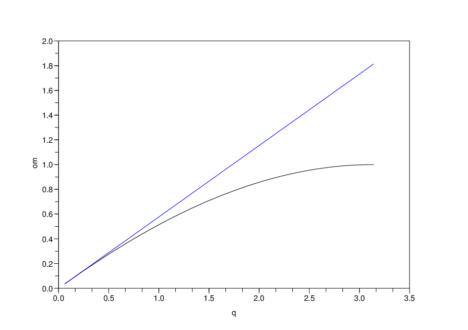
Consequently, the dispersion relation (41) behaves linearly in $q$ at fixed $A\neq 0$ when $q\rightarrow 0$ , and one has $\frac{\partial\omega}{\partial q}(0,0)=0$ , which corresponds to a vanishing “sound velocity” in the limit of small amplitudes. This property is consistent with the fact that, in the granular chain with a precompression $f_{0}$ , the sound velocity vanishes when $f_{0}\rightarrow 0$ . The graph of $\omega(.,A)$ is shown in figure 8 for $A=A_{0}={\|u_{0}\|}_{\infty}$ (so that $\omega(\pi,A_{0})=1$ ).

In what follows we formally analyze why the scaling (34) of ${\|u(.;q)\|}_{\infty}$ occurs when $q\rightarrow 0$ and heuristically compute the constant $k_{\alpha}$ present in the dispersion relation (42).

3.2. Long wave limit

Let us examine the limit $q\rightarrow 0$ more closely. We first normalize the solution of (11)-(12) computed in section 3.1 by setting $u=q^{\frac{2}{1-\alpha}}\,\tilde{u}$ , which yields

q^{2}\,\tilde{u}^{\prime\prime}(\xi)=V^{\prime}(\tilde{u}(\xi+q)-\tilde{u}(\xi))-V^{\prime}(\tilde{u}(\xi)-\tilde{u}(\xi-q)),

(43)

or equivalently

\tilde{u}^{\prime\prime}(\xi)=q^{\alpha-1}\,\frac{1}{q}\,\big(V^{\prime}[\,\frac{\tilde{u}(\xi+q)-\tilde{u}(\xi)}{q}\,]-V^{\prime}[\,\frac{\tilde{u}(\xi)-\tilde{u}(\xi-q)}{q}\,]\big),

(44)

where we have used the fact that $V^{\prime}(x)=-|x|^{\alpha}\,H(-x)$ . For $q\approx 0$ , we replace the right side of (44) by its continuum limit

\tilde{u}^{\prime\prime}(\xi)=q^{\alpha-1}\,\frac{d}{d\xi}\,V^{\prime}(\tilde{u}^{\prime}).

(45)

Setting $q=0$ in (45) and using the fact that $\tilde{u}(0)=0$ , we get the outer approximate solution

\tilde{u}_{o}(\xi)=\frac{\lambda}{\pi}\,\xi,\ \ \ \xi\in[0,\pi),

(46)

where $\lambda$ will be subsequently determined by a matching condition. When $q$ is small, equation (45) with $q=0$ does not describe the travelling wave profile in a boundary layer around $\xi=\pi$ where $\tilde{u}^{\prime}$ becomes large, and a rescaling of $\tilde{u}$ is necessary to capture the structure of the inner solution. Setting $s=q^{-1}\,(\xi-\pi)$ and $\tilde{u}(\xi)=y(s)$ , equation (43) becomes

y^{\prime\prime}(s)=V^{\prime}(y(s+1)-y(s))-V^{\prime}(y(s)-y(s-1)),\ \ \ s\in\mathbb{R}.

(47)

There exists an odd solution $y_{\rm{sol}}$ of (47) satisfying

\lim_{s\rightarrow-\infty}{y_{\rm{sol}}(s)}=k_{\alpha},\ \ \ \lim_{s\rightarrow+\infty}{y_{\rm{sol}}(s)}=-k_{\alpha},

(48)

where the convergence towards $k_{\alpha}$ is super-exponential and

k_{3/2}\approx 1.3567

(49)

(see appendix A). This solution corresponds to a solitary wave solution of (1) [38, 36, 15, 48] with velocity equal to unity. It yields the inner solution

\tilde{u}_{i}(\xi)=y_{\rm{sol}}(\frac{\xi-\pi}{q})

(50)

which agrees very well with the numerical solution in the vicinity of $\xi=\pi$ (see figure 9). Now let us match the outer and inner solutions at some point $\xi=\pi-q\,A(q)$ when $q\rightarrow 0$ , where $A(q)>0$ , $\lim_{q\rightarrow 0}{(q\,A(q))}=0$ and $\lim_{q\rightarrow 0}{A(q)}=+\infty$ . The matching condition reads

\lim_{q\rightarrow 0}{\lambda\,(1-\frac{q}{\pi}\,A(q))}=\lim_{q\rightarrow 0}{y_{\rm{sol}}(-A(q))},

which gives consequently $\lambda=k_{\alpha}$ . This approximation is in reasonable agreement with the numerical results since the value of $k_{3/2}$ deduced from figure 4 differs from the value (49) by $8.10^{-3}$ ( $q$ should be further decreased to get a better agreement). From the previous analysis, we deduce the following approximate solution of (43) obtained by summing the inner and outer solutions and substracting their common value at the matching point

\tilde{u}_{\rm{app}}(\xi)\approx\left\{\begin{array}[]{ll}{\displaystyle\frac{k_{\alpha}}{\pi}\,\xi+y_{\rm{sol}}(\frac{\xi-\pi}{q})-k_{\alpha},}&\xi\in[0,\pi],\\ {\displaystyle\frac{k_{\alpha}}{\pi}\,(\xi-2\pi)+y_{\rm{sol}}(\frac{\xi-\pi}{q})+k_{\alpha},}&\xi\in[\pi,2\pi].\end{array}\right.

(51)

The numerical and approximate solutions are compared in figure 10, which shows a good agreement between both profiles. The mathematical justification of this formal asymptotic analysis is left as an interesting open problem.

With approximation (51) at hand, let us now examine the wave structure in more details. Setting $a=q^{\frac{2}{\alpha-1}}$ , $\phi=\pi$ in (40) and using (51) yields approximate travelling wave solutions $x_{n}^{\rm{app}}(t)=\tilde{u}_{\rm{app}}(q(n-t)+\pi)$ with velocity equal to unity and $O(1)$ amplitude when $q\rightarrow 0$ . These solutions take the form

x_{n}^{\rm{app}}(t)=\frac{k_{\alpha}}{\pi}\,q(n-t)+y_{\rm{sol}}(n-t),\ \ \ \mbox{ for }|n-t|<\frac{\pi}{q}

(52)

and are $\frac{2\pi}{q}$ -periodic with respect to the moving frame coordinate $s=n-t$ . These waves consist of a succession of compression solitary waves, separated by large regions of free flight (of size $O(q^{-1})$ ) where particles move at a constant $O(q)$ velocity and equal gaps of size $O(q)$ are present between adjacent beads.

3.3. Compacton solutions

Several approximations of compression solitary waves with compact supports have been derived in the literature [37, 38, 4], in order to approximate exact solitary wave solutions of (1) decaying super-exponentially [15, 48]. However, the existence of exact solitary wave solutions of (1) with compact support remained an open question. Such solutions are supported by different classes of Hamiltonian PDE with fully-nonlinear dispersion, and have been known as compactons after the work of Rosenau and Hyman [41]. Nonlinear PDE supporting compactons can be introduced to analyze lattices with fully nonlinear interactions near a continuum limit. In this context, a common scenario is the transition from a compacton to a noncompact (super-exponentially localized) solution when passing from the continuum model to the discrete lattice [4] (see also [42, 29] for similar results in the context of discrete breather solutions).

In contrast to this situation, we show in this section that the numerical results of sections 3.1 imply the existence of compactons for the full lattice (1). This result is due to the occurence of free flight analyzed prevously, made possible by the unilateral character of Hertzian interactions, which vanish when beads are not in contact.

Let us consider the solutions $u(\xi;q)$ of (11)-(12) obtained numerically. These solutions behave linearly on the intervals $I_{0}=[-\ell(q),\ell(q)]$ and $I_{1}=[2\pi-\ell(q),2\pi+\ell(q)]$ . Denoting by $p(q)=u^{\prime}(0;q)$ their slope in these intervals, we have $u(\xi;q)=p(q)\,\xi$ on $I_{1}$ and $u(\xi;q)=p(q)\,(\xi-2\pi)$ on $I_{2}$ .

In what follows we assume $F(q)=2\ell(q)/q\geq 1$ , which corresponds to fixing $q\leq q_{k}\approx 1.8$ (see figure 7). This condition can be interpreted as follows. In the case of a strict inequality $F(q)>1$ , in a chain of beads where the wave $u(\xi;q)$ propagates, we have seen that two packets of interacting beads defined by (37) are always separated by some beads in free flight, hence $u(\xi;q)$ can be interpreted as a periodic train of independent pulses of finite width (i.e. compactons). Moreover, under the assumption $F(q)\geq 1$ , the length of the intervals $I_{1}$ and $I_{2}$ is larger than the delay $q$ involved in (11).

If $F(q)\geq 1$ , the solution $u(\xi;q)$ can be linearly extended in order to get a new solution of (11), defined by

U_{q}(\xi)=\left\{\begin{array}[]{ccc}p(q)\,\xi&\mbox{ for }&\xi\leq-\ell(q),\\ u(\xi;q)&\mbox{ for }&\xi\in[-\ell(q),2\pi+\ell(q)],\\ p(q)\,(\xi-2\pi)&\mbox{ for }&\xi\geq 2\pi+\ell(q).\end{array}\right.

(53)

The profile of $U_{q}$ is plotted in figure 11 for $q\approx 0.88$ . Let us check that $U_{q}$ defines a solution of (11) when $F(q)\geq 1$ (for notational simplicity we shall omit the $q$ -dependency). For $\xi\in I^{-}=(-\infty,\ell]$ we have $U^{\prime\prime}(\xi)=0$ , $U(\xi+q)-U(\xi)\geq 0$ and $U(\xi)-U(\xi-q)\geq 0$ , hence $U$ is a solution of (11) on $I^{-}$ . The same properties hold true for $\xi\in I^{+}=[2\pi-\ell,+\infty)$ . Moreover, $U$ is a solution of (11) for $\xi\in I^{c}=[q-\ell,2\pi+\ell-q]$ because $U=u$ and $\tau_{\pm q}U=\tau_{\pm q}u$ on $I^{c}$ . Since the condition $F\geq 1$ is equivalent to having $\mathbb{R}=I^{-}\cup I^{c}\cup I^{+}$ , $U$ defines a solution of (11) on $\mathbb{R}$ .

The solutions of (11) defined by (53) correspond to travelling wave solutions of (1) given by

X_{n}(t)=a\,U_{q}(q\,n-a^{\frac{\alpha-1}{2}}t+\phi),

(54)

where $a>0$ , $q\leq q_{k}$ and $\phi\in\mathbb{R}$ are parameters. Moreover, by Galilean invariance of (1), we deduce another family of solutions

\tilde{X}_{n}(t)=X_{n}(t)+v\,t

(55)

where we fix

v=a^{\frac{\alpha+1}{2}}\,p(q).

(56)

These solutions correspond to single compactons. Indeed, they consist of travelling waves, in the sense that bead velocities $\dot{X}_{n}(t)$ and relative displacements $X_{n}(t)-X_{n-1}(t)$ are functions of $n-c\,t$ with $c=q^{-1}a^{\frac{\alpha-1}{2}}$ . Moreover, each bead remains stationary except in a finite time interval where it experiences a compression. For a bead with index $n$ , compression occurs when $q\,n-a^{\frac{\alpha-1}{2}}t+\phi\in(\ell(q),2\pi-\ell(q))$ , i.e. when $U_{q}$ does not behave linearly. Fixing $\phi=-\ell(q)$ , the support of the moving compacton at time $t$ corresponds to $n\in(c\,t,c\,t+N(q))$ , where $N(q)$ is defined by (38).

Beads outside the support are separated by equal gaps of size $\Delta=a\,p(q)\,q$ and each bead position is shifted by $2\pi ap(q)$ after the passage of the compacton. The gap $\Delta$ depends on the parameters $a$ and $q$ , or equivalently on the compacton width $N(q)$ and velocity $c$ . Fixing $c=1$ and letting $q\rightarrow 0$ , the gap becomes $O(q)$ and the compacton profile converges towards the classical solitary wave in the compression region (see section 3.2).

Similarly to (53), one can obtain a family of $2$ -compacton solutions of (11) by gluing the solutions $U_{q}$ and $U_{q,\theta}^{(1)}(\xi)=p(q)\,\theta+U_{q}(\xi-2\pi-\theta)$ . Let us define

U^{(2)}_{q,\theta}(\xi)=\left\{\begin{array}[]{ccc}U_{q}(\xi)&\mbox{ for }&\xi\leq 2\pi+\theta+\ell(q),\\ U_{q,\theta}^{(1)}(\xi)&\mbox{ for }&\xi\geq 2\pi-\ell(q),\end{array}\right.

(57)

where $\theta=q\,d$ , $d\geq 0$ is a parameter and $q\in(0,q_{k}]$ , so that $q\leq 2\ell(q)$ . The graph of $U^{(2)}_{q,\theta}$ is illustrated by figure 11 (note that $U_{q}$ and $U_{q,\theta}^{(1)}$ coincide on $[2\pi-\ell(q),2\pi+\theta+\ell(q)]$ ). Let us check that $U^{(2)}_{q,\theta}$ defines a solution of (11) (for simplicity we shall omit dependency in $q$ and $\theta$ in notations). Firstly, $U^{(2)}$ is a solution of (11) for $\xi\in J^{-}=(-\infty,2\pi+\theta+\ell-q]$ because $U^{(2)}=U$ and $\tau_{\pm q}U^{(2)}=\tau_{\pm q}U$ on $J^{-}$ . Similarly, $U^{(2)}$ is a solution of (11) on $J^{+}=[2\pi-\ell+q,+\infty)$ because $U^{(2)}=U^{(1)}$ and $\tau_{\pm q}U^{(2)}=\tau_{\pm q}U^{(1)}$ on $J^{+}$ . If $q\leq\ell+\theta/2$ we have $J^{-}\cup J^{+}=\mathbb{R}$ and thus $U^{(2)}$ defines a solution of (11) on $\mathbb{R}$ . Moreover, if $\ell+\theta/2<q\leq 2\ell$ , then we have $(U^{(2)})^{\prime\prime}(\xi)=0$ , $U^{(2)}(\xi+q)-U^{(2)}(\xi)>0$ and $U^{(2)}(\xi)-U^{(2)}(\xi-q)>0$ for all $\xi\in J^{c}=(2\pi+\theta+\ell-q,2\pi-\ell+q)$ , hence $U^{(2)}$ is a solution of (11) on $J^{c}$ , which yields a solution of (11) on $\mathbb{R}=J^{-}\cup J^{c}\cup J^{+}$ .

Each solution of (1)

\tilde{X}_{n}(t)=a\,U^{(2)}_{q,\theta}(q\,n-a^{\frac{\alpha-1}{2}}t+\phi)+v\,t

(58)

with $v$ defined by (56) consists of two independent compactons separated by the distance $F(q)+d$ , with stationary beads outside the compactons. Similarly, generalizing the above construction would allow to define an infinity of solutions of (1), corresponding to an arbitrary number of independent compactons with variable compacton spacing.

Note that the remark made here on the existence of compactons follows from the numerical results obtained on problem (11)-(12) for wavenumbers $q\leq q_{k}$ . Obtaining an analytical proof of the existence of compactons remains an open problem.

3.4. Error minimization

In this section we evaluate and improve the numerical precision of the computations performed in section 3.1. Our numerical approach is in the same spirit as former computational methods developed to analyze the propagation of discrete breathers in nonlinear lattices [5] (see also [11]).

We consider a chain of $100$ particles with periodic boundary conditions

x_{n+N}(t)=x_{n}(t),\ \ \ N=100,

(59)

so that the lattice period is an integer multiple of the wavelength $\lambda=2\pi/q=100/m$ for our discrete set of values of $q$ . We fix $a={\|u(.;q)\|}_{\infty}^{-1}$ in (40), where $u(.;q)$ is the solution of (11)-(12) that was computed numerically for different values of $q$ . We use the resulting profile as an initial condition in system (1), which determines a periodic travelling wave solution $X_{n}=(x_{n},\dot{x}_{n})$ . Numerical integrations are performed using the standard ODE solver of the software package Scilab, where we have fixed the relative and absolute error tolerances to $10^{-12}$ and $10^{-14}$ respectively. For each solution $u(.;q)$ , we compute the relative residual error

E(q)=\frac{{\|{\{X_{n+1}(\mathcal{T})-X_{n}(0)\}}_{n}\|}_{\infty}}{{\|{\{X_{n}(0)\}}_{n}\|}_{\infty}}

with $\mathcal{T}=q\,a^{\frac{1-\alpha}{2}}$ , so that an exact travelling wave solution with velocity $\mathcal{T}^{-1}$ would cancel $E(q)$ . The inverse wave velocity $\mathcal{T}(q)$ is consequently given by

\mathcal{T}(q)=q\,{\|u(.;q)\|}_{\infty}^{\frac{\alpha-1}{2}}.

(60)

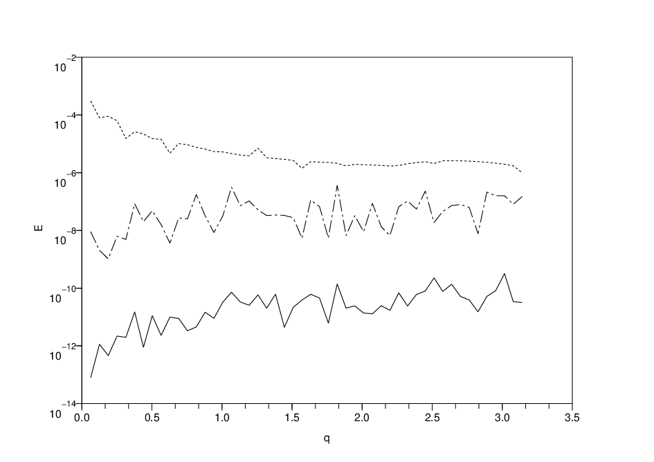
Figure 12 displays the graph of $E(q)$ (dotted line). With our numerical solution, this error remains less than $h^{2}\approx 10^{-5}$ for $q\geq 6\pi/25$ and grows when $q$ is further decreased, reaching $3.10^{-4}$ at $q=\pi/50$ . We attribute these larger errors to the sharpness of the travelling wave in the compression region when $q$ is sufficiently decreased. One way to improve the results would consist in discretizing (11)-(12) with a nonuniform mesh, thinner in the compression region. However, in what follows we use a different approach which decreases the residual error by several orders of magnitude on the whole range of wavenumbers $q$ .

We use the Gauss-Newton method [12] in order to determine a refined initial condition ${\{X_{n}(0)\}}_{n=1,\ldots,N}$ minimizing ${\|{\{X_{n+1}(\mathcal{T})-X_{n}(0)\}}_{n}\|}_{2}^{2}$ (the Newton method is not directly applicable due to the noninvertibility of the Jacobian matrix at the exact solution). The improved initial condition obtained in this way for a given wavenumber $q$ will be denoted by $X_{n}(0)=X_{n}^{(q)}$ . To compute these solutions, we initialize the Gauss-Newton iteration using the numerical solutions $u(.;q)$ of (11)-(12) obtained previously, since they already provide initial conditions quite close to the optima. To reduce the computational cost, we modify the Gauss-Newton method by actualizing the Jacobian matrix only at some steps of the iteration, when a re-evaluation is required to decrease the residual error. The residual error $E(q)$ obtained with this numerical method drops to $3.10^{-10}$ or less, as shown in figure 12 (full line). At the end of the Gauss-Newton iteration ( $k$ th iteration), the relative difference between the last two iterates $r(q)=\frac{{\|{\{X_{n}^{(k)}(0)-X_{n}^{(k-1)}(0)\}}_{n}\|}_{\infty}}{{\|{\{X_{n}^{(k)}(0)\}}_{n}\|}_{\infty}}$ drops below $4.10^{-7}$ (see figure 12, dash-dot line).

Above a critical value $q_{c}\approx 0.9$ , the initial conditions computed as indicated above yield travelling waves that remain practically unchanged over very long times when propagating along the lattice (see figure 13 for an example). The situation changes drastically below $q_{c}$ because the travelling waves become unstable, yielding an amplification at exponential rate of the initially small errors made on the initial condition. This situation is described in figure 14 for $q=7\pi/25$ . The travelling wave is destroyed by a instability at $t\approx 360\approx 303\,\mathcal{T}$ , which rapidly drives the system into a disordered regime. These instabilities will be described in more detail in the next section.

3.5. Wave instabilities

In this section we consider the dynamical equation (1) of the granular chain with $N=100$ particles and periodic boundary conditions, and numerically study the stability of the travelling wave solutions of section 3.4. We recall that these travelling waves take the form (40), where $u(.;q)$ is the solution of (11)-(12) computed numerically for a given value of $q$ , and where we fix $a={\|u(.;q)\|}_{\infty}^{-1}$ to renormalize the solution. We rewrite equation (1) in the compact form $\dot{X}=f(X)$ with $X(t)=(X_{1}(t),\ldots,X_{N}(t))^{t}\in\mathbb{R}^{2N}$ and $X_{n}=(x_{n},\dot{x}_{n})$ , and denote by $X^{(q)}(t)$ the solutions corresponding to travelling waves.

Since the solution $X^{(q)}(t)$ is time-periodic with period $\tau(q)=2\pi a^{\frac{1-\alpha}{2}}$ , its stability can be analyzed using Floquet theory. Let us denote by $\mathcal{R}(t;t_{0})$ the resolvent matrix of the linearized equation $\dot{X}=Df(X^{(q)}(t))\,X$ and $\Phi_{q}=\mathcal{R}(\tau(q);0)$ the associated monodromy matrix. The solution $X^{(q)}(t)$ is called spectrally stable if all eigenvalues of ${\Phi}_{q}$ lie on the unit circle, and $X^{(q)}(t)$ is unstable if there exists an eigenvalue of modulus strictly larger than $1$ (see e.g. [10, 1]). In other words, the spectral radius $\rho(\Phi_{q})$ determines if $X^{(q)}(t)$ is unstable ( $\rho(\Phi_{q})>1$ ) or spectrally stable ( $\rho(\Phi_{q})=1$ ).

Since $X^{(q)}(t)$ is a periodic travelling wave and periodic boundary conditions are used, one can equivalently determine wave stability using a monodromy matrix modulo shifts. This approach reduces the length of numerical integration significantly at low wavenumbers, since the linearized equations are integrated over an interval of length $\mathcal{T}(q)=\frac{q}{2\pi}\tau(q)$ . Moreover, it describes more conveniently the growth of perturbations in a frame moving with the waves in the linear approximation.

To be more precise, let us denote by $\mathcal{S}$ the spatial shift $\mathcal{S}\,X=(X_{2},\ldots,X_{N},X_{1})^{t}$ associated to periodic boundary conditions. The initial condition $X^{(q)}(0)$ corresponding to a travelling wave solution is a fixed point of the map $\mathcal{N}_{q}$ defined by

\mathcal{N}_{q}(X(0))=\mathcal{S}\,X(\mathcal{T}(q)),

where the inverse wave velocity $\mathcal{T}(q)$ is given by (60). Let us introduce the monodromy matrix modulo shift $\mathcal{F}_{q}=D\mathcal{N}_{q}(X^{(q)}(0))$ , which takes the form

\mathcal{F}_{q}=\mathcal{S}\,\mathcal{R}(\mathcal{T}(q);0).

Recalling that $q=2m\pi/N$ ( $1\leq m\leq N/2$ ), we have $\tau(q)=\frac{N}{m}\,\mathcal{T}(q)$ . Thanks to the invariance $\mathcal{S}\,X^{(q)}(t+\mathcal{T}(q))=X^{(q)}(t)$ , one has $\mathcal{S}\,\mathcal{R}(t+\mathcal{T};t_{0})=\mathcal{R}(t;t_{0}-\mathcal{T})\,\mathcal{S}$ , which implies

\mathcal{F}_{q}^{N}=\Phi_{q}^{m}.

Consequently one has $\rho(\Phi_{q})={\rho(\mathcal{F}_{q})}^{N/m}$ , i.e. $X^{(q)}(t)$ is unstable for $\rho(\mathcal{F}_{q})>1$ and spectrally stable if $\rho(\mathcal{F}_{q})=1$ .

The spectral radius of $\mathcal{F}_{q}$ is plotted in figure 15 as a function of $q$ (these results are obtained using the software package Scilab, for which matrix eigenvalue computations are based on the Lapack routine DGEEV). These results show that the travelling waves are unstable below the critical value $q_{c}\approx 0.9$ . The growth rate of the instability in the linear approximation is maximal for $q=q_{m}\approx 0.56$ , and decreases rapidly when $q\rightarrow 0$ and $q\rightarrow q_{c}$ . Figure 16 shows the evolution of the eigenvalues of $\mathcal{F}_{q}$ when $q$ is varied in this parameter region. One can see that the number of unstable modes rapidly increases below $q=q_{c}$ .

According to figure 6 we have $N(q_{c})\approx 3$ , i.e. instabilities show up when the average number $N(q)$ of adjacent interacting beads becomes $\geq 3$ . This case corresponds to the maximal number of adjacent interacting beads becoming $\geq 4$ . This phenomenon can be intuitively understood through the results of [47], where the travelling wave stability was numerically established for a three-ball chain (with fixed center of mass) using Poincaré sections. However, as it follows from our numerical results, the interactions of the three-ball packets with additional beads generate instabilities as soon as $q<q_{c}$ .

The weakness of the linear instability for $q\approx 0$ is consistent with the convergence of the travelling waves towards the classical Hertzian solitary wave (section 3.2), given the fact that the Hertzian solitary wave appears structurally robust in dynamical simulations.

Now let us describe how these instabilities act on the wave profiles. When $q$ is slightly below $q_{c}$ , the early stage of the instability generates two large regions of average compression separated by two large regions of average extension (see figure 17). This transitory state disappears rapidly and a disordered regime settles, as shown previously in figure 14. When $q$ reaches $q_{m}$ , the large-scale transitory state is not visible any more and the system directly evolves from the regular travelling wave towards the disordered regime. The instability of the travelling waves is observed up to the long wave limit, where it manifests differently from the instability at $q\approx q_{c}$ . A slow dispersion of the compression pulse occurs (see figure 18, top right plot), and subsequent collisions of dispersive waves with the shock generate a fast instability. A closer view of the transition from dispersive travelling waves to spatiotemporal disorder is provided by the lower plot of figure 18. In these different examples, we interpret the abrupt transition to a disordered regime as the result of the large number of unstable modes.

It is interesting to note that the disordered regime that occurs after these instabilities coexists with some partial order, because transitory large-scale organized structures appear intermittently. This phenomenon is illustrated by figure 19 (lower plots). These structures seem to result from the interactions of travelling waves that coexist with the disordered dynamics. This is shown in the upper plot of figure 19, which provides the spatiotemporal evolution of bead displacements in grey levels. The region corresponding to $t\in[0,140]$ (nearly uniform at the scale of the figure) corresponds to the propagation of an almost unperturbed periodic travelling wave with wavenumber $q=9\pi/50\approx q_{m}$ , and spatiotemporal disorder occurs for $t\geq 140$ after an instability. In this region, the presence of stripes reveals counter-propagating travelling waves.

Above the critical value $q_{c}\approx 0.9$ , we have observed very slow modulational instabilities by integrating (1), starting from small random perturbations of travelling waves with specific wavenumbers. However, the above Floquet analysis is not sufficiently precise to correctly account for these very small instabilities in the linear regime, because they may be overhelmed by numerical errors.

4. Discussion

Even though the Hertzian granular chain is commonly denoted as a “sonic vacuum”, we have shown that long granular chains sustain periodic travelling waves on a full range of wavenumbers. We have proved the existence of a family of periodic travelling waves with wavenumbers $q$ close to $\pi$ and profiles close to binary oscillations. Using numerical continuation in $q$ , we have been able to follow this branch of solutions up to the long wave limit $q\approx 0$ , where they become close to a solitary wave inside small compression regions.

The waves we have obtained display unusual properties, due to the fully nonlinear and unilateral character of Hertzian interactions. Each bead periodically undergoes a compression phase followed by a free flight, a transition associated with a limited smoothness of the wave profile (i.e. the corresponding solutions of (16) are $C^{3}$ but not $C^{4}$ at the onset of free flight). Moreover, below a critical value $q=q_{k}\approx 1.8$ , the waves can be considered as a periodic train of independent compactons separated by beads in free flight. These numerical findings imply the existence of an isolated compacton in granular chains, when beads are separated by equal gaps outside the compression wave, the gaps depending on the velocity and width of the compacton.

An interesting open problem is to prove analytically the existence of the periodic travelling waves obtained numerically, far from the limit of binary oscillations. For $q\approx 0$ , this problem is equivalent to the existence of a family of compactons close to the Hertzian solitary wave, in the limit when the gaps between beads become small.

From a dynamical point of view, below a critical wavenumber $q_{c}\approx 0.9$ , we have observed fast instabilities of the periodic travelling waves leading to a disordered regime. This threshold was attained when the average number of adjacent interacting beads becomes $\geq 3$ , or equivalently when the maximal number of adjacent interacting beads becomes $\geq 4$ . The travelling waves appeared far more robust for $q>q_{c}$ , i.e. when the number of adjacent interacting beads was always $\leq 3$ . This can be intuitively understood through the results of [47], where the travelling wave stability was numerically established for a three-ball chain with fixed center of mass. However, as soon as $q<q_{c}$ , we have shown numerically that the interactions of the three-ball packets with additional beads generate instabilities. These instabilities persist up to $q\approx 0$ , where they display a slower growth rate in the linear approximation.

As illustrated by figure 18, a cumulative instability effect is present due to periodic boundary conditions, since all perturbations left behind the compression pulse interact subsequently with it. If the existence of isolated compactons can be mathematically established, it would be interesting to analyze their spectral stability and determine if the above exponential instabilities persist. More generally, the spectral stability analysis of periodic travelling waves would deserve more investigations. Above the critical value $q_{c}\approx 0.9$ , it would be interesting to determine for which wavenumbers the waves are stable or slowly unstable. This question requires more refined numerical methods to resolve very slow instabilities present in this parameter regime. In addition, unusual perturbations of Floquet eigenvalues may arise from the limited smoothness of Hertzian interactions.

Another question concerns the generation of stable periodic travelling waves in driven granular chains, in relation with possible experimental realizations. In principle, the travelling waves we have analyzed could be generated in finite systems, provided the motions of the first and last beads are imposed (following an exact travelling wave profile) and starting from an exact initial condition. However these conditions are extremely restrictive. In addition, dissipative effects should be also considered for practical applications. In this context, it would be interesting to study how to generate periodic travelling waves from simpler initial conditions and driving signals in dissipative granular systems.

Appendix A Compression solitary waves

In this appendix we recall some classical properties of solitary waves in granular chains which are used in section 3.2 for the analysis of the long wave regime.

Consider travelling wave solutions of (1) taking the form $x_{n}(t)=y(s)$ , where $s=n-c\,t$ . The function $y$ satisfies

c^{2}\,y^{\prime\prime}(s)=V^{\prime}(y(s+1)-y(s))-V^{\prime}(y(s)-y(s-1)),\ \ \ s\in\mathbb{R},

(61)

where we recall that $V^{\prime}(x)=-|x|^{\alpha}\,H(-x)$ , $\alpha>1$ and $H$ denotes the Heaviside function. Up to rescaling $y$ , one can fix $c=\pm 1$ in (61) without loss of generality. In that case, the renormalized relative displacements $r(s)=y(s+\frac{1}{2})-y(s-\frac{1}{2})$ satisfy

r^{\prime\prime}(s)=V^{\prime}(r(s+1))-2V^{\prime}(r(s))+V^{\prime}(r(s-1)),\ \ \ s\in\mathbb{R}.

(62)

There exists a negative solution of (62) satisfying $\lim\limits_{s\rightarrow\pm\infty}{r(s)}=0$ and $r^{\prime}(0)=0$ , which is known to decay super-exponentially [21, 36, 30, 15, 48]. This solution corresponds to an exact solitary wave solution of (1) close to Nesterenko’s approximate solution, with velocity equal to unity. Figure 20 shows the solitary wave profile computed numerically, using the same numerical scheme as for periodic waves (except we change the boundary conditions and use an explicit approximation of $r$ derived by Ahnert and Pikovsky [4] to initialize the Broyden method). Our results agree with the ones of references [4, 15, 48], in particular the solution we obtain is even in $s$ .

To recover $y$ from $r$ , we note that the Poisson equation

-y^{\prime\prime}(s)=f(s),\ \ \ s\in\mathbb{R},

admits for all odd functions $f$ decaying exponentially at infinity a unique odd and bounded solution given by $y(s)=\int_{\mathbb{R}}{G(s,t)\,f(t)\,dt}$ , where

G(s,t)=\frac{1}{2}\,H(st)\,(|t+s|-|t-s|).

Moreover, one has

\lim_{s\rightarrow\pm\infty}{y(s)}=\pm\int_{0}^{+\infty}{t\,f(t)\,dt},

(63)

the convergence being exponential. Equation (61) with $c=1$ can be rewritten

y^{\prime\prime}(s)=V^{\prime}(r(s+\frac{1}{2}))-V^{\prime}(r(s-\frac{1}{2})),

where the right side is odd in $s$ due to the evenness of $r$ . Consequently, we obtain a solution of (61) with $c=1$ , given by

y(s)=\int_{\mathbb{R}}{G(s,t)\,[V^{\prime}(r(t-\frac{1}{2}))-V^{\prime}(r(t+\frac{1}{2}))]\,dt},

(64)

and satisfying

\lim_{s\rightarrow-\infty}{y(s)}=k_{\alpha},\ \ \ \lim_{s\rightarrow+\infty}{y(s)}=-k_{\alpha},

(65)

where we have

k_{\alpha}=-\int_{0}^{+\infty}{V^{\prime}(r(s))\,ds}

(66)

by virtue of (63) (this simplification is obtained using the evenness of $r$ and elementary changes of variables in the integral). Note that a simpler formula can be derived for the numerical computation of $y$ , using the fact that

y(s)=y(s-N-1)+\sum_{k=0}^{N}{r(s-k-\frac{1}{2})}.

Letting $N\rightarrow+\infty$ and using the evenness of $r$ yields

y(s)=k_{\alpha}+\sum_{k=0}^{+\infty}{r(k+\frac{1}{2}-s)}.

Then setting $s=0$ gives

k_{\alpha}=-\sum_{k=0}^{+\infty}{r(k+\frac{1}{2})},

(67)

and consequently

y(s)=\sum_{k=0}^{+\infty}{r(k+\frac{1}{2}-s)-r(k+\frac{1}{2})}.

(68)

Using formula (67) we numerically obtain $k_{3/2}\approx 1.3567$ .

Acknowledgements: The author is grateful to anonymous referees for several suggestions which essentially improved the paper, in particular for pointing out the question of the existence of compactons. Helpful discussions with J. Malick, B. Brogliato, A.R. Champneys and P.G. Kevrekidis are also acknowledged.

References

[1] R. Abraham and J.E. Marsden, Foundations of Mechanics, Second Edition, Addison-Wesley Publishing Company (1987).
[2] M. Abramowitz and I.A. Stegun, eds. Handbook of Mathematical Functions, National Bureau of Standards, 1964 (10th corrected printing, 1970), www.nr.com.
[3] V. Acary and B. Brogliato. Concurrent multiple impacts modelling: Case study of a 3-ball chain, Proc. of the MIT Conference on Computational Fluid and Solid Mechanics, 2003 (K.J. Bathe, Ed.), Elsevier Science, 1836-1841.
[4] K. Ahnert and A. Pikovsky. Compactons and chaos in strongly nonlinear lattices, Phys. Rev. E 79 (2009), 026209.
[5] S. Aubry and T. Cretegny. Mobility and reactivity of discrete breathers, Physica D 119 (1998), 34-46.
[6] N. Boechler, G. Theocharis, S. Job, P.G. Kevrekidis, M.A. Porter and C. Daraio. Discrete breathers in one-dimensional diatomic granular crystals, Phys. Rev. Lett. 104 (2010), 244302.
[7] D.K. Campbell et al, editors. The Fermi-Pasta-Ulam problem : the first $50$ years, Chaos 15 (2005).
[8] R. Carretero-González, D. Khatri, M.A. Porter, P.G. Kevrekidis and C. Daraio. Dissipative solitary waves in granular crystals, Phys. Rev. Lett. 102 (2009), 024102.
[9] A. Chatterjee. Asymptotic solutions for solitary waves in a chain of elastic spheres, Phys. Rev. E 59 (1999), 5912-5918.
[10] C. Chicone, Ordinary differential equations with applications, Texts in applied mathematics 34, Springer (1999).
[11] T. Cretegny and S. Aubry. Spatially inhomogeneous time-periodic propagating waves in anharmonic systems, Phys. Rev. B 55 (1997), R11929-R11932.
[12] J.E. Dennis, Jr. and R.B. Schnabel, Numerical methods for unconstrained optimization and nonlinear equations, SIAM Classics in Applied Mathematics 16, SIAM (Society for Industrial and Applied Mathematics), 1996.
[13] W. Dreyer, M. Herrmann and A. Mielke. Micro-macro transition in the atomic chain via Whitham’s modulation equation, Nonlinearity 19 (2006), 471-500.
[14] W. Dreyer and M. Herrmann. Numerical experiments on the modulation theory for the nonlinear atomic chain, Physica D 237 (2008), 255-282.
[15] J.M. English and R.L. Pego. On the solitary wave pulse in a chain of beads, Proc. Amer. Math. Soc. 133, n. 6 (2005), 1763-1768.
[16] E. Falcon. Comportements dynamiques associés au contact de Hertz : processus collectifs de collision et propagation d’ondes solitaires dans les milieux granulaires, PhD thesis, Université Claude Bernard Lyon 1 (1997).
[17] A.M. Filip and S. Venakides. Existence and modulation of traveling waves in particle chains, Comm. Pure Appl. Math. 52 (1999), 693-735.
[18] F. Fraternali, M. A. Porter, and C. Daraio. Optimal design of composite granular protectors, Mech. Adv. Mat. Struct. 17 (2010), 1-19.
[19] G. Friesecke and R.L. Pego. Solitary waves on FPU lattices : I. Qualitative properties, renormalization and continuum limit, Nonlinearity 12 (1999), 1601-1627.
[20] G. Friesecke and R.L. Pego. Solitary waves on FPU lattices : IV. Proof of stability at low energy, Nonlinearity 17 (2004), 229-251.
[21] G. Friesecke and J.A Wattis. Existence theorem for solitary waves on lattices, Commun. Math. Phys. 161 (1994), 391-418.
[22] G. Fu. An extension of Hertz’s theory in contact mechanics, J. Appl. Mech. 74 (2007), 373-375.
[23] G. Gallavotti, editor. The Fermi-Pasta-Ulam Problem. A Status Report, Lecture Notes in Physics 728 (2008), Springer.
[24] M. Herrmann. Unimodal wave trains and solitons in convex FPU chains, Proc. Roy. Soc. Edinburgh A 140 (2010), 753-785.
[25] E. J. Hinch and S. Saint-Jean. The fragmentation of a line of ball by an impact, Proc. R. Soc. London, Ser. A 455 (1999), 3201-3220.
[26] A. Hoffman and C.E. Wayne. A simple proof of the stability of solitary waves in the Fermi-Pasta-Ulam model near the KdV limit (2008), arXiv:0811.2406v1 [nlin.PS].
[27] G. Iooss. Travelling waves in the Fermi-Pasta-Ulam lattice, Nonlinearity 13 (2000), 849-866.
[28] G. James. Nonlinear waves in Newton’s cradle and the discrete $p$ -Schrödinger equation (2010), arXiv:1008.1153v1 [nlin.PS]. To appear in Math. Mod. Meth. Appl. Sci., DOI No: 10.1142/S0218202511005763.
[29] G. James, P.G. Kevrekidis and J. Cuevas. Breathers in oscillator chains with Hertzian interactions (2011), arXiv:1111.1857v1 [nlin.PS].
[30] J.-Y. Ji and J. Hong. Existence criterion of solitary waves in a chain of grains, Phys. Lett. A 260 (1999), 60-61.
[31] K.L. Johnson. Contact mechanics, Cambridge Univ. Press, 1985.
[32] P.A. Johnson and X. Jia. Nonlinear dynamics, granular media and dynamic earthquake triggering, Nature 437 (2005), 871-874.
[33] C. Liu, Z. Zhao and B. Brogliato. Frictionless multiple impacts in multibody systems. I. Theoretical framework. Proc. R. Soc. A-Math. Phys. Eng. Sci., 464 (2008), 3193-3211.
[34] C. Liu, Z. Zhao and B. Brogliato. Frictionless multiple impacts in multibody systems. II. Numerical algorithm and simulation results, Proc. R. Soc. A-Math. Phys. Eng. Sci., 465 (2009), 1-23.
[35] W. Ma, C. Liu, B. Chen and L. Huang. Theoretical model for the pulse dynamics in a long granular chain, Phys. Rev. E 74 (2006), 046602.
[36] R.S. MacKay. Solitary waves in a chain of beads under Hertz contact, Phys. Lett. A 251 (1999), 191-192.
[37] V.F. Nesterenko. Propagation of nonlinear compression pulses in granular media, J. Appl. Mech. Tech. Phys. 24 (1983), 733-743.
[38] V.F. Nesterenko, Dynamics of heterogeneous materials, Springer Verlag, 2001.
[39] A. Pankov. Travelling waves and periodic oscillations in Fermi-Pasta-Ulam lattices, Imperial College Press, London, 2005.
[40] M. Porter, C. Daraio, I. Szelengowicz, E.B. Herbold and P.G. Kevrekidis. Highly nonlinear solitary waves in heterogeneous periodic granular media, Physica D 238 (2009), 666-676.
[41] P. Rosenau and J.M. Hyman. Compactons: solitons with finite wavelength, Phys. Rev. Lett. 70 (1993), 564.
[42] P. Rosenau and S. Schochet. Compact and almost compact breathers: a bridge between an anharmonic lattice and its continuum limit, Chaos 15 (2005), 015111.
[43] J. Schmittbuhl, J.-P. Vilotte and S. Roux. Propagative macrodislocation modes in an earthquake fault model, Europhys. Lett. 21 (1993), 375-380.
[44] S. Sen, J. Hong, J. Bang, E. Avalos and R. Doney. Solitary waves in the granular chain, Physics Reports 462 (2008), 21-66.
[45] S. Sen, M. Manciu and J.D. Wright. Soliton-like pulses in perturbed and driven Hertzian chains and their possible applications in detecting buried impurities, Phys. Rev. E 57 (1998), 2386-2397.
[46] J.-A. Sepulchre and R.S. MacKay. Localized oscillations in conservative or dissipative networks of weakly coupled autonomous oscillators, Nonlinearity 10 (1997), 679-713 .
[47] Y. Starosvetsky and A.F. Vakakis. Traveling waves and localized modes in one-dimensional homogeneous granular chains with no precompression, Phys. Rev. E 82 (2010), 026603.
[48] A. Stefanov and P.G. Kevrekidis. On the existence of solitary traveling waves for generalized Hertzian chains, J. Nonlinear Sci. (2012), DOI: 10.1007/s00332-011-9119-9.