跳到论文正文
W Papers独立论文阅读器 arXiv:1203.0559 论文正文 计算阅读时间 · 0%
引用这篇论文根据当前论文元数据生成,正式投稿前建议核对。


License: arXiv.org perpetual non-exclusive license
arXiv:1203.0559v2 [hep-th] 21 May 2012

KUNS-2387

Large-NN reduction for 𝒩=2{\cal N}=2 quiver Chern-Simons theories on S3S^{3}

and localization in matrix models

Yuhma Asano** * e-mail address : yuhma@gauge.scphys.kyoto-u.ac.jp , Goro Ishiki†† † e-mail address : ishiki@post.kek.jp, Takashi Okada‡‡ ‡ e-mail address : okada@gauge.scphys.kyoto-u.ac.jp and Shinji Shimasaki§§ § e-mail address : shinji@gauge.scphys.kyoto-u.ac.jp

Department of Physics, Kyoto University
Kyoto, 606-8502, Japan

We study reduced matrix models obtained by the dimensional reduction of 𝒩=2{\cal N}=2 quiver Chern-Simons theories on S3S^{3} to zero dimension and show that if a reduced model is expanded around a particular multiple fuzzy sphere background, it becomes equivalent to the original theory on S3S^{3} in the large-NN limit. This is regarded as a novel large-NN reduction on a curved space S3S^{3}. We perform the localization method to the reduced model and compute the free energy and the vacuum expectation value of a BPS Wilson loop operator. In the large-NN limit, we find an exact agreement between these results and those in the original theory on S3S^{3}.

1 Introduction

The localization technique has attracted much attention in recent years as an efficient method of computing a class of physical quantities of our interest. For instance, it enables us to compute exactly BPS Wilson loops or partition functions in 4d 𝒩=2{\cal N}=2 supersymmetric Yang-Mills (SYM) theories [1] or those in 3d 𝒩=2{\cal N}=2 Chern-Simons (CS) theories coupled to some matter fields [2, 3, 4, 5, 6, 7]. In particular, predictions from their gravity duals, such as the N3/2N^{3/2} law of the free energy [8] in the ABJM theory[9], can be verified explicitly based on the localization method [3] and thus a remarkable progress has been made in testing the gauge/gravity correspondence [10].

In this paper, we use the localization method for another purpose. We apply it to a dimensionally reduced matrix model of a general 𝒩=2{\cal N}=2 non-chiral11 1 In quiver diagram, non-chiral means that for every arrow from node A to node B there is a corresponding arrow from node B to node A. quiver CS theory on S3S^{3} and show that there exists an equivalence in a large-NN limit between the reduced model and the original theory on S3S^{3}. This kind of large-NN equivalence on S3S^{3} was first discovered in [11] for 𝒩=4{\cal N}=4 SYM on R×S3R\times S^{3} (see also [14, 13, 12] for earlier discussions) and it is regarded as a novel type of the large-NN reduction extended to the case of S3S^{3}.

The original large-NN reduction initiated by Eguchi and Kawai asserts that a gauge theory on flat space-time in the planar limit is equivalent to a matrix model that is obtained by its dimensional reduction to lower dimensions [15]. This equivalence is significant not only because it realizes the emergence of space-time in matrix models, which is relevant in the context of the matrix model formulation for string theories [16], but also because this equivalence implies that the matrix models provide a non-perturbative formulation of planar gauge theories which is alternative to the lattice formulation. One may expect that supersymmetric theories can be described in terms of matrix models non-perturbatively based on this equivalence while it is generally difficult in the lattice formulation22 2 There are considerable recent developments in the lattice theories for supersymmetric theories [17]..

It is however well-known that this equivalence fails to hold due to the spontaneous U​(1)DU(1)^{D} symmetry breaking in the original Eguchi-Kawai model [18]. To overcome this difficulty, the quenching and the twisting prescriptions were proposed [18, 19, 20, 21, 22]. Although the symmetry breaking can be avoided by introducing such prescriptions at least when the theory has a sufficient number of fermions33 3 See [23, 24] for detail. , they do not preserve supersymmetry. Because of this, it had been difficult until recently to construct a non-perturbative formulation of supersymmetric gauge theories based on the large-NN reduction which keeps supersymmetry manifestly.

The novel large-NN reduction was proposed for theories on S3S^{3} [11]. It states that a reduced model, which is obtained by the dimensional reduction of a gauge theory on S3S^{3} to a point, becomes equivalent to the original gauge theory in the large-NN limit if the reduced model is expanded around a certain multiple fuzzy sphere background and a continuum limit is taken. In this proposal, the above-mentioned difficulty is avoided thanks to the curvature of S3S^{3}. On S3S^{3}, a gauge theory acquires a mass gap, which is inversely proportional to the radius of S3S^{3}, and hence does not possess a flat direction, which would lead the symmetry breaking and spoil the large-NN equivalence. This implies that the prescriptions are not needed in this case, so that a reduced model obtained from a supersymmetric gauge theory still keeps part of the original supersymmetry. One can therefore use the reduced model as a non-perturbative formulation of the supersymmetric theory on S3S^{3}. So far, such formulation has been considered for 𝒩=4{\cal N}=4 SYM [11], SYM with lower supersymmetry [25] and supersymmetric quiver CS theories [26]. The large-NN reduction has also been extended to the cases for more general manifolds such as group manifolds [27] and coset spaces [28].

In particular, the large-NN reduction for 𝒩=4{\cal N}=4 SYM on R×S3R\times S^{3} has been studied actively [29, 30, 31, 32] since it is relevant to testing the original version of the AdS/CFT correspondence for the type IIB string theory on A​d​S5×S5AdS_{5}\times S^{5}. The reduced model of 𝒩=4{\cal N}=4 SYM on R×S3R\times S^{3} is given by the plane wave matrix model (PWMM) [33, 34]. This model preserves S​U​(2|4)SU(2|4) symmetry, which can not be realized in the lattice formulation at present, so that it is expected to describe the original theory on S3S^{3} in the continuum limit without any fine-tuning. Based on this formulation, one can analyze numerically the strongly coupled regime of the planar 𝒩=4{\cal N}=4 SYM, which is mapped to the regime in the string theory where the supergravity or the semiclassical approximation is valid. The methods of the Monte Carlo simulation for matrix models proposed in [35, 36, 37] are available for the numerical computation. Thus, it gives a feasible way of testing the AdS/CFT correspondence44 4 See [38, 39] for preliminary results of such attempts..

Although the validity of such non-perturbative formulation of supersymmetric theories has been checked by some perturbative calculations [29, 30, 31, 32], it should be checked also for the strong coupling region. In this paper, we consider the large-NN reduction for 𝒩=2{\cal N}=2 non-chiral quiver CS theories on S3S^{3}. Applying the localization method, we compute the partition function and the one-point function of the great circular BPS Wilson loop operator in the reduced model. Then we prove the large-NN equivalence for these quantities to all orders in the perturbation theory. We also find that a saddle point configuration of the reduced matrix model is given as infinitely many copies of that in the original theory up to a cutoff effect, which is negligible in the continuum limit. This fact ensures that the equivalence also holds even in the strongly coupled regime.

So far, a similar test of the large-NN reduction has been done for the pure CS theory on S3S^{3} [40, 41]55 5 See also [42, 43]., which is a solvable topological field theory [44]. Since the path integral of the reduced model is easily performed in this case, it is possible to see the agreement of two theories through a direct calculation. Although the theory we consider in this paper contains dynamical degrees of freedom and hence is not so simple, the localization method enables us to verify the large-NN equivalence explicitly.

This paper is organized as follows. In section 2, we review known results on the computation of the partition function and the BPS Wilson loop operator in a general 𝒩=2{\cal N}=2 quiver CS theory. In section 3, we introduce the reduced model of the theory on S3S^{3} focusing on the supersymmetry transformation. We also perform the path integral of the reduced model by means of the localization. In section 4, we show the large-NN equivalence. We first extract a theory around the multiple fuzzy sphere background which creates S3S^{3} from the result of the localization and see that the theory reduces to a certain eigenvalue integral. By studying this integral, we see the equivalence both in the perturbation theory and in the saddle point equation. Section 5 is devoted to conclusion. In appendices, some details are gathered.

2 Localization in 𝒩=2{\cal N}=2 quiver CS theory on S3S^{3}

In this section, we review some known results for the localization in a 𝒩=2{\cal N}=2 quiver CS theory on S3S^{3} [2, 3, 4, 5]. We assume that the gauge group is given by a product of unitary groups, ⨂aU⁡(Na)\bigotimes_{a}U(N_{a}), and consider a general matter content. We set the radius of S3S^{3} to be one in this paper and our convention for the theory on S3S^{3} is summarized in appendix A.

In this theory, there are nilpotent supersymmetries, which we will call QQ symbolically in the following. The partition function is invariant under adding QQ-exact terms to the action. Hence the path integral can be localized onto the saddle points of the QQ-exact terms. For a gauge multiplet, the role of the QQ-exact term is played by the Yang-Mills (YM) action on S3S^{3} and for a matter multiplet by a part of the matter action. The saddle point configuration is given by the flat connection for the gauge field, which is trivial on S3S^{3}, namely, Aμ=0A_{\mu}=0 up to gauge transformation. Also all the matter fields are zero at the saddle point. The other bosonic fields in the vector multiplet, σ\sigma and DD, take nontrivial values at the saddle point. They are given by,

σ=−D=constant.\displaystyle\sigma=-D={\rm constant}. (2.1)

Then, the calculation of the partition function amounts to computing the 1-loop determinant at each saddle point. The result is written as a summation over contributions from all the saddle points, namely in our case, as an integral over the constant matrix σ\sigma for each gauge multiplet. In the following, we will work in the gauge in which σ\sigma’s in all the gauge multiplets are diagonalized, so that the integration measure has the Vandermonde determinant as ∫∏id​σi​∏i<j(σi−σj)2\int\prod_{i}d\sigma_{i}\prod_{i<j}(\sigma_{i}-\sigma_{j})^{2} for each gauge multiplet.

The contribution from a vector multiplet is given by

∏i<j(sinh⁡(π⁡(σi−σj))π⁡(σi−σj))2,\displaystyle\prod_{i<j}\left(\frac{\sinh(\pi(\sigma_{i}-\sigma_{j}))}{\pi(\sigma_{i}-\sigma_{j})}\right)^{2}, (2.2)

up to an overall constant. Note that the denominator cancels the Vandermonde determinant.

Then, let us consider the contribution from a matter multiplet in the bifundamental representation which couples to two different gauge multiplets. The determinant takes the following form,

∏n>0∏i,αn+1−q+i⁡(σi−ρα)n−1−q−i⁡(σi−ρα),\displaystyle\prod_{n>0}\prod_{i,\alpha}\frac{n+1-q+i(\sigma_{i}-\rho_{\alpha})}{n-1-q-i(\sigma_{i}-\rho_{\alpha})}, (2.3)

where qq is the dimension of the lowest components in the matter multiplet and ρ\rho is the counterpart of σ\sigma in the second gauge multiplet. The determinant for an adjoint matter multiplet can be obtained by putting ρi=σi\rho_{i}=\sigma_{i} in (2.3). In particular, when q=12q=\frac{1}{2}, it is simplified and given by

∏i<j1cosh⁡(π⁡(σi−σj)).\displaystyle\prod_{i<j}\frac{1}{\cosh(\pi(\sigma_{i}-\sigma_{j}))}. (2.4)

For example, the ABJM theory with gauge group U​(N1)k×U​(N2)−kU(N_{1})_{k}\times U(N_{2})_{-k} contains two vector multiplets and four matter chiral multiplets in the bifundamental representation. The partition function is reduced through the above calculation to the so-called ABJM matrix model,

∫∏idσi∏αdρα∏i<jsinh2⁡(π⁡(σi−σj))​∏α<βsinh2⁡(π⁡(ρα−ρβ))∏i,αcosh2⁡(π⁡(σi−ρα))e−2​π2gs∑iσ2i+2​π2gs∑αρ2α,\displaystyle\int\prod_{i}d\sigma_{i}\prod_{\alpha}d\rho_{\alpha}\frac{\prod_{i<j}\sinh^{2}(\pi(\sigma_{i}-\sigma_{j}))\prod_{\alpha<\beta}\sinh^{2}(\pi(\rho_{\alpha}-\rho_{\beta}))}{\prod_{i,\alpha}\cosh^{2}(\pi(\sigma_{i}-\rho_{\alpha}))}e^{-\frac{2\pi^{2}}{g_{s}}\sum_{i}\sigma^{2}_{i}+\frac{2\pi^{2}}{g_{s}}\sum_{\alpha}\rho^{2}_{\alpha}}, (2.5)

where the Gaussian factors are obtained by substituting the saddle point configuration to the original CS actions and the coupling constant is related to the CS level as gs=2​π​i/kg_{s}=2\pi i/k.

A correlation function of QQ-closed operators can also be reduced to an eigenvalue integral by the localization method. We consider the one-point function of the BPS Wilson loop,

W⁡(𝒞)=1N​tr​P​exp⁡(i​∫01d​s​(x˙μ​(s)​Aμ​(x)−i​|x˙​(s)|​σ​(x))),\displaystyle W({\cal C})=\frac{1}{N}{\rm tr}P\exp\left({i\int^{1}_{0}ds(\dot{x}^{\mu}(s)A_{\mu}(x)-i|\dot{x}(s)|\sigma(x))}\right), (2.6)

where tr{\rm tr} stands for the trace in the fundamental representation and NN is the rank of the gauge group for AμA_{\mu}. We consider a great circle on S3S^{3} as the contour 𝒞{\cal C}. It is parametrized as (see appendix B for our notation for S3S^{3})

{xμ​(s)}=(θ⁡(s),φ⁡(s),ψ⁡(s))=(0,0,4​π​s),\displaystyle\{x^{\mu}(s)\}=(\theta(s),\varphi(s),\psi(s))=(0,0,4\pi s), (2.7)

with s∈[0,1]s\in[0,1]. In this case, the operator is BPS and QQ-closed. Evaluating the one-point function around the saddle point, we arrive at

W⁡(𝒞)=1N​∑i⟨e2​π​σi⟩,\displaystyle W({\cal C})=\frac{1}{N}\sum_{i}\left\langle e^{2\pi\sigma_{i}}\right\rangle, (2.8)

where ⟨⋯⟩\langle\cdots\rangle stands for an average taken with respect to the eigenvalue integral obtained by the localization of the partition function. Note that in the large-NN limit, which is our main interest in this paper, a general correlation function of the Wilson loops decomposes to a product of the one-point functions because of the factorization property.

The remaining task of this calculation would be to perform the eigenvalue integral. Although there are several efficient ways of evaluating the integral [3, 46, 45, 7, 47], we do not review them here since any explicit solution is not needed in this paper. In the following sections, we consider the reduced model of the quiver CS theory and show that its partition function and the one-point function of a corresponding operator are equivalent to the above eigenvalue integrals of the theory on S3S^{3} in the large-NN limit.

3 Reduced model for 𝒩=2{\cal N}=2 quiver CS theory on S3S^{3}

In this section, we construct the reduced model of the 𝒩=2{\cal N}=2 quiver CS theory on S3S^{3} and apply the localization calculation to the model. We first perform the dimensional reduction from S3S^{3} to a point to obtain the reduced model. Then, we perform the localization for each multiplet of the 𝒩=2{\cal N}=2 supersymmetry. We list the action and the supersymmetry transformations in the original theory on S3S^{3} in appendix A.

3.1 Dimensional reduction

Let us first demonstrate the dimensional reduction of the CS term (A.1) for a single gauge multiplet. In order to reduce it to a point, we expand the gauge field AA in terms of the right-invariant one-form eae^{a} defined in (B.3) as,

A=Aμ​(x)​d​xμ=Aa​(x)​ea,A=A_{\mu}(x)dx^{\mu}=A_{a}(x)e^{a}, (3.1)

and drop the coordinate dependence of AaA_{a} and of the other fields in the multiplet. Using the Maurer-Cartan equation (B.5), the derivative of AA can be calculated as follows,

d​A→Aa​d​ea=εa​b​c​Aa​eb∧ec,\displaystyle dA\rightarrow A_{a}de^{a}=\varepsilon^{abc}A_{a}e^{b}\wedge e^{c}, (3.2)

where the arrow represents that we have dropped the derivative of AaA_{a}. By applying (3.2) to (A.1) and performing the integral, which produces only an overall constant factor given by the volume of unit S3S^{3}, we obtain the reduced model of the CS term,

SC​Sr=−1g2Tr[AaAa−i3εa​b​cAaAbAc−12λ¯λ+Dσ].S^{r}_{CS}=-\frac{1}{g^{2}}\mathop{\rm Tr}\left[A_{a}A^{a}-\frac{i}{3}\varepsilon^{abc}A_{a}A_{b}A_{c}-\frac{1}{2}\bar{\lambda}\lambda+D\sigma\right]. (3.3)

Here, the indices a,b,ca,b,c are raised and lowered simply by the Kronecker delta and we have introduced a coupling constant gg for the reduced model. The value of gg will be determined later such that the original continuum theory is reproduced in a continuum limit.

The original theory on S3S^{3} has two kinds of the Killing spinors in the right-invariant frame. One is constant and the other is dependent on the coordinates of S3S^{3} as shown in (A.10). Under the dimensional reduction, the constant Killing spinors survive and they generate the supersymmetry transformations of the reduced model. By dimensionally reducing the supersymmetry transformations in the original theory (A.7), we find that (3.3) is invariant under the following supersymmetry transformations:

δ​Aa=\displaystyle\delta A_{a}= i2​(λ¯​γa​ϵ−ϵ¯​γa​λ),\displaystyle\frac{i}{2}(\bar{\lambda}\gamma_{a}\epsilon-\bar{\epsilon}\gamma_{a}\lambda),
δ​σ=\displaystyle\delta\sigma= −12​(λ¯​ϵ−ϵ¯​λ),\displaystyle-\frac{1}{2}(\bar{\lambda}\epsilon-\bar{\epsilon}\lambda),
δ​λ=\displaystyle\delta\lambda= 12​γa​b​ϵ​Fa​b−D​ϵ+γa​ϵ​[Aa,σ]−σ​ϵ,\displaystyle\frac{1}{2}\gamma^{ab}\epsilon F_{ab}-D\epsilon+\gamma^{a}\epsilon[A_{a},\sigma]-\sigma\epsilon,
δ​λ¯=\displaystyle\delta\bar{\lambda}= 12​γa​b​ϵ¯​Fa​b+D​ϵ¯−γa​ϵ¯​[Aa,σ]+σ​ϵ¯,\displaystyle\frac{1}{2}\gamma^{ab}\bar{\epsilon}F_{ab}+D\bar{\epsilon}-\gamma^{a}\bar{\epsilon}[A_{a},\sigma]+\sigma\bar{\epsilon},
δ​D=\displaystyle\delta D= −12​[Aa,λ¯]​γa​ϵ−12​ϵ¯​γa​[Aa,λ]+i2​[λ¯​ϵ,σ]+i2​[ϵ¯​λ,σ]−12​λ¯​ϵ+12​ϵ¯​λ,\displaystyle-\frac{1}{2}[A_{a},\bar{\lambda}]\gamma^{a}\epsilon-\frac{1}{2}\bar{\epsilon}\gamma^{a}[A_{a},\lambda]+\frac{i}{2}[\bar{\lambda}\epsilon,\sigma]+\frac{i}{2}[\bar{\epsilon}\lambda,\sigma]-\frac{1}{2}\bar{\lambda}\epsilon+\frac{1}{2}\bar{\epsilon}\lambda, (3.4)

where

Fa​b:=2​εa​b​c​Ac−i⁡[Aa,Ab].F_{ab}:=2\varepsilon_{abc}A^{c}-i[A_{a},A_{b}]. (3.5)

The transformations (3.4) consist of two independent parts generated by ϵ\epsilon and ϵ¯\bar{\epsilon} as δ=δϵ+δϵ¯\delta=\delta_{\epsilon}+\delta_{\bar{\epsilon}}. The Killing spinors ϵ\epsilon and ϵ¯\bar{\epsilon} are constant complex two-component spinors, and decomposed into the upper and the lower components. The transformation generated by each component is nilpotent. To see this, we take two parameters ϵ\epsilon and ϵ′\epsilon^{\prime} which have only the upper components and hence satisfy ϵ′​ϵ=ϵ1′​ϵ2+ϵ2′​ϵ1=0\epsilon^{\prime}\epsilon=\epsilon_{1}^{\prime}\epsilon_{2}+\epsilon_{2}^{\prime}\epsilon_{1}=0. Then, we can see that the supersymmetry is nilpotent, δϵ′​δϵ=0\delta_{\epsilon^{\prime}}\delta_{\epsilon}=0. For example, these transformations act on λ\lambda as follows,

δϵ′​δϵ​λ=\displaystyle\delta_{\epsilon^{\prime}}\delta_{\epsilon}\lambda= 12​γa​b​ϵ​(i​εa​b​c​λ¯​γc​ϵ′+[λ¯​γa​ϵ′,Ab])−ϵ⁡(−12​[Aa,λ¯​γa​ϵ′]+i2​[λ¯​ϵ′,σ]−12​λ¯​ϵ′)\displaystyle\frac{1}{2}\gamma^{ab}\epsilon(i\varepsilon_{abc}\bar{\lambda}\gamma^{c}\epsilon^{\prime}+[\bar{\lambda}\gamma_{a}\epsilon^{\prime},A_{b}])-\epsilon(-\frac{1}{2}[A_{a},\bar{\lambda}\gamma^{a}\epsilon^{\prime}]+\frac{i}{2}[\bar{\lambda}\epsilon^{\prime},\sigma]-\frac{1}{2}\bar{\lambda}\epsilon^{\prime})
−12​γa​ϵ​[Aa,λ¯​ϵ′]+i2​γa​ϵ​[λ¯​γa​ϵ′,σ]+12​ϵ​(λ¯​ϵ′)\displaystyle\;\;-\frac{1}{2}\gamma^{a}\epsilon[A_{a},\bar{\lambda}\epsilon^{\prime}]+\frac{i}{2}\gamma^{a}\epsilon[\bar{\lambda}\gamma_{a}\epsilon^{\prime},\sigma]+\frac{1}{2}\epsilon(\bar{\lambda}\epsilon^{\prime})
=\displaystyle= −2​λ¯​(ϵ​ϵ′)+i⁡[λ¯​(ϵ​ϵ′),σ]−[γa​λ¯​(ϵ​ϵ′),Aa]=0.\displaystyle-2\bar{\lambda}(\epsilon\epsilon^{\prime})+i[\bar{\lambda}(\epsilon\epsilon^{\prime}),\sigma]-[\gamma^{a}\bar{\lambda}(\epsilon\epsilon^{\prime}),A_{a}]=0. (3.6)

Thus it is indeed nilpotent. The commutator between δϵ\delta_{\epsilon} and δϵ¯\delta_{\bar{\epsilon}} becomes a sum of gauge transformation, R-rotation and S​U​(2)SU(2) rotation, while the commutator for two barred or two unbarred parameters vanishes (see appendix C).

We next consider the dimensional reduction of the YM term for a gauge multiplet. By performing the above dimensional reduction to (A.2), we obtain,

SY​Mr=\displaystyle S^{r}_{YM}= Tr[14​Fa​b​Fa​b+12​(σ+D)2−12​[Aa,σ]2+12​λ¯​γa​[Aa,λ]−λ¯​λ+i2​λ¯​[σ,λ]].\displaystyle\mathop{\rm Tr}\Big[\frac{1}{4}F_{ab}F^{ab}+\frac{1}{2}(\sigma+D)^{2}-\frac{1}{2}[A_{a},\sigma]^{2}+\frac{1}{2}\bar{\lambda}\gamma^{a}[A_{a},\lambda]-\bar{\lambda}\lambda+\frac{i}{2}\bar{\lambda}[\sigma,\lambda]\Big]. (3.7)

This action can be written as a total superderivative:

ϵ¯​ϵ​SY​Mr=\displaystyle\bar{\epsilon}\epsilon S^{r}_{YM}= δϵ¯​δϵ​Tr[12​λ¯​λ−2​D​σ].\displaystyle\delta_{\bar{\epsilon}}\delta_{\epsilon}\mathop{\rm Tr}\!\left[\frac{1}{2}\bar{\lambda}\lambda-2D\sigma\right]. (3.8)

We then consider a bifundamental matter multiplet {ϕ,ψ,F}\{\phi,\psi,F\} coupled to two vector multiplets, {Aa,λ,σ,D}\{A_{a},\lambda,\sigma,D\} and {Ba,η,ρ,D~}\{B_{a},\eta,\rho,\tilde{D}\}. The matter action on S3S^{3} is given by (A.4). Applying the same dimensional reduction to (A.4), we obtain

Sm​a​t​t​e​rr=\displaystyle S^{r}_{matter}= Tr[ϕ¯∇(Aa,Ba)2ϕ+32ψ¯ψ−ψ¯γa∇(Aa,Ba)ψ+q(2−q)ϕ¯ϕ−2​q−12ψ¯ψ\displaystyle\mathop{\rm Tr}\Big[\bar{\phi}\nabla(A_{a},B_{a})^{2}\phi+\frac{3}{2}\bar{\psi}\psi-\bar{\psi}\gamma^{a}\nabla(A_{a},B_{a})\psi+q(2-q)\bar{\phi}\phi-\frac{2q-1}{2}\bar{\psi}\psi
+i(2q−1)ϕ¯∇(σ,ρ)ϕ+iψ¯∇(σ,ρ)ψ+iψ¯∇(λ,η)ϕ−iϕ¯∇(λ¯,η¯)ψ\displaystyle+i(2q-1)\bar{\phi}\nabla(\sigma,\rho)\phi+i\bar{\psi}\nabla(\sigma,\rho)\psi+i\bar{\psi}\nabla(\lambda,\eta)\phi-i\bar{\phi}\nabla(\bar{\lambda},\bar{\eta})\psi
+iϕ¯∇(D,D~)ϕ+ϕ¯∇(σ,ρ)2ϕ+F¯F].\displaystyle+i\bar{\phi}\nabla(D,\tilde{D})\phi+\bar{\phi}\nabla(\sigma,\rho)^{2}\phi+\bar{F}F\Big]. (3.9)

Here, ∇(A,B)\nabla(A,B) is defined in (A.5) and qq is the anomalous dimension of the matter multiplet. If the original matter action on S3S^{3} has a superpotential, one can obtain a corresponding potential in the reduced model easily through the same procedure. The action (3.9) is invariant under the following supersymmetry transformations,

δ​ϕ=\displaystyle\delta\phi= ϵ¯​ψ,\displaystyle\bar{\epsilon}\psi,
δ​ϕ¯=\displaystyle\delta\bar{\phi}= ϵ​ψ¯,\displaystyle\epsilon\bar{\psi},
δ​ψ=\displaystyle\delta\psi= γaϵ∇(Aa,Ba)ϕ+iϵ∇(σ,ρ)ϕ−qϕϵ+ϵ¯F,\displaystyle\gamma^{a}\epsilon\nabla(A_{a},B_{a})\phi+i\epsilon\nabla(\sigma,\rho)\phi-q\phi\epsilon+\bar{\epsilon}F,
δ​ψ¯=\displaystyle\delta\bar{\psi}= γaϵ∇(Aa,Ba)ϕ¯−i∇(σ,ρ)ϕ¯ϵ¯−qϕ¯ϵ¯+F¯ϵ,\displaystyle\gamma^{a}\epsilon\nabla(A_{a},B_{a})\bar{\phi}-i\nabla(\sigma,\rho)\bar{\phi}\bar{\epsilon}-q\bar{\phi}\bar{\epsilon}+\bar{F}\epsilon,
δ​F=\displaystyle\delta F= (q−2)ψϵ+ϵγa∇(Aa,Ba)ψ−i∇(σ,ρ)ψϵ−i(ϵ∇(λ,η))ϕ,\displaystyle(q-2)\psi\epsilon+\epsilon\gamma^{a}\nabla(A_{a},B_{a})\psi-i\nabla(\sigma,\rho)\psi\epsilon-i(\epsilon\nabla(\lambda,\eta))\phi,
δ​F¯=\displaystyle\delta\bar{F}= (q−2)ψ¯ϵ¯+ϵ¯γa∇(Aa,Ba)ψ¯+iϵ¯∇(σ,ρ)ψ¯−i(ϵ¯∇(λ¯,η¯))ϕ¯.\displaystyle(q-2)\bar{\psi}\bar{\epsilon}+\bar{\epsilon}\gamma^{a}\nabla(A_{a},B_{a})\bar{\psi}+i\bar{\epsilon}\nabla(\sigma,\rho)\bar{\psi}-i(\bar{\epsilon}\nabla(\bar{\lambda},\bar{\eta}))\bar{\phi}. (3.10)

One can also check the nilpotency on the matter fields. The matter action can also be written as a total superderivative:

ϵ¯ϵSm​a​t​t​e​rr=δϵ¯δϵTr[ψ¯ψ−2iϕ¯∇(σ,ρ)ϕ+2(q−1)ϕ¯ϕ].\displaystyle\bar{\epsilon}\epsilon S^{r}_{matter}=\delta_{\bar{\epsilon}}\delta_{\epsilon}\mathop{\rm Tr}[\bar{\psi}\psi-2i\bar{\phi}\nabla(\sigma,\rho)\phi+2(q-1)\bar{\phi}\phi]. (3.11)

The adjoint matter is given as a special case of the bifundamental matter. Namely, if we identify one gauge multiplet with the other, the action (3.9) and the supersymmetry transformations (3.10) reduce to those for an adjoint matter multiplet.

The reduced model of a general 𝒩=2{\cal N}=2 quiver CS theory is constructed by combining (3.3) and (3.9) plus an appropriate superpotential term [26]. For example, the ABJM theory contains two copies of supersymmetric CS theory of which gauge groups are U⁡(N1)U(N_{1}) and U⁡(N2)U(N_{2}) with opposite levels k,−kk,-k. The matter sector consists of four matter multiplets {ϕI,ψI,FI}\{\phi_{I},\psi_{I},F_{I}\}, which are in the bifundamental representation for I=1,3I=1,3 and in the anti-bifundamental for I=2,4I=2,4. The anomalous dimension qq is 1/21/2. The action of the reduced model consists of two CS terms (3.3) and four copies of (3.9) plus the superpotential term which is obtained by the dimensional reduction of the quartic superpotential in the ABJM theory.

3.2 Localization

We then apply the localization to the reduced model of a general 𝒩=2{\cal N}=2 quiver CS theory. We take a product of unitary groups ⨂aU⁡(Ka)\bigotimes_{a}U(K_{a}) as the gauge group of the reduced model.

Since the reduced model preserves the nilpotent supersymmetry, one can perform the localization in the same manner as in the original theory on S3S^{3}; we first add (3.7) and (3.9) to the action of the reduced model as Sr→Sr+t​SY​Mr+t′​Sm​a​t​t​e​rrS^{r}\rightarrow S^{r}+tS^{r}_{YM}+t^{\prime}S^{r}_{matter}, where tt and t′t^{\prime} are parameters. Since (3.7) and (3.9) are exact under the supersymmetry, the path integral does not depend on tt and t′t^{\prime}. Then, sending t,t′→∞t,t^{\prime}\rightarrow\infty reduces the path integral to a sum of the 1-loop determinant at each saddle point.

3.2.1 Saddle points

The localizing locus of the matrices in a gauge multiplet is determined by the vanishing condition of (3.7),

Fa​b=0,σ+D=0,[Aa,σ]=0.\displaystyle F_{ab}=0,\;\;\sigma+D=0,\;\;[A_{a},\sigma]=0. (3.12)

This is solved by

Aa=−2​La,σ=σ^,D=−σ^,\displaystyle A_{a}=-2L_{a},\;\;\sigma=\hat{\sigma},\;\;D=-\hat{\sigma}, (3.13)

where LaL_{a} is a representation of S​U​(2)SU(2) generators obeying [La,Lb]=i​εa​b​c​Lc[L_{a},L_{b}]=i\varepsilon^{abc}L_{c} and σ^\hat{\sigma} satisfies

[La,σ^]=0.\displaystyle[L_{a},\hat{\sigma}]=0. (3.14)

LaL_{a} is reducible in general and is decomposed to a direct sum of irreducible representations in a suitable basis as

La=(𝟏M−Λ/2⊗La[j−Λ/2]⋱𝟏Ms⊗La[js]⋱𝟏MΛ/2⊗La[jΛ/2]).\displaystyle L_{a}=\begin{pmatrix}\mathbf{1}_{M_{-\Lambda/2}}\otimes L_{a}^{[j_{-\Lambda/2}]}&&&&\\ &\ddots&&&\\ &&\mathbf{1}_{M_{s}}\otimes L_{a}^{[j_{s}]}&&\\ &&&\ddots&\\ &&&&\mathbf{1}_{M_{\Lambda/2}}\otimes L_{a}^{[j_{\Lambda/2}]}\end{pmatrix}. (3.15)

Here Λ\Lambda is an even positive integer, s=−Λ/2,−Λ/2+1,⋯,Λ/2s=-\Lambda/2,-\Lambda/2+1,\cdots,\Lambda/2 label the diagonal blocks, La[js]L_{a}^{[j_{s}]} is the irreducible representation matrix of spin jsj_{s}, and MsM_{s} is the multiplicity of each representation. The total matrix size of the gauge multiplet is given by K=∑s=−Λ/2Λ/2Ms(2js+1)K=\sum_{s=-\Lambda/2}^{\Lambda/2}M_{s}(2j_{s}+1). From Schur’s lemma it follows that σ^\hat{\sigma} takes the following form in this basis,

σ^=(σ−Λ/2⊗𝟏2j−Λ/2+1⋱σs⊗𝟏2​js+1⋱σΛ/2⊗𝟏2​jΛ/2+1),\hat{\sigma}=\begin{pmatrix}\sigma_{-\Lambda/2}\otimes\mathbf{1}_{2j_{-\Lambda/2}+1}&&&&\\ &\ddots&&&\\ &&\sigma_{s}\otimes\mathbf{1}_{2j_{s}+1}&&\\ &&&\ddots&\\ &&&&\sigma_{\Lambda/2}\otimes\mathbf{1}_{2j_{\Lambda/2}+1}\end{pmatrix}, (3.16)

where σs\sigma_{s} are Ms×MsM_{s}\times M_{s} hermitian matrices.

Recall that in the original theory on S3S^{3}, all the gauge fields are zero at the saddle points up to gauge transformation. When it is reduced to a point, however, the gauge equivalence class becomes smaller and hence the model becomes to possess many nontrivial saddle point configurations, (3.13).

It is easy to see that at a saddle point, all the matrices in matter multiplets vanish. They contribute to the partition function only through the 1-loop determinant.

The path integral of the reduced model results in the integration over the moduli space of the saddle point configuration, which is given as the summation over the representations of S​U​(2)SU(2) as well as the integration over σ^\hat{\sigma}. Thus the partition function takes the form

Z=∑{Ra}Z{Ra},\displaystyle Z=\sum_{\{R_{a}\}}Z_{\{R_{a}\}}, (3.17)

where RaR_{a} is a KaK_{a} dimensional representation of S​U​(2)SU(2) as in (3.15) for each gauge multiplet and the sum is taken over all possible representations for all the gauge multiplets. Z{Ra}Z_{\{R_{a}\}} is written as an integral over σ^\hat{\sigma} and the integrand is given by the product of the 1-loop determinants which come from all the multiplets.

We make use of the residual gauge symmetry to diagonalize σ^\hat{\sigma}. Then, the integration measure obtains the Vandermonde determinant for each block labeled by ss,

∫𝑑σ^→∫∏s,id​σs​i​∏sΔ​(σs)2,Δ⁡(σs)=∏i>j(σs​i−σs​j),\int{d}{\hat{\sigma}}\to\int\prod_{s,i}{d}{\sigma}_{si}\prod_{s}\Delta(\sigma_{s})^{2},\;\;\;\Delta(\sigma_{s})=\prod_{i>j}(\sigma_{si}-\sigma_{sj}), (3.18)

where σs​i\sigma_{si}’s are eigenvalues of σs\sigma_{s}. In the following, we will work in this gauge.

3.2.2 The gauge sector

We expand the matrices in a gauge multiplet around the saddle point given by (3.13) as Aa=−2​La+Aa′A_{a}=-2L_{a}+A_{a}^{\prime}, σ=σ^+σ′\sigma=\hat{\sigma}+\sigma^{\prime} and so on, and perform the 1-loop integral with respect to the fluctuations in the gauge multiplet. For this purpose, we need to fix the residual gauge symmetry which leaves the background (3.13) invariant. From the original gauge symmetry written as Aa→U​Aa​U†,U∈U⁡(K)A_{a}\to UA_{a}U^{\dagger},\;\;U\in U(K), one can read off the transformation law for the fluctuation as

Aa′→−2​[U,La]​U†+U​Aa′​U†.\displaystyle A^{\prime}_{a}\to-2[U,L_{a}]U^{\dagger}+UA^{\prime}_{a}U^{\dagger}. (3.19)

We adopt the standard Faddeev-Popov method and choose the following gauge-fixing condition for Aa′A_{a}^{\prime},

[La,A′a]=0.[L_{a},A^{\prime\,a}]=0. (3.20)

Then the ghost and the gauge-fixing terms are given by

Sg​h​o​s​tr=−Tr(ib[La,A′a]+2c¯[La,[La,c]]−c¯[La,[A′a,c]]).S^{r}_{ghost}=-\mathop{\rm Tr}\left(ib[L_{a},A^{\prime\,a}]+2\bar{c}[L_{a},[L_{a},c]]-\bar{c}[L_{a},[A^{\prime\,a},c]]\right). (3.21)

Note that the zero mode of the ghosts, that is, the mode satisfying [La,c]=0[L_{a},c]=0 is absent in the above action.

We then perform the 1-loop integral around the saddle point keeping only the quadratic part of the fluctuation. The relevant part in the total action SC​Sr+SY​Mr+Sg​h​o​s​trS^{r}_{CS}+S^{r}_{YM}+S^{r}_{ghost} 66 6 We omit tt and t′t^{\prime} in front of the YM action and the matter action since they are irrelevant for the evaluation of the 1-loop determinant. for the gauge multiplet is given by

Tr{(εa​b​cA′c+i[La,Ab′]−i[Lb,Aa′])2+12(σ′+D′)2−12[σ^,Aa′]2+[La,σ′]2\displaystyle\mathop{\rm Tr}\Big\{(\varepsilon_{abc}A^{\prime\,c}+i[L_{a},A^{\prime}_{b}]-i[L_{b},A^{\prime}_{a}])^{2}+\frac{1}{2}(\sigma^{\prime}+D^{\prime})^{2}-\frac{1}{2}[\hat{\sigma},A^{\prime}_{a}]^{2}+[L_{a},\sigma^{\prime}]^{2}
−λ¯′γa[La,λ′]−λ¯′λ′+i2λ¯′[σ^,λ′]−2c¯′[La,[La,c′]]−ib′[La,A′a]},\displaystyle\;\;\;\;\;\;\;\;-\bar{\lambda}^{\prime}\gamma^{a}[L_{a},\lambda^{\prime}]-\bar{\lambda}^{\prime}\lambda^{\prime}+\frac{i}{2}\bar{\lambda}^{\prime}[\hat{\sigma},\lambda^{\prime}]-2\bar{c}^{\prime}[L_{a},[L_{a},c^{\prime}]]-ib^{\prime}[L_{a},A^{\prime\,a}]\Big\}, (3.22)

where the fluctuations are represented by the primed matrices. In (3.22), the zero mode of σ′\sigma^{\prime} is not included. Since this mode corresponds to the direction of the moduli of the saddle point, it is treated in the moduli integral in (3.18).

The integration over σ′\sigma^{\prime}, D′D^{\prime}, c′,c¯′c^{\prime},\bar{c}^{\prime} and b′b^{\prime} yields

det([La,[La,⋅]])1/2′δ([La,A′a]),\displaystyle\det{}^{\prime}([L_{a},[L_{a},\cdot]])^{1/2}\delta([L_{a},A^{\prime\,a}]), (3.23)

up to an overall constant, where det′\det^{\prime} means that the zero mode is removed in taking the determinant.

In order to calculate further, let us decompose the matrices to smaller blocks which are defined by the structure of LaL_{a} in (3.15). We label each block by a pair (s,t)(s,t), where s,ts,t run from −Λ/2-\Lambda/2 to Λ/2\Lambda/2, and denote the (s,t)(s,t) block of Aa′A_{a}^{\prime} by Aa′(s,t)A_{a}^{\prime\,(s,t)}. Note that Aa′(s,t)A_{a}^{\prime\,(s,t)} is a (2​js+1)​Ms×(2​jt+1)​Mt(2j_{s}+1)M_{s}\times(2j_{t}+1)M_{t} rectangular matrix. Each block component can be expanded in terms of the vector fuzzy spherical harmonics defined in appendix D as

Aa′(s,t)=∑ρ=−11∑Q~=|js−jt|js+jt∑m=−QQaJ​m​ρ(s,t)⊗Y^J​m​(js​jt)​aρ,A_{a}^{\prime\,(s,t)}=\sum_{\rho=-1}^{1}\sum_{\tilde{Q}=|j_{s}-j_{t}|}^{j_{s}+j_{t}}\sum_{m=-Q}^{Q}a_{Jm\rho}^{(s,t)}\otimes\hat{Y}^{\rho}_{Jm(j_{s}j_{t})a}, (3.24)

where Q=J+δρ,1,Q~=J+δρ,−1Q=J+\delta_{\rho,1},\tilde{Q}=J+\delta_{\rho,-1} and the sum over Q~\tilde{Q} is taken for J≥0J\geq 0. aJ​m​ρ(s,t)a_{Jm\rho}^{(s,t)} is a matrix with size Ms×MtM_{s}\times M_{t}.

The delta function in (3.23) constrains the ρ=0\rho=0 component, aJ​m​0(s,t)a^{(s,t)}_{Jm0}, in the above expansion to vanish. In fact, using (D.10), we find that

δ⁡([La,A′a])=∏s,t∏J≥|js−jt|J≠0js+jt∏m=−JJ{J⁡(J+1)}−1​δ​(aJ​m​0(s,t)).\displaystyle\delta([L_{a},A^{\prime\,a}])=\prod_{s,t}\prod_{\begin{subarray}{c}J\geq|j_{s}-j_{t}|\\ J\neq 0\end{subarray}}^{j_{s}+j_{t}}\prod_{m=-J}^{J}\{\sqrt{J(J+1)}\}^{-1}\delta(a^{(s,t)}_{Jm0}). (3.25)

We can therefore integrate out aJ​m​0(s,t)a^{(s,t)}_{Jm0} trivially leaving the factor,

∏s,t∏J≥|js−jt|J≠0js+jt∏m=−JJ{J⁡(J+1)}−1={det([La,[La,⋅]])′}−12.\prod_{s,t}\prod_{\begin{subarray}{c}J\geq|j_{s}-j_{t}|\\ J\neq 0\end{subarray}}^{j_{s}+j_{t}}\prod_{m=-J}^{J}\{\sqrt{J(J+1)}\}^{-1}=\{\det{}^{\prime}([L_{a},[L_{a},\cdot]])\}^{-\frac{1}{2}}. (3.26)

This cancels the other factor in (3.23).

We then perform the integral over Aa′A_{a}^{\prime} with ρ=±1\rho=\pm 1 in the expansion (3.24). By substituting (3.24) to (3.22), the relevant part of the action becomes

Tr{(εa​b​c​A′c+i⁡[La,Ab′]−i⁡[Lb,Aa′])2−12​[σ^,Aa′]2}\displaystyle\mathop{\rm Tr}\Big\{(\varepsilon_{abc}A^{\prime\,c}+i[L_{a},A^{\prime}_{b}]-i[L_{b},A^{\prime}_{a}])^{2}-\frac{1}{2}[\hat{\sigma},A^{\prime}_{a}]^{2}\Big\}
=\displaystyle= ∑s,t∑i,j∑ρ=±1∑J,m|(aJ​m​ρ(s,t))i​j|2​[2​(J+1)2+12​(σs​i−σt​j)2],\displaystyle\sum_{s,t}\sum_{i,j}\sum_{\rho=\pm 1}\sum_{J,m}\left|(a^{(s,t)}_{Jm\rho})_{ij}\right|^{2}\Big[2(J+1)^{2}+\frac{1}{2}(\sigma_{si}-\sigma_{tj})^{2}\Big], (3.27)

where i=1,2,⋯,Msi=1,2,\cdots,M_{s} and j=1,2,⋯,Mtj=1,2,\cdots,M_{t}. We have used the formulae (D.11), (D.13) and (D.15). Then the integration results in the factor,

∏s,t∏i,j∏ρ=±1∏J,m[2(J+1)2+12(σs​i−σt​j)2]−1/2.\prod_{s,t}\prod_{i,j}\prod_{\rho=\pm 1}\prod_{J,m}\left[2(J+1)^{2}+\frac{1}{2}(\sigma_{si}-\sigma_{tj})^{2}\right]^{-1/2}. (3.28)

The exponent −1/2-1/2 comes from the fact that aJ​m​ρ(s,t)a^{(s,t)}_{Jm\rho} satisfy a kind of the reality condition,

aJ​m​ρ(s,t)=(−1)m−(js−jt)+1aJ−m​ρ(t,s)†,a^{(s,t)}_{Jm\rho}=(-1)^{m-(j_{s}-j_{t})+1}a^{(t,s)\,\dagger}_{J\,-m\rho}, (3.29)

which follows from (D.13) and the Hermiticity of Aa′A_{a}^{\prime}.

To perform the integration over λ′\lambda^{\prime} and λ¯′\bar{\lambda}^{\prime}, we also expand them in terms of the spinor fuzzy spherical harmonics defined in (D.8) as

λ′(s,t)​α=\displaystyle\lambda^{\prime\,{(s,t)\alpha}}= ∑κ=±1∑U~=|js−jt|js+jt∑m=−UUλJ​m​κ(s,t)⊗Y^J​m​(js​jt)​ακ,\displaystyle\sum_{\kappa=\pm 1}\sum_{\tilde{U}=|j_{s}-j_{t}|}^{j_{s}+j_{t}}\sum_{m=-U}^{U}\lambda^{(s,t)}_{Jm\kappa}\otimes\hat{Y}^{\kappa}_{Jm(j_{s}j_{t})\alpha}, (3.30)
λ¯α′(s,t)=\displaystyle\bar{\lambda}^{\prime\,(s,t)}_{\alpha}= ∑κ=±1∑U~=|js−jt|js+jt∑m=−UUλ¯J​m​κ(s,t)⊗(Y^J​m​(js​jt)​ακ)†,\displaystyle\sum_{\kappa=\pm 1}\sum_{\tilde{U}=|j_{s}-j_{t}|}^{j_{s}+j_{t}}\sum_{m=-U}^{U}\bar{\lambda}^{(s,t)}_{Jm\kappa}\otimes\left(\hat{Y}^{\kappa}_{Jm(j_{s}j_{t})\alpha}\right)^{\dagger}, (3.31)

where α\alpha denotes the spinor index, U=J+12​δκ,1,U~=J+12​δκ,−1U=J+\frac{1}{2}\delta_{\kappa,1},\tilde{U}=J+\frac{1}{2}\delta_{\kappa,-1} and the summation over U~\tilde{U} is taken for J≥0J\geq 0. Plugging these expansions into the action, we obtain

Tr{−λ¯′​γa​[La,λ′]−λ¯′​λ′+i2​λ¯′​[σ^,λ′]}\displaystyle\mathop{\rm Tr}\left\{-\bar{\lambda}^{\prime}\gamma^{a}[L_{a},\lambda^{\prime}]-\bar{\lambda}^{\prime}\lambda^{\prime}+\frac{i}{2}\bar{\lambda}^{\prime}[\hat{\sigma},\lambda^{\prime}]\right\}
=\displaystyle= ∑s,t∑i,j∑κ=±1∑J,m(λ¯J​m​κ(s,t))i​j​(λJ​m​κ(t,s))j​i​[−14−κ⁡(J+34)−i2​(σs​i−σt​j)],\displaystyle\sum_{s,t}\sum_{i,j}\sum_{\kappa=\pm 1}\sum_{J,m}(\bar{\lambda}^{(s,t)}_{Jm\kappa})_{ij}(\lambda^{(t,s)}_{Jm\kappa})_{ji}\left[-\frac{1}{4}-\kappa\left(J+\frac{3}{4}\right)-\frac{i}{2}(\sigma_{si}-\sigma_{tj})\right], (3.32)

where we have used the formulae (D.12) and (D.16). Therefore, the integration with respect to λ′\lambda^{\prime} and λ¯′\bar{\lambda}^{\prime} gives the factor,

∏s,t∏i,j∏κ=±1∏J,m[14+κ⁡(J+34)+i2​(σs​i−σt​j)].\prod_{s,t}\prod_{i,j}\prod_{\kappa=\pm 1}\prod_{J,m}\left[\frac{1}{4}+\kappa\left(J+\frac{3}{4}\right)+\frac{i}{2}(\sigma_{si}-\sigma_{tj})\right]. (3.33)

Combining the above results with the Vandermonde determinant for σ^\hat{\sigma}, we obtain the 1-loop determinant from the gauge multiplet,

∏sΔ(σs)e−∑s,i2​js+1g2σs​i2\displaystyle\prod_{s}\Delta(\sigma_{s})e^{-\sum_{s,i}\frac{2j_{s}+1}{g^{2}}\sigma_{si}^{2}} ∏s≠t∏i,j∏J=|js−jt|js+jt(−J−1+i⁡(σs​i−σt​j)/2)2​J+2∏s<t∏i,j∏J=|js−jt|js+jt((J+1)2+(σs​i−σt​j)2/4)2​J+3\displaystyle\frac{\prod_{s\neq t}\prod_{i,j}\prod_{J=|j_{s}-j_{t}|}^{j_{s}+j_{t}}(-J-1+i(\sigma_{si}-\sigma_{tj})/2)^{2J+2}}{\prod_{s<t}\prod_{i,j}\prod_{J=|j_{s}-j_{t}|}^{j_{s}+j_{t}}((J+1)^{2}+(\sigma_{si}-\sigma_{tj})^{2}/4)^{2J+3}}
×\displaystyle\times ∏s≠t∏i,j∏J=|js−jt|−1/2js+jt−1/2(J+1/2+i⁡(σs​i−σt​j)/2)2​J+1∏s<t∏i,j∏J=|js−jt|−1js+jt−1((J+1)2+(σs​i−σt​j)2/4)2​J+1.\displaystyle\frac{\prod_{s\neq t}\prod_{i,j}\prod_{J=|j_{s}-j_{t}|-1/2}^{j_{s}+j_{t}-1/2}(J+1/2+i(\sigma_{si}-\sigma_{tj})/2)^{2J+1}}{\prod_{s<t}\prod_{i,j}\prod_{J=|j_{s}-j_{t}|-1}^{j_{s}+j_{t}-1}((J+1)^{2}+(\sigma_{si}-\sigma_{tj})^{2}/4)^{2J+1}}. (3.34)

Because of the cancellation between bosons and fermions, this is simplified to

e−∑s,i2​js+1g2σs​i2∏s∏i<j(σs​i−σs​j)2(2​js+1)2+(σs​i−σs​j)2/4∏s<t∏i,j(js−jt)2+(σs​i−σt​j)2/4(js+jt+1)2+(σs​i−σt​j)2/4.\displaystyle e^{-\sum_{s,i}\frac{2j_{s}+1}{g^{2}}\sigma_{si}^{2}}\prod_{s}\prod_{i<j}\frac{(\sigma_{si}-\sigma_{sj})^{2}}{(2j_{s}+1)^{2}+(\sigma_{si}-\sigma_{sj})^{2}/4}\prod_{s<t}\prod_{i,j}\frac{(j_{s}-j_{t})^{2}+(\sigma_{si}-\sigma_{tj})^{2}/4}{(j_{s}+j_{t}+1)^{2}+(\sigma_{si}-\sigma_{tj})^{2}/4}. (3.35)

3.2.3 The matter sector

We first consider the matter multiplet in the bifundamental representation (3.9). After integrating out FF and F¯\bar{F} trivially, the relevant part of the matter action is given by77 7 We will omit the primes for the fluctuations of the matters.

Tr[ϕ¯{4∇(La,L~a)2+1+(∇(σ^,ρ^)−i(1−q))2}ϕ\displaystyle\mathop{\rm Tr}\Big[\bar{\phi}\{4\nabla(L_{a},\tilde{L}_{a})^{2}+1+\left(\nabla(\hat{\sigma},\hat{\rho})-i(1-q)\right)^{2}\}\phi
+ψ¯{2γa∇(La,L~a)+i∇(σ^,ρ^)+(2−q)}ψ].\displaystyle\;\;\;\;\;\;\;+\bar{\psi}\{2\gamma^{a}\nabla(L_{a},\tilde{L}_{a})+i\nabla(\hat{\sigma},\hat{\rho})+(2-q)\}\psi\Big]. (3.36)

Here, L~a\tilde{L}_{a} and ρ^\hat{\rho} are the saddle point configurations for the second gauge multiplet and are the counterparts of LaL_{a} and σ^\hat{\sigma}, respectively. They take a similar form to (3.15) and (3.16). We define tt, ktk_{t}, Λ~\tilde{\Lambda} and M~t\tilde{M}_{t} for L~a\tilde{L}_{a} and ρ^\hat{\rho} as the counterparts of ss, jsj_{s}, Λ\Lambda and MsM_{s} in (3.15) and (3.16), respectively.

We decompose the bifundamental (rectangular) matrices to the block components and denote them by ϕ(s,t)\phi^{(s,t)} and ψ(s,t)\psi^{(s,t)} corresponding to the zz in LaL_{a} and the tt-th block in L~a\tilde{L}_{a}. They are (2​js+1)​Ms×(2​kt+1)​M~t(2j_{s}+1)M_{s}\times(2k_{t}+1)\tilde{M}_{t} matrices and can be expanded in terms of the fuzzy spherical harmonics as

ϕ(s,t)\displaystyle\phi^{(s,t)} =∑J=|js−kt|js+kt∑m=−JJϕJ​m(s,t)⊗Y^J​m​(js​kt),\displaystyle=\sum_{J=|j_{s}-k_{t}|}^{j_{s}+k_{t}}\sum_{m=-J}^{J}\phi^{(s,t)}_{Jm}\otimes\hat{Y}_{Jm(j_{s}k_{t})},
ψα(s,t)\displaystyle\psi^{(s,t)}_{\alpha} =∑κ=±1∑U~=|js−kt|js+kt∑m=−UUψJ​m​κ(s,t)⊗Y^J​m​(js​kt)​ακ,\displaystyle=\sum_{\kappa=\pm 1}\sum_{\tilde{U}=|j_{s}-k_{t}|}^{j_{s}+k_{t}}\sum_{m=-U}^{U}\psi^{(s,t)}_{Jm\kappa}\otimes\hat{Y}_{Jm(j_{s}k_{t})\alpha}^{\kappa}, (3.37)

where ϕJ​m~(s,t)\phi^{(s,t)}_{J\tilde{m}} and ψJ​m​κ(s,t)\psi^{(s,t)}_{Jm\kappa} are the Ms×M~tM_{s}\times\tilde{M}_{t} matrices. In this basis, ∇(La,L~a)\nabla(L_{a},\tilde{L}_{a}) can be rewritten as

∇(La,L~a)ϕ(s,t)=∑J=|js−kt|js+kt∑m~=−JJϕJ​m~(s,t)⊗La∘Y^J​m~​(js​kt),\nabla(L_{a},\tilde{L}_{a})\phi^{(s,t)}=\sum_{J=|j_{s}-k_{t}|}^{j_{s}+k_{t}}\sum_{\tilde{m}=-J}^{J}\phi^{(s,t)}_{J\tilde{m}}\otimes L_{a}\circ\hat{Y}_{J\tilde{m}(j_{s}k_{t})}, (3.38)

where La∘L_{a}\circ is defined in (D.2). By substituting (3.37), the quadratic part of the matter action becomes

∑s,t∑i,α∑J=|js−kt|js+kt∑m=−JJ(ϕ¯J​m(t,s))α​i​(ϕJ​m(s,t))i​α​[(2​J+1)2+(σs​i−ρt​α−i⁡(1−q))2]\displaystyle\sum_{s,t}\sum_{i,\alpha}\sum_{J=|j_{s}-k_{t}|}^{j_{s}+k_{t}}\sum_{m=-J}^{J}(\bar{\phi}^{(t,s)}_{Jm})_{\alpha i}(\phi^{(s,t)}_{Jm})_{i\alpha}\left[(2J+1)^{2}+\left(\sigma_{si}-\rho_{t\alpha}-i(1-q)\right)^{2}\right]
+\displaystyle+ ∑s,t∑i,α∑κ=±1∑U~=|js−kt|js+kt∑m=−UU(ψ¯J​m​κ(t,s))α​i​(ψJ​m(s,t))i​α​[2​κ​(J+34)−(q−12)+i⁡(σs​i−ρt​α)],\displaystyle\sum_{s,t}\sum_{i,\alpha}\sum_{\kappa=\pm 1}\sum_{\tilde{U}=|j_{s}-k_{t}|}^{j_{s}+k_{t}}\sum_{m=-U}^{U}(\bar{\psi}^{(t,s)}_{Jm\kappa})_{\alpha i}(\psi^{(s,t)}_{Jm})_{i\alpha}\left[2\kappa\left(J+\frac{3}{4}\right)-\left(q-\frac{1}{2}\right)+i\left(\sigma_{si}-\rho_{t\alpha}\right)\right], (3.39)

where i=1,2,⋯,Msi=1,2,\cdots,M_{s} and α=1,2,⋯,M~t\alpha=1,2,\cdots,\tilde{M}_{t}88 8 It will not cause any confusion to use α\alpha both for the spinor index and for the index labeling the diagonal components of ρt\rho_{t}.. Then, we find after a simple calculation that the 1-loop determinant for the bifundamental matter multiplet is given by

∏s,t∏i,α∏J=|js−kt|js+kt2​J+2−q+i⁡(σs​i−ρt​α)2​J+q−i⁡(σs​i−ρt​α).\displaystyle\prod_{s,t}\prod_{i,\alpha}\prod_{J=|j_{s}-k_{t}|}^{j_{s}+k_{t}}\frac{2J+2-q+i(\sigma_{si}-\rho_{t\alpha})}{2J+q-i(\sigma_{si}-\rho_{t\alpha})}. (3.40)

The 1-loop determinant from the adjoint matter is easily obtained by identifying one gauge multiplet with the other in the above calculation. The result is given by

∏s,t∏i>j∏J=|js−jt|js+jt(2​J+2−q)2+(σs​i−σt​j)2(2​J+q)2+(σs​i−σt​j)2.\prod_{s,t}\prod_{i>j}\prod_{J=|j_{s}-j_{t}|}^{j_{s}+j_{t}}\frac{(2J+2-q)^{2}+(\sigma_{si}-\sigma_{tj})^{2}}{(2J+q)^{2}+(\sigma_{si}-\sigma_{tj})^{2}}. (3.41)

In the reduced model of the ABJM theory, q=1/2q=1/2 and there are two bifundamental and two anti-bifundamental matters. Hence the 1-loop determinant from the matter sector is given by

∏s,t∏i,α∏J=|js−kt|js+kt((2​J+32)2+(σs​i−ρt​α)2(2​J+12)2+(σs​i−ρt​α)2)2.\displaystyle\prod_{s,t}\prod_{i,\alpha}\prod_{J=|j_{s}-k_{t}|}^{j_{s}+k_{t}}\left(\frac{(2J+\frac{3}{2})^{2}+(\sigma_{si}-\rho_{t\alpha})^{2}}{(2J+\frac{1}{2})^{2}+(\sigma_{si}-\rho_{t\alpha})^{2}}\right)^{2}. (3.42)

3.2.4 Wilson loop

The Wilson loop operator in the reduced models of theories on S3S^{3} was constructed in [42, 32]. It is given as a naive dimensional reduction of the Wilson loop in the theory on S3S^{3} (2.6),

W^​(𝒞)=1K​Tr[P​exp⁡(i​∮𝒞d​s​(x˙μ​(s)​eμa​(x)​Aa−i​|x˙​(s)|​σ))].\displaystyle\hat{W}(\mathcal{C})=\frac{1}{K}\mathop{\rm Tr}\left[P\exp\left(i\oint_{\mathcal{C}}{d}{s}(\dot{x}^{\mu}(s)e_{\mu}^{\;a}(x)A_{a}-i|\dot{x}(s)|\sigma)\right)\right]. (3.43)

In the case that the contour is a great circle on S3S^{3}, this operator is BPS in the reduced model, so that we can calculate the correlation function of this operator by the localization technique. In this case, substituting (2.7) simplifies the operator as

W^​(𝒞)=1K​Tr[e2​π​i​(A3−i​σ)].\displaystyle\hat{W}(\mathcal{C})=\frac{1}{K}\mathop{\rm Tr}\left[e^{2\pi i(A_{3}-i\sigma)}\right]. (3.44)

Then applying the localization, we obtain

⟨W^​(𝒞)⟩=\displaystyle\langle\hat{W}(\mathcal{C})\rangle= 1K​⟨Tre−4​π​i​L3+2​π​σ^⟩\displaystyle\frac{1}{K}\langle\mathop{\rm Tr}e^{-4\pi iL_{3}+2\pi\hat{\sigma}}\rangle (3.45)
=\displaystyle= 1K∑s=−Λ/2Λ/2(2js+1)∑i=1Ms⟨e2​π​σs​i⟩,\displaystyle\frac{1}{K}\sum_{s=-\Lambda/2}^{\Lambda/2}(2j_{s}+1)\sum_{i=1}^{M_{s}}\langle e^{2\pi\sigma_{si}}\rangle, (3.46)

where to obtain the second line we have used the fact that each diagonal component of L3[js]L_{3}^{[j_{s}]} takes a value in either integer or half-integer. ⟨⋯⟩\langle\cdots\rangle stands for an average with respect to the eigenvalue integral for the reduced model.

4 𝒩=2\mathcal{N}=2 quiver CS theory on S3S^{3} from reduced model

In this section, from the reduced model we realize a quiver CS theory on S3S^{3} with gauge group ⨂aU⁡(Na)\bigotimes_{a}U(N_{a}) in the ’t Hooft limit in which

Na→∞withNaNbandNakafixed\displaystyle N_{a}\rightarrow\infty\quad\text{with}\quad\frac{N_{a}}{N_{b}}\quad\text{and}\quad\frac{N_{a}}{k_{a}}\quad\text{fixed} (4.1)

for any aa and bb. We assume for simplicity the gauge group to be U⁡(N1)×U⁡(N2)U(N_{1})\times U(N_{2}) and mainly consider the case of the ABJM theory, which contains two bifundamental multiplets (N1,N¯2)(N_{1},\bar{N}_{2}) and two anti-bifundamental multiplets (N¯1,N2)(\bar{N}_{1},{N}_{2}). However, it will be obvious that our argument is applicable to more general 𝒩=2\mathcal{N}=2 quiver CS theories. To realize the theory on S3S^{3}, we take the reduced model with gauge group U⁡(K1)×U⁡(K2)U(K_{1})\times U(K_{2}) where KiK_{i}’s (i=1,2i=1,2) are much larger than NiN_{i}’s such that the Kaluza-Klein (KK) modes on S3S^{3} are embedded in matrices in the reduced model. We denote by g1g_{1} and g2g_{2} the coupling constants for the two CS terms (3.3) in the reduced model.

4.1 S3S^{3} from matrices

Recall that the partition function in the reduced model is given by a sum of 1-loop contributions around saddle points, each of which is specified by a representation of S​U​(2)SU(2), (3.17). In order to obtain the theory on S3S^{3}, we extract the following representations from the sum in (3.17),

Aa=−2⨁sL[js]a⊗1N1,Ba=−2⨁sL[js]a⊗1N2,\displaystyle A_{a}=-2\bigoplus_{s}L^{[j_{s}]}_{a}\otimes 1_{N_{1}},\quad B_{a}=-2\bigoplus_{s}L^{[j_{s}]}_{a}\otimes 1_{N_{2}}, (4.2)

which corresponds to the case of Ms=N1M_{s}=N_{1} for AaA_{a} and M~s=N2\tilde{M}_{s}=N_{2} for BaB_{a} in (3.13) and Ki=Ni​∑s(2​js+1)K_{i}=N_{i}\sum_{s}(2j_{s}+1). We take jsj_{s} as

2​js+1=n+sfor −Λ2≤s≤Λ2,\displaystyle 2j_{s}+1=n+s\ \ \ \text{for\ }-\frac{\Lambda}{2}\leq s\leq\frac{\Lambda}{2}\ , (4.3)

where nn is a positive integer. We then take the limits in which

n→∞,g12n→0,g22n→0,\displaystyle n\rightarrow\infty,\quad\frac{g_{1}^{2}}{n}\rightarrow 0,\quad\frac{g_{2}^{2}}{n}\rightarrow 0,
Λ→∞,n−Λ→∞,\displaystyle\Lambda\rightarrow\infty,\quad n-\Lambda\rightarrow\infty,
N1→∞,N2→∞\displaystyle N_{1}\rightarrow{\infty},\quad N_{2}\rightarrow{\infty} (4.4)

with the following combinations fixed

t1≡N1​g12n,t2≡N2​g22n,N1N2.\displaystyle t_{1}\equiv\frac{N_{1}g^{2}_{1}}{n},\quad t_{2}\equiv\frac{N_{2}g^{2}_{2}}{n},\quad\frac{N_{1}}{N_{2}}. (4.5)

Here we explain the reason why the above representation and the limit create S3S^{3} (see [11] for more detail). First, we consider the original theory on S3S^{3}. Since S3S^{3} is viewed as an S1S^{1}-bundle over S2S^{2}, we can perform the KK reduction along the fiber direction. Then we obtain a theory on S2S^{2} involving infinite KK modes. Reflecting the nontrivial fibration of S1S^{1}, the KK mode with KK momentum m~\tilde{m} on S2S^{2} can be regarded as a field in a monopole background, where the monopole is sitting at the center of S2S^{2} in R3R^{3} with monopole charge m~\tilde{m}. As the angular momentum of the field on S2S^{2} in the presence of a monopole is bounded below by its charge J≥|m~|J\geq|\tilde{m}|, that of the KK mode is also bounded. The same situation can be observed in the mode expansion of a rectangular matrix (3.37) if one identifies the angular momentum JJ and the monopole charge m~\tilde{m} on S2S^{2} with JJ and js−jtj_{s}-j_{t} in (3.37), respectively. The only difference is the existence of the upper bound of the angular momentum js+jtj_{s}+j_{t}, which can be removed by putting 2​js+1=n+s2j_{s}+1=n+s and taking the n→∞n\rightarrow\infty limit so that js+jt→∞j_{s}+j_{t}\rightarrow\infty and js−jt=s−t2=m~j_{s}-j_{t}=\frac{s-t}{2}=\tilde{m}. Indeed the rectangular block of the fluctuation is a regularization of a field on S2S^{2} in a monopole background. Thus, expanding the reduced model around the appropriate representation (4.2) such that the full KK modes (−∞≤m~≤∞-\infty\leq\tilde{m}\leq\infty) on S2S^{2} are reproduced, we can obtain the original theory on S3S^{3}. Now the physical interpretation of nn and Λ\Lambda is clear; nn plays a role of UV momentum cutoff on S2S^{2} while Λ\Lambda plays a role of UV cutoff on S1S^{1}. Therefore {La[js]}\{L_{a}^{[j_{s}]}\} in (4.2) creates S3S^{3} while the multiplicities N1N_{1} and N2N_{2} reproduce the original gauge group U⁡(N1)×U⁡(N2)U(N_{1})\times U(N_{2}).

In the following calculation of the partition function or the Wilson loop, we first take the n→∞n\rightarrow\infty limit shown in (4.4) with n/g12n/g_{1}^{2} and n/g22n/g_{2}^{2} fixed and later we take the other limits. This is possible since the n→∞n\rightarrow\infty limit does not lead to any divergence. In the n→∞n\rightarrow\infty limit, we can replace the coefficients of the Gaussian terms in (3.35) with ngi2=Niti\frac{n}{g_{i}^{2}}=\frac{N_{i}}{t_{i}}. Then the contribution of the representation (4.2) from the summation in (3.17) is given by

∫∏s=−Λ2Λ2(∏i=1N1dσs​i∏α=1N2dρs​α)ℳg​a​u​g​eℳm​a​t​t​e​rexp(−N1t1∑s,iσs​i2+N2t2∑s,αρs​α2),\displaystyle\int\prod_{s=-\frac{\Lambda}{2}}^{\frac{\Lambda}{2}}\left(\prod_{i=1}^{N_{1}}d{\sigma}_{si}\prod_{\alpha=1}^{N_{2}}d\rho_{s\alpha}\right)\ \mathcal{M}_{gauge}\ \mathcal{M}_{matter}\ \exp\left(-\frac{N_{1}}{t_{1}}\sum_{s,i}\sigma_{si}^{2}+\frac{N_{2}}{t_{2}}\sum_{s,\alpha}\rho_{s\alpha}^{2}\right), (4.6)

where t1t_{1} and t2t_{2} are defined in (4.5) and ℳg​a​u​g​e\mathcal{M}_{gauge} and ℳm​a​t​t​e​r\mathcal{M}_{matter} are 1-loop determinants for the gauge and the matter sector, respectively, in the case of (4.2).

More concretely, ℳg​a​u​g​e\mathcal{M}_{gauge} is given by

ℳg​a​u​g​e\displaystyle\mathcal{M}_{gauge} =∏s∏i<j(σs​i−σs​j)2​∏s<t∏i,j[1+(σs​i−σt​j)2(s−t)2]\displaystyle=\prod_{s}\prod_{i<j}({\sigma}_{si}-{\sigma}_{sj})^{2}\prod_{s<t}\prod_{i,j}\left[1+\frac{({\sigma}_{si}-{\sigma}_{tj})^{2}}{(s-t)^{2}}\right]
×∏s∏α<β(ρs​α−ρs​β)2​∏s<t∏α,β[1+(ρs​α−ρt​β)2(s−t)2],\displaystyle\quad\times\prod_{s}\prod_{\alpha<\beta}(\rho_{s\alpha}-\rho_{s\beta})^{2}\prod_{s<t}\prod_{\alpha,\beta}\left[1+\frac{(\rho_{s\alpha}-\rho_{t\beta})^{2}}{(s-t)^{2}}\right], (4.7)

where we have dropped the denominator in (3.35) because it becomes independent of σs​i{\sigma}_{si} or ρs​α\rho_{s\alpha} in the limit, n→∞n\rightarrow\infty. In addition we have dropped the irrelevant constant factor ∏s<t(s−t)2​N12+2​N22\prod_{s<t}(s-t)^{2N_{1}^{2}+2N_{2}^{2}}.

ℳm​a​t​t​e​r\mathcal{M}_{matter} depends on the matter content. For a matter multiplet in the bifundamental representation, it is given by

ℳm​a​t​t​e​r|b​i​f​u​n​d.=∏s,t∏i,α∏J=|s−t|/2∞2​J+2−q+i⁡(σs​i−ρt​α)2​J+q−i⁡(σs​i−ρt​α),\displaystyle\mathcal{M}_{matter}\biggr|_{bifund.}=\prod_{s,t}\prod_{i,\alpha}\prod_{J=|s-t|/{2}}^{\infty}\frac{2J+2-q+i({\sigma}_{si}-\rho_{t\alpha})}{2J+q-i({\sigma}_{si}-\rho_{t\alpha})}, (4.8)

and for the ABJM theory, it is given by

ℳm​a​t​t​e​r|A​B​J​M=∏s,t∏i,α∏J=|s−t|/2∞((2​J+32)2+(σs​i−ρt​α)2(2​J+12)2+(σs​i−ρt​α)2)2.\displaystyle\mathcal{M}_{matter}\biggr|_{ABJM}=\prod_{s,t}\prod_{i,\alpha}\prod_{J=|s-t|/{2}}^{\infty}\biggl(\frac{(2J+\frac{3}{2})^{2}+({\sigma}_{si}-\rho_{t\alpha})^{2}}{(2J+\frac{1}{2})^{2}+({\sigma}_{si}-\rho_{t\alpha})^{2}}\biggr)^{2}. (4.9)

4.2 Perturbative proof of large-NN equivalence

4.2.1 Feynman rule for reduced matrix model

We consider the perturbation theory of (4.6) with respect to the ’t Hooft couplings, t1t_{1} and t2t_{2}, in the limit (4.4). Here ℳg​a​u​g​e\mathcal{M}_{gauge} and ℳm​a​t​t​e​r\mathcal{M}_{matter} are regarded as interactions. We will prove the equivalence between the reduced model (4.6) and the original theory on S3S^{3} by showing one to one correspondence of Feynman diagrams between these theories.

To read off the Feynman rules, it is convenient to rewrite (4.6) in a manifestly U⁡(N1)×U⁡(N2)U(N_{1})\times U(N_{2}) invariant form, which is given by a multi-matrix model consisting of matrices σs{\sigma}_{s} and ρs\rho_{s} with double trace interactions.

In (4.7), the factors ∏s∏i<j(σs​i−σs​j)2\prod_{s}\prod_{i<j}({\sigma}_{si}-{\sigma}_{sj})^{2} and ∏s∏α<β(ρs​α−ρs​β)2\prod_{s}\prod_{\alpha<\beta}(\rho_{s\alpha}-\rho_{s\beta})^{2} correspond to the Vandermonde determinants for matrices σs\sigma_{s} and ρs\rho_{s}, and the remaining factor of σs​i\sigma_{si} can be written as

∏s<t∏i,j[1+(σs​i−σt​j)2(s−t)2]\displaystyle\prod_{s<t}\prod_{i,j}\biggl[1+\frac{({\sigma}_{si}-{\sigma}_{tj})^{2}}{(s-t)^{2}}\biggr] =exp⁡[12​∑s≠t∑i,jln⁡{1+(σs​i−σt​j)2(s−t)2}]\displaystyle=\exp\left[\frac{1}{2}\sum_{s\neq t}\sum_{i,j}\ln\left\{1+\frac{(\sigma_{si}-\sigma_{tj})^{2}}{(s-t)^{2}}\right\}\right]
=exp[−∑s≠t∑a,b∈ℤ≥0a+b∈2​ℕKa​b(s−t)a+btrσsatrσtb],\displaystyle=\exp\biggl[-\sum_{s\neq t}\underset{a+b\in 2\mathbb{N}}{\sum_{a,b\in\mathbb{Z}_{\geq 0}}}\frac{K_{ab}}{(s-t)^{a+b}}\mbox{tr}{\sigma}_{s}^{a}\ \mbox{tr}{\sigma}_{t}^{b}\biggr], (4.10)

where ℤ≥0\mathbb{Z}_{\geq 0} is the set of non-negative integers and 2​ℕ2\mathbb{N} is the set of even positive integers. Ka​bK_{ab} is a numerical factor given by

Ka​b≡(−1)a+b2a+b​(a+ba)​(−1)a.\displaystyle K_{ab}\equiv\frac{(-1)^{\frac{a+b}{2}}}{a+b}\begin{pmatrix}a+b\\ a\\ \end{pmatrix}(-1)^{a}. (4.11)

The factor consisting of ρs​α\rho_{s\alpha} in (4.7) is obtained by just replacing σ→ρ\sigma\rightarrow\rho in (4.10).

For a matter multiplet in the bifundamental representation, if one naively applies the same calculation to the factor (4.8), one obtains

exp[−∑s,t∑J=|s−t|2∞∑n=1∞(−1)nn{(i2​J+2−q)n−(−i2​J+q)n}∑r=0n(nr)(−1)n−rtrσsrtrρtn−r].\displaystyle\exp\biggl[-\sum_{s,t}\sum_{J=\frac{|s-t|}{2}}^{\infty}\sum_{n=1}^{\infty}\frac{(-1)^{n}}{n}\biggl\{\left(\frac{i}{2J+2-q}\right)^{n}-\left(\frac{-i}{2J+q}\right)^{n}\biggr\}\sum_{r=0}^{n}\begin{pmatrix}n\\ r\\ \end{pmatrix}(-1)^{n-r}\mbox{tr}{\sigma}_{s}^{r}\ \mbox{tr}\rho_{t}^{n-r}\biggr]. (4.12)

We find that for n=1n=1, the coefficients of tr​σs\mbox{tr}{\sigma}_{s} and tr​ρs\mbox{tr}\rho_{s}, are divergent since they have the form ∑J1J\sum_{J}\frac{1}{J}, and therefore we can not perform the perturbative expansion. However, there is no such a divergence in non-chiral theories such as the ABJM theory, which we consider below. Note that if we restrict σs{\sigma}_{s} and ρs\rho_{s} to traceless matrices for each ss, tr​σs=tr​ρs=0\mbox{tr}{\sigma}_{s}=\mbox{tr}\rho_{s}=0, we do not have the divergence. In this case the following argument can be applied and the reduced model properly realizes the perturbative expansion in 𝒩=2{\cal N}=2 quiver CS theory with a bifundamental matter of S​U​(N1)×S​U​(N2)SU(N_{1})\times SU(N_{2}) gauge group .

For the reduced model of the ABJM theory, ℳm​a​t​t​e​r\mathcal{M}_{matter} can be written as

exp⁡[4​∑s,t∑a,b∈ℤ≥0a+b∈2​ℕ​Ka​b2a+b​{ζ⁡(a+b,14+|s−t|2)−ζ⁡(a+b,34+|s−t|2)}​tr​σsa​tr​ρtb],\displaystyle\exp\Biggl[4\sum_{s,t}\underset{a+b\in 2\mathbb{N}}{\sum_{a,b\in\mathbb{Z}_{\geq 0}}}\frac{K_{ab}}{2^{a+b}}\biggl\{\zeta\left(a+b,\frac{1}{4}+\frac{|s-t|}{2}\right)-\zeta\left(a+b,\frac{3}{4}+\frac{|s-t|}{2}\right)\biggr\}\mbox{tr}{\sigma}_{s}^{a}\mbox{tr}\rho_{t}^{b}\Biggr], (4.13)

where ζ⁡(z,q)\zeta(z,\ q) is the generalized zeta function

ζ⁡(z,q)=∑n=0∞1(q+n)z.\displaystyle\zeta(z,\ q)=\sum_{n=0}^{\infty}\frac{1}{(q+n)^{z}}. (4.14)

In summary, the reduced model of the ABJM theory is given by

∫(∏s=−Λ2Λ2dσsdρs)exp(−N1t1∑strσs2+N2t2∑strρs2+Ug​a​u​g​er+Um​a​t​t​e​rr),\displaystyle\int\Biggl(\prod_{s=-\frac{\Lambda}{2}}^{\frac{\Lambda}{2}}d{\sigma}_{s}d\rho_{s}\Biggr)\exp\left(-\frac{N_{1}}{t_{1}}\sum_{s}\mbox{tr}{\sigma}_{s}^{2}+\frac{N_{2}}{t_{2}}\sum_{s}\mbox{tr}\rho_{s}^{2}+U^{r}_{gauge}+U_{matter}^{r}\right), (4.15)

where Ug​a​u​g​erU_{gauge}^{r} and Um​a​t​t​e​rrU_{matter}^{r} are the double-trace interactions:

Ug​a​u​g​er\displaystyle U_{gauge}^{r} =−∑s≠t∑a,b∈ℤ≥0a+b∈2​ℕKa​b(s−t)a+b(trσsatrσtb+trρsatrρtb),\displaystyle=-\sum_{s\neq t}\underset{a+b\in 2\mathbb{N}}{\sum_{a,b\in\mathbb{Z}_{\geq 0}}}\frac{K_{ab}}{(s-t)^{a+b}}(\mbox{tr}{\sigma}_{s}^{a}\ \mbox{tr}{\sigma}_{t}^{b}+\mbox{tr}\rho_{s}^{a}\ \mbox{tr}\rho_{t}^{b}), (4.16)
Um​a​t​t​e​rr\displaystyle U_{matter}^{r} =∑s,t∑a,b∈ℤ≥0a+b∈2​ℕ​4​Ka​b2a+b​{ζ⁡(a+b,14+|s−t|2)−ζ⁡(a+b,34+|s−t|2)}​tr​σsa​tr​ρtb.\displaystyle=\sum_{s,t}\underset{a+b\in 2\mathbb{N}}{\sum_{a,b\in\mathbb{Z}_{\geq 0}}}\frac{4K_{ab}}{2^{a+b}}\left\{\zeta\left(a+b,\frac{1}{4}+\frac{|s-t|}{2}\right)-\zeta\left(a+b,\frac{3}{4}+\frac{|s-t|}{2}\right)\right\}\mbox{tr}{\sigma}_{s}^{a}\mbox{tr}\rho_{t}^{b}. (4.17)

From this action, we can read off the Feynman rule (see Figure 1). The propagators are given by

⟨σs​i​j​σt​k​l⟩=t12​N1​δs​t​δi​l​δj​k,⟨ρs​α​β​ρt​γ​δ⟩=−t22​N2​δs​t​δα​δ​δβ​γ.\displaystyle\langle{\sigma}_{sij}{\sigma}_{tkl}\rangle=\frac{t_{1}}{2N_{1}}\delta_{st}\delta_{il}\delta_{jk},\ \ \langle\rho_{s\alpha\beta}\rho_{t\gamma\delta}\rangle=-\frac{t_{2}}{2N_{2}}\delta_{st}\delta_{\alpha\delta}\delta_{\beta\gamma}. (4.18)

The vertex of tr​σsa​tr​σtb\mbox{tr}{\sigma}_{s}^{a}\ \mbox{tr}{\sigma}_{t}^{b}, or tr​ρsa​tr​ρtb\mbox{tr}\rho_{s}^{a}\ \mbox{tr}\rho_{t}^{b}, gives a factor

−2​Ka​b(s−t)a+b.\displaystyle-\frac{2K_{ab}}{(s-t)^{a+b}}. (4.19)

The vertex of tr​σsa​tr​ρtb\mbox{tr}{\sigma}_{s}^{a}\ \mbox{tr}\rho_{t}^{b} gives a factor

4​Ka​b2a+b​{ζ⁡(a+b,14+|s−t|2)−ζ⁡(a+b,34+|s−t|2)}.\displaystyle\frac{4K_{ab}}{2^{a+b}}\biggl\{\zeta\left(a+b,\frac{1}{4}+\frac{|s-t|}{2}\right)-\zeta\left(a+b,\frac{3}{4}+\frac{|s-t|}{2}\right)\biggr\}. (4.20)

We write (4.19) and (4.20) collectively as Vs​t(a,b)V^{(a,b)}_{st};

Vs​t(a,b)={−2​Ka​b(s−t)a+b for ​Vs​t(a,b)∈Ug​a​u​g​er.4​Ka​b2a+b​(ζ⁡(a+b,14+|s−t|2)−ζ⁡(a+b,34+|s−t|2)) for ​Vs​t(a,b)∈Um​a​t​t​e​rr.V^{(a,b)}_{st}=\begin{cases}-2\frac{K_{ab}}{(s-t)^{a+b}}&\text{ for }V^{(a,b)}_{st}\in U_{gauge}^{r}.\\ \frac{4K_{ab}}{2^{a+b}}\biggl(\zeta\bigl(a+b,\frac{1}{4}+\frac{|s-t|}{2}\bigr)-\zeta\bigl(a+b,\frac{3}{4}+\frac{|s-t|}{2}\bigr)\biggr)&\text{ for }V^{(a,b)}_{st}\in U_{matter}^{r}.\end{cases} (4.21)

Here, “Vs​t(a,b)∈Ug​a​u​g​erV^{(a,b)}_{st}\in U_{gauge}^{r}” and “Vs​t(a,b)∈Um​a​t​t​e​rrV^{(a,b)}_{st}\in U_{matter}^{r}” mean the vertices coming from the interactions Ug​a​u​g​erU_{gauge}^{r} and Um​a​t​t​e​rrU_{matter}^{r}, respectively.

Refer to caption
(a) σ{\sigma}-propagator
Refer to caption
(b) ρ\rho-propagator
Refer to caption
(c) tr​σs6​tr​σt2\mbox{tr}{\sigma}_{s}^{6}\ \mbox{tr}{\sigma}_{t}^{2}
Refer to caption
(d) tr​ρs4​tr​ρt4\mbox{tr}\rho_{s}^{4}\ \mbox{tr}\rho_{t}^{4}
Refer to caption
(e) tr​σs6​tr​ρt4\mbox{tr}{\sigma}_{s}^{6}\ \mbox{tr}\rho_{t}^{4}
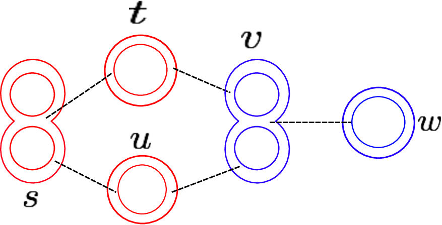
Figure 1: The red double line represents σ\sigma, and the blue double line represents ρ\rho. The dashed line represents a double trace interaction. A vertex in a single color, such as (c) or (d), represents an interaction in Ug​a​u​g​erU_{gauge}^{r}, and thus s≠ts\neq t. A vertex in two colors, such as (e), represents an interaction in Um​a​t​t​e​rrU^{r}_{matter}.

We discuss the calculation of the free energy based on the above Feynman rule. In this calculation, only connected diagrams are relevant as usual. Here, by “connected” we mean that any parts in a diagram are connected by dashed lines or by double lines. Figure 2 shows examples of such diagrams. Since we are interested in the limit (4.4), let us consider what kind of diagrams contributes to the leading order of the 1/N1,21/N_{1,2} expansion. It turns out that the leading contribution is given by the diagrams satisfying the following two conditions:

C​o​n​d​i​t​i​o​n​ 1Condition\ 1.   They are planar with respect to the double lines in the ordinary sense.

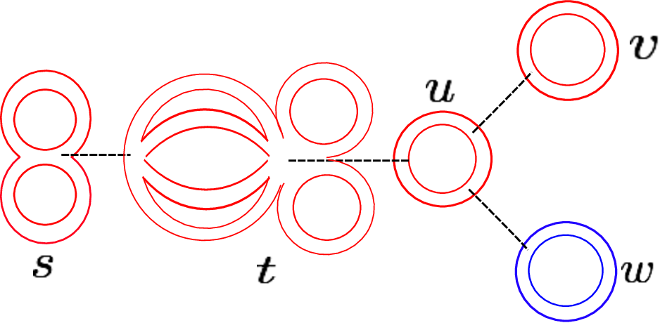
C​o​n​d​i​t​i​o​n​ 2Condition\ 2. They can be separated into two parts by cutting any dashed lines. We call a diagram satisfying the latter condition ‘tree’ diagram since this condition is equivalent to that any dashed lines do not form a loop. We can check the latter condition explicitly for Figure 2(a) as follows. Since N1N_{1} and N2N_{2} are in the same order in the limit (4.4), we denote the order of them collectively by NN. Each propagator gives a factor of N−1N^{-1}, each index loop gives NN and each vertex gives N0N^{0}. While (a) is proportional to N−13×N15=N2N^{-13}\times N^{15}=N^{2}, (b) is proportional to N−12×N12=N0N^{-12}\times N^{12}=N^{0}. Thus, Figure 2(b) does not contribute in the limit (4.4).
Refer to caption
(a) ‘tree’ diagram
Refer to caption
(b) non-‘tree’ diagram
Figure 2: Examples of connected diagrams. While the dashed lines in (a) do not form a loop, the dashed lines in (b) do.

4.2.2 Feynman rule for ABJM matrix model

We next construct the Feynman rule for the ABJM matrix model on S3S^{3}, given by (2.5). This can be written as a manifestly U⁡(N1)×U⁡(N2)U(N_{1})\times U(N_{2}) invariant form as follows,

∫d​σ​𝑑ρ​exp⁡(−N1λ1​tr​σ2+N2λ2​tr​ρ2+Ug​a​u​g​e+Um​a​t​t​e​r),\displaystyle\int d{\sigma}d\rho\exp\Biggl(-\frac{N_{1}}{\lambda_{1}}\mbox{tr}{\sigma}^{2}+\frac{N_{2}}{\lambda_{2}}\mbox{tr}\rho^{2}+{U}_{gauge}+{U}_{matter}\Biggr), (4.22)

where we have defined the ’t Hooft couplings λi\lambda_{i} as 2​π2gs=Niλi\frac{2\pi^{2}}{g_{s}}=\frac{N_{i}}{\lambda_{i}} (i=1,2i=1,2), and Ug​a​u​g​eU_{gauge} and Um​a​t​t​e​rU_{matter} are the double trace interactions,

Ug​a​u​g​e\displaystyle{U}_{gauge} =\displaystyle= −∑a,ba+b∈2​ℕ​2​Ka​b​ζ​(a+b)​(tr​σa​tr​σb+tr​ρa​tr​ρb),\displaystyle-\underset{a+b\in 2\mathbb{N}}{\sum_{a,b}}{2K_{ab}}\ \zeta(a+b)(\mbox{tr}{\sigma}^{a}\ \mbox{tr}{\sigma}^{b}+\mbox{tr}\rho^{a}\ \mbox{tr}\rho^{b}),
Um​a​t​t​e​r\displaystyle{U}_{matter} =\displaystyle= ∑a,ba+b∈2​ℕ​4​Ka​b​ζ​(a+b,12)​tr​σa​tr​ρb.\displaystyle\underset{a+b\in 2\mathbb{N}}{\sum_{a,b}}{4K_{ab}\ \zeta\biggl(a+b,\frac{1}{2}\biggr)}\mbox{tr}{\sigma}^{a}\mbox{tr}\rho^{b}. (4.23)

The vertices in the ABJM matrix model give the following factors,

𝒱(a,b)≡{−4​Ka​b​ζ​(a+b) for ​𝒱(a,b)∈Ug​a​u​g​e4​Ka​b​ζ​(a+b,12) for ​𝒱(a,b)∈Um​a​t​t​e​r.{\mathcal{V}}^{(a,b)}\equiv\begin{cases}-4{K_{ab}}\zeta(a+b)&\text{ for }\ {\mathcal{V}}^{(a,b)}\in U_{gauge}\\ 4{K_{ab}}\zeta(a+b,\frac{1}{2})&\text{ for }\ {\mathcal{V}}^{(a,b)}\in U_{matter}.\end{cases} (4.24)

The relevant diagrams in the limit (4.1) are planar and ‘tree’ as in the case of the reduced model.

Compared with the Feynman rule in the reduced model, the ABJM matrix model does not have the indices s,t,⋯s,t,\cdots in the Feynman diagrams. We will show that after summing over these indices in the reduced model, each diagram in the reduced model reproduces the corresponding diagram in the ABJM matrix model.

4.2.3 Perturbative correspondence of free energy

We compare the free energy of the reduced model with that of the ABJM theory. We will find that, in the limit (4.4), the free energy in the reduced model divided by Λ+1\Lambda+1 coincides with that in the ABJM theory to all orders in the perturbation theory;

ℱr​e​d​u​c​e​dΛ+1=ℱA​B​J​M,\displaystyle\frac{\mathcal{F}_{reduced}}{\Lambda+1}=\mathcal{F}_{ABJM}, (4.25)

under the following identification of the coupling constants,

ti=λi​(i=1,2).\displaystyle t_{i}=\lambda_{i}\ (i=1,2). (4.26)

We note that under (4.26) the coefficients of the gaussian terms of (4.15) and (4.22) coincide and so the factors coming from propagators in the reduced model and the ABJM theory trivially agree for the same Feynman diagrams. Therefore, in the following argument, we ignore the factors of propagators and only take care of the factors coming from vertices in these matrix models.

In the reduced model, any ‘tree’ diagram can be decomposed as

∑s∑tVs​t(a,b)​Rt.\displaystyle\sum_{s}\sum_{t}V^{(a,b)}_{st}R_{t}. (4.27)

Here, Vs​t(a,b)V^{(a,b)}_{st} is an outermost vertex, that is, a vertex on the tip of a branch in the ‘tree’ diagram, and RtR_{t} represents the rest of the diagram. See Figure 3. The explicit form of RtR_{t} for the case shown in Figure 3 is given by (E.1).

Refer to caption
Figure 3: This diagram has three outermost vertices, Vs​t(4,4)V^{(4,4)}_{st}, Vu​v(2,2)V^{(2,2)}_{uv}, Vu​w(2,2)V^{(2,2)}_{uw}. Here, we have separated Vs​t(4,4)V_{st}^{(4,4)} from the shaded part, RtR_{t}.

We will show that in the Λ→∞\Lambda\rightarrow\infty limit, we can replace the sum ∑sVs​t(a,b)\sum_{s}V^{(a,b)}_{st} in (4.27) by the corresponding vertex in the ABJM theory. That is,

limΛ→∞1Λ+1​∑t∑sVs​t(a,b)​Rt=limΛ→∞𝒱(a,b)Λ+1​∑tRt,\displaystyle\lim_{\Lambda\rightarrow\infty}\frac{1}{\Lambda+1}\sum_{t}\sum_{s}V_{st}^{(a,b)}R_{t}=\lim_{\Lambda\rightarrow\infty}\frac{{\mathcal{V}}^{(a,b)}}{\Lambda+1}\sum_{t}R_{t}, (4.28)

where 𝒱(a,b)\mathcal{V}^{(a,b)} in the right-hand side is given by 𝒱(a,b)∈Ug​a​u​g​e\mathcal{V}^{(a,b)}\in U_{gauge} when Vs​t(a,b)∈Ug​a​u​g​er{V}_{st}^{(a,b)}\in U^{r}_{gauge} and by 𝒱(a,b)∈Um​a​t​t​e​r\mathcal{V}^{(a,b)}\in U_{matter} when Vs​t(a,b)∈Um​a​t​t​e​rr{V}_{st}^{(a,b)}\in U^{r}_{matter}. If we establish (4.28), by repeatedly replacing the vertices of the reduced model by those of the ABJM theory, the factor coming from vertices in the reduced model agrees exactly with that in the Aharony-Bergman-Jafferis-Maldacena(ABJM) matrix model. For an illustration of this procedure, see Figure 4. Since this equivalence holds for all the ‘tree’ diagrams, we thus establish the perturbative equivalence of the free energy between the reduced model and the ABJM theory (4.25).
Refer to caption
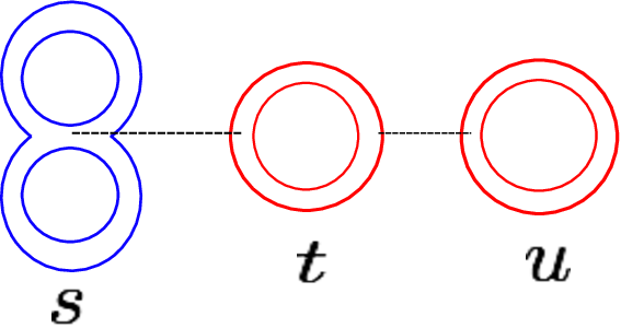
Figure 4: The vertices in this diagram give a factor 1Λ+1​∑s,t,uVs​t(2,4)​Vt​u(2,2)\frac{1}{\Lambda+1}\sum_{s,t,u}V^{(2,4)}_{st}V^{(2,2)}_{tu}, where Vs​t(2,4)∈Um​a​t​t​e​rrV^{(2,4)}_{st}\in U_{matter}^{r} and Vt​u(2,4)∈Ug​a​u​g​erV_{tu}^{(2,4)}\in U_{gauge}^{r}. By (4.28), in the Λ→∞\Lambda\rightarrow\infty limit this is equal to 𝒱(2,4)​𝒱(2,2)​1Λ+1​∑u1=𝒱(2,4)​𝒱(2,2){\mathcal{V}}^{(2,4)}{\mathcal{V}}^{(2,2)}\frac{1}{\Lambda+1}\sum_{u}1={\mathcal{V}}^{(2,4)}{\mathcal{V}}^{(2,2)}, and thus we can recover the factor of the corresponding vertices in the ABJM theory.

We now prove (4.28). For the vertex Vs​t(a,b)∈Um​a​t​t​e​rrV^{(a,b)}_{st}\in U_{matter}^{r}, the left-hand side in (4.28) is calculated as

limΛ→∞1Λ+1​∑t=−Λ2Λ2∑s=−Λ2(s≠t)Λ2−2​Ka​b(s−t)a+b​Rt\displaystyle\lim_{\Lambda\rightarrow\infty}\frac{1}{\Lambda+1}\sum_{t=-\frac{\Lambda}{2}}^{\frac{\Lambda}{2}}\sum_{\begin{subarray}{c}s=-\frac{\Lambda}{2}\\ (s\neq t)\end{subarray}}^{\frac{\Lambda}{2}}\frac{-2K_{ab}}{(s-t)^{a+b}}R_{t}
=limΛ→∞−2Λ+1​∑t=−Λ2Λ2Ka​b​Rt​(2​ζ​(a+b)−ζ⁡(a+b,Λ2+t+1)−ζ⁡(a+b,Λ2−t+1)).\displaystyle=\lim_{\Lambda\rightarrow\infty}\frac{-2}{\Lambda+1}\sum_{t=-\frac{\Lambda}{2}}^{\frac{\Lambda}{2}}K_{ab}R_{t}\Biggl(2\zeta(a+b)-\zeta\biggl(a+b,\frac{\Lambda}{2}+t+1\biggr)-\zeta\biggl(a+b,\frac{\Lambda}{2}-t+1\biggr)\Biggr). (4.29)

The first term above agrees with the right-hand side in (4.28). The remaining terms vanish in the Λ→∞\Lambda\rightarrow\infty limit. To see this, we use the fact that |Rt||R_{t}| has a Λ\Lambda-independent upper bound denoted by CC, which we prove in appendix E. By using this fact, the absolute value of the remaining terms is bounded from above by

limΛ→∞2​|Ka​b|​CΛ+1​∑t=−Λ2Λ2(ζ⁡(a+b,Λ2+t+1)+ζ⁡(a+b,Λ2−t+1))\displaystyle\lim_{\Lambda\rightarrow\infty}\frac{2|K_{ab}|C}{\Lambda+1}\sum_{t=-\frac{\Lambda}{2}}^{\frac{\Lambda}{2}}\Biggl(\zeta\biggl(a+b,\frac{\Lambda}{2}+t+1\biggr)+\zeta\biggl(a+b,\frac{\Lambda}{2}-t+1\biggr)\Biggr) (4.30)
=\displaystyle= 4​|Ka​b|​C​limΛ→∞1Λ+1​(∑n=0Λ1(n+1)a+b−1+∑m=Λ+1∞Λ+1(m+1)a+b)=0,\displaystyle 4|K_{ab}|C\lim_{\Lambda\rightarrow\infty}\frac{1}{\Lambda+1}\biggl(\sum_{n=0}^{\Lambda}\frac{1}{(n+1)^{a+b-1}}+\sum_{m=\Lambda+1}^{\infty}\frac{\Lambda+1}{(m+1)^{a+b}}\biggr)=0,

where we have used the definition of the generalized zeta function (4.14). The terms in the second line are 𝒪⁡(log⁡Λ/Λ)\mathcal{O}(\log\Lambda/\Lambda) for a+b=2a+b=2, and 𝒪⁡(1/Λ)\mathcal{O}(1/\Lambda) for a+b>2a+b>2.

For the vertex Vs​t(a,b)∈Um​a​t​t​e​rrV^{(a,b)}_{st}\in U_{matter}^{r}, the left-hand side in (4.28) is calculated as,

1Λ+1​∑t=−Λ2Λ2∑s=−Λ2Λ24​Ka​b2a+b​(ζ⁡(a+b,14+|s−t|2)−ζ⁡(a+b,34+|s−t|2))​Rt\displaystyle\frac{1}{\Lambda+1}\sum_{t=-\frac{\Lambda}{2}}^{\frac{\Lambda}{2}}\sum_{s=-\frac{\Lambda}{2}}^{\frac{\Lambda}{2}}\frac{4K_{ab}}{2^{a+b}}\Biggl(\zeta\biggl(a+b,\frac{1}{4}+\frac{|s-t|}{2}\biggr)-\zeta\biggl(a+b,\frac{3}{4}+\frac{|s-t|}{2}\biggr)\Biggr)R_{t}
=1Λ+1​∑t=−Λ2Λ24​Ka​b2a+b​(2a+b​ζ​(a+b,12)−ζ⁡(a+b,14+Λ2+t2)−ζ⁡(a+b,34+Λ2−t2))​Rt,\displaystyle=\frac{1}{\Lambda+1}\sum_{t=-\frac{\Lambda}{2}}^{\frac{\Lambda}{2}}\frac{4K_{ab}}{2^{a+b}}\Biggl(2^{a+b}\zeta\biggl(a+b,\frac{1}{2}\biggr)-\zeta\biggl(a+b,\frac{1}{4}+\frac{\frac{\Lambda}{2}+t}{2}\biggr)-\zeta\biggl(a+b,\frac{3}{4}+\frac{\frac{\Lambda}{2}-t}{2}\biggr)\Biggr)R_{t}, (4.31)

where we have used the equality, ζ⁡(a+b,14)+ζ⁡(a+b,34)=2a+b​ζ​(a+b,12)\zeta(a+b,\frac{1}{4})+\zeta(a+b,\frac{3}{4})=2^{a+b}\zeta(a+b,\frac{1}{2}). The first term in (4.31) agrees with the right-hand side in (4.28). The remaining terms vanish in the Λ→∞\Lambda\rightarrow\infty limit, which can be shown in the same way as (4.30). Therefore, the equality (4.28) has been proved.

Here, we briefly comment on the cutoff effect of Λ\Lambda. For this purpose, we consider the one-point function ⟨tr​σs2⟩\langle\mbox{tr}{\sigma}_{s}^{2}\rangle for a fixed s∈{−Λ2,⋯,Λ2}s\in\{-\frac{\Lambda}{2},\cdots,\frac{\Lambda}{2}\}. Figure 5(a) is one of the diagrams which contributes to the one-point function, and leads to the following factor

∑u(≠s)1(s−u)4=(∑n=1Λ2−s+∑n=1s+Λ2)1n4.\displaystyle\sum_{u(\neq s)}\frac{1}{(s-u)^{4}}=\biggl(\sum_{n=1}^{\frac{\Lambda}{2}-s}+\sum_{n=1}^{s+\frac{\Lambda}{2}}\biggr)\frac{1}{n^{4}}. (4.32)

In the Λ→∞\Lambda\rightarrow\infty limit, while (4.32) goes to 2​ζ​(4)2\,\zeta(4) for all s∈{−Λ2+𝒪⁡(ln⁡Λ),⋯,Λ2−𝒪⁡(ln⁡Λ)}s\in\{-\frac{\Lambda}{2}+\mathcal{O}(\ln\Lambda),\cdots,\frac{\Lambda}{2}-\mathcal{O}(\ln\Lambda)\}, it deviates from 2​ζ​(4)2\,\zeta(4) for ss with |s±Λ2|∼𝒪⁡(Λ0)|s\pm\frac{\Lambda}{2}|\sim\mathcal{O}(\Lambda^{0}). Therefore, although (4.32) depends on the value of ss, the dependence is negligible for almost all ss except near the cutoff ±Λ2\pm\frac{\Lambda}{2}, and only ss within 𝒪⁡(Λ0)\mathcal{O}(\Lambda^{0}) from the boundaries feels the cutoff effect (See Figure 5(b)). Note that this argument also holds for more general diagrams. Thus, the number of the modes affected by the cutoff is 𝒪⁡(Λ0)\mathcal{O}(\Lambda^{0}), which is negligible compared to the total number, Λ+1\Lambda+1. Since the free energy and one-point functions of Wilson loops are written as an average value over various ss, the cutoff effect is negligible in the Λ→∞\Lambda\rightarrow\infty limit.

Refer to caption
(a)

Refer to caption
(b)
Figure 5: Figure (a): A diagram contributing to ⟨tr​σs2⟩\langle\mbox{tr}{\sigma}_{s}^{2}\rangle. Figure (b) : Only ss near ±Λ2\pm\frac{\Lambda}{2} feels the cutoff effect.

4.2.4 Perturbative correspondence of Wilson loop

We can easily prove the perturbative equivalence between the Wilson loop in the reduced model and that in the ABJM matrix model. While the Wilson loop in the ABJM theory is given by (2.8), the corresponding object in the reduced model is obtained by applying the representation (4.2) to (3.46). Therefore, what we want to show is

1N1​⟨tr​e2​π​σ⟩=1N1​(Λ+1)​∑s=−Λ2Λ2⟨tr​e2​π​σs⟩,\displaystyle\frac{1}{N_{1}}\langle\mbox{tr}e^{2\pi{\sigma}}\rangle=\frac{1}{N_{1}(\Lambda+1)}\sum_{s=-\frac{\Lambda}{2}}^{\frac{\Lambda}{2}}\langle\mbox{tr}e^{2\pi{\sigma}_{s}}\rangle, (4.33)

where the ⟨⋯⟩\langle\cdots\rangle means the average with respect to the eigenvalue integral of each theory. In perturbation theory, both of the left-hand side and the right-hand side above are calculated by expanding the exponentials. Thus, (4.33) holds if we have, for any positive integer aa,

⟨tr​σa⟩=1Λ+1​∑s=−Λ2Λ2⟨tr​σsa⟩.\displaystyle\langle\mbox{tr}{\sigma}^{a}\rangle=\frac{1}{\Lambda+1}\sum_{s=-\frac{\Lambda}{2}}^{\frac{\Lambda}{2}}\langle\mbox{tr}{\sigma}^{a}_{s}\rangle. (4.34)

We find that this is true from (4.28), and so is (4.33).

4.3 Large-NN equivalence of eigenvalue density

In this section, we investigate the eigenvalue distributions of σs\sigma_{s} and ρs\rho_{s} in the reduced model for the ABJM matrix model. We show that if ss is sufficiently apart from the cutoff ±Λ/2\pm\Lambda/2 the eigenvalue densities of σs\sigma_{s} and ρs\rho_{s} coincide with those of σ\sigma and ρ\rho in the ABJM matrix model, respectively, and thereby prove the large-NN equivalence between the reduced model and the original ABJM theory.

We start with the ABJM matrix model (2.5). From (2.5), the effective action for the eigenvalues are read off as

Seff\displaystyle S_{\mathrm{eff}} =N1λ1​∑iσi2−N2λ2​∑αρα2−12​∑i≠jln⁡sinh2⁡{π⁡(σi−σj)}−12​∑α≠βln⁡sinh2⁡{π⁡(ρα−ρα)}\displaystyle=\frac{N_{1}}{\lambda_{1}}\sum_{i}\sigma_{i}^{2}-\frac{N_{2}}{\lambda_{2}}\sum_{\alpha}\rho_{\alpha}^{2}-\frac{1}{2}\sum_{i\neq j}\ln\sinh^{2}\{\pi(\sigma_{i}-\sigma_{j})\}-\frac{1}{2}\sum_{\alpha\neq\beta}\ln\sinh^{2}\{\pi(\rho_{\alpha}-\rho_{\alpha})\}
+2∑i,αlncosh{π(σi−ρα)}.\displaystyle\quad+2\sum_{i,\alpha}\ln\cosh\{\pi(\sigma_{i}-\rho_{\alpha})\}. (4.35)

Varying SeffS_{\mathrm{eff}} with respect to σi\sigma_{i} and ρα\rho_{\alpha}, we obtain the saddle point equation

0\displaystyle 0 =N1π​λ1​σi−∑j(≠i)coth⁡{π⁡(σi−σj)}+∑αtanh⁡{π⁡(σi−ρα)},\displaystyle=\frac{N_{1}}{\pi\lambda_{1}}\sigma_{i}-\sum_{j(\neq i)}\coth\{\pi(\sigma_{i}-\sigma_{j})\}+\sum_{\alpha}\tanh\{\pi(\sigma_{i}-\rho_{\alpha})\},
0\displaystyle 0 =−N2π​λ2​ρα−∑β(≠α)coth⁡{π⁡(ρα−ρβ)}−∑itanh⁡{π⁡(σi−ρα)}.\displaystyle=-\frac{N_{2}}{\pi\lambda_{2}}\rho_{\alpha}-\sum_{\beta(\neq\alpha)}\coth\{\pi(\rho_{\alpha}-\rho_{\beta})\}-\sum_{i}\tanh\{\pi(\sigma_{i}-\rho_{\alpha})\}. (4.36)

Let us introduce the eigenvalue densities for σi\sigma_{i} and ρα\rho_{\alpha} as

ρ⁡(x)=1N1​∑i=1N1δ⁡(x−σi),ρ~​(x)\displaystyle\rho(x)=\frac{1}{N_{1}}\sum_{i=1}^{N_{1}}\delta(x-\sigma_{i}),\;\;\;\tilde{\rho}(x) =1N2​∑α=1N2δ⁡(x−ρα).\displaystyle=\frac{1}{N_{2}}\sum_{\alpha=1}^{N_{2}}\delta(x-\rho_{\alpha}). (4.37)

Using these we can rewrite the saddle point equations as

0=\displaystyle 0= 1π​λ1x−−∫dycoth{π(x−y)}ρ(y)+N2N1∫dytanh{π(x−y)}ρ~(y),\displaystyle\frac{1}{\pi\lambda_{1}}x-\mathchoice{{\vbox{\hbox{$\textstyle-$}}\kern-4.86108pt}}{{\vbox{\hbox{$\scriptstyle-$}}\kern-3.43057pt}}{{\vbox{\hbox{$\scriptscriptstyle-$}}\kern-2.908pt}}{{\vbox{\hbox{$\scriptscriptstyle-$}}\kern-2.76045pt}}\!\int dy\coth\{\pi(x-y)\}\ \rho(y)+\frac{N_{2}}{N_{1}}\int dy\tanh\{\pi(x-y)\}\ \tilde{\rho}(y),
0=\displaystyle 0= −1π​λ2x−−∫dycoth{π(x−y)}ρ~(y)+N1N2∫dytanh{π(x−y)}ρ(y),\displaystyle-\frac{1}{\pi\lambda_{2}}x-\mathchoice{{\vbox{\hbox{$\textstyle-$}}\kern-4.86108pt}}{{\vbox{\hbox{$\scriptstyle-$}}\kern-3.43057pt}}{{\vbox{\hbox{$\scriptscriptstyle-$}}\kern-2.908pt}}{{\vbox{\hbox{$\scriptscriptstyle-$}}\kern-2.76045pt}}\!\int dy\coth\{\pi(x-y)\}\ \tilde{\rho}(y)+\frac{N_{1}}{N_{2}}\int dy\tanh\{\pi(x-y)\}\ \rho(y), (4.38)

where −⁣∫\mathchoice{{\vbox{\hbox{$\textstyle-$}}\kern-4.86108pt}}{{\vbox{\hbox{$\scriptstyle-$}}\kern-3.43057pt}}{{\vbox{\hbox{$\scriptscriptstyle-$}}\kern-2.908pt}}{{\vbox{\hbox{$\scriptscriptstyle-$}}\kern-2.76045pt}}\!\int represents the Cauchy principal integral. In the large-NN limit (4.1), the eigenvalues obeying (4.38) form a continuous distribution and so the eigenvalue densities become smooth functions. The explicit solution of (4.38) can be found in [3, 45].

Next let us consider our reduced model (4.6) for the ABJM theory. The effective action for the eigenvalues σs​i\sigma_{si} and ρs​i\rho_{si} is given by

Seff\displaystyle S_{\mathrm{eff}} =N1t1​∑s​iσs​i2−N2t2​∑s​αρs​α2−12​∑s∑i≠jln⁡(σs​i−σs​j)2−12​∑s∑α≠βln⁡(ρs​α−ρs​β)2\displaystyle=\frac{N_{1}}{t_{1}}\sum_{si}\sigma_{si}^{2}-\frac{N_{2}}{t_{2}}\sum_{s\alpha}\rho_{s\alpha}^{2}-\frac{1}{2}\sum_{s}\sum_{i\neq j}\ln(\sigma_{si}-\sigma_{sj})^{2}-\frac{1}{2}\sum_{s}\sum_{\alpha\neq\beta}\ln(\rho_{s\alpha}-\rho_{s\beta})^{2}
−12∑s≠t∑i,jln{1+(σs​i−σt​j)2(s−t)2}−12∑s≠t∑α,βln{1+(ρs​α−ρt​β)2(s−t)2}\displaystyle-\frac{1}{2}\sum_{s\neq t}\sum_{i,j}\ln\left\{1+\frac{(\sigma_{si}-\sigma_{tj})^{2}}{(s-t)^{2}}\right\}-\frac{1}{2}\sum_{s\neq t}\sum_{\alpha,\beta}\ln\left\{1+\frac{(\rho_{s\alpha}-\rho_{t\beta})^{2}}{(s-t)^{2}}\right\}
−2∑s,t∑i,α∑J=|s−t|/2∞[ln{(2J+32)2+(σs​i−ρt​α)2}−ln{(2J+12)2+(σs​i−ρt​α)2}],\displaystyle-2\sum_{s,t}\sum_{i,\alpha}\sum_{J=|s-t|/2}^{\infty}\left[\ln\left\{\left(2J+\frac{3}{2}\right)^{2}+(\sigma_{si}-\rho_{t\alpha})^{2}\right\}-\ln\left\{\left(2J+\frac{1}{2}\right)^{2}+(\sigma_{si}-\rho_{t\alpha})^{2}\right\}\right], (4.39)

where the summation of s,ts,t is taken over s,t=−Λ/2,⋯,Λ/2s,t=-\Lambda/2,\cdots,\Lambda/2. The saddle point equations are

0\displaystyle 0 =N1t1​σs​i−∑j(≠i)1σs​i−σs​j−∑t(≠s)∑jσs​i−σt​j(s−t)2+(σs​i−σt​j)2\displaystyle=\frac{N_{1}}{t_{1}}\sigma_{si}-\sum_{j(\neq i)}\frac{1}{\sigma_{si}-\sigma_{sj}}-\sum_{t(\neq s)}\sum_{j}\frac{\sigma_{si}-\sigma_{tj}}{(s-t)^{2}+(\sigma_{si}-\sigma_{tj})^{2}}
−2∑t,α∑J=|s−t|/2∞[σs​i−ρt​α(2​J+32)2+(σs​i−ρt​α)2−σs​i−ρt​α(2​J+12)2+(σs​i−ρt​α)2],\displaystyle-2\sum_{t,\alpha}\sum_{J=|s-t|/2}^{\infty}\left[\frac{\sigma_{si}-\rho_{t\alpha}}{\left(2J+\frac{3}{2}\right)^{2}+(\sigma_{si}-\rho_{t\alpha})^{2}}-\frac{\sigma_{si}-\rho_{t\alpha}}{\left(2J+\frac{1}{2}\right)^{2}+(\sigma_{si}-\rho_{t\alpha})^{2}}\right],
0\displaystyle 0 =−N2t2​ρs​α−∑β(≠α)1ρs​α−ρs​β−∑t(≠s)∑βρs​α−ρs​β(s−t)2+(ρs​α−ρt​β)2\displaystyle=-\frac{N_{2}}{t_{2}}\rho_{s\alpha}-\sum_{\beta(\neq\alpha)}\frac{1}{\rho_{s\alpha}-\rho_{s\beta}}-\sum_{t(\neq s)}\sum_{\beta}\frac{\rho_{s\alpha}-\rho_{s\beta}}{(s-t)^{2}+(\rho_{s\alpha}-\rho_{t\beta})^{2}}
+2∑t,i∑J=|s−t|/2∞[σt​i−ρs​α(2​J+32)2+(σt​i−ρs​α)2−σt​i−ρs​α(2​J+12)2+(σt​i−ρs​α)2].\displaystyle+2\sum_{t,i}\sum_{J=|s-t|/2}^{\infty}\left[\frac{\sigma_{ti}-\rho_{s\alpha}}{\left(2J+\frac{3}{2}\right)^{2}+(\sigma_{ti}-\rho_{s\alpha})^{2}}-\frac{\sigma_{ti}-\rho_{s\alpha}}{\left(2J+\frac{1}{2}\right)^{2}+(\sigma_{ti}-\rho_{s\alpha})^{2}}\right]. (4.40)

We introduce the eigenvalue densities of σs\sigma_{s} and ρs\rho_{s} in the reduced model as

ρ[s]​(x)=1N1​∑i=1N1δ⁡(x−σs​i),ρ~[s]​(x)\displaystyle\rho^{[s]}(x)=\frac{1}{N_{1}}\sum_{i=1}^{N_{1}}\delta(x-\sigma_{si}),\;\;\;\tilde{\rho}^{[s]}(x) =1N2​∑α=1N2δ⁡(x−ρs​α),\displaystyle=\frac{1}{N_{2}}\sum_{\alpha=1}^{N_{2}}\delta(x-\rho_{s\alpha}), (4.41)

and rewrite (4.40) as

0\displaystyle 0 =1t1​x−−∫d​y​1x−y​ρ[s]​(y)−∑t(≠s)∫d​y​x−y(s−t)2+(x−y)2​ρ[t]​(y)\displaystyle=\frac{1}{t_{1}}x-\mathchoice{{\vbox{\hbox{$\textstyle-$}}\kern-4.86108pt}}{{\vbox{\hbox{$\scriptstyle-$}}\kern-3.43057pt}}{{\vbox{\hbox{$\scriptscriptstyle-$}}\kern-2.908pt}}{{\vbox{\hbox{$\scriptscriptstyle-$}}\kern-2.76045pt}}\!\int dy\frac{1}{x-y}\rho^{[s]}(y)-\sum_{t(\neq s)}\int dy\frac{x-y}{(s-t)^{2}+(x-y)^{2}}\rho^{[t]}(y)
−2​N2N1∑t∑J=|s−t|/2∞∫dy[x−y(2​J+32)2+(x−y)2−x−y(2​J+12)2+(x−y)2]ρ~[t](y),\displaystyle-\frac{2N_{2}}{N_{1}}\sum_{t}\sum_{J=|s-t|/2}^{\infty}\int dy\left[\frac{x-y}{\left(2J+\frac{3}{2}\right)^{2}+(x-y)^{2}}-\frac{x-y}{\left(2J+\frac{1}{2}\right)^{2}+(x-y)^{2}}\right]\tilde{\rho}^{[t]}(y),
0\displaystyle 0 =−1t2​x−−∫d​y​1x−y​ρ~[s]​(y)−∑t(≠s)∫d​y​x−y(s−t)2+(x−y)2​ρ~[t]​(y)\displaystyle=-\frac{1}{t_{2}}x-\mathchoice{{\vbox{\hbox{$\textstyle-$}}\kern-4.86108pt}}{{\vbox{\hbox{$\scriptstyle-$}}\kern-3.43057pt}}{{\vbox{\hbox{$\scriptscriptstyle-$}}\kern-2.908pt}}{{\vbox{\hbox{$\scriptscriptstyle-$}}\kern-2.76045pt}}\!\int dy\frac{1}{x-y}\tilde{\rho}^{[s]}(y)-\sum_{t(\neq s)}\int dy\frac{x-y}{(s-t)^{2}+(x-y)^{2}}\tilde{\rho}^{[t]}(y)
−2​N1N2∑t∑J=|s−t|/2∞∫dy[x−y(2​J+32)2+(x−y)2−x−y(2​J+12)2+(x−y)2]ρ[t](y).\displaystyle-\frac{2N_{1}}{N_{2}}\sum_{t}\sum_{J=|s-t|/2}^{\infty}\int dy\left[\frac{x-y}{\left(2J+\frac{3}{2}\right)^{2}+(x-y)^{2}}-\frac{x-y}{\left(2J+\frac{1}{2}\right)^{2}+(x-y)^{2}}\right]\rho^{[t]}(y). (4.42)

We can find a solution to these equations in the Λ→∞\Lambda\rightarrow\infty limit as follows. If one naively takes the Λ→∞\Lambda\rightarrow\infty limit in (4.42), (ρ[s]​(x),ρ~[s]​(x))=(ρ⁡(x),ρ~​(x))(\rho^{[s]}(x),\tilde{\rho}^{[s]}(x))=(\rho(x),\tilde{\rho}(x)) with λ1=t1\lambda_{1}=t_{1} and λ2=t2\lambda_{2}=t_{2} for arbitrary ss turns out to be a solution to (4.42), where (ρ​(x),ρ~​(x))(\rho(x),\tilde{\rho}(x)) is the solution to the saddle point equation (4.38) of the ABJM matrix model. This is because in this case (4.42) reduces to (4.38) (see appendix F.1). This solution represents infinitely many copies of that of the original ABJM matrix model. Since the free energy and the Wilson loop in the reduced model are given by an average over all ss’s as (4.25) and (4.33), they exactly coincide with those in the ABJM matrix model.

The densities (ρ[s]​(x),ρ~[s]​(x))(\rho^{[s]}(x),\tilde{\rho}^{[s]}(x)) with ss near the cutoff Λ\Lambda deviate from (ρ​(x),ρ~​(x))(\rho(x),\tilde{\rho}(x)). This cutoff effect would spoil the above naive argument if the correlation range between ρ[s]\rho^{[s]}’s and ρ~[s]\tilde{\rho}^{[s]}’s became larger as 𝒪⁡(Λ)\mathcal{O}(\Lambda). In this case, the number of (ρ[s]​(x),ρ~[s]​(x))(\rho^{[s]}(x),\tilde{\rho}^{[s]}(x)) which deviates from (ρ​(x),ρ~​(x))(\rho(x),\tilde{\rho}(x)) would be 𝒪⁡(Λ)\mathcal{O}(\Lambda), namely, the number of the deviating densities and that of the densities coinciding with (ρ​(x),ρ~​(x))(\rho(x),\tilde{\rho}(x)) would become comparable. Then the free energy and the Wilson loop in the reduced model given by the average over ss’s would not coincide with those in the original model.

However, this is not the case of our reduced model. It turns out that the correlation range is 𝒪⁡(Λ0)\mathcal{O}(\Lambda^{0}), and so the above naive argument is indeed valid. In fact, in the saddle point equation for ρ[s]​(x)\rho^{[s]}(x) (or ρ~[s]​(x)\tilde{\rho}^{[s]}(x)), the coefficients of ρ[t]​(x)\rho^{[t]}(x) and ρ~[t]​(x)\tilde{\rho}^{[t]}(x) are suppressed if |t−s||t-s| is large enough. As shown in appendix F.2, the contributions from the terms with |t−s|≥ln⁡Λ|t-s|\geq\ln\Lambda can be neglected in the Λ→∞\Lambda\rightarrow\infty limit. Namely, the profile of ρ[s]​(x)\rho^{[s]}(x) (or ρ~[s]​(x)\tilde{\rho}^{[s]}(x)) is determined only by (ρ[t]​(x),ρ~[t]​(x))(\rho^{[t]}(x),\tilde{\rho}^{[t]}(x))’s with |t−s|≲𝒪⁡(Λ0)|t-s|\lesssim{\cal O}(\Lambda^{0}), which means that the correlation range is sufficiently small compared to the system size Λ\Lambda, so that (ρ[s]​(x),ρ~[s]​(x))(\rho^{[s]}(x),\tilde{\rho}^{[s]}(x)) for |s|≲Λ/2−ln⁡Λ|s|\lesssim\Lambda/2-\ln\Lambda are not affected by the cutoff. Therefore, in the Λ→∞\Lambda\rightarrow\infty limit (ρ[s]​(x),ρ~[s]​(x))=(ρ⁡(x),ρ~​(x))(\rho^{[s]}(x),\tilde{\rho}^{[s]}(x))=(\rho(x),\tilde{\rho}(x)) still holds except for very narrow region Λ/2−ln⁡Λ≲|s|≤Λ/2\Lambda/2-\ln\Lambda\lesssim|s|\leq\Lambda/2. This is consistent with our observation in the perturbation theory mentioned in the last part of section 4.2.3. Also this behavior of the densities is observed in the numerical simulation for the reduced model of the pure CS theory on S3S^{3} [41]. Although (ρ[s]​(x),ρ~[s]​(x))(\rho^{[s]}(x),\tilde{\rho}^{[s]}(x)) for Λ/2−ln⁡Λ≲|s|≤Λ/2\Lambda/2-\ln\Lambda\lesssim|s|\leq\Lambda/2 differs from (ρ​(x),ρ~​(x))(\rho(x),\tilde{\rho}(x)), their contributions to the physical quantities, such as the free energy and the BPS Wilson loops, are negligible since the physical quantities are calculated as an average taken over all ss’s.

Thus, for supersymmetric observables, the large-NN equivalence between the reduced model and the ABJM theory is also shown non-perturbatively through the saddle point method of the eigenvalue density. One can also apply the saddle point analysis to general 𝒩=2\mathcal{N}=2 non-chiral quiver CS theories and show the large-NN equivalence.

5 Conclusion

In this paper, we have studied the large-NN reduction for a general 𝒩=2{\cal N}=2 non-chiral quiver CS theory on S3S^{3}. We considered the reduced model of the ABJM theory on S3S^{3} as an illustration and explained the calculation of the free energy and the one-point function of the BPS Wilson loop operator in the reduced model. We found that the localization technique reduces the calculation to eigenvalue integrals, as in the original theory on S3S^{3}. To establish the large-NN equivalence, we first studied the integrals in the perturbation theory. We constructed the Feynman rule from the eigenvalue integrals, and found that each Feynman diagram in the reduced model coincides with a corresponding diagram in the ABJM matrix model in the continuum limit. Hence, we conclude that these supersymmetric quantities are equivalent in two theories to all orders in the perturbative expansion. Then we considered the saddle point configuration of the eigenvalues in the reduced model. We found that in the continuum limit the cutoff effect is sufficiently small and that the eigenvalue densities in the reduced model at the saddle point consist of infinitely many copies of those in the original theory. This implies that the expectation values of supersymmetric observables in the reduced model, which are written as the average over all the copies, agree with those in the original theory in the continuum limit. Thus the large-NN equivalence holds also non-perturbatively. Our result gives a strong evidence that the non-perturbative formulation for supersymmetric theories based on the novel large-NN reduction works successfully.

Acknowledgements

The work of G.I. and T.O. is supported by the Grant-in-Aid for the Global COE Program “The Next Generation of Physics, Spun from Universality and Emergence” from the Ministry of Education, Culture, Sports, Science and Technology (MEXT) of Japan. The work of S.S. is supported in part by the JSPS Research Fellowship for Young Scientists.

Appendix A 𝒩=2{\cal N}=2 quiver CS theory on S3S^{3}

In this appendix, we summarize our convention for 𝒩=2\mathcal{N}=2 quiver CS theory on S3S^{3} [5]. We consider the gauge vector multiplet and the matter chiral multiplets in the adjoint and in the bifundamental representation.

A gauge multiplet contains fermionic (Grassmaniann) fields {λ,λ¯}\{\lambda,\bar{\lambda}\} as well as bosonic fields {Aμ,σ,D}\{A_{\mu},\sigma,D\}. There are two kinds of supersymmetric action for this multiplet: the CS action and the YM action, which are defined by

SC​S=−∫dx3tr[εμ​ν​λ(Aμ∂νAλ−2​i3AμAνAλ)+g(−λ¯λ+2Dσ)],\displaystyle S_{CS}=-\int{d}{{}^{3}x}\;\mbox{tr}\!\!\left[\varepsilon^{\mu\nu\lambda}(A_{\mu}\partial_{\nu}A_{\lambda}-\frac{2i}{3}A_{\mu}A_{\nu}A_{\lambda})+\sqrt{g}(-\bar{\lambda}\lambda+2D\sigma)\right], (A.1)
SY​M=∫d3​x​g​tr​[14​Fμ​ν​Fμ​ν+12​(σ+D)2+12​(Dμ​σ)2+i2​λ¯​γμ​Dμ​λ−14​λ¯​λ+i2​λ¯​[σ,λ]].\displaystyle S_{YM}=\int d^{3}x\sqrt{g}\;\mbox{tr}\Big[\frac{1}{4}F^{\mu\nu}F_{\mu\nu}+\frac{1}{2}(\sigma+D)^{2}+\frac{1}{2}(D_{\mu}\sigma)^{2}+\frac{i}{2}\bar{\lambda}\gamma^{\mu}D_{\mu}\lambda-\frac{1}{4}\bar{\lambda}\lambda+\frac{i}{2}\bar{\lambda}[\sigma,\lambda]\Big]. (A.2)

The field strength is defined as usual by Fμ​ν=∂μAν−∂νAμ−i⁡[Aμ,Aν]F_{\mu\nu}=\partial_{\mu}A_{\nu}-\partial_{\nu}A_{\mu}-i[A_{\mu},A_{\nu}], and the covariant derivative contains the gauge and the spin connections,

Dμ​λ=∂μλ+14​ωμb​c​γb​c​λ−i⁡[Aμ,λ].\displaystyle D_{\mu}\lambda=\partial_{\mu}\lambda+\frac{1}{4}\omega_{\mu}^{\;\;bc}\gamma_{bc}\lambda-i[A_{\mu},\lambda]. (A.3)

A matter multiplet in the bifundamental representation consists of bosonic fields {ϕ,ϕ¯,F,F¯}\{\phi,\bar{\phi},F,\bar{F}\} and fermionic fields {ψ,ψ¯}\{\psi,\bar{\psi}\}. We assume that they couple to a gauge multiplet {Aμ,λ,σ,D}\{A_{\mu},\lambda,\sigma,D\} as the fundamental representation and to another gauge multiplet {Bμ,η,ρ,D~}\{B_{\mu},\eta,\rho,\tilde{D}\} as the anti-fundamental. The supersymmetric action for this multiplet is given by99 9 In general, the theory may have a superpotential. We ignore it in this paper since it is irrelevant for the localization calculation.

Sm​a​t​t​e​r=∫d3xgtr[Dμϕ¯Dμϕ−iψ¯γμDμψ+q(2−q)ϕ¯ϕ−2​q−12ψ¯ψ+i(2q−1)ϕ¯∇(σ,ρ)ϕ\displaystyle S_{matter}=\int d^{3}x\sqrt{g}\;\mbox{tr}[D^{\mu}\bar{\phi}D_{\mu}\phi-i\bar{\psi}\gamma^{\mu}D_{\mu}\psi+q(2-q)\bar{\phi}\phi-\frac{2q-1}{2}\bar{\psi}\psi+i(2q-1)\bar{\phi}\nabla(\sigma,\rho)\phi
+iψ¯∇(σ,ρ)ψ+iψ¯∇(λ,η)ϕ−iϕ¯∇(λ¯,η¯)ψ+iϕ¯∇(D,D~)ϕ+ϕ¯∇(σ,ρ)2ϕ+F¯F].\displaystyle\;+i\bar{\psi}\nabla(\sigma,\rho)\psi+i\bar{\psi}\nabla(\lambda,\eta)\phi-i\bar{\phi}\nabla(\bar{\lambda},\bar{\eta})\psi+i\bar{\phi}\nabla(D,\tilde{D})\phi+\bar{\phi}\nabla(\sigma,\rho)^{2}\phi+\bar{F}F]. (A.4)

Here, qq is the anomalous dimension and ∇(A,B)\nabla(A,B) is defined as the operator which acts as

∇(A,B)ϕ:=Aϕ−ϕB,∇(A,B)ϕ¯:=Bϕ¯−ϕ¯A\nabla(A,B)\phi:=A\phi-\phi B,\;\;\nabla(A,B)\bar{\phi}:=B\bar{\phi}-\bar{\phi}A (A.5)

on the bifundamental and on the anti-bifundamental field, respectively. The covariant derivative acts on the spinors as

Dμψ=∂μψ+14ωμb​cγb​cψ−i∇(Aμ,Bμ)ψ.\displaystyle D_{\mu}\psi=\partial_{\mu}\psi+\frac{1}{4}\omega_{\mu}^{\;\;bc}\gamma_{bc}\psi-i\nabla(A_{\mu},B_{\mu})\psi. (A.6)

The actions (A.1),(A.2) and (A.4) are invariant under the supersymmetry transformations,

δ​Aμ=\displaystyle\delta A_{\mu}= i2​(λ¯​γμ​ϵ−ϵ¯​γμ​λ),\displaystyle\frac{i}{2}(\bar{\lambda}\gamma_{\mu}\epsilon-\bar{\epsilon}\gamma_{\mu}\lambda),
δ​σ=\displaystyle\delta\sigma= −12​(λ¯​ϵ−ϵ¯​λ),\displaystyle-\frac{1}{2}(\bar{\lambda}\epsilon-\bar{\epsilon}\lambda),
δ​λ=\displaystyle\delta\lambda= 12​γμ​ν​ϵ​Fμ​ν−D​ϵ+i​γμ​ϵ​Dμ​σ+2​i3​σ​γμ​Dμ​ϵ,\displaystyle\frac{1}{2}\gamma^{\mu\nu}\epsilon F_{\mu\nu}-D\epsilon+i\gamma^{\mu}\epsilon D_{\mu}\sigma+\frac{2i}{3}\sigma\gamma^{\mu}D_{\mu}\epsilon,
δ​λ¯=\displaystyle\delta\bar{\lambda}= 12​γμ​ν​ϵ¯​Fμ​ν+D​ϵ¯−i​γμ​ϵ¯​Dμ​σ−2​i3​σ​γμ​Dμ​ϵ¯,\displaystyle\frac{1}{2}\gamma^{\mu\nu}\bar{\epsilon}F_{\mu\nu}+D\bar{\epsilon}-i\gamma^{\mu}\bar{\epsilon}D_{\mu}\sigma-\frac{2i}{3}\sigma\gamma^{\mu}D_{\mu}\bar{\epsilon},
δ​D=\displaystyle\delta D= −i2​Dμ​λ¯​γμ​ϵ−i2​ϵ¯​γμ​Dμ​λ+i2​[λ¯​ϵ,σ]+i2​[ϵ¯​λ,σ]−i6​(λ¯​γμ​Dμ​ϵ+Dμ​ϵ¯​γμ​λ),\displaystyle-\frac{i}{2}D_{\mu}\bar{\lambda}\gamma^{\mu}\epsilon-\frac{i}{2}\bar{\epsilon}\gamma^{\mu}D_{\mu}\lambda+\frac{i}{2}[\bar{\lambda}\epsilon,\sigma]+\frac{i}{2}[\bar{\epsilon}\lambda,\sigma]-\frac{i}{6}(\bar{\lambda}\gamma^{\mu}D_{\mu}\epsilon+D_{\mu}\bar{\epsilon}\gamma^{\mu}\lambda), (A.7)

for the gauge multiplet and

δ​ϕ=\displaystyle\delta\phi= ϵ¯​ψ,\displaystyle\bar{\epsilon}\psi,
δ​ϕ¯=\displaystyle\delta\bar{\phi}= ϵ​ψ¯,\displaystyle\epsilon\bar{\psi},
δ​ψ=\displaystyle\delta\psi= iγμϵDμϕ+iϵ∇(σ,ρ)ϕ+2​i​q3γμDμϵϕ+ϵ¯F,\displaystyle i\gamma^{\mu}\epsilon D_{\mu}\phi+i\epsilon\nabla(\sigma,\rho)\phi+\frac{2iq}{3}\gamma^{\mu}D_{\mu}\epsilon\phi+\bar{\epsilon}F,
δ​ψ¯=\displaystyle\delta\bar{\psi}= iγμϵ¯Dμϕ¯−i∇(σ,ρ)ϕ¯ϵ¯+2​i​q3ϕ¯γμDμϵ¯+F¯ϵ,\displaystyle i\gamma^{\mu}\bar{\epsilon}D_{\mu}\bar{\phi}-i\nabla(\sigma,\rho)\bar{\phi}\bar{\epsilon}+\frac{2iq}{3}\bar{\phi}\gamma^{\mu}D_{\mu}\bar{\epsilon}+\bar{F}\epsilon,
δ​F=\displaystyle\delta F= ϵ(iγμDμψ−i∇(σ,ρ)ψ−i∇(λ,η)ϕ)+i3(2q−1)Dμϵγμψ,\displaystyle\epsilon(i\gamma^{\mu}D_{\mu}\psi-i\nabla(\sigma,\rho)\psi-i\nabla(\lambda,\eta)\phi)+\frac{i}{3}(2q-1)D_{\mu}\epsilon\gamma^{\mu}\psi,
δ​F¯=\displaystyle\delta\bar{F}= ϵ¯(iγμDμψ¯+i∇(σ,ρ)ψ¯−i∇(λ¯,η¯)ϕ¯)+i3(2q−1)Dμϵ¯γμψ¯,\displaystyle\bar{\epsilon}(i\gamma^{\mu}D_{\mu}\bar{\psi}+i\nabla(\sigma,\rho)\bar{\psi}-i\nabla(\bar{\lambda},\bar{\eta})\bar{\phi})+\frac{i}{3}(2q-1)D_{\mu}\bar{\epsilon}\gamma^{\mu}\bar{\psi}, (A.8)

for the bifundamental matter multiplet. The Grassmaniann parameters ϵ\epsilon and ϵ¯\bar{\epsilon} satisfy the Killing spinor equation,

Dμ​ϵ=±i2​γμ​ϵ.D_{\mu}\epsilon=\pm\frac{i}{2}\gamma_{\mu}\epsilon. (A.9)

In the right invariant frame defined in appendix B, solutions to the Killing spinor equation are given by

ϵ=ϵ0​and​ϵ=g​ϵ0\displaystyle\epsilon=\epsilon_{0}\;\;{\rm and}\;\;\epsilon=g\epsilon_{0} (A.10)

for the upper and the lower sign in (A.9), respectively, where ϵ0\epsilon_{0} is a constant spinor on S3S^{3} and gg is a group element of S​U​(2)SU(2) defined in (B.1).

The supersymmetry transformation δ\delta can be divided into two parts generated by ϵ\epsilon and ϵ¯\bar{\epsilon} as δ=δϵ+δϵ¯\delta=\delta_{\epsilon}+\delta_{\bar{\epsilon}}. While two unbarred or two barred supersymmetries commute, the commutator [δϵ,δϵ¯][\delta_{\epsilon},\delta_{\bar{\epsilon}}] is given by a sum of translation, gauge transformation, Lorentz rotation, dilatation, and R-rotation.

One can also obtain the action and the supersymmetry transformation for an adjoint matter multiplet by identifying one gauge multiplet with the other in (A.4) and (A.8).

Appendix B Our convention for S3S^{3}

In this appendix, we summarize our convention for S3S^{3} with a unit radius (see also [14, 11]). S3S^{3} is viewed as the S​U​(2)SU(2) group manifold. We parametrize an element of S​U​(2)SU(2) in terms of the Euler angles as

g=e−iφγ3/2e−iθγ2/2e−iψγ3/2,g=e^{-i\varphi\gamma_{3}/2}e^{-i\theta\gamma_{2}/2}e^{-i\psi\gamma_{3}/2}, (B.1)

where 0≤θ≤π0\leq\theta\leq\pi, 0≤φ<2​π0\leq\varphi<2\pi, 0≤ψ<4​π0\leq\psi<4\pi and γa\gamma_{a} are the Pauli matrices. The periodicity for these angle variables is given by

(θ,φ,ψ)∼(θ,φ+2​π,ψ+2​π)∼(θ,φ,ψ+4​π).\displaystyle(\theta,\varphi,\psi)\sim(\theta,\varphi+2\pi,\psi+2\pi)\sim(\theta,\varphi,\psi+4\pi). (B.2)

The isometry of S3S^{3} corresponds to the left and the right multiplications of S​U​(2)SU(2) elements on gg. We construct the right-invariant 1-forms under the multiplications,

d​g​g−1=−i​ea​γa.dgg^{-1}=-ie^{a}\gamma_{a}. (B.3)

The explicit form of eae^{a} is given by

e1=12​(−sin⁡φ​d​θ+sin⁡θ​cos⁡φ​d​ψ),\displaystyle e^{1}=\frac{1}{2}(-\sin\varphi d\theta+\sin\theta\cos\varphi d\psi),
e2=12​(cos⁡φ​d​θ+sin⁡θ​sin⁡φ​d​ψ),\displaystyle e^{2}=\frac{1}{2}(\cos\varphi d\theta+\sin\theta\sin\varphi d\psi),
e3=12​(d​φ+cos⁡θ​d​ψ).\displaystyle e^{3}=\frac{1}{2}(d\varphi+\cos\theta d\psi). (B.4)

It is easy to see that eae_{a} satisfy the Maurer-Cartan equation,

d​ea−εa​b​c​eb∧ec=0.de^{a}-\varepsilon_{abc}e^{b}\wedge e^{c}=0. (B.5)

We take eae^{a} as the vielbein in this paper. In this frame, the spin connection is simply given by ωa​b=εa​b​c​ec\omega^{ab}=\varepsilon^{abc}e^{c}. The metric is given by

d​s2=ea​ea=14​(d​θ2+sin2⁡θ​d​φ2+(d​ψ+cos⁡θ​d​φ)2).ds^{2}=e^{a}e^{a}=\frac{1}{4}\left(d\theta^{2}+\sin^{2}\theta d\varphi^{2}+(d\psi+\cos\theta d\varphi)^{2}\right). (B.6)

Appendix C Commutator between δϵ\delta_{\epsilon} and δϵ¯\delta_{\bar{\epsilon}} in reduced model

The actions of [δϵ,δϵ¯][\delta_{\epsilon},\delta_{\bar{\epsilon}}] on all the matrices are shown below:

[δϵ,δϵ¯]​Aa=\displaystyle[\delta_{\epsilon},\delta_{\bar{\epsilon}}]A_{a}= Θab​Ab+i⁡[χ,Aa],\displaystyle\Theta_{a}^{\;\;b}A_{b}+i[\chi,A_{a}],
[δϵ,δϵ¯]​σ=\displaystyle[\delta_{\epsilon},\delta_{\bar{\epsilon}}]\sigma= i⁡[χ,σ],\displaystyle i[\chi,\sigma],
[δϵ,δϵ¯]​λ=\displaystyle[\delta_{\epsilon},\delta_{\bar{\epsilon}}]\lambda= 14​Θa​b​γa​b​λ+i⁡[χ,λ]+α​λ,\displaystyle\frac{1}{4}\Theta_{ab}\gamma^{ab}\lambda+i[\chi,\lambda]+\alpha\lambda,
[δϵ,δϵ¯]​λ¯=\displaystyle[\delta_{\epsilon},\delta_{\bar{\epsilon}}]\bar{\lambda}= 14​Θa​b​γa​b​λ¯+i⁡[χ,λ¯]−α​λ¯,\displaystyle\frac{1}{4}\Theta_{ab}\gamma^{ab}\bar{\lambda}+i[\chi,\bar{\lambda}]-\alpha\bar{\lambda},
[δϵ,δϵ¯]​D=\displaystyle[\delta_{\epsilon},\delta_{\bar{\epsilon}}]D= i⁡[χ,D],\displaystyle i[\chi,D], (C.1)

and

[δϵ,δϵ¯]​ϕ=\displaystyle[\delta_{\epsilon},\delta_{\bar{\epsilon}}]\phi= i∇(χ,χ~)ϕ−qαϕ,\displaystyle i\nabla(\chi,\tilde{\chi})\phi-q\alpha\phi,
[δϵ,δϵ¯]​ϕ=\displaystyle[\delta_{\epsilon},\delta_{\bar{\epsilon}}]\phi= i∇(χ,χ~)ϕ¯+qαϕ¯,\displaystyle i\nabla(\chi,\tilde{\chi})\bar{\phi}+q\alpha\bar{\phi},
[δϵ,δϵ¯]​ψ=\displaystyle[\delta_{\epsilon},\delta_{\bar{\epsilon}}]\psi= 14Θa​bγa​bψ+i∇(χ,χ~)ψ+(1−q)αψ,\displaystyle\frac{1}{4}\Theta_{ab}\gamma^{ab}\psi+i\nabla(\chi,\tilde{\chi})\psi+(1-q)\alpha\psi,
[δϵ,δϵ¯]​ψ¯=\displaystyle[\delta_{\epsilon},\delta_{\bar{\epsilon}}]\bar{\psi}= 14Θa​bγa​bψ¯+i∇(χ,χ~)ψ¯−(1−q)αψ¯,\displaystyle\frac{1}{4}\Theta_{ab}\gamma^{ab}\bar{\psi}+i\nabla(\chi,\tilde{\chi})\bar{\psi}-(1-q)\alpha\bar{\psi},
[δϵ,δϵ¯]​F=\displaystyle[\delta_{\epsilon},\delta_{\bar{\epsilon}}]F= i∇(χ,χ~)F+(2−q)αF,\displaystyle i\nabla(\chi,\tilde{\chi})F+(2-q)\alpha F,
[δϵ,δϵ¯]​F¯=\displaystyle[\delta_{\epsilon},\delta_{\bar{\epsilon}}]\bar{F}= i∇(χ,χ~)F¯−(2−q)αF¯,\displaystyle i\nabla(\chi,\tilde{\chi})\bar{F}-(2-q)\alpha\bar{F}, (C.2)

where

Θa​b:=\displaystyle\Theta^{ab}:= 2​i​εa​b​c​ϵ¯​γc​ϵ,\displaystyle 2i\varepsilon^{abc}\bar{\epsilon}\gamma_{c}\epsilon,
χ:=\displaystyle\chi:= −i​Aa​ϵ¯​γa​ϵ+σ​ϵ¯​ϵ\displaystyle-iA_{a}\bar{\epsilon}\gamma^{a}\epsilon+\sigma\bar{\epsilon}\epsilon
χ~:=\displaystyle\tilde{\chi}:= −i​Ba​ϵ¯​γa​ϵ+ρ​ϵ¯​ϵ\displaystyle-iB_{a}\bar{\epsilon}\gamma^{a}\epsilon+\rho\bar{\epsilon}\epsilon
α:=\displaystyle\alpha:= ϵ¯​ϵ.\displaystyle\bar{\epsilon}\epsilon. (C.3)

The action of [δϵ,δϵ¯][\delta_{\epsilon},\delta_{\bar{\epsilon}}] on the gauge multiplet {Ba,ρ,η,D~}\{B_{a},\rho,\eta,\tilde{D}\} takes the same form as {Aa,σ,λ,D}\{A_{a},\sigma,\lambda,D\}. We can read off from the above equations that Θa​b\Theta^{ab} are parameters of S​U​(2)SU(2) rotation, χ\chi and χ~\tilde{\chi} are gauge transformations for AaA_{a} and BaB_{a}, respectively, and α\alpha is R-rotation.

Appendix D Fuzzy spherical harmonics

In this appendix, we review the fuzzy spherical harmonics which form a basis of rectangular matrices [11, 12].

Let us consider a (2​js+1)×(2​jt+1)(2j_{s}+1)\times(2j_{t}+1) rectangular complex matrix. Such a matrix M(s,t)M^{(s,t)} can be generally expanded as

M(s,t)=∑ms,mtMms​mt​|js​ms⟩​⟨jt​mt|,M^{(s,t)}=\sum_{m_{s},m_{t}}M_{m_{s}m_{t}}|j_{s}m_{s}\rangle\langle j_{t}m_{t}|, (D.1)

by using a basis {|jm⟩|m=−j,−j+1,⋯,j}\{|jm\rangle\;|m=-j,-j+1,\cdots,j\} of the spin jj representation space of S​U​(2)SU(2) algebra. We define an operation which multiplies the representation matrices of the S​U​(2)SU(2) generators from left and right:

La∘M(s,t)\displaystyle L_{a}\circ M^{(s,t)} =∑ms,mtMms​mt​(La[js]​|js​ms⟩​⟨jt​mt|−|js​ms⟩​⟨jt​mt|​La[jt]),\displaystyle=\sum_{m_{s},m_{t}}M_{m_{s}m_{t}}(L_{a}^{[j_{s}]}|j_{s}m_{s}\rangle\langle j_{t}m_{t}|-|j_{s}m_{s}\rangle\langle j_{t}m_{t}|L_{a}^{[j_{t}]}), (D.2)

where La[j]L_{a}^{[j]} stands for the spin jj representation matrix of the generator.

We can construct another basis of the rectangular matrices denoted by {Y^J​m​(js​jt)}\{\hat{Y}_{Jm(j_{s}j_{t})}\} such that they satisfy

(La∘)2Y^J​m​(js​jt)=\displaystyle(L_{a}\circ)^{2}\hat{Y}_{Jm(j_{s}j_{t})}= J⁡(J+1)​Y^J​m​(js,jt),\displaystyle J(J+1)\hat{Y}_{Jm(j_{s},j_{t})},
L±∘Y^J​m​(js​jt)=\displaystyle L_{\pm}\circ\hat{Y}_{Jm(j_{s}j_{t})}= (J∓m)​(J±m+1)​Y^J​m±1​(js,jt),\displaystyle\sqrt{(J\mp m)(J\pm m+1)}\hat{Y}_{Jm\pm 1(j_{s},j_{t})},
L3∘Y^J​m​(js​jt)=\displaystyle L_{3}\circ\hat{Y}_{Jm(j_{s}j_{t})}= m​Y^J​m​(js,jt).\displaystyle m\hat{Y}_{Jm(j_{s},j_{t})}. (D.3)

Y^J​m​(js​jt)\hat{Y}_{Jm(j_{s}j_{t})} are called scalar fuzzy spherical harmonics and defined by

Y^J​m​(js​jt)=∑ms,mt(−)−js+mt​Cjs​ms​jt​mtJ​m​|js​ms⟩​⟨jt​mt|,\hat{Y}_{Jm(j_{s}j_{t})}=\sum_{m_{s},m_{t}}(-)^{-j_{s}+m_{t}}C^{Jm}_{j_{s}m_{s}j_{t}m_{t}}|j_{s}m_{s}\rangle\langle j_{t}m_{t}|, (D.4)

where Cjs​ms​jt​mtJ​mC^{Jm}_{j_{s}m_{s}j_{t}m_{t}} are the Clebsch-Gordan coefficients. Their hermitian conjugates are given by

(Y^J​m​(js​jt))†=(−)m−(js−jt)​Y^J−m⁡(jt​js),(\hat{Y}_{Jm(j_{s}j_{t})})^{\dagger}=(-)^{m-(j_{s}-j_{t})}\hat{Y}_{J-m(j_{t}j_{s})}, (D.5)

and they satisfy the orthogonality relation

tr​{(Y^J​m​(js​jt))†​Y^J′​m′​(js′​jt′)}=δJ,J′​δm,m′.\mbox{tr}\left\{(\hat{Y}_{Jm(j_{s}j_{t})})^{\dagger}\hat{Y}_{J^{\prime}m^{\prime}(j_{s}^{\prime}j_{t}^{\prime})}\right\}=\delta_{J,J^{\prime}}\delta_{m,m^{\prime}}. (D.6)

Then we define the vector fuzzy spherical harmonics Y^J​m​(js​jt)​aρ\hat{Y}_{Jm(j_{s}j_{t})a}^{\rho} and the spinor fuzzy spherical harmonics Y^J​m​(js,jt)​ακ\hat{Y}_{Jm(j_{s},j_{t})\alpha}^{\kappa}, where ρ=−1,0,1\rho=-1,0,1, κ=−1,1\kappa=-1,1. The indices a=1,2,3a=1,2,3 and α=1,2\alpha=1,2 are those for vectors and spinors, respectively1010 10 Here, we mean just a set of three or two matrices by ‘vector’ or ‘spinor’. This terminology makes sense only when we regard them as the regularized version of the vector and the spinor spherical harmonics on S2S^{2} in the presence of a monopole. See [12] and references therein.. They are written in terms of the scalar fuzzy spherical harmonics,

Y^J​m​(js​jt)​aρ=\displaystyle\hat{Y}_{Jm(j_{s}j_{t})a}^{\rho}= iρ​∑n,pVa​n​CQ~​p​1​nQ​m​Y^Q~​p​(js​jt),\displaystyle i^{\rho}\sum_{n,p}V_{an}C^{Qm}_{\tilde{Q}p1n}\hat{Y}_{\tilde{Q}p(j_{s}j_{t})}, (D.7)
Y^J​m​(js​jt)​ακ=\displaystyle\hat{Y}_{Jm(j_{s}j_{t})\alpha}^{\kappa}= ∑pCU~​p​12​αU​m​Y^U~​p​(js​jt),\displaystyle\sum_{p}C^{Um}_{\tilde{U}p\frac{1}{2}\alpha}\hat{Y}_{\tilde{U}p(j_{s}j_{t})}, (D.8)

where Q=J+δρ,1,Q~=J+δρ,−1,U=J+12​δκ,1Q=J+\delta_{\rho,1},\tilde{Q}=J+\delta_{\rho,-1},U=J+\frac{1}{2}\delta_{\kappa,1} and U~=J+12​δκ,−1\tilde{U}=J+\frac{1}{2}\delta_{\kappa,-1}. VV is an unitary matrix defined by

V=12​(−101−i0−i020).\displaystyle V=\frac{1}{\sqrt{2}}\begin{pmatrix}-1&0&1\\ -i&0&-i\\ 0&\sqrt{2}&0\end{pmatrix}. (D.9)

The vector and the spinor harmonics satisfy the following formulae,

La∘Y^J​m​(js​jt)​aρ=J⁡(J+1)​δρ,0​Y^J​m​(js​jt),\displaystyle L_{a}\circ\hat{Y}_{Jm(j_{s}j_{t})a}^{\rho}=\sqrt{J(J+1)}\delta_{\rho,0}\hat{Y}_{Jm(j_{s}j_{t})}, (D.10)
i​εa​b​c​Lb∘Y^J​m​(js​jt)​cρ+Y^J​m​(js,jt)​aρ=ρ⁡(J+1)​Y^J​m​(js​jt)​aρ\displaystyle i\varepsilon_{abc}L_{b}\circ\hat{Y}_{Jm(j_{s}j_{t})c}^{\rho}+\hat{Y}_{Jm(j_{s},j_{t})a}^{\rho}=\rho(J+1)\hat{Y}_{Jm(j_{s}j_{t})a}^{\rho} (D.11)
(γa)αβ​La∘Y^J​m​(js​jt)​βκ+34​Y^J​m​(js​jt)​ακ=κ⁡(J+34)​Y^J​m​(js​jt)​ακ.\displaystyle(\gamma^{a})_{\alpha}^{\;\;\beta}L_{a}\circ\hat{Y}^{\kappa}_{Jm(j_{s}j_{t})\beta}+\frac{3}{4}\hat{Y}^{\kappa}_{Jm(j_{s}j_{t})\alpha}=\kappa(J+\frac{3}{4})\hat{Y}^{\kappa}_{Jm(j_{s}j_{t})\alpha}. (D.12)

Their hermitian conjugates are given by

(Y^J​m​(js​jt)​aρ)†=\displaystyle(\hat{Y}_{Jm(j_{s}j_{t})a}^{\rho})^{\dagger}= (−)m−(js−jt)+1​Y^J−m⁡(jt​js)​aρ,\displaystyle(-)^{m-(j_{s}-j_{t})+1}\hat{Y}_{J-m(j_{t}j_{s})a}^{\rho}, (D.13)
(Y^J​m​(js​jt)​ακ)†=\displaystyle(\hat{Y}_{Jm(j_{s}j_{t})\alpha}^{\kappa})^{\dagger}= (−)m−(js−jt)+κ​α+1​Y^J−m⁡(jt​js)−ακ.\displaystyle(-)^{m-(j_{s}-j_{t})+\kappa\alpha+1}\hat{Y}_{J-m(j_{t}j_{s})-\alpha}^{\kappa}. (D.14)

They also satisfy the orthogonality relations,

tr​{(Y^J​m​(js​jt)​aρ)†​Y^J′​m′​(js′​jt′)​aρ′}=δJ,J′​δm,m′​δρ,ρ′,\displaystyle\mbox{tr}\left\{(\hat{Y}_{Jm(j_{s}j_{t})a}^{\rho})^{\dagger}\hat{Y}^{\rho^{\prime}}_{J^{\prime}m^{\prime}(j_{s}^{\prime}j_{t}^{\prime})a}\right\}=\delta_{J,J^{\prime}}\delta_{m,m^{\prime}}\delta_{\rho,\rho^{\prime}}, (D.15)
tr​{(Y^J​m​(js​jt)​ακ)†​Y^J′​m′​(js′​jt′)​ακ′}=δJ,J′​δm,m′​δκ,κ′.\displaystyle\mbox{tr}\left\{(\hat{Y}_{Jm(j_{s}j_{t})\alpha}^{\kappa})^{\dagger}\hat{Y}^{\kappa^{\prime}}_{J^{\prime}m^{\prime}(j_{s}^{\prime}j_{t}^{\prime})\alpha}\right\}=\delta_{J,J^{\prime}}\delta_{m,m^{\prime}}\delta_{\kappa,\kappa^{\prime}}. (D.16)

Appendix E Finiteness of RtR_{t} in the limit (4.27)

We prove the finiteness of RtR_{t} in the limit of Λ→∞\Lambda\rightarrow\infty. We first give the proof for a simple case shown in Figure 3.

In this case, RtR_{t} is given by

Rt=∑u=−Λ2(u≠t)Λ2∑v=−Λ2(v≠u)Λ2∑w=−Λ2Λ2Vt​u(8,2)​Vu​v(2,2)​Vu​w(2,2),\displaystyle R_{t}=\sum_{\begin{subarray}{c}u=-\frac{\Lambda}{2}\\ (u\neq t)\end{subarray}}^{\frac{\Lambda}{2}}\sum_{\begin{subarray}{c}v=-\frac{\Lambda}{2}\\ (v\neq u)\end{subarray}}^{\frac{\Lambda}{2}}\sum_{w=-\frac{\Lambda}{2}}^{\frac{\Lambda}{2}}V_{tu}^{(8,2)}V_{uv}^{(2,2)}V_{uw}^{(2,2)}, (E.1)

and using the explicit form (4.21), this becomes

∑u=−Λ2(u≠t)Λ2∑v=−Λ2(v≠u)Λ2∑w=−Λ2Λ21(t−u)10​1(u−v)4​124​(ζ⁡(4,14+|u−w|2)−ζ⁡(4,34+|u−w|2)),\displaystyle\sum_{\begin{subarray}{c}u=-\frac{\Lambda}{2}\\ (u\neq t)\end{subarray}}^{\frac{\Lambda}{2}}\sum_{\begin{subarray}{c}v=-\frac{\Lambda}{2}\\ (v\neq u)\end{subarray}}^{\frac{\Lambda}{2}}\sum_{w=-\frac{\Lambda}{2}}^{\frac{\Lambda}{2}}\frac{1}{(t-u)^{10}}\frac{1}{(u-v)^{4}}\frac{1}{2^{4}}\Biggl(\zeta\biggl(4,\frac{1}{4}+\frac{|u-w|}{2}\biggr)-\zeta\biggl(4,\frac{3}{4}+\frac{|u-w|}{2}\biggr)\Biggr), (E.2)

where we have omitted the Λ\Lambda-independent factor, K8 2​K2 2​K2 2K_{8\,2}K_{2\,2}K_{2\,2}, defined in (4.11). To evaluate this in the limit Λ→∞\Lambda\rightarrow\infty, we make use of the following inequalities,

∑s=−Λ2(s≠t)Λ21(s−t)2​l=2​ζ​(z)−ζ⁡(z,Λ2+s+1)−ζ⁡(z,Λ2−s+1)<2​ζ​(z),\displaystyle\sum_{\begin{subarray}{c}s=-\frac{\Lambda}{2}\\ (s\neq t)\end{subarray}}^{\frac{\Lambda}{2}}\frac{1}{(s-t)^{2l}}=2\zeta(z)-\zeta\biggl(z,\frac{\Lambda}{2}+s+1\biggr)-\zeta\biggl(z,\frac{\Lambda}{2}-s+1\biggr)<2\zeta(z),
∑s=−Λ2Λ212z​(ζ⁡(z,14+|s−t|2)−ζ⁡(z,34+|s−t|2))\displaystyle\sum_{s=-\frac{\Lambda}{2}}^{\frac{\Lambda}{2}}\frac{1}{2^{z}}\Biggl(\zeta\biggl(z,\frac{1}{4}+\frac{|s-t|}{2}\biggr)-\zeta\biggl(z,\frac{3}{4}+\frac{|s-t|}{2}\biggr)\Biggr)
=2z​ζ​(z,12)−ζ⁡(z,34+t+Λ22)−ζ⁡(z,34+Λ2−t2)<2z​ζ​(z,12).\displaystyle\ \ \ \ \ \ \ \ \ =2^{z}\zeta\biggl(z,\frac{1}{2}\biggr)-\zeta\biggl(z,\frac{3}{4}+\frac{t+\frac{\Lambda}{2}}{2}\biggr)-\zeta\biggl(z,\frac{3}{4}+\frac{\frac{\Lambda}{2}-t}{2}\biggr)<2^{z}\zeta\biggl(z,\frac{1}{2}\biggr). (E.3)

By utilizing these, (E.2) is bounded from above by

2​ζ​(10)×2​ζ​(4)×ζ⁡(4,12),\displaystyle 2\zeta(10)\times 2\zeta(4)\times\zeta\left(4,\frac{1}{2}\right), (E.4)

and thus RtR_{t} is finite even for Λ→∞\Lambda\rightarrow\infty.

As is obvious from this proof, a general RtR_{t} can also be bounded from above by a product of ζ\zeta functions, and thus we complete the proof of the finiteness of RtR_{t}.

Appendix F Saddle point equation in reduced model

F.1 Naive Λ→∞\Lambda\rightarrow\infty limit

In this appendix, we show that, if one naively takes the Λ→∞\Lambda\rightarrow\infty limit in (4.42), ρ[s]=ρ\rho^{[s]}=\rho and ρ~[s]=ρ~\tilde{\rho}^{[s]}=\tilde{\rho} for all ss is a solution of (4.42). To see this, we take the Λ→∞\Lambda\rightarrow\infty limit and substitute the ansatz ρ[s]=ρ^\rho^{[s]}=\hat{\rho} and ρ~[s]=ρ~^\tilde{\rho}^{[s]}=\hat{\tilde{\rho}} for all ss into (4.42) (Here we show only the first equation of (4.42) for simplicity. We can show the second one completely in the same manner.), then we obtain

0=\displaystyle 0= 1t1x−∑t=−∞∞−∫dyx−y(s−t)2+(x−y)2ρ^(y)\displaystyle\frac{1}{t_{1}}x-\sum_{t=-\infty}^{\infty}\mathchoice{{\vbox{\hbox{$\textstyle-$}}\kern-4.86108pt}}{{\vbox{\hbox{$\scriptstyle-$}}\kern-3.43057pt}}{{\vbox{\hbox{$\scriptscriptstyle-$}}\kern-2.908pt}}{{\vbox{\hbox{$\scriptscriptstyle-$}}\kern-2.76045pt}}\!\int dy\frac{x-y}{(s-t)^{2}+(x-y)^{2}}\hat{\rho}(y)
−2​N2N1∑t=−∞∞∑J=|s−t|2∞∫dy{x−y(2​J+32)2+(x−y)2−x−y(2​J+12)2+(x−y)2}ρ~^(y).\displaystyle-\frac{2N_{2}}{N_{1}}\sum_{t=-\infty}^{\infty}\sum_{J=\frac{|s-t|}{2}}^{\infty}\int dy\left\{\frac{x-y}{(2J+\frac{3}{2})^{2}+(x-y)^{2}}-\frac{x-y}{(2J+\frac{1}{2})^{2}+(x-y)^{2}}\right\}\hat{\tilde{\rho}}(y). (F.1)

By using the following formulae

coth⁡x\displaystyle\coth x =1x+∑n=1∞2​xπ2​n2+x2=∑n=−∞∞xπ2​n2+x2,\displaystyle=\frac{1}{x}+\sum_{n=1}^{\infty}\frac{2x}{\pi^{2}n^{2}+x^{2}}=\sum_{n=-\infty}^{\infty}\frac{x}{\pi^{2}n^{2}+x^{2}},
tanh⁡x\displaystyle\tanh x =∑n=1∞2​xπ2​(n−12)2+x2=∑n=−∞∞xπ2​(n−12)2+x2,\displaystyle=\sum_{n=1}^{\infty}\frac{2x}{\pi^{2}(n-\frac{1}{2})^{2}+x^{2}}=\sum_{n=-\infty}^{\infty}\frac{x}{\pi^{2}(n-\frac{1}{2})^{2}+x^{2}}, (F.2)

it is easily seen that the second term in the right-hand side of (F.1) is rewritten as

∑t=−∞∞−∫dyx−yt2+(x−y)2ρ^(y)=π−∫dycoth{π(x−y)}ρ^(y)\displaystyle\sum_{t=-\infty}^{\infty}\mathchoice{{\vbox{\hbox{$\textstyle-$}}\kern-4.86108pt}}{{\vbox{\hbox{$\scriptstyle-$}}\kern-3.43057pt}}{{\vbox{\hbox{$\scriptscriptstyle-$}}\kern-2.908pt}}{{\vbox{\hbox{$\scriptscriptstyle-$}}\kern-2.76045pt}}\!\int dy\frac{x-y}{t^{2}+(x-y)^{2}}\hat{\rho}(y)=\ \pi\mathchoice{{\vbox{\hbox{$\textstyle-$}}\kern-4.86108pt}}{{\vbox{\hbox{$\scriptstyle-$}}\kern-3.43057pt}}{{\vbox{\hbox{$\scriptscriptstyle-$}}\kern-2.908pt}}{{\vbox{\hbox{$\scriptscriptstyle-$}}\kern-2.76045pt}}\!\int dy\coth\{\pi(x-y)\}\hat{\rho}(y) (F.3)

while the third term is

∑t=−∞∞∑J=|t|2∞∫d​y​{x−y(2​J+32)2+(x−y)2−x−y(2​J+12)2+(x−y)2}​ρ~^​(y)\displaystyle\sum_{t=-\infty}^{\infty}\sum_{J=\frac{|t|}{2}}^{\infty}\int dy\left\{\frac{x-y}{(2J+\frac{3}{2})^{2}+(x-y)^{2}}-\frac{x-y}{(2J+\frac{1}{2})^{2}+(x-y)^{2}}\right\}\hat{\tilde{\rho}}(y)
=∑J=0,12,1,⋯∞(2​J+1)​∫d​y​{x−y(2​J+32)2+(x−y)2−x−y(2​J+12)2+(x−y)2}​ρ~^​(y)\displaystyle=\sum_{J=0,\frac{1}{2},1,\cdots}^{\infty}(2J+1)\int dy\left\{\frac{x-y}{(2J+\frac{3}{2})^{2}+(x-y)^{2}}-\frac{x-y}{(2J+\frac{1}{2})^{2}+(x-y)^{2}}\right\}\hat{\tilde{\rho}}(y)
=−∑n=0∞∫dyx−y(n+12)2+(x−y)2ρ~^(y)\displaystyle=-\sum_{n=0}^{\infty}\int dy\frac{x-y}{(n+\frac{1}{2})^{2}+(x-y)^{2}}\hat{\tilde{\rho}}(y)
=−π2∫dytanh{π(x−y)}ρ~^(y).\displaystyle=-\frac{\pi}{2}\int dy\tanh\{\pi(x-y)\}\hat{\tilde{\rho}}(y). (F.4)

Then (F.1) becomes

0=\displaystyle 0= 1t1x−π−∫dycoth{π(x−y)}ρ^(y)+π​N2N1∫dytanh{π(x−y)}ρ~^(y).\displaystyle\frac{1}{t_{1}}x-\pi\mathchoice{{\vbox{\hbox{$\textstyle-$}}\kern-4.86108pt}}{{\vbox{\hbox{$\scriptstyle-$}}\kern-3.43057pt}}{{\vbox{\hbox{$\scriptscriptstyle-$}}\kern-2.908pt}}{{\vbox{\hbox{$\scriptscriptstyle-$}}\kern-2.76045pt}}\!\int dy\coth\{\pi(x-y)\}\hat{\rho}(y)+\frac{\pi N_{2}}{N_{1}}\int dy\tanh\{\pi(x-y)\}\hat{\tilde{\rho}}(y). (F.5)

This is nothing but (4.38) under the identification t1=λ1t_{1}=\lambda_{1} and t2=λ2t_{2}=\lambda_{2}, and thus ρ^=ρ\hat{\rho}=\rho and ρ~^=ρ~\hat{\tilde{\rho}}=\tilde{\rho} follow.

F.2 Contributions from ρ[t]\rho^{[t]} and ρ~[t]\tilde{\rho}^{[t]} with |t−s|≥ln⁡Λ|t-s|\geq\ln\Lambda

Here, we evaluate the contributions from ρ[t]\rho^{[t]} and ρ~[t]\tilde{\rho}^{[t]} with |t−s|≥ln⁡Λ|t-s|\geq\ln\Lambda in the first equation of (4.42). We show that they are negligible in the Λ→∞\Lambda\rightarrow\infty limit. The same evaluation can be applied to the second equation of (4.42).

We assume that ρ[t]\rho^{[t]} and ρ~[t]\tilde{\rho}^{[t]} have finite supports, and so there exists a region [a,b][a,b] which contains all the supports. There also exist two constants cc and c~\tilde{c} satisfying ρ[t]​(x)≤c\rho^{[t]}(x)\leq c and ρ~[t]​(x)≤c~\tilde{\rho}^{[t]}(x)\leq\tilde{c}, respectively, for arbitrary x∈ℝx\in\mathbb{R} and tt.

First we evaluate such contributions in the second term in (4.42),

(∑t=s+ln⁡ΛΛ/2+∑t=−Λ/2s−ln⁡Λ)∫abdyx−y(s−t)2+(x−y)2ρ[t](y)\displaystyle\left(\sum_{t=s+\ln\Lambda}^{\Lambda/2}+\sum_{t=-\Lambda/2}^{s-\ln\Lambda}\right)\int_{a}^{b}dy\frac{x-y}{(s-t)^{2}+(x-y)^{2}}\rho^{[t]}(y)
≤c(∑t=s+ln⁡ΛΛ/2+∑t=−Λ/2s−ln⁡Λ)∫abdyx−y(s−t)2+(x−y)2\displaystyle\leq c\left(\sum_{t=s+\ln\Lambda}^{\Lambda/2}+\sum_{t=-\Lambda/2}^{s-\ln\Lambda}\right)\int_{a}^{b}dy\frac{x-y}{(s-t)^{2}+(x-y)^{2}}
≃c(∑n=ln⁡ΛΛ/2−s+∑n=−Λ/2−s−ln⁡Λ){∫abdy(x−y)n2+𝒪(n−4)}\displaystyle\simeq c\left(\sum_{n=\ln\Lambda}^{\Lambda/2-s}+\sum_{n=-\Lambda/2-s}^{-\ln\Lambda}\right)\left\{\int_{a}^{b}dy\frac{(x-y)}{n^{2}}+{\cal O}(n^{-4})\right\}
→0(Λ→∞).\displaystyle\rightarrow 0\quad(\Lambda\rightarrow\infty). (F.6)

In the same way, those in the third term are evaluated as

(∑t=s+ln⁡ΛΛ/2+∑t=−Λ/2s−ln⁡Λ)∑J=|s−t|2∞∫abdy{x−y(2​J+32)2+(x−y)2−x−y(2​J+12)2+(x−y)2}ρ~[t](y)\displaystyle\left(\sum_{t=s+\ln\Lambda}^{\Lambda/2}+\sum_{t=-\Lambda/2}^{s-\ln\Lambda}\right)\sum_{J=\frac{|s-t|}{2}}^{\infty}\int_{a}^{b}dy\left\{\frac{x-y}{(2J+\frac{3}{2})^{2}+(x-y)^{2}}-\frac{x-y}{(2J+\frac{1}{2})^{2}+(x-y)^{2}}\right\}\tilde{\rho}^{[t]}(y)
≤c~(∑t=s+ln⁡ΛΛ/2+∑t=−Λ/2s−ln⁡Λ)∑J=|s−t|2∞∫abdy{x−y(2​J+32)2+(x−y)2−x−y(2​J+12)2+(x−y)2}\displaystyle\leq\tilde{c}\left(\sum_{t=s+\ln\Lambda}^{\Lambda/2}+\sum_{t=-\Lambda/2}^{s-\ln\Lambda}\right)\sum_{J=\frac{|s-t|}{2}}^{\infty}\int_{a}^{b}dy\left\{\frac{x-y}{(2J+\frac{3}{2})^{2}+(x-y)^{2}}-\frac{x-y}{(2J+\frac{1}{2})^{2}+(x-y)^{2}}\right\}
=c~(∑n=ln⁡ΛΛ/2−s+∑n=−Λ/2−s−ln⁡Λ)∑J=|n|2∞∫abdy{−x−yJ3+𝒪(J−4)}\displaystyle=\tilde{c}\left(\sum_{n=\ln\Lambda}^{\Lambda/2-s}+\sum_{n=-\Lambda/2-s}^{-\ln\Lambda}\right)\sum_{J=\frac{|n|}{2}}^{\infty}\int_{a}^{b}dy\left\{-\frac{x-y}{J^{3}}+{\cal O}(J^{-4})\right\}
→0(Λ→∞).\displaystyle\rightarrow 0\quad(\Lambda\rightarrow\infty). (F.7)

References

  • [1] V. Pestun, arXiv:0712.2824 [hep-th].
  • [2] A. Kapustin, B. Willett and I. Yaakov, JHEP 1003, 089 (2010) [arXiv:0909.4559 [hep-th]].
  • [3] N. Drukker, M. Marino and P. Putrov, Commun. Math. Phys. 306, 511 (2011) [arXiv:1007.3837 [hep-th]].
  • [4] D. L. Jafferis, arXiv:1012.3210 [hep-th].
  • [5] N. Hama, K. Hosomichi and S. Lee, JHEP 1103, 127 (2011) [arXiv:1012.3512 [hep-th]].
  • [6] N. Drukker, M. Marino and P. Putrov, JHEP 1111, 141 (2011) [arXiv:1103.4844 [hep-th]].
  • [7] H. Fuji, S. Hirano and S. Moriyama, JHEP 1108, 001 (2011) [arXiv:1106.4631 [hep-th]].
  • [8] I. R. Klebanov and A. A. Tseytlin, Nucl. Phys. B 475, 164 (1996) [arXiv:hep-th/9604089].
  • [9] O. Aharony, O. Bergman, D. L. Jafferis and J. Maldacena, JHEP 0810, 091 (2008) [arXiv:0806.1218 [hep-th]].
  • [10] J. M. Maldacena, Adv. Theor. Math. Phys. 2, 231 (1998) [Int. J. Theor. Phys. 38, 1113 (1999)] [arXiv:hep-th/9711200]; S. S. Gubser, I. R. Klebanov and A. M. Polyakov, Phys. Lett. B 428, 105 (1998) [arXiv:hep-th/9802109]; E. Witten, Adv. Theor. Math. Phys. 2, 253 (1998) [arXiv:hep-th/9802150].
  • [11] T. Ishii, G. Ishiki, S. Shimasaki and A. Tsuchiya, Phys. Rev. D 78 (2008) 106001 [arXiv:0807.2352 [hep-th]].
  • [12] G. Ishiki, S. Shimasaki, Y. Takayama and A. Tsuchiya, JHEP 0611 (2006) 089 [arXiv:hep-th/0610038].
  • [13] T. Ishii, G. Ishiki, S. Shimasaki and A. Tsuchiya, JHEP 0705 (2007) 014 [arXiv:hep-th/0703021].
  • [14] T. Ishii, G. Ishiki, S. Shimasaki and A. Tsuchiya, Phys. Rev. D 77, 126015 (2008) [arXiv:0802.2782 [hep-th]].
  • [15] T. Eguchi and H. Kawai, Phys. Rev. Lett. 48, 1063 (1982).
  • [16] T. Banks, W. Fischler, S. H. Shenker and L. Susskind, Phys. Rev. D 55 (1997) 5112 [arXiv:hep-th/9610043]; N. Ishibashi, H. Kawai, Y. Kitazawa and A. Tsuchiya, Nucl. Phys. B 498 (1997) 467 [arXiv:hep-th/9612115]; R. Dijkgraaf, E. P. Verlinde and H. L. Verlinde, Nucl. Phys. B 500 (1997) 43 [arXiv:hep-th/9703030].
  • [17] F. Sugino, JHEP 0403, 067 (2004) [arXiv:hep-lat/0401017]; D. B. Kaplan and M. Unsal, JHEP 0509, 042 (2005) [arXiv:hep-lat/0503039]; M. Unsal, JHEP 0604, 002 (2006) [arXiv:hep-th/0510004]; J. W. Elliott, J. Giedt and G. D. Moore, Phys. Rev. D 78, 081701 (2008) [arXiv:0806.0013 [hep-lat]]. S. Catterall, JHEP 0901, 040 (2009) [arXiv:0811.1203 [hep-lat]]; J. Giedt, Int. J. Mod. Phys. A 24, 4045 (2009) [arXiv:0903.2443 [hep-lat]]; M. Hanada, S. Matsuura and F. Sugino, Prog. Theor. Phys. 126, 597 (2012) [arXiv:1004.5513 [hep-lat]]; M. Hanada, JHEP 1011, 112 (2010) [arXiv:1009.0901 [hep-lat]]; I. Kanamori, arXiv:1202.2101 [hep-lat].
  • [18] G. Bhanot, U. M. Heller and H. Neuberger, Phys. Lett. B 113, 47 (1982).
  • [19] G. Parisi, Phys. Lett. B 112, 463 (1982).
  • [20] D. J. Gross and Y. Kitazawa, Nucl. Phys. B 206, 440 (1982).
  • [21] S. R. Das and S. R. Wadia, Phys. Lett. B 117, 228 (1982) [Erratum-ibid. B 121, 456 (1983)].
  • [22] A. Gonzalez-Arroyo and M. Okawa, Phys. Rev. D 27, 2397 (1983).
  • [23] P. Kovtun, M. Unsal and L. G. Yaffe, JHEP 0706, 019 (2007) [arXiv:hep-th/0702021].
  • [24] T. Azeyanagi, M. Hanada, M. Unsal and R. Yacoby, Phys. Rev. D 82, 125013 (2010) [arXiv:1006.0717 [hep-th]].
  • [25] M. Hanada, L. Mannelli and Y. Matsuo, Phys. Rev. D 80, 125001 (2009) [arXiv:0905.2995 [hep-th]].
  • [26] M. Hanada, L. Mannelli and Y. Matsuo, JHEP 0911, 087 (2009) [arXiv:0907.4937 [hep-th]].
  • [27] H. Kawai, S. Shimasaki and A. Tsuchiya, Int. J. Mod. Phys. A 25, 3389 (2010) [arXiv:0912.1456 [hep-th]].
  • [28] H. Kawai, S. Shimasaki and A. Tsuchiya, Phys. Rev. D 81, 085019 (2010) [arXiv:1002.2308 [hep-th]].
  • [29] G. Ishiki, S. W. Kim, J. Nishimura and A. Tsuchiya, Phys. Rev. Lett. 102, 111601 (2009) [arXiv:0810.2884 [hep-th]].
  • [30] Y. Kitazawa and K. Matsumoto, Phys. Rev. D 79, 065003 (2009) [arXiv:0811.0529 [hep-th]].
  • [31] G. Ishiki, S. W. Kim, J. Nishimura and A. Tsuchiya, JHEP 0909, 029 (2009) [arXiv:0907.1488 [hep-th]].
  • [32] G. Ishiki, S. Shimasaki and A. Tsuchiya, JHEP 1111, 036 (2011) [arXiv:1106.5590 [hep-th]].
  • [33] D. E. Berenstein, J. M. Maldacena and H. S. Nastase, JHEP 0204, 013 (2002) [arXiv:hep-th/0202021].
  • [34] N. Kim, T. Klose and J. Plefka, Nucl. Phys. B 671, 359 (2003) [arXiv:hep-th/0306054].
  • [35] M. Hanada, J. Nishimura and S. Takeuchi, Phys. Rev. Lett. 99, 161602 (2007) [arXiv:0706.1647 [hep-lat]].
  • [36] K. N. Anagnostopoulos, M. Hanada, J. Nishimura and S. Takeuchi, Phys. Rev. Lett. 100, 021601 (2008) [arXiv:0707.4454 [hep-th]].
  • [37] S. Catterall and T. Wiseman, Phys. Rev. D 78, 041502 (2008) [arXiv:0803.4273 [hep-th]].
  • [38] M. Honda, G. Ishiki, J. Nishimura and A. Tsuchiya, PoS LAT2011, 244 (2011) [arXiv:1112.4274 [hep-lat]].
  • [39] M. Honda, G. Ishiki, S. W. Kim, J. Nishimura and A. Tsuchiya, PoS LATTICE2010, 253 (2010) [arXiv:1011.3904 [hep-lat]].
  • [40] G. Ishiki, S. Shimasaki and A. Tsuchiya, Phys. Rev. D 80, 086004 (2009) [arXiv:0908.1711 [hep-th]].
  • [41] G. Ishiki, S. Shimasaki and A. Tsuchiya, Nucl. Phys. B 834, 423 (2010) [arXiv:1001.4917 [hep-th]].
  • [42] T. Ishii, G. Ishiki, K. Ohta, S. Shimasaki and A. Tsuchiya, Prog. Theor. Phys. 119 (2008) 863 [arXiv:0711.4235 [hep-th]].
  • [43] G. Ishiki, K. Ohta, S. Shimasaki and A. Tsuchiya, Phys. Lett. B 672, 289 (2009) [arXiv:0811.3569 [hep-th]].
  • [44] E. Witten, Commun. Math. Phys. 121, 351 (1989).
  • [45] M. Marino, J. Phys. A 44, 463001 (2011) [arXiv:1104.0783 [hep-th]].
  • [46] M. Marino and P. Putrov, arXiv:1110.4066 [hep-th].
  • [47] M. Hanada, M. Honda, Y. Honma, J. Nishimura, S. Shiba and Y. Yoshida, arXiv:1202.5300 [hep-th].