On the Geometry of Null Polygons
in Full $\mathcal{N}=4$ Superspace

Niklas Beisert Cristian Vergu

AEI-2012-006
NSF-KITP-12-010

Niklas Beisert^a,b,d, Cristian Vergu^a,c,d

^a Institut für Theoretische Physik
Eidgenössische Technische Hochschule Zürich
Wolfgang-Pauli-Strasse 27, 8093 Zürich, Switzerland

^b Max-Planck-Institut für Gravitationsphysik
Albert-Einstein-Institut
Am Mühlenberg 1, 14476 Potsdam, Germany

^c Department of Physics, Brown University
Box 1843, Providence, RI 02912, USA

^d Kavli Institute for Theoretical Physics
University of California
Santa Barbara, CA 93106, USA

{nbeisert,verguc}@itp.phys.ethz.ch

Abstract

We discuss various formulations of null polygons in full, non-chiral $\mathcal{N}=4$ superspace in terms of spacetime, spinor and twistor variables. We also note that null polygons are necessarily fat along fermionic directions, a curious fact which is compensated by suitable equivalence relations in physical theories on this superspace.

1 Introduction

Recently, light-like Wilson loops in $\mathcal{N}=4$ super Yang–Mills theory have become a focus of attention because of their surprising duality to scattering amplitudes (see [1] and the special issue [2] for reviews). This duality was inspired by the strong coupling computation of Alday and Maldacena [3] and later understood as a fermionic T-duality (see [4] and also [5]). At weak coupling the duality was confirmed in refs. [6, 7, 8, 9, 10, 11]. See also ref. [12] for a proof that the chiral supersymmetric Wilson loop yields the same integrand as the scattering amplitudes, as obtained in ref. [13].

In the beginning, the duality was between Wilson loops and colour-ordered MHV scattering amplitudes divided by their tree-level value. But the scattering amplitudes have a richer structure and beyond MHV they contain nilpotent invariants when written in superspace. It was then natural to try to build a modified light-like Wilson loop which reproduces these nilpotent invariants. Mason and Skinner constructed such a super Wilson loop in twistor space and explicitly worked out its spacetime form to the first two orders in $\theta$ [14] while Caron-Huot constructed a spacetime version in [15].

All of the above constructions for the super Wilson loops either in spacetime or twistor space have been chiral. In a chiral formalism the parity symmetry is not manifest and, for example, the $\mathrm{Q}$ and $\mathrm{\bar{Q}}$ supercharges act in a different way. In ref. [16] Caron-Huot has considered the implications of a non-chiral formulation. He found that it is possible to repair the non-invariance of the remainder function under $\mathrm{\bar{Q}}$ by adding a dependence on an antichiral $\bar{\theta}$ Grassmann variable. The fact that such an expansion in $\bar{\theta}$ is possible had remarkable consequences; using it, Caron-Huot was able to make a prediction for the two-loop Grassmann weight-zero part of the super Wilson loop.

This hints that it should be possible to build a super Wilson loop in full superspace. This belief is reinforced by constructions of light-like correlation functions [17, 18, 19, 20, 21, 22] which naturally live in full superspace. However, until now the consequences of this extension to full superspace have not be worked out in the correlation functions approach.

In this paper we set to construct a null polygonal Wilson loop in full superspace. As we will show below, this is not completely straightforward since there is no natural notion of straight light-like curves in superspace which are preserved by superconformal symmetry. This is in contrast to the bosonic case where light-like lines are preserved by conformal transformations. Instead, we realise that we should add eight fermionic directions to obtain “fat” null lines with dimension $1|8$ . These fat lines are preserved by superconformal transformations. Importantly, all curves on them are physically equivalent: All superparticle trajectories are equivalent by means of $\kappa$ -symmetry and likewise Wilson lines due to a flatness constraint of the superspace connection. Fat lines intersect pairwise in points of full superspace, which are the vertices of our null polygon.

This spacetime picture can be transformed to ambitwistor space, which is a non-chiral version of twistor space. Unfortunately, the ambitwistor theory is poorly understood so this construction cannot yet be used to directly compute expectation values. However, we hope that, by comparing to spacetime computations we will be able to learn how to do perturbation theory in ambitwistor space. In a companion paper [23] we perform a one-loop computation in spacetime.

Most of the above mentioned facts are known from various considerations of $\mathcal{N}=4$ super Yang–Mills theory. Here we shall collect and review the geometrical facts which are required towards the computation of Wilson loop expectation values for null polygons in full $\mathcal{N}=4$ superspace. We shall (re)derive them from a purely geometrical perspective, and only later connect them to physics.

This paper is organised as follows. We start in Sec. 2 by introducing aspects of $\mathcal{N}=4$ extended superspace. We then discuss useful parametrisations of null polygons in terms of its vertices, spinor variables and twistor variables in Sec. 3. A proper definition of the polygon’s edges in terms of fat null lines is the subject of Sec. 4. In Sec. 5 we review how to make physical sense of the segments’ fatness. We conclude in Sec. 6 where we also comment on the duality between our Wilson loop and scattering amplitudes.

2 Superspace

We define full (non-chiral) $D=4$ , $\mathcal{N}=4$ superspace and outline its conformal transformations.

2.1 Superspace

Superspace is formulated using spacetime spinors, therefore let us specify convenient conventions to deal with them in four dimensions. All objects will have definite types and positions of spinor indices. For instance, spacetime coordinates $x$ are represented by a $2\times 2$ hermitian matrix after multiplying with the 4D Pauli matrices $\sigma$

x^{\beta\dot{\alpha}}=\sigma^{\beta\dot{\alpha}}_{\mu}x^{\mu}=\left(\begin{array}[]{cc}t+z&x-iy\\ x+iy&t-z\end{array}\right).

(2.1)

Our notation has no implicit rules to move indices to desired places. Indices can be swapped by transposition (^T), or raised and lowered by the Lorentz-invariant antisymmetric matrices

\varepsilon_{\alpha\gamma}=\varepsilon_{\dot{\alpha}\dot{\gamma}}=\varepsilon^{\alpha\gamma}=\varepsilon^{\dot{\alpha}\dot{\gamma}}=\left(\begin{array}[]{cc}0&+\\ -&0\end{array}\right).

(2.2)

E.g. $\varepsilon^{2}=-1$ will hold for all suitable types of $\varepsilon$ . It is also used to construct the vector products, for example

x\varepsilon x^{\scriptscriptstyle\mathrm{T}}=-x^{2}\varepsilon,\qquad x^{\scriptscriptstyle\mathrm{T}}\varepsilon x=-x^{2}\varepsilon.

(2.3)

Here $x^{2}$ refers the vector norm which we define as $x^{2}:=x\cdot x=-t^{2}+x^{2}+y^{2}+z^{2}$ , i.e. the signature of spacetime is ${-}{+}{+}{+}$ .

Full non-chiral $\mathcal{N}=4$ superspace in $D=4$ Minkowski space has a set of $4|16$ real coordinates

X=(x^{\beta\dot{\alpha}},\theta^{\beta a},\bar{\theta}_{b}{}^{\dot{\alpha}}).

(2.4)

We usually do not specify indices, and take $x$ to be a hermitian $2\times 2$ matrix, while $\theta$ and $\bar{\theta}$ are hermitian conjugate $2\times 4$ and $4\times 2$ matrices, respectively

x^{\dagger}=x,\qquad\theta^{\dagger}=\bar{\theta},\qquad\bar{\theta}^{\dagger}=\theta.

(2.5)

We follow the convention that in $(3,1)$ Minkowski signature, a symbol with bar will denote the complex conjugate of the same symbol without bar, up to some simple manipulations. All our considerations will be perfectly valid in Minkowski signature, although reality conditions will not play a significant role. For most purposes we may work as well with the complexified superspace where $x,\theta,\bar{\theta}$ are assumed to be unrelated complex matrices. Equivalently, in $(2,2)$ split signature, $x,\theta,\bar{\theta}$ are unrelated real matrices. The displayed reality conditions, however, will always refer to $(3,1)$ Minkowski signature.

For future use, it makes sense to define the chiral coordinates $x^{\pm}$

x^{\pm}:=x\pm i\theta\bar{\theta}.

(2.6)

The two pairs of (complex conjugate) coordinates $(x^{+},\theta)$ and $(x^{-},\bar{\theta})$ define chiral and anti-chiral superspace. They obey the useful identities

x^{+}+x^{-}=2x,\qquad x^{+}-x^{-}=2i\theta\bar{\theta}.

(2.7)

2.2 Conformal Transformations

Our construction of null lines involves superconformal transformations. We begin by specifying the translation generators $\mathrm{P},\mathrm{Q},\mathrm{\bar{Q}}$ corresponding to the three coordinates $x,\theta,\bar{\theta}$ of superspace

\mathrm{P}_{\dot{\alpha}\beta}=\frac{\partial}{\partial x^{\beta\dot{\alpha}}}\,,\qquad\mathrm{Q}_{a\beta}=\frac{\partial}{\partial\theta^{\beta a}}-i\bar{\theta}_{a}{}^{\dot{\gamma}}\frac{\partial}{\partial x^{\beta\dot{\gamma}}}\,,\qquad\mathrm{\bar{Q}}_{\dot{\alpha}}{}^{b}=-\frac{\partial}{\partial\bar{\theta}_{b}{}^{\dot{\alpha}}}+i\theta^{\gamma a}\frac{\partial}{\partial x^{\gamma\dot{\alpha}}}\,.

(2.8)

For our purposes it will be more convenient to use the language of variations. Define the variation generator $\delta:=\mathop{\mathrm{Tr}}(\psi\mathrm{Q})+\mathop{\mathrm{Tr}}(\mathrm{\bar{Q}}\bar{\psi})$ with variation parameters $\psi,\bar{\psi}$ . The corresponding bosonic shift follows by anticommuting two fermionic shifts, and we can safely disregard it. The variations of the various superspace coordinates read

\delta x=-i\psi\bar{\theta}+i\theta\bar{\psi},\qquad\delta\theta=\psi,\qquad\delta\bar{\theta}=\bar{\psi},\qquad\delta x^{+}=2i\theta\bar{\psi},\qquad\delta x^{-}=-2i\psi\bar{\theta}.

(2.9)

The representation of superconformal boosts is neither obvious nor simple. We use a conformal inversion instead, and derive the boosts from it. The conformal inversion is most conveniently specified in terms for the chiral and anti-chiral coordinates

x^{\pm}\mapsto\varepsilon(x^{\mp{\scriptscriptstyle\mathrm{T}}})^{-1}\varepsilon,\qquad\theta\mapsto-\varepsilon(x^{-{\scriptscriptstyle\mathrm{T}}})^{-1}\,\bar{\theta}^{\scriptscriptstyle\mathrm{T}}M,\qquad\bar{\theta}\mapsto M^{-1}\theta^{\scriptscriptstyle\mathrm{T}}\,(x^{+{\scriptscriptstyle\mathrm{T}}})^{-1}\varepsilon.

(2.10)

Here $M$ is some $4\times 4$ symmetric unitary matrix ( $M^{\scriptscriptstyle\mathrm{T}}=M$ , $M^{\dagger}=M^{-1}$ ) to specify the action on the fermionic coordinates. This matrix is necessary for correct transformations under $R$ -symmetry. It is non-canonical since the inversion can be redefined to consist of the initial inversion operation followed by an $R$ -symmetry transformation. The constraint $M^{\scriptscriptstyle\mathrm{T}}=M$ is necessary for the inversion transformation to square to the identity. The inversion of $x$ follows consistently

x\mapsto\varepsilon(x^{-{\scriptscriptstyle\mathrm{T}}})^{-1}x^{\scriptscriptstyle\mathrm{T}}(x^{+{\scriptscriptstyle\mathrm{T}}})^{-1}\varepsilon.

(2.11)

The representation of boost generators $\mathrm{K},\mathrm{S},\mathrm{\bar{S}}$ equals translations conjugated by inversions. The calculation is somewhat lengthy, we merely specify the final result in the language of variations

$\displaystyle\delta x$	$\displaystyle=-i\theta\bar{\rho}\varepsilon x^{+}-ix^{-}\varepsilon\rho\bar{\theta},$
$\displaystyle\delta\theta$	$\displaystyle=x^{+}\varepsilon\rho-2i\theta\bar{\rho}\varepsilon\theta,$
$\displaystyle\delta\bar{\theta}$	$\displaystyle=-\bar{\rho}\varepsilon x^{-}-2i\bar{\theta}\varepsilon\rho\bar{\theta},$
$\displaystyle\delta x^{+}$	$\displaystyle=-2i\theta\bar{\rho}\varepsilon x^{+},$
$\displaystyle\delta x^{-}$	$\displaystyle=-2ix^{-}\varepsilon\rho\bar{\theta}.$	(2.12)

Here, the variation parameters $\rho,\bar{\rho}$ correspond to $\mathrm{\bar{S}},\mathrm{S}$ , respectively.

2.3 Null Intervals

We will be interested in polygons with light-like segments, so let us discuss intervals $X_{j,k}=(x_{j,k},\theta_{j,k},\bar{\theta}_{j,k})$ between two points $X_{j}=(x_{j},\theta_{j},\bar{\theta}_{j})$ and $X_{k}=(x_{k},\theta_{k},\bar{\theta}_{k})$ in superspace, their transformations and the null condition. In flat bosonic Minkowski space, intervals would simply be differences of Cartesian coordinates. However, due to superspace torsion, the definition of intervals in superspace includes quadratic terms in the fermionic coordinates in $x_{j,k}$

x_{j,k}:=x_{k}-x_{j}-i\theta_{k}\bar{\theta}_{j}+i\theta_{j}\bar{\theta}_{k},\qquad\theta_{j,k}:=\theta_{k}-\theta_{j},\qquad\bar{\theta}_{j,k}:=\bar{\theta}_{k}-\bar{\theta}_{j}.

(2.13)

The quadratic terms are required to restore exact invariance under superspace translations (2.9). Under superspace boosts (2.12) the interval transforms as follows

$\displaystyle\delta x_{j,k}$	$\displaystyle=-ix_{j,k}\varepsilon\rho(\bar{\theta}_{j}+\bar{\theta}_{k})-i(\theta_{j}+\theta_{k})\bar{\rho}\varepsilon x_{j,k}+\theta_{j,k}(\bar{\rho}\varepsilon\theta_{j,k}-\bar{\theta}_{j,k}\varepsilon\rho)\bar{\theta}_{j,k},$
$\displaystyle\delta\theta_{j,k}$	$\displaystyle=+x_{j,k}\varepsilon\rho+i\theta_{j,k}(\bar{\theta}_{j}+\bar{\theta}_{k})\varepsilon\rho-i\theta_{j,k}\bar{\rho}\varepsilon(\theta_{j}+\theta_{k})-i(\theta_{j}+\theta_{k})\bar{\rho}\varepsilon\theta_{j,k},$
$\displaystyle\delta\bar{\theta}_{j,k}$	$\displaystyle=-\bar{\rho}\varepsilon x_{j,k}+i\bar{\rho}\varepsilon(\theta_{j}+\theta_{k})\bar{\theta}_{j,k}-i\bar{\theta}_{j,k}\varepsilon\rho(\bar{\theta}_{j}+\bar{\theta}_{k})-i(\bar{\theta}_{j}+\bar{\theta}_{k})\varepsilon\rho\bar{\theta}_{j,k}.$	(2.14)

A suitable definition for null intervals in superspace consists of the following three conditions

x_{j,k}^{2}=0,\qquad x_{j,k}^{\scriptscriptstyle\mathrm{T}}\varepsilon\theta_{j,k}=0,\qquad\bar{\theta}_{j,k}\varepsilon x_{j,k}^{\scriptscriptstyle\mathrm{T}}=0.

(2.15)

All three of them are required if one insists that the null conditions remain stable under superconformal transformations: Translation-invariance (2.9) holds by construction of the superspace interval. Invariance under superconformal boosts (2.12) holds as well, but the confirmation in terms of (2.14) requires some patience.

The above null conditions imply a host of further relations or formulations. For instance, (2.15) states that the spinor indices of $\theta_{j,k}$ and $\bar{\theta}_{j,k}$ are collinear with the respective spinor index of $x_{j,k}$ . This implies the further orthogonality relations among the fermionic intervals

\theta_{j,k}^{\scriptscriptstyle\mathrm{T}}\varepsilon\theta_{j,k}=0,\qquad\bar{\theta}_{j,k}\varepsilon\bar{\theta}_{j,k}^{\scriptscriptstyle\mathrm{T}}=0.

(2.16)

However, note that the difference of bosonic coordinates $x_{k}-x_{j}$ is not exactly null, but rather $(x_{k}-x_{j})^{2}=-\mathop{\mathrm{Tr}}(\theta_{j,k}\bar{\theta}_{j}\varepsilon\bar{\theta}_{j,k}^{\scriptscriptstyle\mathrm{T}}\theta_{j}^{\scriptscriptstyle\mathrm{T}}\varepsilon)$ .

Also for the chiral coordinates (2.6) there exist useful definitions of intervals, namely $(x^{+}_{j,k},\theta_{j,k})$ , $(x^{-}_{j,k},\bar{\theta}_{j,k})$ and the mixed chiral interval $x^{+-}_{j,k}=-x^{-+}_{k,j}$ with

$\displaystyle x_{j,k}^{+}$	$\displaystyle:=x^{+}_{k}-x^{+}_{j},$
$\displaystyle x_{j,k}^{-}$	$\displaystyle:=x^{-}_{k}-x^{-}_{j},$
$\displaystyle x_{j,k}^{+-}$	$\displaystyle:=x^{-}_{k}-x^{+}_{j}+2i\theta_{j}\bar{\theta}_{k}=x_{j,k}-i\theta_{j,k}\bar{\theta}_{j,k},$
$\displaystyle x_{j,k}^{-+}$	$\displaystyle:=x^{+}_{k}-x^{-}_{j}-2i\theta_{k}\bar{\theta}_{j}=x_{j,k}+i\theta_{j,k}\bar{\theta}_{j,k}.$	(2.17)

The null condition can be formulated in terms of chiral and anti-chiral intervals

$\displaystyle(x^{+}_{j,k})^{2}$	$\displaystyle=0,$	$\displaystyle x^{+,{\scriptscriptstyle\mathrm{T}}}_{j,k}\varepsilon\theta_{j,k}$	$\displaystyle=0,$	$\displaystyle\theta_{j,k}^{\scriptscriptstyle\mathrm{T}}\varepsilon\theta_{j,k}$	$\displaystyle=0,$
$\displaystyle(x^{-}_{j,k})^{2}$	$\displaystyle=0,$	$\displaystyle\bar{\theta}_{j,k}\varepsilon x^{-,{\scriptscriptstyle\mathrm{T}}}_{j,k}$	$\displaystyle=0,$	$\displaystyle\bar{\theta}_{j,k}\varepsilon\bar{\theta}_{j,k}^{\scriptscriptstyle\mathrm{T}}$	$\displaystyle=0,$
$\displaystyle(x^{+-}_{j,k})^{2}$	$\displaystyle=0.$					(2.18)

3 Null Polygons in Superspace

The definition of null polygons in bosonic Minkowski space is straight-forward. The lift to extended superspace is however not so obvious due to torsion. Here we construct null polygons in superspace and present three useful parametrisations.

3.1 Vertices

Refer to caption — Figure 1: Null polygon as a sequence of points in superspace connected by null line segments. Indicated are the vertices $X_{k}$ and spinor variables $\Lambda_{j}$ corresponding to the edges $X_{j}\to X_{j+1}$ .

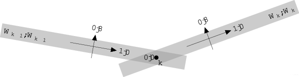
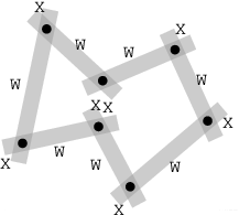
A polygon in superspace is specified through a sequence of vertices $X_{k}=(x_{k},\theta_{k},\bar{\theta}_{k})$ , $k=1,\ldots,n$ , see Fig. 1. For a null polygon we demand that the segment between two adjacent vertices is null, cf. Sec. 2.3,

x_{k,k+1}^{2}=0,\qquad x_{k,k+1}^{\scriptscriptstyle\mathrm{T}}\varepsilon\theta_{k,k+1}=0,\qquad\bar{\theta}_{k,k+1}\varepsilon x_{k,k+1}^{\scriptscriptstyle\mathrm{T}}=0.

(3.1)

The polygon is closed, hence we identify vertex $n+1$ with vertex $1$ , and more generally vertex numbers will be considered modulo $n$ .

Let us count the degrees of freedom of the polygon. Each vertex contributes $4|16$ degrees of freedom. The null condition for each segment amounts to $1|8$ constraints. In total, the polygon thus has $3n|8n$ degrees of freedom.

3.2 Spinor Variables

For the segment between vertices $k$ and $k+1$ of the polygon, we solve the null condition in terms of spinor helicity variables $\Lambda_{k}:=(\lambda_{k},\bar{\lambda}_{k},\eta_{k},\bar{\eta}_{k})$ , see Fig. 1 for the labelling of vertices and edges. The $\lambda$ ’s are 2-component bosonic vectors, the $\eta$ ’s are 4-component fermionic vectors. The general solution reads

x_{k,k+1}=\lambda_{k}\bar{\lambda}_{k},\qquad\theta_{k,k+1}=\lambda_{k}\eta_{k},\qquad\bar{\theta}_{k,k+1}=\bar{\eta}_{k}\bar{\lambda}_{k}.

(3.2)

Compatibility with the reality condition (2.5) implies the following complex conjugation properties

\lambda^{\dagger}_{k}=\pm\bar{\lambda}_{k},\qquad\eta^{\dagger}_{k}=\pm\bar{\eta}_{k},

(3.3)

with a common sign for both relations. The above parametrisation is invariant under the rescaling (reality conditions imply that $z$ is a pure complex phase)

\lambda_{k}\mapsto z_{k}\lambda_{k},\qquad\bar{\lambda}_{k}\mapsto z^{-1}_{k}\bar{\lambda}_{k},\qquad\eta_{k}\mapsto z^{-1}_{k}\eta_{k},\qquad\bar{\eta}_{k}\mapsto z_{k}\bar{\eta}_{k}.

(3.4)

Thus, we have $3|8$ degrees of freedom for each segment, but $4|16$ constraints for the closure of the polygon. In total there are $(3n-4)|(8n-16)$ degrees of freedom for the spinor variables. As the spinor variables are invariant under translations, a reference vertex provides the remaining $4|16$ degrees of freedom for the polygon.

Let us next derive the superconformal transformations of the spinor variables. As the intervals are translation-invariant, so are the spinor variables. For the superconformal boosts, we substitute the definition (3.2) into the boost transformation of the interval (2.14)

$\displaystyle\delta(\lambda_{k}\bar{\lambda}_{k})=$	$\displaystyle\ \lambda_{k}\bigl(-i(1-i\eta_{k}\bar{\eta}_{k})(\bar{\lambda}_{k}\varepsilon\rho\bar{\eta}_{k})\bar{\lambda}_{k}-2i\bar{\lambda}_{k}\varepsilon\rho\bar{\theta}_{k}\bigr)$
	$\displaystyle+\bigl(-i(1+i\eta_{k}\bar{\eta}_{k})(\eta_{k}\bar{\rho}\varepsilon\lambda_{k})\lambda_{k}-2i\theta_{k}\bar{\rho}\varepsilon\lambda_{k}\bigr)\bar{\lambda}_{k},$
$\displaystyle\delta(\lambda_{k}\eta_{k})=$	$\displaystyle\ \lambda_{k}\bigl((1+i\eta_{k}\bar{\eta}_{k})\bar{\lambda}_{k}+2i\eta_{k}\bar{\theta}_{k}\bigr)\varepsilon\rho$
	$\displaystyle-2i\lambda_{k}\eta_{k}\bar{\rho}\varepsilon\theta_{k}-2i\lambda_{k}\eta_{k}\bar{\rho}\varepsilon\lambda_{k}\eta_{k}-2i\theta_{k}\bar{\rho}\varepsilon\lambda_{k}\eta_{k},$
$\displaystyle\delta(\bar{\eta}_{k}\bar{\lambda}_{k})=$	$\displaystyle-2i\bar{\eta}_{k}\bar{\lambda}_{k}\varepsilon\rho\bar{\theta}_{k}-2i\bar{\theta}_{k}\varepsilon\rho\bar{\eta}_{k}\bar{\lambda}_{k}-2i\bar{\eta}_{k}\bar{\lambda}_{k}\varepsilon\rho\bar{\eta}_{k}\bar{\lambda}_{k}$
	$\displaystyle+\bar{\rho}\varepsilon\bigl(-(1-i\eta_{k}\bar{\eta}_{k})\lambda_{k}+2i\theta_{k}\bar{\eta}_{k}\bigr)\bar{\lambda}_{k}.$	(3.5)

These transformations can be split up into boost transformations for the spinor variables essentially because the null condition is superconformally invariant

$\displaystyle\delta\lambda_{k}=$	$\displaystyle+i\mathop{\mathrm{Tr}}(\rho\bar{\alpha}_{k}-\alpha_{k}\bar{\rho})\lambda_{k}-i(1+i\eta_{k}\bar{\eta}_{k})(\eta_{k}\bar{\rho}\varepsilon\lambda_{k})\lambda_{k}-2i\theta_{k}\bar{\rho}\varepsilon\lambda_{k},$
$\displaystyle\delta\bar{\lambda}_{k}=$	$\displaystyle-i\mathop{\mathrm{Tr}}(\rho\bar{\alpha}_{k}-\alpha_{k}\bar{\rho})\bar{\lambda}_{k}-i(1-i\eta_{k}\bar{\eta}_{k})(\bar{\lambda}_{k}\varepsilon\rho\bar{\eta}_{k})\bar{\lambda}_{k}-2i\bar{\lambda}_{k}\varepsilon\rho\bar{\theta}_{k},$
$\displaystyle\delta\eta_{k}=$	$\displaystyle-i\mathop{\mathrm{Tr}}(\rho\bar{\alpha}_{k}-\alpha_{k}\bar{\rho})\eta_{k}+(1+i\eta_{k}\bar{\eta}_{k})\bar{\lambda}_{k}\varepsilon\rho+2i\eta_{k}\bar{\theta}_{k}\varepsilon\rho$
	$\displaystyle-i(1-i\eta_{k}\bar{\eta}_{k})(\eta_{k}\bar{\rho}\varepsilon\lambda_{k})\eta_{k}-2i\eta_{k}\bar{\rho}\varepsilon\theta_{k},$
$\displaystyle\delta\bar{\eta}_{k}=$	$\displaystyle+i\mathop{\mathrm{Tr}}(\rho\bar{\alpha}_{k}-\alpha_{k}\bar{\rho})\bar{\eta}_{k}-i(1+i\eta_{k}\bar{\eta}_{k})(\bar{\lambda}_{k}\varepsilon\rho\bar{\eta}_{k})\bar{\eta}_{k}-2i\bar{\theta}_{k}\varepsilon\rho\bar{\eta}_{k}$
	$\displaystyle-(1-i\eta_{k}\bar{\eta}_{k})\bar{\rho}\varepsilon\lambda_{k}+2i\bar{\rho}\varepsilon\theta_{k}\bar{\eta}_{k}.$	(3.6)

Here the $\alpha$ ’s parametrise the transformation of the unphysical degree of freedom in (3.4).

3.3 Twistor Variables

The above boost transformations of the spinor variables (3.6) are somewhat intransparent. It is convenient to introduce so-called momentum twistor variables [24, 25] (cf. reviews in [26, 27]) to parametrise our null polygon. They will turn out to transform nicely. A momentum twistor $W_{k}$ and its conjugate $\bar{W}_{k}$ are complex projective $4|4$ vectors defined by

	$\displaystyle W_{k}$	$\displaystyle:=(-{\textstyle\frac{i}{2}}\lambda_{k}^{\scriptscriptstyle\mathrm{T}}\varepsilon,\mu_{k},\chi_{k}),$	$\displaystyle\mu_{k}$	$\displaystyle:=\lambda_{k}^{\scriptscriptstyle\mathrm{T}}\varepsilon x^{+}_{k},$	$\displaystyle\chi_{k}$	$\displaystyle:=\lambda_{k}^{\scriptscriptstyle\mathrm{T}}\varepsilon\theta_{k},$
	$\displaystyle\bar{W}_{k}$	$\displaystyle:=(\bar{\mu}_{k},-{\textstyle\frac{i}{2}}\varepsilon\bar{\lambda}_{k}^{\scriptscriptstyle\mathrm{T}},\bar{\chi}_{k}),$	$\displaystyle\bar{\mu}_{k}$	$\displaystyle:=-x^{-}_{k}\varepsilon\bar{\lambda}_{k}^{\scriptscriptstyle\mathrm{T}},$	$\displaystyle\bar{\chi}_{k}$	$\displaystyle:=-\bar{\theta}_{k}\varepsilon\bar{\lambda}_{k}^{\scriptscriptstyle\mathrm{T}}.$		(3.7)

Reality conditions for the twistors follow from (2.5,3.3). They impose the hermitian signature $(2,2|4)$ on $(W_{k},\bar{W}_{k})$ by means of a conjugation matrix $C$ written in $2,2,4$ block form¹¹ 1 The sign in the reality condition specifies an orientation of the corresponding polygon segment. The conjugation property can be fixed to $W_{k}^{\dagger}=C\bar{W}_{k}$ by rescaling the definition of $\bar{W}$ by $\pm 1$ .

W_{k}^{\dagger}=\pm C\bar{W}_{k},\qquad C=\left(\begin{array}[]{cc|c}0&1&0\\ 1&0&0\\ \hline\cr 0&0&1\end{array}\right).

(3.8)

As before, the superconformal transformations follow by substituting the definitions. For translations we obtain from (2.9) simply

$\displaystyle\delta\lambda_{k}^{\scriptscriptstyle\mathrm{T}}$	$\displaystyle=0,$	$\displaystyle\delta\bar{\lambda}_{k}^{\scriptscriptstyle\mathrm{T}}$	$\displaystyle=0,$
$\displaystyle\delta\chi_{k}$	$\displaystyle=\lambda_{k}^{\scriptscriptstyle\mathrm{T}}\varepsilon\psi,$	$\displaystyle\delta\bar{\chi}_{k}$	$\displaystyle=-\bar{\psi}\varepsilon\bar{\lambda}_{k}^{\scriptscriptstyle\mathrm{T}},$
$\displaystyle\delta\mu_{k}$	$\displaystyle=2i\chi_{k}\bar{\psi},$	$\displaystyle\delta\bar{\mu}_{k}$	$\displaystyle=-2i\psi\bar{\chi}_{k}.$	(3.9)

Boosts follow from (2.12,3.6)

$\displaystyle\delta\lambda_{k}^{\scriptscriptstyle\mathrm{T}}$	$\displaystyle=\beta_{k}\lambda_{k}^{\scriptscriptstyle\mathrm{T}}+2i\chi_{k}\bar{\rho},$	$\displaystyle\delta\bar{\lambda}_{k}^{\scriptscriptstyle\mathrm{T}}$	$\displaystyle=\bar{\beta}_{k}\bar{\lambda}_{k}^{\scriptscriptstyle\mathrm{T}}-2i\rho\bar{\chi}_{k},$
$\displaystyle\delta\chi_{k}$	$\displaystyle=\beta_{k}\chi_{k}+\mu_{k}\varepsilon\rho,$	$\displaystyle\delta\bar{\chi}_{k}$	$\displaystyle=\bar{\beta}_{k}\bar{\chi}_{k}-\bar{\rho}\varepsilon\bar{\mu}_{k},$
$\displaystyle\delta\mu_{k}$	$\displaystyle=\beta_{k}\mu_{k},$	$\displaystyle\delta\bar{\mu}_{k}$	$\displaystyle=\bar{\beta}_{k}\bar{\mu}_{k}.$	(3.10)

The $\beta$ ’s correspond to rescalings of the twistors $W_{k}$ and $\bar{W}_{k}$ . Due to the projective nature of twistors, the $\beta$ ’s are inessential, we can nevertheless state their expression in terms of spinor variables

	$\displaystyle\beta_{k}$	$\displaystyle:=+i\mathop{\mathrm{Tr}}(\rho\bar{\alpha}_{k}-\alpha_{k}\bar{\rho}-2\varepsilon\theta_{k}\bar{\rho})-i(1+i\eta_{k}\bar{\eta}_{k})(\eta_{k}\bar{\rho}\varepsilon\lambda_{k}),$
	$\displaystyle\bar{\beta}_{k}$	$\displaystyle:=-i\mathop{\mathrm{Tr}}(\rho\bar{\alpha}_{k}-\alpha_{k}\bar{\rho}+2\rho\bar{\theta}_{k}\varepsilon)-i(1-i\eta_{k}\bar{\eta}_{k})(\bar{\lambda}_{k}\varepsilon\rho\bar{\eta}_{k}).$		(3.11)

In summary, the twistors $W_{k}$ and $\bar{W}_{k}$ transform as projective fundamental and anti-fundamental representations of the superconformal algebra $\mathfrak{psu}(2,2|4)$ .

It is now straight-forward to construct the projective invariants

	$\displaystyle W_{j}\bar{W}_{k}$	$\displaystyle=-{\textstyle\frac{i}{2}}\lambda_{j}^{\scriptscriptstyle\mathrm{T}}\varepsilon\bar{\mu}_{k}-{\textstyle\frac{i}{2}}\mu_{j}\varepsilon\bar{\lambda}_{k}^{\scriptscriptstyle\mathrm{T}}+\chi_{j}\bar{\chi}_{k}$
		$\displaystyle={\textstyle\frac{i}{2}}\lambda_{j}^{\scriptscriptstyle\mathrm{T}}\varepsilon(x^{-}_{k}-x^{+}_{j}+2i\theta_{j}\bar{\theta}_{k})\varepsilon\bar{\lambda}_{k}^{\scriptscriptstyle\mathrm{T}}={\textstyle\frac{i}{2}}\lambda_{j}^{\scriptscriptstyle\mathrm{T}}\varepsilon x^{+-}_{j,k}\varepsilon\bar{\lambda}_{k}^{\scriptscriptstyle\mathrm{T}}.$		(3.12)

They transform as $\delta(W_{j}\bar{W}_{k})=(\beta_{j}+\bar{\beta}_{k})W_{j}\bar{W}_{k}$ . Proper invariants can be obtained as functions of these with vanishing weights in each of the twistors variables $W_{k}$ and, separately, their conjugates $\bar{W}_{k}$ .

Note that these momentum twistor variables are constrained. By virtue of (2.7) one finds

W_{k}\bar{W}_{k}=-{\textstyle\frac{i}{2}}\lambda_{k}^{\scriptscriptstyle\mathrm{T}}\varepsilon(x^{+}_{k}-x^{-}_{k}-2i\theta_{k}\bar{\theta}_{k})\varepsilon\bar{\lambda}_{k}^{\scriptscriptstyle\mathrm{T}}=0.

(3.13)

This means that the pair $W_{k},\bar{W}_{k}$ actually defines a (real) ambitwistor. Likewise one finds that contractions of adjacent twistors vanish

	$\displaystyle W_{k}\bar{W}_{k+1}$	$\displaystyle=+{\textstyle\frac{i}{2}}\lambda_{k}^{\scriptscriptstyle\mathrm{T}}\varepsilon\lambda_{k}(1-i\eta_{k}\bar{\eta}_{k})\bar{\lambda}_{k}\varepsilon\bar{\lambda}_{k+1}^{\scriptscriptstyle\mathrm{T}}=0,$
	$\displaystyle W_{k+1}\bar{W}_{k}$	$\displaystyle=-{\textstyle\frac{i}{2}}\lambda_{k+1}^{\scriptscriptstyle\mathrm{T}}\varepsilon\lambda_{k}(1+i\eta_{k}\bar{\eta}_{k})\bar{\lambda}_{k}\varepsilon\bar{\lambda}_{k}^{\scriptscriptstyle\mathrm{T}}=0.$		(3.14)

We shall refer to a sequence $W_{k},\bar{W}_{k}$ , $k=1,\ldots,n$ , subject to the constraints

W_{j}\bar{W}_{k}=0\quad\text{for}\quad|j-k|\leq 1

(3.15)

as momentum ambitwistors [24, 25].

We can now count the real degrees of freedom of the twistor variables. Both $W_{k}$ and $\bar{W}_{k}$ contribute $4|4$ degrees of freedom. Independent rescalings of $W_{k}$ and $\bar{W}_{k}$ eliminate two degrees of freedom, and the ambitwistor condition a third one. Each ambitwistor thus has $5|8$ degrees of freedom. There are two additional constraints for each pair of adjacent vertices, leaving $3n|8n$ degrees of freedom. This matches precisely the previous counting for the null polygon. It shows that a null polygon in superspace is described by a sequence a momentum ambitwistors.

3.4 Comparison

We have discussed three different formulations for null polygons in superspace:

•

The first one specifies the vertices $X_{k}=(x_{k},\theta_{k},\bar{\theta}_{k})$ . Two adjacent vertices are constrained to be null-separated.
•

The second formulation specifies the segments in terms of spinor variables $\Lambda_{k}=(\lambda_{k},\bar{\lambda}_{k},\eta_{k},\bar{\eta}_{k})$ . The null conditions are automatically satisfied, but constraints are needed to guarantee closure of the polygon. This formulation is invariant under translations, a reference vertex is needed to locate the polygon in superspace.
•

A final description uses momentum ambitwistors $(W_{k},\bar{W}_{K})$ to describe the segments and vertices. Three constraints per segment are needed to guarantee that the segments intersect properly.

In all cases, the polygon is described by $3n|8n$ degrees of freedom, and we displayed their relations explicitly.

Let us compare this to the case of null polygons in chiral superspace which has $4|8$ coordinates only (the anti-chiral case is equivalent). The above discussion fully applies through projection of the full superspace $(x,\theta,\bar{\theta})$ onto the chiral subspace $(x^{+},\theta)$ ; in effect, one disregards all $\bar{\theta}$ ’s, $\bar{\eta}$ ’s and $\bar{W}$ ’s. The chiral null polygon is then described by $3n|4n$ degrees of freedom. There is, however, one noteworthy difference: When discarding the $\bar{W}$ ’s, all constraints on chiral momentum twistors drop out. Unconstrained chiral momentum twistors provide all the necessary $3n|4n$ degrees of freedom of the polygon! This crucial benefit comes along with the minor shortcoming that chiral superspace requires either $(2,2)$ split signature or complexified Minkowski space. If reality conditions for $(3,1)$ signature are imposed on chiral momentum twistors, one indeed recovers the conjugate twistors along with the constraints.

Finally, we compare these two cases to the purely bosonic case by disregarding all fermionic components. The bosonic null polygon is described by $3n$ degrees of freedom. The formulation in terms of momentum twistors is equivalent to the formulation in terms of momentum ambitwistors. The two are related by the identification $\bar{W}_{k,A}=\varepsilon_{ABCD}W_{k-1}^{B}W_{k}^{C}W_{k+1}^{D}$ up to an inessential factor. It automatically implies the momentum ambitwistor constraints (3.15). Unfortunately, in the supersymmetric case, the tensor $\varepsilon_{ABCD}$ is not invariant, and a supersymmetrisation does not exist. Hence, we are forced to use the ambitwistor formulation for the full superspace.

4 Fat Null Polygons

Next we wish to define the null polygon curve. Here we encounter an interesting surprise.

4.1 Thin Segments

So far we have merely defined the vertices. Two adjacent vertices $k$ and $k+1$ are null-separated, and we shall connect them by a null curve. The obvious choice is

$\displaystyle x(\tau)$	$\displaystyle=x_{k}+(\lambda_{k}\bar{\lambda}_{k}+i\lambda_{k}\eta_{k}\bar{\theta}_{k}-i\theta_{k}\bar{\eta}_{k}\bar{\lambda}_{k})\tau,$
$\displaystyle\theta(\tau)$	$\displaystyle=\theta_{k}+\lambda_{k}\eta_{k}\tau,$
$\displaystyle\bar{\theta}(\tau)$	$\displaystyle=\bar{\theta}_{k}+\bar{\eta}_{k}\bar{\lambda}_{k}\tau.$	(4.1)

Unfortunately, it turns out that this kind of curve is not stable under a superconformal boost transformation: In the above curve all coordinates are linear in $\tau$ . After the transformation, the coordinates are not linear. In the bosonic case, a compensating reparametrisation $\tau\to\tau^{\prime}$ is required to recover linearity. In the extended supersymmetric case, such a reparametrisation does not exist in general. To see this, let us consider $\theta(\tau)$ . The second derivative $\ddot{\theta}$ originally vanishes. For the boost (2.12) of the curve we find

\frac{d^{2}\delta\theta}{d\tau^{2}}=2i(\eta_{k}\bar{\eta}_{k})\lambda_{k}\bar{\lambda}_{k}\varepsilon\rho-4i(\eta_{k}\bar{\rho}\varepsilon\lambda_{k})\lambda_{k}\eta_{k}\stackrel{{\scriptstyle?}}{{=}}\frac{d^{2}\delta\tau}{d\tau^{2}}\,\dot{\theta}.

(4.2)

The identity on the right hand side is the condition for linearity up to reparametrisation of $\tau$ . The second term in the middle is indeed of the desired form with $d^{2}\delta\tau/d\tau^{2}=-4i(\eta_{k}\bar{\rho}\varepsilon\lambda_{k})$ because $\dot{\theta}=\lambda_{k}\eta_{k}$ . The first term in the middle, however, is not. It would require $\rho$ to be collinear to $\eta_{k}$ which generically does not hold, certainly not for all polygon segments. In conclusion, boost transformations map polygons constructed from naive straight null segments (4.1) to some other shape, cf. Fig. 2. Furthermore, we did not find a suitable alternative definition for straight null curves which has this stability property. This may seem unfortunate because Wilson loops on such null polygons would appear not to transform nicely, and we could not make use of superconformal symmetry. As we shall see shortly, this in fact does not pose a problem.

4.2 Fat Null Lines

There is an alternative characterisation of straight null lines in bosonic spacetime which we can use for superspace as well: Consider two fixed points $x_{0}$ and $x_{1}$ which are null-separated. A straight null line passing through $x_{0}$ and $x_{1}$ is the set of all points $x$ which are null-separated from both $x_{0}$ and $x_{1}$ . This defines a straight line because any three null vectors $x-x_{0}$ , $x_{1}-x$ and $x_{0}-x_{1}$ in Minkowski space which add up to zero are necessarily collinear. This definition is manifestly conformal because the null condition is. Moreover it carries over to superspace straight-forwardly.

Consider therefore two null-separated points $X_{0}$ and $X_{1}$ in superspace. According to (3.2) we can write the superspace interval (2.13) as $x_{0,1}=\lambda\bar{\lambda}$ , $\theta_{0,1}=\lambda\eta$ , $\bar{\theta}_{0,1}=\bar{\eta}\bar{\lambda}$ . This provides us with a parametrisation of $X_{1}$ in terms of $X_{0}$ and the spinors $\lambda,\bar{\lambda},\eta,\bar{\eta}$

x_{1}=x_{0}+\lambda\bar{\lambda}+i\lambda\eta\bar{\theta}_{0}-i\theta_{0}\bar{\eta}\bar{\lambda},\qquad\theta_{1}=\theta_{0}+\lambda\eta,\qquad\bar{\theta}_{1}=\bar{\theta}_{0}+\bar{\eta}\bar{\lambda}.

(4.3)

All points $X$ at null-separation to $X_{0}$ must therefore be of the same form but with different $\lambda^{\prime},\bar{\lambda}^{\prime},\eta^{\prime},\bar{\eta}^{\prime}$ . Null-separation from $X_{1}$ then merely forces $\lambda^{\prime}\sim\lambda$ and $\bar{\lambda}^{\prime}\sim\bar{\lambda}$ . Hence we can write the most general solution as

x=x_{0}+\tau\lambda\bar{\lambda}+i\lambda\sigma\bar{\theta}_{0}-i\theta_{0}\bar{\sigma}\bar{\lambda},\qquad\theta=\theta_{0}+\lambda\sigma,\qquad\bar{\theta}=\bar{\theta}_{0}+\bar{\sigma}\bar{\lambda}.

(4.4)

The solution $X(\tau,\sigma,\bar{\sigma})$ is parametrised explicitly through one bosonic coordinate $\tau$ and a pair of complex conjugate 4-component fermionic coordinates $(\sigma,\bar{\sigma})$ . Curiously, the null line in superspace is “fattened” by $8$ fermionic coordinates, see Fig. 3, cf. [28, 29, 30].²² 2 The fattening (by 4 fermionic coordinates) also applies to null polygons in chiral superspace.

The fatness of the null line explains our difficulty in finding a proper straight line between two null-separated vertices. With regard to superconformal transformations, a fat null line is a very natural object, its shape manifestly remains stable. Conversely, there appears to be no distinguished submanifold of dimension $1|0$ . Our attempt (4.1) to set $\sigma=\eta\tau$ and $\bar{\sigma}=\bar{\eta}\tau$ is one possibility, but there is nothing that prevents conformal transformations from distorting our choice. In Sec. 5 we shall explain that all curves on a fat null line are physically equivalent. In other words, a fat null line actually defines a physically unique curve.

4.3 Ambitwistors

Before we continue with the physical implication of fat lines, let us return to the insight that null polygons are specified by a sequence of ambitwistors, and let us take it seriously (see [26, 27] for reviews of twistors and ref. [31] for an in-depth discussion of the relevant twistor space geometry).

A twistor $W=(-{\textstyle\frac{i}{2}}\lambda^{\scriptscriptstyle\mathrm{T}}\varepsilon,\mu,\chi)$ describes a null subspace of superspace through the equations for the chiral coordinates $(x^{+},\theta)$

\lambda^{\scriptscriptstyle\mathrm{T}}\varepsilon x^{+}=\mu,\qquad\lambda^{\scriptscriptstyle\mathrm{T}}\varepsilon\theta=\chi.

(4.5)

These $2|4$ equations constrain as many coordinates of (complexified) superspace. Embedding the twistor into chiral superspace, the dimension is $2|4$ . We can parametrise the solution explicitly through a 2-component bosonic vector $\bar{\kappa}$ and a 4-component fermionic vector $\sigma$

x^{+}(\bar{\kappa},\sigma)=x^{+}_{0}+\lambda\bar{\kappa},\qquad\theta(\bar{\kappa},\sigma)=\theta_{0}+\lambda\sigma.

(4.6)

Here $x^{+}_{0},\theta_{0}$ are particular solutions of the inhomogeneous equations. In full superspace, the anti-chiral coordinates $\bar{\theta}$ are unconstrained, and hence the dimension of the twistor in full superspace is $2|12$ .

A conjugate twistor $\bar{W}$ describes an analogous subspace

-x^{-}\varepsilon\bar{\lambda}^{\scriptscriptstyle\mathrm{T}}=\bar{\mu},\qquad-\bar{\theta}\varepsilon\bar{\lambda}^{\scriptscriptstyle\mathrm{T}}=\bar{\chi}.

(4.7)

Superficially, the intersection of the subspaces given by $W$ and $\bar{W}$ is a space of codimension $4|8$ , i.e. of dimension $0|8$ . This simple consideration misses the fact that the two twistor equations are generally incompatible because of the relation (2.7) between $x^{+}$ and $x^{-}$ . Compatibility requires the ambitwistor condition $W\bar{W}=0$ :

0=\lambda^{\scriptscriptstyle\mathrm{T}}\varepsilon(x^{+}-x^{-}-2i\theta\bar{\theta})\varepsilon\bar{\lambda}^{\scriptscriptstyle\mathrm{T}}=\mu\varepsilon\bar{\lambda}^{\scriptscriptstyle\mathrm{T}}+\lambda^{\scriptscriptstyle\mathrm{T}}\varepsilon\bar{\mu}+2i\chi\bar{\chi}=2iW\bar{W}.

(4.8)

The resulting intersection is thus bigger by one bosonic dimension, namely it has dimension $1|8$ , see Fig. 4 for an illustration of the twistors and their intersection. Note that the intersection is contained in real superspace. It is given precisely by the above explicit parametrisation of the fat null line in (4.4). Note that the chiral coordinates $x^{\pm}$ both take the predicted form (4.6) for chiral twistors for a suitable choice of $\bar{\kappa},\kappa$

x^{+}=x^{+}_{0}+\lambda(\tau\bar{\lambda}+i\sigma\bar{\sigma}\bar{\lambda}+2i\sigma\bar{\theta}_{0}),\qquad x^{-}=x^{-}_{0}+(\tau\lambda-i\sigma\bar{\sigma}\lambda-2i\theta_{0}\bar{\sigma})\bar{\lambda}.

(4.9)

Bosonically, an ambitwistor describes a null line. In superspace, however, the null line is fattened by 8 real fermionic coordinates, see Fig. 3. Under superconformal transformations the ambitwistor $(W,\bar{W})$ transforms as a complex conjugate pair of projective fundamental representations. The corresponding fat null line transforms accordingly.

We have seen above that a null polygon in superspace can be given in terms of a sequence of ambitwistors $(W_{k},\bar{W}_{k})$ . Taken at face value, our polygon can be viewed as a sequence of fat null lines. The additional conditions

W_{k-1}\bar{W}_{k}=W_{k}\bar{W}_{k-1}=0

(4.10)

ensure that two consecutive fat segments intersect. Although they are fat, they generically intersect in a (thin) point of dimension $0|0$ , namely the vertex $X_{k}=(x_{k},\theta_{k},\bar{\theta}_{k})$ , see Fig. 5. This is how the vertices are specified by a sequence of ambitwistors. Let us also remark that there is a unique ambitwistor which connects two null-separated points, see Fig. 6. This is how the ambitwistors are specified by a sequence of vertices.

4.4 Dual Polygon in Ambitwistor Space

A null polygon consists of a sequence of vertices and edges. The vertices are points $X_{k}=(x_{k},\theta_{k},\bar{\theta}_{k})$ in $\mathcal{N}=4$ Minkowski superspace $\mathbb{M}=\mathbb{R}^{3,1}\times\mathbb{C}^{0|8}=\mathbb{R}^{3,1|16}$ . As described above, the edges are fat null lines in $\mathbb{M}$ . Alternatively, the edges can be specified through a sequence of ambitwistors $(W_{k},\bar{W}_{k})$ . Now we can also view an ambitwistor as a point in ambitwistor space $\mathbb{Q}$ . When the latter points are connected by edges, we obtain a dual polygon in ambitwistor space [26]. Let us briefly discuss the nature of this dual polygon.

We specify an ambitwistor $(W,\bar{W})$ through a twistor $W\in\mathbb{C}^{2,2|4}\backslash\{0\}$ and its complex conjugate $\bar{W}$ , which is hence not an independent quantity.³³ 3 Very often in discussions of twistor space, the corresponding Minkowski space is assumed to have complex or $(2,2)$ split signature. For our purposes there is no need to deviate from real $(3,1)$ signature in what follows. To translate the discussion to complex signature one would complexify real spaces and double complex spaces, e.g. $\mathbb{R}^{3,1}\mapsto\mathbb{C}^{4}$ and $\mathbb{C}\mathbb{P}^{1,2}\mapsto\mathbb{C}\mathbb{P}^{3}\times\mathbb{C}\mathbb{P}^{3}$ . To translate to split signature instead, one chooses a different real form for the complexified spaces, e.g. $\mathbb{R}^{3,1}\mapsto\mathbb{R}^{2,2}$ and $\mathbb{C}\mathbb{P}^{1,2}\mapsto\mathbb{R}\mathbb{P}^{3}\times\mathbb{R}\mathbb{P}^{3}$ . Ambitwistors are projectively identified, i.e. $(W,\bar{W})\simeq(zW,\bar{z}\bar{W})$ for any $z\in\mathbb{C}^{*}$ . Moreover, they satisfy the condition $W\bar{W}=0$ . Altogether this defines a $5|8$ -dimensional real subspace $\mathbb{Q}$ of the complex projective identification of $\mathbb{C}^{2,2|4}\backslash\{0\}$ , see Fig. 7. The space $\mathbb{Q}$ will be called (real) ambitwistor space (in the twistor space literature it is usually called the space of projective null twistors $\mathbb{PN}$ ).

Consider now the situation at a vertex of the polygon in $\mathbb{M}$ . It is described by two fat null lines which meet in a point. They correspond to two ambitwistors $(W,\bar{W})$ and $(W^{\prime},\bar{W}^{\prime})$ which obey the additional condition $W\bar{W}^{\prime}=W^{\prime}\bar{W}=0$ that makes the associated lines intersect. The latter condition implies that all the points on the $\mathbb{C}\mathbb{P}^{1}$ joining $(W,\bar{W})$ and $(W^{\prime},\bar{W}^{\prime})$

(zW+z^{\prime}W^{\prime},\bar{z}\bar{W}+\bar{z}^{\prime}\bar{W}^{\prime})\quad\mbox{for all }z,z^{\prime}\in\mathbb{C}

(4.11)

are also ambitwistors because they satisfy

(zW+z^{\prime}W^{\prime})(\bar{z}\bar{W}+\bar{z}^{\prime}\bar{W}^{\prime})=z\bar{z}W\bar{W}+z\bar{z}^{\prime}W\bar{W}^{\prime}+z^{\prime}\bar{z}W^{\prime}\bar{W}+z^{\prime}\bar{z}^{\prime}W^{\prime}\bar{W}^{\prime}=0.

(4.12)

In other words, the points $W$ and $W^{\prime}$ are connected by a $\mathbb{C}\mathbb{P}^{1}$ which resides entirely within ambitwistor space $\mathbb{Q}$ .⁴⁴ 4 We thank David Skinner for pointing out this interpretation. Hence, the dual of two intersecting lines in $\mathbb{M}$ are two points in $\mathbb{Q}$ joined by a $\mathbb{C}\mathbb{P}^{1}$ inside $\mathbb{Q}$ .

We conclude that the dual of a null polygon in $\mathbb{M}$ is a polygon in $\mathbb{Q}$ whose edges are $\mathbb{C}\mathbb{P}^{1}$ ’s, see Fig. 8. Incidentally the edges of the dual polygon are $2|0$ -dimensional, i.e. they are also fat, moreover along bosonic directions. In fact, this duality is one-to-one because a $\mathbb{C}\mathbb{P}^{1}$ in $\mathbb{Q}$ also describes precisely a single point in $\mathbb{M}$ : A $\mathbb{C}\mathbb{P}^{1}$ can be specified by two points $W,W^{\prime}\in\mathbb{C}^{2,2|4}\backslash\{0\}$ which amounts to $16|16$ real degrees of freedom. They must satisfy the 4 real constraints $W\bar{W}=W\bar{W}^{\prime}=W^{\prime}\bar{W}=W^{\prime}\bar{W}^{\prime}=0$ . Furthermore, any pair of complex linear combinations of $W$ and $W^{\prime}$ describes the same $\mathbb{C}\mathbb{P}^{1}$ which removes another 8 real degrees of freedom. Hence, the embedding of a $\mathbb{C}\mathbb{P}^{1}$ into $\mathbb{Q}$ has $4|16$ moduli which represents a point in $\mathbb{M}$ . Geometrically, the $\mathbb{C}\mathbb{P}^{1}$ is the sphere which describes the set of all null directions around a point.

Finally, let us daydream about a combination $\mathbb{M}\mathbb{Q}$ of Minkowski space $\mathbb{M}$ and ambitwistor space $\mathbb{Q}$ which may have some use. The points of this space describe points in $\mathbb{M}$ along with a null line that passes through the point. Alternatively, it is a point in $\mathbb{Q}$ along with a $\mathbb{C}\mathbb{P}^{1}$ in $\mathbb{Q}$ that passes through the point. Both of these interpretations lead to a dimension of $6|16=(4|16)+(2|0)=(5|8)+(1|8)$ . The space $\mathbb{M}\mathbb{Q}$ can be called the space of null rays in $\mathbb{M}$ , i.e. points together with a null direction. Technically, a point in $\mathbb{M}\mathbb{Q}$ is given by a point $X=(x,\theta,\bar{\theta})\in\mathbb{M}$ and an ambitwistor $(W,\bar{W})\in\mathbb{Q}$ subject to the conditions specified in (4.5,4.7).

A null polygon can be mapped to this space as a polygon with twice as many vertices and edges. The vertices in $\mathbb{M}\mathbb{Q}$ correspond to the rays at the beginning and end of each of the edges. The edges connect the points along fibres of $\mathbb{M}$ and $\mathbb{Q}$ in an alternating fashion, see Fig. 9. The nice feature of this representation is that it includes both the spacetime polygon and the twistor polygon as projections onto the spaces $\mathbb{M}$ and $\mathbb{Q}$ , respectively.

Finally, we can note that the complexifications of the above spaces have representations as various flag manifolds of $\mathbb{C}^{4|4}$ , see e.g. [31, 32].⁵⁵ 5 We thank David Mesterhazy and David Skinner for discussions. Chiral twistor space $\mathbb{C}\mathbb{P}^{3|4}$ equals the flag manifold $\mathbb{F}_{1|0}$ while anti-chiral twistor space equals the dual flag manifold $\mathbb{F}_{3|4}$ . Chiral superspace corresponds to $\mathbb{F}_{2|0}$ while antichiral superspace is the dual $\mathbb{F}_{2|4}$ . Combinations of these flags yield the above spaces in an obvious fashion: Ambitwistor space is a combination of the two chiral twistor spaces $\mathbb{Q}=\mathbb{F}_{1|0;3|4}$ . Full superspace is a combination of the two chiral superspaces $\mathbb{M}=\mathbb{F}_{2|0;2|4}$ . The space of null rays is $\mathbb{M}\mathbb{Q}=\mathbb{F}_{1|0;2|0;2|4;3|4}$ . The latter three spaces are self-dual and they have real slices corresponding to Minkowski signature.

5 Curves on Fat Null Lines

In this section we will review the physical equivalence of all curves on a fat null line for the cases of the trajectory of the $\mathcal{N}=4$ supersymmetric particle and for Wilson lines in $\mathcal{N}=4$ supersymmetric Yang–Mills theory.

5.1 The Superparticle and $\kappa$ -Symmetry

Physically, we can think of a Wilson loop as the phase picked up by a non-dynamical charged particle moving in its own gauge field. In the case of super-Wilson loops, the same holds but this time we have to consider the motion of a superparticle in superspace. The superparticle in full superspace has a fermionic gauge symmetry called $\kappa$ -symmetry [33].

As noticed in ref. [34], for $\mathcal{N}=1$ super-Yang-Mills in ten dimensions, the translations in the fermionic directions of the fat lines are $\kappa$ -symmetry transformations. Here we redo a similar analysis for $\mathcal{N}=4$ super-Yang-Mills in four dimensions. This could be done by dimensionally reducing the $D=10$ , $\mathcal{N}=1$ analysis, but we will redo it from scratch instead.

Let us now write down the worldline superparticle action with $\mathcal{N}=4$ supersymmetry. According to (2.13) the supercovariant momentum reads

\pi=\dot{x}+i\theta\dot{\bar{\theta}}-i\dot{\theta}\bar{\theta}.

(5.1)

Then, the worldline superparticle action is ( $g$ is the worldline einbein)

S={\textstyle\frac{1}{2}}\int d\tau\,g\,\pi^{2}.

(5.2)

This action is manifestly superconformal invariant since the momentum squared transforms homogeneously under inversions, by a factor which can be absorbed by the einbein $g$ .

It is easy to show that the constraints in eq. (2.15) follow from the equations of motion of the action (5.2) and that the solution in (4.4) is the general solution of these equations of motion.

The worldline reparametrisations are gauge symmetries which can be fixed by setting $g$ to be constant (but this gauge condition is not preserved by superconformal transformations).

Now we can explain in a different way why a straight light-like line in full superspace is not preserved by superconformal transformations. In the language of eq. (4.4), if we take $\sigma$ and $\bar{\sigma}$ to be linear in $\tau$ , after a superconformal transformation we need need to perform a compensating worldline reparametrisation $\tau\to\tau^{\prime}(\tau)$ to preserve the gauge $g=\text{const}$ . Since this reparametrisation is not linear in $\tau$ , the odd coordinates $\sigma$ and $\bar{\sigma}$ will not be linear in the new worldline coordinate $\tau^{\prime}$ .

The action in eq. (5.2) is also invariant under a local $\kappa$ -symmetry which acts as

\delta\theta=\pi\bar{\kappa},\quad\delta\bar{\theta}=\kappa\pi,\quad\delta x=-i\theta\kappa\pi+i\pi\kappa\bar{\theta},\quad\delta g=-2ig\mathop{\mathrm{Tr}}\bigl(\bar{\kappa}\dot{\bar{\theta}}-\dot{\theta}\kappa\bigr).

(5.3)

Now, we act with $\kappa$ -symmetry on a superparticle at the point $(x,\theta,\bar{\theta})$ whose supermomentum $\pi$ is light-like, i.e. $\pi=\lambda\bar{\lambda}$ . We obtain

\delta x=i\lambda\sigma\bar{\theta}-i\theta\bar{\sigma}\bar{\lambda},\qquad\delta\theta=\lambda\sigma,\qquad\delta\bar{\theta}=\bar{\sigma}\bar{\lambda},

(5.4)

where we introduced the abbreviations $\sigma=\bar{\lambda}\bar{\kappa}$ , $\bar{\sigma}=\kappa\lambda$ . Comparison to (4.4) shows that $\kappa$ -symmetry can shift the point along any of the fermionic directions of a fat null line. This implies that all paths along this fat null line should be considered physically equivalent because $\kappa$ -symmetry is a gauge symmetry, cf. Fig. 10.

So we see that the $\kappa$ -symmetry transformations generate a $(0\lvert 8)$ -dimensional space (the quantities $\sigma$ and $\bar{\sigma}$ are complex conjugate fermionic coordinates with four complex dimensions, or eight real dimensions). Here we notice a reduction by half of the number of transformation parameters; we started with 16 real degrees of freedom in $\kappa$ and $\bar{\kappa}$ , but the latter only appear in the combinations $\sigma$ and $\bar{\sigma}$ , in which half of the degrees of freedom were projected out.

Using the $\kappa$ -symmetry transformations in eq. (5.4), we can compute its action on the twistor variables defined in eqs. (4.5,4.7). It is very easy to see that the twistor variables are invariant under $\kappa$ symmetry transformations. This was first noticed in ref. [35].

5.2 Yang–Mills Connection

Next we will discuss the implications of the fatness of null lines for Wilson lines in $\mathcal{N}=4$ SYM [36, 37]. As a first step we will review the $\mathcal{N}=4$ superspace formulation [38], in the next section we will apply it to Wilson lines.

To define Yang–Mills theory, we introduce a gauge connection one-form $A$ on superspace. A generic gauge connection would have way too many degrees of freedom as compared to the fields of $\mathcal{N}=4$ supersymmetric Yang–Mills theory. Therefore one must impose constraints on $A$ which is achieved by forcing some components of the associated field strength $F=dA+A^{2}$ to zero. This in turn not only reduces to the desired field content, but also enforces the equations of motion.

Before we continue, let us briefly discuss differential forms on superspace. It is convenient to express the components of differential forms in terms of the superspace vielbein $(d\theta^{\beta a},d\bar{\theta}_{b}{}^{\dot{\alpha}},e^{\beta\dot{\alpha}})$ where, according to (2.13),⁶⁶ 6 The differential operator $d$ obeys the same statistics as fermions. Consequently, $d\theta$ is bosonic.

e=dx-id\theta\bar{\theta}-i\theta d\bar{\theta}.

(5.5)

In particular, the exterior derivative $d$ can be expanded in this basis

d:=d\theta^{\beta a}\frac{\partial}{\partial\theta^{\beta a}}+d\bar{\theta}_{b}{}^{\dot{\alpha}}\frac{\partial}{\partial\bar{\theta}_{b}{}^{\dot{\alpha}}}+dx^{\beta\dot{\alpha}}\frac{\partial}{\partial x^{\beta\dot{\alpha}}}=d\theta^{\beta a}D_{a\beta}-d\bar{\theta}_{b}{}^{\dot{\alpha}}\bar{D}_{\dot{\alpha}}{}^{b}+e^{\beta\dot{\alpha}}\partial_{\dot{\alpha}\beta}.

(5.6)

Comparison of the definition of $d$ gives rise to supersymmetry covariant derivatives

D_{a\beta}=\frac{\partial}{\partial\theta^{\beta a}}+i\bar{\theta}_{a}{}^{\dot{\gamma}}\frac{\partial}{\partial x^{\beta\dot{\gamma}}}\,,\qquad\bar{D}_{\dot{\alpha}}{}^{b}=-\frac{\partial}{\partial\bar{\theta}_{b}{}^{\dot{\alpha}}}-i\theta^{a\gamma}\frac{\partial}{\partial x^{\gamma\dot{\alpha}}}\,,\qquad\partial_{\dot{\alpha}\beta}=\frac{\partial}{\partial x^{\beta\dot{\alpha}}}\,.

(5.7)

which satisfy the $\mathcal{N}=4$ super-Poincaré algebra with a flipped sign

\big\{D_{a\beta},D_{c\delta}\big\}=\big\{\bar{D}_{\dot{\alpha}}{}^{b},\bar{D}_{\dot{\gamma}}{}^{d}\big\}=0,\qquad\big\{D_{a\beta},\bar{D}_{\dot{\gamma}}{}^{d}\big\}=-2i\delta_{a}^{d}\partial_{\dot{\gamma}\beta}.

(5.8)

The expansions of a generic gauge connection $A$ and its associated field strength $F=dA+A^{2}$ read

$\displaystyle A=\mathord{}$	$\displaystyle d\theta^{\beta a}A_{a\beta}-d\bar{\theta}_{b}{}^{\dot{\alpha}}\bar{A}_{\dot{\alpha}}{}^{b}+e^{\beta\dot{\alpha}}A_{\dot{\alpha}\beta},$
$\displaystyle F=\mathord{}$	$\displaystyle{\textstyle\frac{1}{2}}d\theta^{\beta a}d\theta^{\delta c}F_{a\beta c\delta}+{\textstyle\frac{1}{2}}d\bar{\theta}_{b}{}^{\dot{\alpha}}d\bar{\theta}_{d}{}^{\dot{\gamma}}\bar{F}_{\dot{\alpha}}{}^{b}{}_{\dot{\gamma}}{}^{d}-d\theta^{\beta a}d\bar{\theta}_{d}{}^{\dot{\gamma}}F_{a\beta\dot{\gamma}}{}^{d}$
	$\displaystyle-d\theta^{\beta a}e^{\delta\dot{\gamma}}F_{a\beta\dot{\gamma}\delta}-e^{\beta\dot{\alpha}}d\bar{\theta}_{d}{}^{\dot{\gamma}}\bar{F}_{\dot{\alpha}\beta\dot{\gamma}}{}^{d}+{\textstyle\frac{1}{2}}e^{\beta\dot{\alpha}}e^{\delta\dot{\gamma}}F_{\dot{\alpha}\beta\dot{\gamma}\delta}.$	(5.9)

We use the connection to define a gauge covariant derivative $\mathcal{D}=d+A$ , or in components

\mathcal{D}_{a\beta}=D_{a\beta}+A_{a\beta},\qquad\bar{\mathcal{D}}_{\dot{\alpha}}{}^{b}=\bar{D}_{\dot{\alpha}}{}^{b}+\bar{A}_{\dot{\alpha}}{}^{b},\qquad\mathcal{D}_{\dot{\alpha}\beta}=\partial_{\dot{\alpha}\beta}+A_{\dot{\alpha}\beta}.

(5.10)

The components of the gauge-covariant field strength read

	$\displaystyle F_{a\beta c\delta}$	$\displaystyle=\big\{\mathcal{D}_{a\beta},\mathcal{D}_{c\delta}\big\},$	$\displaystyle\bar{F}_{\dot{\alpha}}{}^{b}{}_{\dot{\gamma}}{}^{d}$	$\displaystyle=\big\{\bar{\mathcal{D}}_{\dot{\alpha}}{}^{b},\bar{\mathcal{D}}_{\dot{\gamma}}{}^{d}\big\},$	$\displaystyle F_{a\beta\dot{\gamma}}{}^{d}$	$\displaystyle=\big\{\mathcal{D}_{a\beta},\bar{\mathcal{D}}_{\dot{\gamma}}{}^{d}\big\}+2i\delta_{a}^{d}\mathcal{D}_{\beta\dot{\gamma}},$
	$\displaystyle F_{a\beta\dot{\gamma}\delta}$	$\displaystyle=\big[\mathcal{D}_{a\beta},\mathcal{D}_{\dot{\gamma}\delta}\big],$	$\displaystyle\bar{F}_{\dot{\alpha}\beta\dot{\gamma}}{}^{d}$	$\displaystyle=\big[\mathcal{D}_{\dot{\alpha}\beta},\bar{\mathcal{D}}_{\dot{\gamma}}{}^{d}\big],$	$\displaystyle F_{\dot{\alpha}\beta\dot{\gamma}\delta}$	$\displaystyle=\big[\mathcal{D}_{\dot{\alpha}\beta},\mathcal{D}_{\dot{\gamma}\delta}\big].$		(5.11)

The constraint to reduce the connection $A$ to the field content of $\mathcal{N}=4$ SYM is imposed via the lowest components of the field strength $F$

F_{a\beta c\delta}=\varepsilon_{\beta\delta}\bar{\Phi}_{ac},\qquad\bar{F}_{\dot{\alpha}}{}^{b}{}_{\dot{\gamma}}{}^{d}=\varepsilon_{\dot{\alpha}\dot{\gamma}}\Phi^{bd},\qquad F_{a\beta\dot{\gamma}}{}^{d}=0,\qquad\Phi^{ab}={\textstyle\frac{1}{2}}e^{i\alpha}\varepsilon^{abcd}\bar{\Phi}_{cd}.

(5.12)

Here the expansion of superfields $\Phi$ and $\bar{\Phi}$ in terms of fermionic coordinates contains the scalars of $\mathcal{N}=4$ SYM as lowest components. The phase $\alpha$ in the relation between $\Phi$ and $\bar{\Phi}$ has no physical significance and we can safely set it to zero. The Bianchi identities $dF+FA+AF=0$ then fix all the remaining higher components of $F$ , in particular

F_{a\beta\dot{\gamma}\delta}=\varepsilon_{\beta\delta}\bar{\Psi}_{a\dot{\gamma}},\qquad\bar{F}_{\dot{\alpha}\beta\dot{\gamma}}{}^{d}=\varepsilon_{\dot{\alpha}\dot{\gamma}}\Psi_{\beta}{}^{d},\qquad F_{\dot{\alpha}\beta\dot{\gamma}\delta}=\varepsilon_{\beta\delta}\bar{\Gamma}_{\dot{\alpha}\dot{\gamma}}+\varepsilon_{\dot{\alpha}\dot{\gamma}}\Gamma_{\beta\delta},

(5.13)

where the new superfields are given as derivatives of $\Phi$ and $\bar{\Phi}$

	$\displaystyle\bar{\Psi}_{a\dot{\gamma}}$	$\displaystyle=-{\textstyle\frac{i}{6}}\big[\bar{\mathcal{D}}_{\dot{\gamma}}{}^{e},\bar{\Phi}_{ae}\big],$	$\displaystyle\Psi_{\beta}{}^{d}$	$\displaystyle=-{\textstyle\frac{i}{6}}\big[\mathcal{D}_{e\beta},\Phi^{de}\big],$
	$\displaystyle\bar{\Gamma}_{\dot{\alpha}\dot{\gamma}}$	$\displaystyle={\textstyle\frac{1}{48}}\big\{\bar{\mathcal{D}}_{\dot{\alpha}}{}^{e},[\bar{\mathcal{D}}_{\dot{\gamma}}{}^{f},\bar{\Phi}_{ef}]\big\},$	$\displaystyle\Gamma_{\beta\delta}$	$\displaystyle={\textstyle\frac{1}{48}}\big\{\mathcal{D}_{e\beta},[\mathcal{D}_{f\delta},\Phi^{ef}]\big\}.$		(5.14)

Furthermore, they imply a set of differential constraints on the fields $\Phi$ and $\bar{\Phi}$

$\displaystyle 0$	$\displaystyle=3\big[\bar{\mathcal{D}}_{\dot{\gamma}}{}^{d},\bar{\Phi}_{ab}\big]+\delta^{d}_{a}\big[\bar{\mathcal{D}}_{\dot{\gamma}}{}^{e},\bar{\Phi}_{be}\big]-\delta^{d}_{b}\big[\bar{\mathcal{D}}_{\dot{\gamma}}{}^{e},\bar{\Phi}_{ae}\big],$
$\displaystyle 0$	$\displaystyle=\big[\mathcal{D}_{\delta c},\bar{\Phi}_{ab}\big]+\big[\mathcal{D}_{\delta b},\bar{\Phi}_{ac}\big],$
$\displaystyle 0$	$\displaystyle=\big\{\mathcal{D}_{\gamma d},[\bar{\mathcal{D}}_{\dot{\epsilon}}{}^{d},\bar{\Phi}_{ab}]\big\}-\big\{\bar{\mathcal{D}}_{\dot{\epsilon}}{}^{d},[\mathcal{D}_{\gamma d},\bar{\Phi}_{ab}]\big\}.$	(5.15)

These equations are equivalent to the equations of motion of $\mathcal{N}=4$ SYM.

5.3 Wilson Loop on a Fat Null Polygon

Now consider a fat null polygon of dimension $1|8$ . To define a Wilson loop we need to embed a curve of dimension $1|0$ into the fat polygon. It must pass through the vertices, but precisely which path should it take on the fat null lines? As for the trajectory of the superparticle and $\kappa$ -symmetry, the choice of curve within a null line does not matter [28, 34, 39]. The crucial insight is that the Yang–Mills superspace connection $A$ is flat on fat null lines. This in turn implies the gauge field constraints and therefore the equations of motion.

On-shell the field strength $F$ reads (5.9,5.12,5.13)

	$\displaystyle F=\mathord{}$	$\displaystyle-{\textstyle\frac{1}{2}}\mathop{\mathrm{Tr}}(d\theta^{{\scriptscriptstyle\mathrm{T}}}\varepsilon d\theta\,\bar{\Phi})+\mathop{\mathrm{Tr}}(e^{{\scriptscriptstyle\mathrm{T}}}\varepsilon d\theta\,\bar{\Psi})+{\textstyle\frac{1}{2}}\mathop{\mathrm{Tr}}(e^{\scriptscriptstyle\mathrm{T}}\varepsilon e\,\bar{\Gamma})$
		$\displaystyle-{\textstyle\frac{1}{2}}\mathop{\mathrm{Tr}}(d\bar{\theta}\varepsilon d\bar{\theta}^{\scriptscriptstyle\mathrm{T}}\,\Phi)+\mathop{\mathrm{Tr}}(d\bar{\theta}\varepsilon e^{\scriptscriptstyle\mathrm{T}}\,\Psi)+{\textstyle\frac{1}{2}}\mathop{\mathrm{Tr}}(e\varepsilon e^{\scriptscriptstyle\mathrm{T}}\,\Gamma).$		(5.16)

On the fat null line (4.4) the vielbein (5.5) read

e=(d\tau-id\sigma\bar{\sigma}-i\sigma d\bar{\sigma})\lambda\bar{\lambda},\qquad d\theta=\lambda d\sigma,\qquad d\bar{\theta}=d\bar{\sigma}\bar{\lambda}.

(5.17)

As they are all collinear to $\lambda$ and/or $\bar{\lambda}$ , all the combinations in (5.16) vanish irrespectively of all the constituent fields, and $F=0$ on fat null lines. Conversely, the requirement $F=0$ on all fat null lines essentially forces $F$ to be of the form (5.16), and thus the connection has to obey the constraints of $\mathcal{N}=4$ SYM along with the implied equations of motion.

There is no need to specify further the fermionic coordinates of the Wilson line, as long as they reside fully within the fat null line. Any section $\sigma(\tau),\bar{\sigma}(\tau)$ of the fat null line yields the an equivalent Wilson line, cf. Fig. 10. The latter depends only on the starting and end point, which are two consecutive vertices by definition. Altogether the fat polygon defines a family of equivalent contours for a Wilson loop, cf. Fig. 11.

Of course, in the quantum theory the Wilson loop needs to be regularised for a proper definition. For bosonic Wilson loops dimensional reduction is sufficient to regularise the UV divergences. Conversely, for Wilson loops in superspace, the integrability condition on fat null lines is crucial, but it depends on the equations of motions which are susceptible to UV quantum effects [39, 40]. Hence the Wilson loop expectation values have to be regularised and quantised carefully. At least for the leading perturbative correction at one loop it is possible to extract the result with only few complications as will be shown in the companion paper [23].

Suppose we consider Wilson loops without cusps, or we try to smooth out the cusps to regularize the answer. Then we can use kappa symmetry to locally gauge away the dependence on the odd variables of the fat lines. In contrast, if the Wilson loops have cusps, the odd variables cannot be gauged away at the vertices because there the odd directions of the fat lines intersect transversely. It follows that the dependence on the odd variables is of a very different nature in the case with cusps and without cusps.

6 Conclusions

In this paper we have detailed the definition of null polygons in full superspace.

We have presented three descriptions, in terms of the vertices, in terms of spinor helicity variables, and in terms of ambitwistor variables (Sec. 3). These generalise the analogous parametrisations which were previously proposed for null polygons in bosonic spacetime and chiral superspace. Importantly, they transform nicely under the full superconformal group, and all of them are perfectly well-defined in real spacetime with proper Minkowski signature.

A curiosity of the polygon’s edges is that they are necessarily fat; in addition to one bosonic coordinate, they have 8 fermionic coordinates (Sec. 4). Reassuringly, the fatness does not matter much because all curves are physically equivalent in $\mathcal{N}=4$ SYM theory (Sec. 5). We have also commented on the geometrical picture of the null polygon in (real) ambitwistor space where it forms a dual polygon.

Returning to the duality between planar scattering amplitudes and null polygonal Wilson loops, one may wonder how far it applies to our Wilson loop. The picture we have obtained, however, gives hints that the duality does not extend to full superspace.

Firstly, the segments are now parametrised by $(\lambda,\bar{\lambda},\eta,\bar{\eta})$ rather than $(\lambda,\bar{\lambda},\eta)$ . The additional four $\bar{\eta}$ ’s suggests that a dual particle would have 16 times as many on-shell degrees of freedom. From a physical point of view this does not make sense.

The identification with the momenta of particles bears another problem: On the one hand, we might identify the bosonic momentum $p_{k}$ with the superspace interval $x_{k,k+1}$ . This is a null vector as it should for an on-shell particle. Unfortunately, the intervals $x_{k,k+1}$ in (2.13) do not sum up to zero due to the fermionic contributions. Therefore the corresponding amplitude would violate momentum conservation. On the other hand, we might identify $p_{k}$ with $x_{k+1}-x_{k}$ . Then the sum of momenta vanishes nicely. Instead, $p_{k}$ does not square to zero anymore due to the fermionic contributions. Hence, the corresponding particles cannot be massless.⁷⁷ 7 This matches nicely with the minimal length $256$ for a massive supermultiplet.

Even if these conflicts prevent a direct duality, it does not mean that the Wilson loop in full superspace is useless for the duality. For instance, it is the only kind of Wilson loop to which the full set of superconformal transformations apply (up to anomalies at loop level). The extended set of symmetries may make it easier to construct, in particular in view of integrability in the form of Yangian symmetry [41]. Once constructed, we can set $\bar{\eta}=0$ , and recover the Wilson loop in chiral superspace which appears in the duality to the complete scattering amplitude [14, 15].⁸⁸ 8 Note that scattering amplitudes are not intrinsically chiral as their Wilson loop counterparts. In contradistinction to chiral Wilson loops, the full set of superconformal transformations applies to the S-matrix. This apparent discrepancy does not spoil the duality because the MHV-tree factor of the duality can compensate the mismatch. The latter is also the reason for the absence of collinear anomalies in Wilson loops which had to be cured by a deformed superconformal representation in [42]. Moreover, the supersymmetric anomaly of the chiral Wilson loop is also encoded into the full Wilson loop [16, 43, 44].

We would like to point out that the full superspace approach can indeed be useful for the complete duality between null polygonal Wilson loops and null correlation functions of local operators [17, 18, 19, 20, 21, 22] because both sets of observables are naturally defined on this superspace.

For superconformal theories in odd dimensions (like the ABJM theory [45]) it is not possible to construct a chiral version of the supersymmetric Wilson loop. However, most of the discussion we presented still applies. It is not completely clear what version of superspace would be the best suited in this case; so far most of the descriptions have been done in $\mathcal{N}=2$ superspace [46], but an $\mathcal{N}=2$ supermultiplet does not contain all the fields in the theory. It would be natural to use a gauge connection which contains all the physical fields of the theory, like for $\mathcal{N}=4$ super Yang–Mills.

6.1 Acknowledgements

We are grateful to Simon Caron-Huot, Song He, Tristan McLoughlin, David Mesterhazy, Matteo Rosso and Burkhard Schwab for discussions. We are indebted to David Skinner for initial collaboration, for sharing many of his insights with us and for comments on the manuscript. During the preparation of this work we have benefited from the hospitality of Kavli Institute for Theoretical Physics during the “Harmony of the Scattering Amplitudes” program and of Perimeter Institute during the “Integrability in Gauge and String Theory” conference.

The work of NB is partially supported by grant no. 200021-137616 from the Swiss National Science Foundation and by grant no. 962 by the German-Israeli Foundation (GIF). While he was at Brown University, CV was supported by the US Department of Energy under contract DE-FG02-91ER40688 and the US National Science Foundation under grant PHY-0643150. The research at Kavli Institute for Theoretical Physics was supported in part by the U.S. National Science Foundation under grant no. NSF PHY05-51164.

References

[1] L. F. Alday and R. Roiban, “Scattering Amplitudes, Wilson Loops and the String/Gauge Theory Correspondence”, Phys. Rept. 468, 153 (2008), arxiv:0807.1889.
[2] R. Roiban, M. Spradlin and A. Volovich, (eds.), “Scattering Amplitudes in Gauge Theories: Progress and Outlook”, J. Phys. A 44, 450301 (2011).
[3] L. F. Alday and J. M. Maldacena, “Gluon scattering amplitudes at strong coupling”, JHEP 0706, 064 (2007), arxiv:0705.0303.
[4] N. Berkovits and J. Maldacena, “Fermionic T-Duality, Dual Superconformal Symmetry, and the Amplitude/Wilson Loop Connection”, JHEP 0809, 062 (2008), arxiv:0807.3196.
[5] N. Beisert, R. Ricci, A. A. Tseytlin and M. Wolf, “Dual Superconformal Symmetry from AdS₅ $\times$ S⁵ Superstring Integrability”, Phys. Rev. D78, 126004 (2008), arxiv:0807.3228.
[6] A. Brandhuber, P. Heslop and G. Travaglini, “MHV amplitudes in $\mathcal{N}$ = 4 super Yang-Mills and Wilson loops”, Nucl. Phys. B794, 231 (2008), arxiv:0707.1153.
[7] J. Drummond, J. Henn, G. Korchemsky and E. Sokatchev, “On planar gluon amplitudes/Wilson loops duality”, Nucl. Phys. B795, 52 (2008), arxiv:0709.2368.
[8] J. Drummond, J. Henn, G. Korchemsky and E. Sokatchev, “Conformal Ward identities for Wilson loops and a test of the duality with gluon amplitudes”, Nucl. Phys. B826, 337 (2010), arxiv:0712.1223.
[9] J. Drummond, J. Henn, G. Korchemsky and E. Sokatchev, “The hexagon Wilson loop and the BDS ansatz for the six-gluon amplitude”, Phys. Lett. B662, 456 (2008), arxiv:0712.4138.
[10] J. Drummond, J. Henn, G. Korchemsky and E. Sokatchev, “Hexagon Wilson loop = six-gluon MHV amplitude”, Nucl. Phys. B815, 142 (2009), arxiv:0803.1466.
[11] Z. Bern, L. Dixon, D. Kosower, R. Roiban, M. Spradlin, C. Vergu and A. Volovich, “The Two-Loop Six-Gluon MHV Amplitude in Maximally Supersymmetric Yang-Mills Theory”, Phys. Rev. D78, 045007 (2008), arxiv:0803.1465.
[12] M. Bullimore and D. Skinner, “Holomorphic Linking, Loop Equations and Scattering Amplitudes in Twistor Space”, arxiv:1101.1329.
[13] N. Arkani-Hamed, J. L. Bourjaily, F. Cachazo, S. Caron-Huot and J. Trnka, “The All-Loop Integrand For Scattering Amplitudes in Planar $\mathcal{N}$ = 4 SYM”, JHEP 1101, 041 (2011), arxiv:1008.2958.
[14] L. Mason and D. Skinner, “The Complete Planar S-matrix of $\mathcal{N}$ = 4 SYM as a Wilson Loop in Twistor Space”, JHEP 1012, 018 (2010), arxiv:1009.2225.
[15] S. Caron-Huot, “Notes on the scattering amplitude / Wilson loop duality”, JHEP 1107, 058 (2011), arxiv:1010.1167.
[16] S. Caron-Huot, “Superconformal symmetry and two-loop amplitudes in planar $\mathcal{N}$ = 4 super Yang-Mills”, JHEP 1112, 066 (2011), arxiv:1105.5606.
[17] B. Eden, G. P. Korchemsky and E. Sokatchev, “From correlation functions to scattering amplitudes”, JHEP 1112, 002 (2011), arxiv:1007.3246.
[18] L. F. Alday, B. Eden, G. P. Korchemsky, J. Maldacena and E. Sokatchev, “From correlation functions to Wilson loops”, JHEP 1109, 123 (2011), arxiv:1007.3243.
[19] B. Eden, G. P. Korchemsky and E. Sokatchev, “More on the duality correlators/amplitudes”, Phys. Lett. B709, 247 (2012), arxiv:1009.2488, 14 pages Latex, 1 figure.
[20] B. Eden, P. Heslop, G. P. Korchemsky and E. Sokatchev, “The super-correlator/super-amplitude duality: Part I”, arxiv:1103.3714.
[21] B. Eden, P. Heslop, G. P. Korchemsky and E. Sokatchev, “The super-correlator/super-amplitude duality: Part II”, arxiv:1103.4353.
[22] B. Eden, P. Heslop, G. P. Korchemsky and E. Sokatchev, “Hidden symmetry of four-point correlation functions and amplitudes in $\mathcal{N}$ = 4 SYM”, arxiv:1108.3557.
[23] N. Beisert, S. He, B. U. W. Schwab and C. Vergu, “Null Polygonal Wilson Loops in Full $\mathcal{N}$ = 4 Superspace”, arxiv:1203.1443.
[24] A. Hodges, “Eliminating spurious poles from gauge-theoretic amplitudes”, arxiv:0905.1473.
[25] L. Mason and D. Skinner, “Dual Superconformal Invariance, Momentum Twistors and Grassmannians”, JHEP 0911, 045 (2009), arxiv:0909.0250.
[26] M. Bullimore, L. Mason and D. Skinner, “MHV Diagrams in Momentum Twistor Space”, JHEP 1012, 032 (2010), arxiv:1009.1854.
[27] T. Adamo, M. Bullimore, L. Mason and D. Skinner, “Scattering Amplitudes and Wilson Loops in Twistor Space”, J. Phys. A A44, 454008 (2011), arxiv:1104.2890.
[28] E. Witten, “An Interpretation of Classical Yang-Mills Theory”, Phys. Lett. B77, 394 (1978).
[29] J. Isenberg, P. Yasskin and P. Green, “Nonselfdual Gauge Fields”, Phys. Lett. B78, 462 (1978).
[30] J. P. Harnad, J. Hurtubise and S. Shnider, “Supersymmetric Yang-Mills Equations And Supertwistors”, Annals Phys. 193, 40 (1989).
[31] Yu. I. Manin, “Gauge Field Theory And Complex Geometry”, Springer (1988), Berlin, Germany.
[32] P. S. Howe and G. Hartwell, “A Superspace survey”, Class. Quant. Grav. 12, 1823 (1995).
[33] W. Siegel, “Hidden Local Supersymmetry in the Supersymmetric Particle Action”, Phys. Lett. B128, 397 (1983).
[34] E. Witten, “Twistor-Like Transform in Ten Dimensions”, Nucl. Phys. B266, 245 (1986).
[35] T. Shirafuji, “Lagrangian Mechanics Of Massless Particles With Spin”, Prog. Theor. Phys. 70, 18 (1983).
[36] L. Brink, J. H. Schwarz and J. Scherk, “Supersymmetric Yang-Mills Theories”, Nucl. Phys. B121, 77 (1977).
[37] F. Gliozzi, J. Scherk and D. I. Olive, “Supersymmetry, Supergravity Theories and the Dual Spinor Model”, Nucl. Phys. B122, 253 (1977).
[38] M. F. Sohnius, “Bianchi Identities for Supersymmetric Gauge Theories”, Nucl. Phys. B136, 461 (1978).
[39] H. Ooguri, J. Rahmfeld, H. Robins and J. Tannenhauser, “Holography in superspace”, JHEP 0007, 045 (2000), hep-th/0007104.
[40] A. Belitsky, G. Korchemsky and E. Sokatchev, “Are scattering amplitudes dual to super Wilson loops?”, Nucl. Phys. B855, 333 (2012), arxiv:1103.3008.
[41] J. M. Drummond, J. M. Henn and J. Plefka, “Yangian symmetry of scattering amplitudes in $\mathcal{N}$ = 4 super Yang-Mills theory”, JHEP 0905, 046 (2009), arxiv:0902.2987.
[42] T. Bargheer, N. Beisert, W. Galleas, F. Loebbert and T. McLoughlin, “Exacting $\mathcal{N}$ = 4 Superconformal Symmetry”, JHEP 0911, 056 (2009), arxiv:0905.3738.
[43] S. Caron-Huot and S. He, “Jumpstarting the all-loop S-matrix of planar $\mathcal{N}$ = 4 super Yang-Mills”, arxiv:1112.1060.
[44] M. Bullimore and D. Skinner, “Descent equations for superamplitudes”, arxiv:1112.1056.
[45] O. Aharony, O. Bergman, D. L. Jafferis and J. Maldacena, “ $\mathcal{N}$ = 6 superconformal Chern-Simons-matter theories, M2-branes and their gravity duals”, JHEP 0810, 091 (2008), arxiv:0806.1218.
[46] M. Benna, I. Klebanov, T. Klose and M. Smedback, “Superconformal Chern-Simons Theories and AdS₄/CFT₃ Correspondence”, JHEP 0809, 072 (2008), arxiv:0806.1519.

On the Geometry of Null Polygons in Full 𝒩=4\mathcal{N}=4 Superspace