Parity Violating Statistical Anisotropy

Konstantinos Dimopoulos Affiliation: Consortium for Fundamental Physics, Physics Department, Lancaster University, Lancaster LA1 4YB, U.K. Email: k.dimopoulos1@lancaster.ac.uk Mindaugas Karčiauskas Affiliation: CAFPE and Departamento de Física Teórica y del Cosmos, Universidad de Granada, Granada-18071, Spain Email: mindaugas@ugr.es

Abstract

Particle production of an Abelian vector boson field with an axial coupling is investigated. The conditions for the generation of scale invariant spectra for the vector field transverse components are obtained. If the vector field contributes to the curvature perturbation in the Universe, scale-invariant particle production enables it to give rise to statistical anisotropy in the spectrum and bispectrum of cosmological perturbations. The axial coupling allows particle production to be parity violating, which in turn can generate parity violating signatures in the bispectrum. The conditions for parity violation are derived and the observational signatures are obtained in the context of the vector curvaton paradigm. Two concrete examples are presented based on realistic particle theory.

I Introduction

In the last few years the contribution of cosmic vector fields to the curvature perturbation in the Universe is under investigation. This effort was triggered by the pioneering work in Ref. [1], which introduced the vector curvaton mechanism, through which vector boson fields can contribute to or even fully generate the curvature perturbation (for a recent review see Ref. [2]). In analogy with the scalar curvaton mechanism [3], the vector curvaton is a spectator field during cosmic inflation, which becomes heavy after the end of inflation, when it can dominate (or nearly dominate) the density of the Universe before its decay, thereby imprinting its contribution to the curvature perturbation $\zeta$ . It was soon realised that, through their contribution to $\zeta$ , vector fields can give rise to distinct observational signatures, namely produce statistical anisotropy in the spectrum and bispectrum of $\zeta$ [4, 5, 6]. This is a new observable, which amounts to direction dependent patterns on the CMB temperature anisotropies, which can be predominantly anisotropic in the bispectrum [6, 7]. Such patterns cannot be generated if scalar fields alone are responsible for the formation of $\zeta$ . Thus, in view of the imminent observations of the Planck satellite mission that may well observe statistical anisotropy, it is of paramount importance to investigate this effect and what it can reveal to us for the underlying theory. In particular, if statistical anisotropy is observed by Planck, we will have our first glimpse into the gauge field content of theories beyond the standard model.

In general, one can divide the mechanisms that have been developed so far for the contribution of vector fields into $\zeta$ in two classes. Firstly, one can have an indirect influence of the vector field to inflation. One way to do this is by considering that the vector field develops a condensate, which generates anisotropic stress that renders inflation mildly anisotropic. In this case, the anisotropy in the expansion reflects itself onto the perturbations of the inflaton field, thereby generating statistical anisotropy in $\zeta$ [12, 13] (for a recent review see [14]). This anisotropisation of inflation is usually achieved by introducing some coupling between the vector field and the inflaton [12, 13, 14, 15]. Alternatively, such coupling can backreact to the generation of the inflaton perturbations regardless of anisotropising the expansion [16].

The other class of mechanisms which give rise to statistical anisotropy considers the direct contribution of vector field perturbations to $\zeta$ . One way this can be done is through the vector curvaton mechanism mentioned above [1, 17, 18, 5, 19, 20, 21], where perturbations of the vector field perturb its energy density and, hence, the moment of (near) domination of the Universe by the vector field condensate. Statistical anisotropy in this case is due to the fact that vector fields undergo anisotropic particle production, in general [5, 19]. Other mechanisms have been employed as well, such as the end of inflation mechanism [4, 5]. Finally, one way to use directly the perturbations of vector fields to source $\zeta$ is by considering a large number of them acting as inflatons as in Ref. [22].

What do observations say about statistical anisotropy in the curvature perturbation? The observed bound on statistical anisotropy in the power spectrum of $\zeta$ is surprisingly low; it seems that as much as 30% of it is still allowed. In fact, statistical anisotropy at this level was reported in Ref. [10] at the level of 9- $\sigma$ ! However, the direction of the anisotropy was suspiciously close to the ecliptic plane so the authors of these studies conclude that the finding is probably due to some systematic mistake, hence being treated as an upper bound. The Planck mission will reduce this bound down to 2% if statistical anisotropy is not observed [9]. This means that the so-called anisotropy parameter, which quantifies statistical anisotropy in the spectrum of $\zeta$ , must lie in the following range if it is to be observed in the near future:

0.02\lesssim g_{\zeta}\lesssim 0.3\,.

(1)

Although, in principle, statistical anisotropy in $\zeta$ can be scale dependent, a scale invariant spectrum of vector field perturbations results in scale-independent $g_{\zeta}$ , which does not have to be fine-tuned such that it falls into the above range on the cosmological scales. Moreover, even if Eq. (1) is satisfied for cosmological scales, a strongly tilted spectrum would generate intense anisotropy, giving rise to excessive curvature perturbations (e.g. leading to copious primordial black hole formation) or destabilising inflation itself. Thus, a (nearly) scale-invariant spectrum of vector field perturbations is preferred. As shown in Ref. [13], this can be naturally attained in certain types of theories.

Statistical anisotropy generates angular modulation of the power spectrum, but also of higher order correlators. Moreover, even if the anisotropy in the spectrum satisfies the upper bound in Eq. (1), higher order correlators can be predominantly anisotropic (see e.g. [19]). It is thus important to study the effects of statistical anisotropy on higher order correlators [8] as well as develop methods of detecting these effects in the CMB temperature perturbation [11].

Not many models exist as yet, for the formation of a superhorizon spectrum of vector field perturbations during inflation. The problem is rather old as it was investigated, at first, in order to generate a primordial magnetic field during inflation, with superhorizon coherence. A massless Abelian vector boson field, such as the photon, cannot undergo particle production during inflation because it is conformally invariant. A breakdown of its conformality is, therefore, required in order to form the desired superhorizon spectrum of perturbations. Modifications of the theory in order to attain such breakdown were originally investigated in Ref. [23], by coupling electromagnetism non-minimally to gravity. Some of these proposals were recently implemented in the effort to generate a contribution of vector field to $\zeta$ ; notably a non-minimal coupling to gravity of the form $RA_{\mu}A^{\mu}$ . Such coupling was employed in Ref. [22] where hundreds of vector fields are used as inflations, and also in Refs. [18, 5], in the context of the vector curvaton model. However, this proposal was criticised for giving rise to ghosts [24] (see however Ref. [25]).

Another model, which does not suffer from instabilities, is considering the supergravity-inspired varying kinetic function for the vector field $f(t)F_{\mu\nu}F^{\mu\nu}$ . The latter has been shown to give rise to a new inflationary attractor under fairly general conditions [12, 13], which leads to scale-invariant vector field perturbations [13], when the kinetic function is modulated by the inflaton field. This model also has a long history, since it has been used to generate primordial magnetic fields too [26]. More recently, however, it has been used to affect $\zeta$ in the vector curvaton mechanism [5, 19, 20, 17, 21] as well as the end of inflation mechanism [4, 27].

A third popular choice for primordial magnetic field generation during inflation is considering the axial term $h(t)F_{\mu\nu}\tilde{F}^{\mu\nu}$ [28]. Recently, some works have investigated the vector field backreaction onto inflation, if the axial coupling $h$ is modulated by a pseudo-scalar inflaton field. Ref. [29] suggests that the axial term, can allow steep inflation with sub-Planckian axion decay constant, evading thereby the basic problem of natural inflation [30]. In Ref. [16], the backreaction of the generated vector field perturbations onto the inflaton perturbations is shown to generate significant non-Gaussianity in the latter. Finally, the effects of the axial coupling onto gravitational waves is investigated in Ref. [31], which may provide parity violating signatures on the tensor modes and their effects onto the CMB.¹¹ 1 Other works on parity violation in the graviton bispectrum can be found in Ref. [32].

Parity violation is a special property of the axial model, compared to the other two mentioned above ( $fF^{2}$ and $RA^{2}$ ), which are parity conserving. What would it amount of if the vector field perturbations directly contributed to $\zeta$ , e.g. through the vector curvaton mechanism? As shown in Ref. [5] parity violation does not feature in the power spectrum of the density perturbations. However, in Ref. [6] it was found that parity violation does affect the bispectrum of $\zeta$ and it should reflect itself onto the shape and amplitude of the anisotropic $f_{\rm NL}$ . In this paper we present a complete study of the particle production of an Abelian vector boson field featuring both a varying kinetic function and a non-trivial axial coupling.²² 2 The contribution of non-Abelian vector fields to $\zeta$ has been considered in Refs. [27, 34]. We obtain scale invariant parity violating spectra and we single out the conditions for their successful generation, providing some concrete examples based on particle theory. Finally, we apply our findings onto the vector curvaton paradigm and find the generated $g_{\zeta}$ and $f_{\rm NL}$ , which are to be contrasted with observations.

The structure of our paper is as follows. In Sec. II we present a brief review of the general case when a vector field contributes directly into the spectrum and bispectrum of $\zeta$ . In Sec. III we present the axial model and investigate particle production throughout the parameter space. In Sec. IV we focus on the most promising case which produces scale-invariant parity violating spectra for the vector field components and apply our findings to the vector curvaton mechanism. In Sec. V we discuss two concrete examples based on realistic particle theory. We conclude in Sec. VI. Throughout our paper we consider natural units where $c=\hbar=k_{B}=1$ and Newton’s gravitational constant is $8\pi G=m_{P}^{-2}$ , with $m_{P}=2.4\times 10^{18}\,$ GeV being the reduced Planck mass. We use the metric $g_{\mu\nu}=\mathrm{diag}\left(1,-a^{2},-a^{2},-a^{2}\right)$ and assume (quasi) de Sitter inflation with Hubble parameter $H\approx\,$ constant.

II The Anisotropic, Parity Violating $f_{\mathrm{NL}}$

In this section we briefly summarize the results in Refs. [5, 6] and calculate the anisotropic $f_{\mathrm{NL}}$ in the so called “flattened” shape for the first time.

Massive vector fields have three degrees of freedom. During inflation, after horizon exit quantum fluctuations of these degrees of freedom become classical perturbations. To deal with these perturbations it is convenient to use circular polarization vectors. As these vectors transform differently under rotations, Lorentz invariance of the Lagrangian guarantees that equations for the three polarizations are uncoupled. Let us denote the power spectrum of left- and right-handed polarization modes by $\mathcal{P}_{\mathrm{L}}$ and $\mathcal{P}_{\mathrm{R}}$ respectively and the longitudinal one by $\mathcal{P}_{\|}$ . Furthermore, expressions for the power spectrum and higher order correlators of the primordial curvature perturbation $\zeta$ become much simpler expressed in terms of $\mathcal{P}_{\pm}$ , which are defined as

\mathcal{P}_{\pm}=\frac{1}{2}\left(\mathcal{P}_{\mathrm{R}}\pm\mathcal{P}_{\mathrm{L}}\right),

(2)

where $\mathcal{P}_{+}$ correspond to parity conserving and $\mathcal{P}_{-}$ parity violating spectrum. The later is non-zero only if the left- and right- handed polarizations acquire different perturbation spectrum. Calculating $f_{\mathrm{NL}}$ we will also find convenient to normalize spectra as

p\equiv\frac{\mathcal{P}_{\|}-\mathcal{P}_{+}}{\mathcal{P}_{+}}\quad\mathrm{and}\quad q\equiv\frac{\mathcal{P}_{-}}{\mathcal{P}_{+}}.

(3)

If the $p$ and/or $q$ parameters are non-zero the vector field perturbation is statistically anisotropic. Note that by definition the $p$ parameter can take values $p\geq-1$ and the parity violation one $-1\leq q\leq 1$ .

To calculate the curvature perturbation $\zeta$ we use the so called $\delta N$ formalism. This formalism was generalized to include the perturbation from the vector field in Ref. [5]. Up to the second order it reads

\zeta=N_{\phi}\delta\phi+N_{i}^{W}\delta W_{i}+N_{ij}^{W}\delta W_{i}\delta W_{j},

(4)

where $N_{\phi}\equiv\partial N/\partial\phi$ , $N_{i}^{W}\equiv\partial N/\partial W_{i}$ and $N_{ij}^{W}\equiv\partial^{2}N/\partial W_{i}\partial W_{j}$ and derivatives are with respect to the homogeneous values of fields. Also, the summation over repeated spatial indices is assumed. In this equation we also assumed that the scalar field perturbation is Gaussian, hence no second order terms in $\delta\phi$ , and that scalar and vector field perturbations are uncoupled.

Using the $\delta N$ formula we can easily find the spectrum of $\zeta$ at tree level [5]³³ 3 The quadrupole modulation of $\mathcal{P}_{\zeta}$ can also be generated during weakly anisotropic inflationary expansion [35] or inflationary models in non-commutative space-times [36].

\mathcal{P}_{\zeta}\left(\mathbf{k}\right)=\mathcal{P}_{\zeta}^{\mathrm{iso}}\left(k\right)\left[1+g_{\zeta}\left(\hat{\mathbf{k}}\cdot\hat{\mathbf{N}}^{W}\right)^{2}\right],

(5)

where $k\equiv\left|\mathbf{k}\right|$ , $\hat{\mathbf{k}}=\mathbf{k}/k$ and $\hat{\mathbf{N}}^{W}=\mathbf{N}^{W}/N_{W}$ with $N_{W}\equiv\left|\mathbf{N}^{W}\right|$ . In this equation the isotropic part of the spectrum is

\mathcal{P}_{\zeta}^{\mathrm{iso}}\left(k\right)=N_{\phi}^{2}\mathcal{P}_{\phi}\left(k\right)\left(1+\xi\right),

(6)

where ⁴⁴ 4 Note that this definition of $\xi$ reduces to $\beta$ in Ref. [6] when $\mathcal{P}_{+}=\mathcal{P}_{\phi}$ . In this limit it is also equal to $\xi$ in Refs. [19].

\xi\equiv\left(\frac{N_{W}}{N_{\phi}}\right)^{2}\frac{\mathcal{P}_{+}\left(k\right)}{\mathcal{P}_{\phi}\left(k\right)}

(7)

and it quantifies the contribution of the vector field perturbation to the total curvature perturbation. For $\xi<1$ the scalar field contribution dominates.

The amplitude $g_{\zeta}$ of the quadrupole modulation in the spectrum in Eq. (5) is given by [5]

g_{\zeta}\left(k\right)=N_{W}^{2}\frac{\mathcal{P}_{\|}\left(k\right)-\mathcal{P}_{+}\left(k\right)}{\mathcal{P}_{\zeta}^{\mathrm{iso}}\left(k\right)}=\frac{\xi}{1+\xi}p\left(k\right).

(8)

From the last equation we see that a mildly statistically anisotropic vector field perturbation, $|p|\ll 1$ , can generate the total curvature perturbation, that is $g_{\zeta}\approx p$ with $\xi\gg 1$ . Then the observational bound on $g_{\zeta}$ , discussed in the Introduction, gives $p<0.3$ . If, on the other hand, $p$ violates this bound, the vector field can generate only a subdominant contribution to $\zeta$ , i.e. $\xi<1$ , in which case $g_{\zeta}\approx\xi\,p$ .

Note, that the curvature perturbation power spectrum $\mathcal{P}_{\zeta}$ is proportional only to $p$ but not $q$ . Thus the possible parity violation of the vector field perturbation cannot be detected in the spectrum of $\zeta$ . We need to measure higher order correlators for that.

In the present work we study the generation of $\zeta$ by the vector curvaton scenario, in which $N_{i}^{W}$ and $N_{ij}^{W}$ can be found to be [5]

N_{i}^{W}=\frac{2}{3}\hat{\Omega}_{W}\frac{W_{i}}{W^{2}}\quad\mathrm{and}\quad N_{ij}^{W}=\frac{2}{3}\hat{\Omega}_{W}\frac{\delta_{ij}}{W^{2}},

(9)

with $\hat{\Omega}_{W}$ defined as

\hat{\Omega}_{W}\equiv\frac{3\rho_{W}}{3\rho_{W}+4\rho_{\mathrm{r}}}=\frac{3\Omega_{\mathrm{W}}}{4-\Omega_{\mathrm{W}}}.

(10)

In the above $\rho_{W}$ and $\rho_{\mathrm{r}}$ are energy densities of the vector field and radiation at the curvaton decay and

\Omega_{\mathrm{W}}\equiv\rho_{W}/\rho,

(11)

where $\rho=\rho_{W}+\rho_{\mathrm{r}}$ . If the curvaton decays while subdominant then $\hat{\Omega}_{W}=3\Omega_{\mathrm{W}}/4<1$ .

The non-linearity parameters $f_{\mathrm{NL}}$ for this scenario were calculated in Ref. [6]. In this reference two shapes of $f_{\mathrm{NL}}$ were considered: the equilateral one $f_{\mathrm{NL}}^{\mathrm{eql}}$ , with $k_{1}\approx k_{2}\approx k_{3}$ , and the squeezed one $f_{\mathrm{NL}}^{\mathrm{sqz}}$ , with $k_{1}\approx k_{2}\gg k_{3}$ . For flat perturbation spectra they are given by

\frac{6}{5}f_{\mathrm{NL}}^{\mathrm{eql}}=\frac{\xi^{2}}{\left(1+\xi\right)^{2}}\frac{3}{2\hat{\Omega}_{W}}\left[\left(1+\frac{1}{2}q^{2}\right)+\left(p+\frac{1}{8}p^{2}-\frac{1}{4}q^{2}\right)W_{\perp}^{2}\right],

(12)

\frac{6}{5}f_{\mathrm{NL}}^{\mathrm{sqz}}=\frac{\xi^{2}}{\left(1+\xi\right)^{2}}\frac{3}{2\hat{\Omega}_{W}}\left(1+pW_{\perp}^{2}+ipqW_{\perp}\sqrt{1-W_{\perp}^{2}}\sin\omega\right),

(13)

In these expressions $\mathbf{W}_{\perp}$ is the projection vector of $\hat{\mathbf{W}}\equiv\mathbf{W}/W$ onto the plane of the three wave-vectors $\mathbf{k}_{1}$ , $\mathbf{k}_{2}$ and $\mathbf{k}_{3}$ with $0\leq W_{\perp}\leq 1$ . The angle $\omega$ in the second equation is between $\mathbf{W}_{\perp}$ and the squeezed $\mathbf{k}$ vector. Here, we also calculate the third, so called flattened, shape where the length of one of the wave-vectors is twice as large as of the other two, e.g. $k_{1}\approx k_{2}\approx\frac{1}{2}k_{3}$ or $\frac{1}{2}k_{1}\approx k_{2}\approx k_{3}$ :

\frac{6}{5}f_{\mathrm{NL}}^{\mathrm{flt}}=\frac{\xi^{2}}{\left(1+\xi\right)^{2}}\frac{3}{2\hat{\Omega}_{W}}\left[\left(1-\frac{3}{5}q^{2}\right)+\left(2p+p^{2}+\frac{3}{5}q^{2}\right)\cos^{2}\varphi W_{\perp}^{2}\right].

(14)

where $\varphi$ is the angle between $\mathbf{W}_{\perp}$ and the longest $\mathbf{k}$ vector.

For the vector field contribution to $\zeta$ with $g_{\zeta}\mbox{\raisebox{-3.87495pt}{\penalty\ $\stackrel{{\scriptstyle\mbox{$<$}}}{{\sim}}$\penalty\ }}0.1$ and $p\leq\mathcal{O}(1)$ current observation constraints give $\hat{\Omega}_{W}>10^{-2}$ , with $|f_{\mathrm{NL}}|\mbox{\raisebox{-3.87495pt}{\penalty\ $\stackrel{{\scriptstyle\mbox{$<$}}}{{\sim}}$\penalty\ }}100$ [33]. The parity violation of the vector field perturbation (non-zero $q$ ) modulates the shape of $f_{\mathrm{NL}}$ by suppressing its value in the equilateral configuration and enhancing it in the flattened one. It also introduces an imaginary term in the squeezed configuration $f_{\mathrm{NL}}^{\mathrm{sqz}}$ , which is real in position space by the virtue of the reality condition. From Eqs. (12)-(14) it is also clear that in general the vector field contribution to $\zeta$ generates an angular modulation of $f_{\mathrm{NL}}$ (terms proportional to $W_{\perp}$ ). Large enough statistical anisotropy of the perturbation (parametrized by $|p|$ and $|q|$ ) can generate predominantly anisotropic $f_{\mathrm{NL}}$ with a configuration dependent amplitude and form of the angular modulation.

III Parity Violating Vector Field

III.1 Equations of Motion

Let us consider the Lagrangian of a massive $U\left(1\right)$ vector field

\mathcal{L}=-\frac{1}{4}fF_{\mu\nu}F^{\mu\nu}-\frac{1}{4}hF_{\mu\nu}\tilde{F}^{\mu\nu}+\frac{1}{2}m^{2}A_{\mu}A^{\mu},

(15)

where $F_{\mu\nu}=\partial_{\mu}A_{\nu}-\partial_{\nu}A_{\mu}$ and

\tilde{F}^{\mu\nu}=\frac{1}{2}\frac{\epsilon^{\mu\nu\rho\sigma}}{\sqrt{-g}}F_{\rho\sigma},

(16)

with $\epsilon^{\mu\nu\rho\sigma}$ being the totally antisymmetric tensor. The three functions $f\left(t\right)$ , $h\left(t\right)$ and $m^{2}\left(t\right)$ are time dependent. Their variation is provided by other dynamical degrees of freedom in the theory. In this section we do not specify these degrees of freedom. Our aim is rather to find a scaling of these functions which give a flat perturbation spectrum for the vector field.

The Lagrangian of the form in Eq. (15), with $h=0$ and non-zero mass term, was first proposed in Ref. [17] for the generation of the primordial curvature perturbation and then extensively studied in Refs. [19]. It was found that during inflation all three degrees of freedom of the massive vector field acquire a flat perturbation spectrum if the kinetic function $f$ and the mass $m$ evolves as

f\propto a^{-1\pm 3}\quad\mathrm{and}\quad m\propto a,

(17)

where $a$ is a scale factor. In this section we study perturbations of the parity violating vector field. We find the evolution of functions $f\left(t\right)$ , $h\left(t\right)$ and the mass $m\left(t\right)$ which result in a flat spectrum.

The Euler-Lagrange equation with the Lagrangian in Eq. (15) gives the field equation for the vector field as

\left[\partial_{\mu}+\partial_{\mu}\ln\sqrt{-g}\right]\left(fF^{\mu\nu}+h\tilde{F}^{\mu\nu}\right)+m^{2}A^{\nu}=0.

(18)

The temporal and spatial components of this equation read as

\partial_{i}\dot{A}_{i}-\partial_{i}\partial_{i}A_{0}+\frac{\left(am\right)^{2}}{f}A_{0}=0

(19)

and

\ddot{A}_{i}+\left(H+\frac{\dot{f}}{f}\right)\dot{A}_{i}+\frac{m^{2}}{f}A_{i}-a^{-2}\left(\partial_{j}\partial_{j}A_{i}-\partial_{i}\partial_{j}A_{j}\right)-a^{-1}\frac{\dot{h}}{f}\epsilon^{ijl}\partial_{j}A_{l}=\partial_{i}\left[\dot{A}_{0}+\left(H+\frac{\dot{f}}{f}\right)A_{0}\right].

(20)

While the integrability condition gives

3H\left(\partial_{i}\partial_{i}A_{0}-\partial_{i}\dot{A}_{i}\right)+\frac{\left(am\right)^{2}}{f}\left(2\frac{\dot{m}}{m}A_{0}+\dot{A}_{0}-a^{-2}\partial_{i}A_{i}\right)=0.

(21)

Combining these three equations we find

\ddot{A}_{i}+\left(H+\frac{\dot{f}}{f}\right)\dot{A}_{i}-a^{-2}\partial_{j}\partial_{j}A_{i}+\frac{m^{2}}{f}A_{i}-a^{-1}\frac{\dot{h}}{f}\epsilon^{ijl}\partial_{j}A_{l}=\left(\frac{\dot{f}}{f}-2\frac{\dot{m}}{m}-2H\right)\partial_{i}A_{0}.

(22)

One can immediately notice that axial term changes only the equations of motion for the spatial components (and not the temporal one) of the vector field by adding the last term on the LHS. Also, as this term is proportional to the derivative of the vector field, the axial term does not have any effect on the homogeneous values of the vector field components.

As noted in Refs. [1, 17] the vector field $A_{\mu}$ , which enters the Lagrangian, is defined with respect to the comoving coordinates. While the physical vector field is $\left(A_{0},A_{i}/a\right)$ for our choice of the metric. Thus, spatial components of the canonically normalized, physical vector field are given by

W_{i}=\sqrt{f}\frac{A_{i}}{a}.

(23)

To study perturbations $\delta W_{i}$ of $W_{i}$ we go to the momentum space and write Fourier modes of $\delta W_{i}$ as

\delta W_{i}\left(\mathbf{k},t\right)=e_{i}^{\lambda}\left(\hat{\mathbf{k}}\right)w_{\lambda}\left(k,t\right),

(24)

where summation over $\lambda=`\mathrm{L}^{\prime},\,`\mathrm{R}^{\prime}\;\mathrm{and}\;`\|^{\prime}$ is assumed. Vectors $\boldsymbol{e}^{\mathrm{L}}$ , $\boldsymbol{e}^{\mathrm{R}}$ and $\boldsymbol{e}^{\|}$ are three circular polarization vectors with $\mathbf{k}\cdot\boldsymbol{e}^{\mathrm{L}}=\mathbf{k}\cdot\boldsymbol{e}^{R}=\mathbf{k}\times\boldsymbol{e}^{\|}=0$ , $\mathbf{k}\cdot\boldsymbol{e}^{\|}=k$ and $\mathbf{k}\times\boldsymbol{e}^{\mathrm{L}}=-ik\boldsymbol{e}^{\mathrm{L}}$ , $\mathbf{k}\times\boldsymbol{e}^{\mathrm{R}}=ik\boldsymbol{e}^{\mathrm{R}}$ . Using this and Eq. (24) one easily notices that the axial term does not affect the longitudinal component of the perturbation. The equation of motion of this component is exactly the same as studied in Ref. [19], where it is shown that a flat perturbation spectrum is achieved if Eq. (17) holds, giving

\mathcal{P}_{\|}=\left(\frac{3H}{M}\right)^{2}\left(\frac{H}{2\pi}\right)^{2}.

(25)

In this equation $M$ is the effective mass of the vector field

M^{2}\equiv\frac{m^{2}}{f}\propto a^{3\pm 3},

(26)

where $M=\mathrm{constant}$ for $f\propto a^{2}$ .

The transverse polarizations, however, are changed by the axial term. Modified equations of motion for the physical, canonically normalised vector field transverse modes are given by

\ddot{w}_{\mathrm{R},\mathrm{L}}+3H\dot{w}_{\mathrm{R},\mathrm{L}}+\left[\left(\frac{k}{a}\right)^{2}+M^{2}\pm\frac{k}{a}\frac{\dot{h}}{f}\right]w_{\mathrm{R},\mathrm{L}}=0,

(27)

where $w_{\mathrm{R},\mathrm{L}}\left(k,t\right)$ are functions of a wave-number $k$ and we also used Eq. (17). The plus sign in the last term of this equation is for the right-handed polarization. Let us denote

Q^{2}\equiv\frac{k}{a}\frac{\left|\dot{h}\right|}{f}.

(28)

Then Eq. (27) can be written as

\ddot{w}_{\pm}+3H\dot{w}_{\pm}+\left[\left(\frac{k}{a}\right)^{2}+M^{2}\pm Q^{2}\right]w_{\pm}=0.

(29)

If $\dot{h}\left(t\right)$ is positive during inflation, subscripts of $w$ are understood as $`+^{\prime}\equiv\mathrm{R}$ and $`-^{\prime}\equiv\mathrm{L}$ . If, instead, $\dot{h}\left(t\right)$ is negative, then $`+^{\prime}\equiv\mathrm{L}$ and $`-^{\prime}\equiv\mathrm{R}$ .

It is difficult to find a general solution of Eq. (29). Thus we solve this equation in the regimes where each of the term proportional to $w_{\pm}$ is dominant and then match these solutions together.

III.2 Initial conditions

Initial conditions for each perturbation mode are set by assuming that deep within the horizon the $k/a$ term in Eq. (29) dominates. Effectively this means that such a mode describes a free quantum field and one can set Bunch-Davies initial conditions (see e.g. Ref. [37])

w_{\mathrm{vac}}=\frac{a^{-1}}{\sqrt{2k}}\mathrm{e}^{ik/aH}.

(30)

It is easy to see that with the above initial conditions modes $w_{\pm}$ and their derivatives are of the form

	$\displaystyle w_{\pm}$	$\displaystyle=$	$\displaystyle-a^{-3/2}\frac{1}{2}\sqrt{\frac{\pi}{H}}\mathcal{H}_{3/2}^{\left(1\right)}\left(\frac{k}{aH}\right),$		(31)
	$\displaystyle\dot{w}_{\pm}$	$\displaystyle=$	$\displaystyle a^{-3/2}\frac{1}{2}\sqrt{\frac{\pi}{H}}\frac{k}{a}\mathcal{H}_{1/2}^{\left(1\right)}\left(\frac{k}{aH}\right),$		(32)

where $\mathcal{H}^{\left(1\right)}$ are Hankel functions of the first kind.

III.3 Vector Field Perturbation Spectrum

Solutions of Eq. (29) with the dominant $M^{2}$ term can be found in Ref. [19]. One could also consider the case $Q\sim M$ . But cosmological scales span seven orders of magnitude in $k$ . Because $Q\propto\sqrt{k}$ , $Q\sim M$ can apply only to a very narrow range of scales of interest, and we do not consider this case. In this section, instead, we study a situation when the dominant term is $Q^{2}$ , i.e.

\ddot{w}_{\pm}+3H\dot{w}_{\pm}\pm Q^{2}w_{\pm}=0.

(33)

For this we assumed the power law ansatz for $\dot{h}$ allowing us to write

Q\propto a^{c}.

(34)

A general solution of a second order differential equation has two constants. We determine these constants by requiring that the mode functions and their derivatives in Eqs. (31) and (32) match to the solutions of Eq. (33) when the scale factor is $a=a_{\mathrm{x}}$ , where

\frac{k}{a_{\mathrm{x}}\left(k\right)}=Q\left(a_{\mathrm{x}},k\right).

(35)

If $Q$ is a power law function, Eq. (33) is a Bessel equation. For the $w_{+}$ mode the solution of this equation is

	$\displaystyle w_{+}$	$\displaystyle=$	$\displaystyle a^{-3/2}\left[C_{1}^{+}J_{\nu}\left(\frac{Q}{\left\|c\right\|H}\right)+C_{2}^{+}Y_{\nu}\left(\frac{Q}{\left\|c\right\|H}\right)\right],$		(36)
	$\displaystyle\dot{w}_{+}$	$\displaystyle=$	$\displaystyle-a^{-3/2}Q\left[C_{1}^{+}J_{\nu+s_{c}}\left(\frac{Q}{\left\|c\right\|H}\right)+C_{2}^{+}Y_{\nu+s_{c}}\left(\frac{Q}{\left\|c\right\|H}\right)\right],$		(37)

where $J_{\nu}$ and $Y_{\nu}$ are Bessel functions of the first and second kind respectively of order

\nu\equiv\frac{3}{2\left|c\right|},

(38)

and $s_{c}$ is a signature of $c$ , i.e. $s_{c}=\pm 1$ if $Q$ is an increasing or decreasing function respectively. By matching these solutions to Eqs. (31) and (32) we find the constants $C_{1}^{+}$ and $C_{2}^{+}$

	$\displaystyle C_{1}^{+}$	$\displaystyle=$	$\displaystyle\frac{1}{2}\sqrt{\frac{\pi}{H}}\frac{\mathcal{H}_{1/2}Y_{\nu}-\mathcal{H}_{3/2}Y_{\nu+}}{J_{\nu}Y_{\nu+}-J_{\nu+}Y_{\nu}},$		(39)
	$\displaystyle C_{2}^{+}$	$\displaystyle=$	$\displaystyle-\frac{1}{2}\sqrt{\frac{\pi}{H}}\frac{\mathcal{H}_{1/2}J_{\nu}-\mathcal{H}_{3/2}J_{\nu+}}{J_{\nu}Y_{\nu+}-J_{\nu+}Y_{\nu}},$		(40)

where for brevity we used the following notation: $\mathcal{H}_{\nu}\equiv\mathcal{H}_{\nu}^{\left(1\right)}\left(k/a_{\mathrm{x}}H\right)$ , $J_{\nu}\equiv J_{\nu}\left(k/\left|c\right|a_{\mathrm{x}}H\right)$ , $\nu+\equiv\nu+s_{c}$ and similarly for $Y_{\nu}$ .

In the same way we can find the solutions for the $w_{-}$ mode

	$\displaystyle w_{-}$	$\displaystyle=$	$\displaystyle a^{-3/2}\left[C_{1}^{-}\mathcal{I}_{\nu}\left(\frac{Q}{\left\|c\right\|H}\right)+C_{2}^{-}\mathcal{K}_{\nu}\left(\frac{Q}{\left\|c\right\|H}\right)\right],$		(41)
	$\displaystyle\dot{w}_{-}$	$\displaystyle=$	$\displaystyle s_{c}a^{-3/2}Q\left[C_{1}^{-}\mathcal{I}_{\nu+s_{c}}\left(\frac{Q}{\left\|c\right\|H}\right)-C_{2}^{-}\mathcal{K}_{\nu+s_{c}}\left(\frac{Q}{\left\|c\right\|H}\right)\right],$		(42)

where $\mathcal{I}_{\nu}$ and $\mathcal{K}_{\nu}$ are hyperbolic Bessel functions. The constants $C_{1}^{-}$ and $C_{2}^{-}$ are found again by matching the above solutions with Eqs. (31) and (32)

	$\displaystyle C_{1}^{-}$	$\displaystyle=$	$\displaystyle\frac{1}{2}\sqrt{\frac{\pi}{H}}\frac{s_{c}\mathcal{H}_{1/2}\mathcal{K}_{\nu}-\mathcal{\mathcal{H}}_{3/2}\mathcal{K}_{\nu+}}{\mathcal{K}_{\nu}\mathcal{I}_{\nu+}+\mathcal{K}_{\nu+}\mathcal{I}_{\nu}},$		(43)
	$\displaystyle C_{2}^{-}$	$\displaystyle=$	$\displaystyle-\frac{1}{2}\sqrt{\frac{\pi}{H}}\frac{s_{c}\mathcal{H}_{1/2}\mathcal{I}_{\nu}+\mathcal{H}_{3/2}\mathcal{I}_{\nu+}}{\mathcal{K}_{\nu}\mathcal{I}_{\nu+}+\mathcal{K}_{\nu+}\mathcal{I}_{\nu}},$		(44)

where $\mathcal{I}_{\nu}\equiv\mathcal{I}_{\nu}\left(k/\left|c\right|a_{\mathrm{x}}H\right)$ and the same for $\mathcal{K}_{\nu}$ .

The perturbation power spectrum for each mode is given by

\mathcal{P}_{w_{\pm}}=\lim_{\frac{k}{a_{\mathrm{e}}H}\rightarrow 0}\frac{k^{3}}{2\pi^{2}}\left|w_{\pm}\right|^{2}.

(45)

In the $k/a_{\mathrm{e}}H\rightarrow 0$ limit we consider two possible values of the function $Q$ : either $Q_{\mathrm{e}}/H\ll 1$ or $Q_{\mathrm{e}}/H\gg 1$ , where subscript ‘ $\mathrm{e}$ ’ denotes values at the end of inflation. In each case, the function $Q$ can be decreasing or increasing. Thus for each value of $Q_{\mathrm{e}}$ we have two possible values of $k/a_{\mathrm{x}}$ - larger and smaller than $Q_{\mathrm{e}}$ - giving us four possibilities in total (see Fig. 1). We study these four possibilities below and find the perturbation power spectrum in each case.

Refer to caption — Figure 1: A log-log graph illustrating a possible evolution of the physical momentum $k/a$ and the function $Q\propto a^{c}$ during inflation (for a fixed $k$ ). Horizontal lines represent four possible cases for the value of the Hubble parameter. The end of inflation at $a=a_{\rm e}$ is depicted by a vertical dot-dashed line. The mode $k$ exits the horizon when the blue (solid) line crosses the dotted line. The four possible cases are the following. In the Case I the function $Q\ll H$ during inflation, no matter if it is increasing of decreasing. The Case II is when a function $Q\gg H$ before the mode exits the horizon, but becomes smaller than $H$ towards the end of inflation. This can only happen if $Q$ is a decreasing function of time. The Case III depicts a situation, when $Q\ll H$ before horizon exit, but $Q_{\mathrm{e}}\gg H$ at the end of inflation. This only is possible if $Q$ is an increasing function of time. Finally, in the Case IV $Q\gg H$ for both increasing and decreasing $Q$ during inflation. The black dots in the graph highlights the moment when $k/a_{\mathrm{x}}H=Q$ .

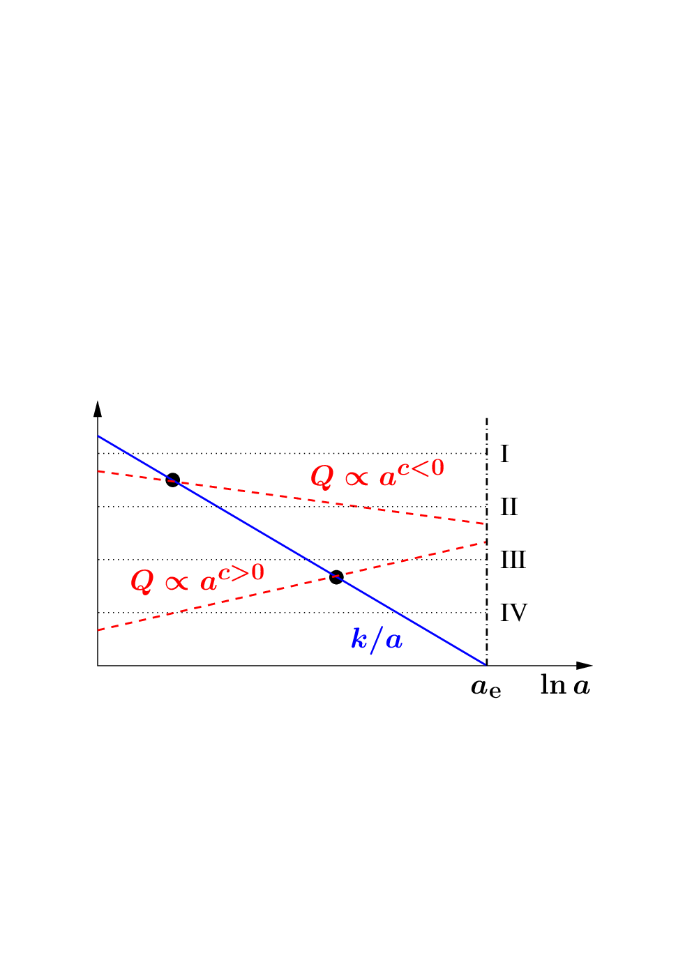
III.3.1 The Case I

This corresponds to the case when the inflationary Hubble parameter is represented by the uppermost dotted line in Fig. 1, i.e. $k/a_{\mathrm{x}}H\ll 1$ and $Q_{\mathrm{e}}/H\ll 1$ . In this regime the $Q$ term can be increasing as well as decreasing, i.e. $c>0$ or $c<0$ . We find the constants $C_{1}^{+}$ and $C_{2}^{+}$ by expanding Eqs. (39) and (40) for small values of $k/a_{\mathrm{x}}H$

	$\displaystyle C_{1}^{+}$	$\displaystyle=$	$\displaystyle-\frac{is_{c}}{3}\Gamma\left(\nu+1\right)\sqrt{\frac{k}{2a_{\mathrm{x}}H^{2}}}\left(\frac{k}{2\left\|c\right\|a_{\mathrm{x}}H}\right)^{-\nu}s_{1}^{+},$		(46)
	$\displaystyle C_{2}^{+}$	$\displaystyle=$	$\displaystyle-\frac{is_{c}}{3}\frac{\pi}{\Gamma\left(\nu\right)}\sqrt{\frac{k}{2a_{\mathrm{x}}H^{2}}}\left(\frac{k}{2\left\|c\right\|a_{\mathrm{x}}H}\right)^{\nu}s_{2}^{+},$		(47)

where

	$\displaystyle s_{1}^{+}$	$\displaystyle\equiv$	$\displaystyle 1-\left[3+\left\|c\right\|\left(s_{c}-1\right)\right]^{s_{c}}\left(\frac{k}{a_{\mathrm{x}}H}\right)^{-1-s_{c}},$		(48)
	$\displaystyle s_{2}^{+}$	$\displaystyle\equiv$	$\displaystyle 1-\left[3+\left\|c\right\|\left(s_{c}+1\right)\right]^{-s_{c}}\left(\frac{k}{a_{\mathrm{x}}H}\right)^{-1+s_{c}}.$		(49)

Note that, for an increasing $Q$ , $s_{1}^{+}\gg s_{2}^{+}$ , and for the decreasing one $s_{1}^{+}\ll s_{2}^{+}$ . In both cases, they are equal to

s_{1}^{+}\left(c>0\right)=s_{2}^{+}\left(c<0\right)\approx-3\left(\frac{k}{a_{\mathrm{x}}H}\right)^{-2}.

(50)

Expanding the Bessel function in Eq. (41) with $Q_{\mathrm{e}}/H\ll 1$ we find

w_{+}=a^{-3/2}\left[C_{1}^{+}\frac{1}{\Gamma\left(\nu+1\right)}\left(\frac{Q}{2\left|c\right|H}\right)^{\nu}-C_{2}^{+}\frac{\Gamma\left(\nu\right)}{\pi}\left(\frac{Q}{2\left|c\right|H}\right)^{-\nu}\right].

(51)

Inserting Eqs. (46), (47) and taking into account Eq. (50), we finally obtain

w_{+}=\frac{i}{\sqrt{2}}Hk^{-3/2}.

(52)

Using Eq. (45) we see that the spectrum of $w_{+}$ is flat

\mathcal{P}_{w_{+}}^{\left(\mathrm{I}\right)}=\left(\frac{H}{2\pi}\right)^{2}.

(53)

We apply the same method for calculating the power spectrum of the $w_{-}$ mode. In the limit of small $k/a_{\mathrm{x}}H$ constants $C_{1}^{-}$ and $C_{2}^{-}$ in Eqs. (43) and (44) become

	$\displaystyle C_{1}^{-}$	$\displaystyle=$	$\displaystyle-\frac{i}{3}\Gamma\left(\nu+1\right)\sqrt{\frac{k}{2a_{\mathrm{x}}H^{2}}}\left(\frac{k}{2\left\|c\right\|a_{\mathrm{x}}H}\right)^{-\nu}s_{1}^{-},$		(54)
	$\displaystyle C_{2}^{-}$	$\displaystyle=$	$\displaystyle\frac{i}{3}\frac{2}{\Gamma\left(\nu\right)}\sqrt{\frac{k}{2a_{\mathrm{x}}H^{2}}}\left(\frac{k}{2\left\|c\right\|a_{\mathrm{x}}H}\right)^{\nu}s_{2}^{-},$		(55)

where $s_{1}^{-}$ and $s_{2}^{-}$ are given by

	$\displaystyle s_{1}^{-}$	$\displaystyle\equiv$	$\displaystyle s_{c}-\left[3+\left\|c\right\|\left(s_{c}-1\right)\right]^{s_{c}}\left(\frac{k}{a_{\mathrm{x}}H}\right)^{-1-s_{c}},$		(56)
	$\displaystyle s_{2}^{-}$	$\displaystyle\equiv$	$\displaystyle s_{c}+\left[3+\left\|c\right\|\left(s_{c}+1\right)\right]^{-s_{c}}\left(\frac{k}{a_{\mathrm{x}}H}\right)^{-1+s_{c}}.$		(57)

One can see again that for $c>0$ , $s_{1}^{-}\gg s_{2}^{-}$ and vice versa. Also for each of these cases

s_{1}^{-}\left(c>0\right)=s_{2}^{-}\left(c<0\right)\approx-s_{c}3\left(\frac{k}{a_{\mathrm{x}}H}\right)^{-2}.

(58)

Next, expanding Eq. (41) for small $Q_{\mathrm{e}}/\left|c\right|H$ we find

w_{-}=a^{-3/2}\left[\frac{C_{1}^{-}}{\Gamma\left(\nu+1\right)}\left(\frac{Q_{\mathrm{e}}}{2\left|c\right|H}\right)^{\nu}+C_{2}^{-}\frac{\Gamma\left(\nu\right)}{2}\left(\frac{Q_{\mathrm{e}}}{2\left|c\right|H}\right)^{-\nu}\right].

(59)

It is easy to find that, using Eq. (58) and expressions for $C_{1}^{-}$ and $C_{2}^{-}$ in Eqs. (54) and (55), the mode function $w_{-}$ becomes

w_{-}=\frac{is_{c}}{\sqrt{2}}Hk^{-3/2}.

(60)

Thus the power spectrum is also flat and equal to

\mathcal{P}_{w_{-}}^{\left(\mathrm{I}\right)}=\left(\frac{H}{2\pi}\right)^{2}.

(61)

As we can see from Eqs. (53) and (61), the power spectra for both transverse modes are identical at first order in $Q_{\mathrm{e}}/H$ and are equal to the one of the light scalar field. This is not surprising as the equations of motion for $w_{+}$ and $w_{-}$ in Eq. (33) reduces to the one of the light scalar field. The spectral tilt of $\mathcal{P}_{w_{\pm}}$ , however, will differ from the scalar field case as the $Q\left(t,k\right)$ is a function of time and momentum.

To find the spectral tilt of $\mathcal{P}_{w_{\pm}}$ we expand the Bessel functions to the second order in $Q_{\mathrm{e}}/H$ . Let us consider $\mathcal{P}_{w_{+}}$ first. Then

	$\displaystyle J_{\nu}\left(\frac{Q}{\left\|c\right\|H}\right)$	$\displaystyle=$	$\displaystyle\frac{1}{\Gamma\left(1+\nu\right)}\left(\frac{Q}{2\left\|c\right\|H}\right)^{\nu}\left[1-\frac{1}{1+\nu}\left(\frac{Q}{2\left\|c\right\|H}\right)^{2}\right]+\mathcal{O}\left[\left(\frac{Q}{H}\right)^{\nu+4}\right],$		(62)
	$\displaystyle Y_{\nu}\left(\frac{Q}{\left\|c\right\|H}\right)$	$\displaystyle=$	$\displaystyle-\frac{\Gamma\left(\nu\right)}{\pi}\left(\frac{Q}{2\left\|c\right\|H}\right)^{-\nu}\left[1-\frac{1}{1-\nu}\left(\frac{Q}{2\left\|c\right\|H}\right)^{2}\right]+\mathcal{O}\left[\left(\frac{Q}{H}\right)^{\nu+4}\right].$		(63)

The above expression for $Y_{\nu}$ is valid only for $\nu>1$ . However, the $Y_{\nu}$ term in Eq. (36) is dominant only when this condition is satisfied. From the above, it is easy to infer that, to second order in $Q_{\mathrm{e}}/H$ , the power spectrum of $w_{+}$ is

\mathcal{P}_{w_{+}}=\left(\frac{H}{2\pi}\right)^{2}\left[1-\frac{4c}{3+2c}\left(\frac{Q_{\mathrm{e}}}{2\left|c\right|H}\right)^{2}\right].

(64)

Performing the same expansion for the hyperbolic Bessel functions we find

	$\displaystyle\mathcal{I}_{\nu}\left(\frac{Q}{\left\|c\right\|H}\right)$	$\displaystyle=$	$\displaystyle\frac{1}{\Gamma\left(1+\nu\right)}\left(\frac{Q}{2\left\|c\right\|H}\right)^{\nu}\left[1+\frac{1}{1+\nu}\left(\frac{Q}{2\left\|c\right\|H}\right)^{2}\right]+\mathcal{O}\left[\left(\frac{Q}{H}\right)^{\nu+4}\right],$		(65)
	$\displaystyle\mathcal{K}_{\nu}\left(\frac{Q}{\left\|c\right\|H}\right)$	$\displaystyle=$	$\displaystyle\frac{\Gamma\left(\nu\right)}{2}\left(\frac{Q}{2\left\|c\right\|H}\right)^{-\nu}\left[1+\frac{1}{1-\nu}\left(\frac{Q}{2\left\|c\right\|H}\right)^{2}\right]+\mathcal{O}\left[\left(\frac{Q}{H}\right)^{\nu+4}\right].$		(66)

With this result, the power spectrum of $w_{-}$ becomes

\mathcal{P}_{w_{-}}=\left(\frac{H}{2\pi}\right)^{2}\left[1+\frac{4c}{3+2c}\left(\frac{Q_{\mathrm{e}}}{2\left|c\right|H}\right)^{2}\right].

(67)

The two expressions for $\mathcal{P}_{w_{\pm}}$ above can be combined into one result

\mathcal{P}_{w_{\pm}}=\left(\frac{H}{2\pi}\right)^{2}\left[1\mp\varepsilon\frac{k}{H}\right],

(68)

where

\varepsilon\equiv\frac{a_{\mathrm{e}}^{2c}}{c\left(3+2c\right)}\,\frac{\dot{h}_{0}}{Hf_{0}}.

(69)

As it is clear from the above, the spectral dependence of the power spectra of $w_{+}$ and $w_{-}$ are the same but with opposite signs. The power spectrum of $\zeta$ in Eq. (5), on the other hand, is proportional only to the arithmetic average of $\mathcal{P}_{w_{+}}$ and $\mathcal{P}_{w_{-}}$ in which momentum dependence cancels out. Thus the vector field in this case may influence the spectral tilt of $\mathcal{P}_{\zeta}$ only at even higher order in $Q_{\mathrm{e}}/H\ll 1$ , which probably makes it undetectably small.

Spectral tilts of $\mathcal{P}_{w_{\pm}}$ do not modify $f_{\mathrm{NL}}$ significantly too. As can be seen from the definitions of the parameters $p$ and $q$ in Eq. (3) and the expressions for $f_{\mathrm{NL}}$ in Eqs. (12) - (14), the above spectral dependence influences $f_{\mathrm{NL}}$ only through the parameter $q$ . In this case, however, $q\left(k\right)\ll 1$ .

III.3.2 The Case II

Case II corresponds to when the $Q$ term dominates the $k/a$ one in Eq. (29) before horizon exit, but at the end of inflation $Q_{\mathrm{e}}\ll H$ . This is possible only if $Q$ is a decreasing function of time, that is $c<0$ . As discussed in subsection III.2, however, to set initial Bunch-Davies conditions the $k/a$ term in Eq. (29) must dominate initially. Therefore the $Q$ term must decrease slower than $k/a$ , putting the lower bound on $c>-1$ .

In the limit $k/a_{\mathrm{x}}H\gg 1$ , the constants $C_{1}^{+}$ and $C_{2}^{+}$ in Eqs. (39) and (40) become

C_{2}^{+}=-is_{c}C_{1}^{+}=-\frac{is_{c}}{2}\sqrt{\frac{\pi}{\left|c\right|H}}\mathrm{e}^{i\psi},

(70)

where

\psi\equiv\frac{k}{a_{\mathrm{x}}H}\left(1+\frac{1}{c}\right)-s_{c}\frac{2\nu+1}{4}\pi.

(71)

The equation for $w_{+}$ in the limit $Q_{\mathrm{e}}/H\ll 1$ is given in Eq. (51), with the constants $C_{1}^{+}$ and $C_{2}^{+}$ determined by Eq. (70). As $\nu$ is positive by definition, the second term on the RHS of Eq. (51) dominates. Inserting it into Eq. (45), we find

\mathcal{P}_{w_{+}}^{\left(\mathrm{II}\right)}=\left(2\left|c\right|\right)^{2\nu-1}\frac{\Gamma^{2}\left(\nu\right)}{\pi}\left(\frac{\dot{h}}{Hf}\right)^{-\nu}\left(\frac{k}{aH}\right)^{3-\nu}\left(\frac{H}{2\pi}\right)^{2}.

(72)

One notices that with $c=-1/2$ , $\nu=3$ and the power spectrum of $w_{+}$ is flat

\mathcal{P}_{w_{+}}^{\left(\mathrm{II}\right)}=\frac{4}{\pi}\left(\frac{\dot{h}}{Hf}\right)^{-3}\left(\frac{H}{2\pi}\right)^{2}.

(73)

Let’s consider the $w_{-}$ mode next. In the limit $k/a_{\mathrm{x}}H\gg 1$ the constants $C_{1}^{-}$ and $C_{2}^{-}$ become

	$\displaystyle\left\|C_{1}^{-}\right\|$	$\displaystyle=$	$\displaystyle\sqrt{\frac{\pi}{2\left\|c\right\|H}}\mathrm{e}^{-k/a_{\mathrm{x}}\left\|c\right\|H},$		(74)
	$\displaystyle\left\|C_{2}^{-}\right\|$	$\displaystyle=$	$\displaystyle\frac{1}{\sqrt{2\pi\left\|c\right\|H}}\mathrm{e}^{k/a_{\mathrm{x}}\left\|c\right\|H},$		(75)

and in the limit $Q_{\mathrm{e}}/H\ll 1$ the mode function $w_{-}$ is given in Eq. (59). Because $Q_{\mathrm{e}}/H\ll 1$ and $\left|C_{2}^{-}\right|\gg\left|C_{1}^{-}\right|$ the second term dominates and its contribution to the power spectrum is

\mathcal{P}_{w_{-}}^{\left(\mathrm{II}\right)}=\mathcal{P}_{w_{+}}^{\left(\mathrm{II}\right)}\frac{1}{2}\mathrm{e}^{\Theta^{\left(\mathrm{II}\right)}},

(76)

where

\Theta^{\left(\mathrm{II}\right)}\equiv\frac{2}{\left|c\right|}\left(\frac{\dot{h}}{Hf}\right)^{\frac{1}{2\left(c+1\right)}}\left(\frac{k}{aH}\right)^{\frac{1+2c}{2\left(c+1\right)}}.

(77)

Here again one can easily notice that, with $c=-1/2$ , the exponential amplification of the power spectrum $\mathcal{P}_{w_{-}}^{\left(\mathrm{II}\right)}$ is scale independent

\Theta^{\left(\mathrm{II}\right)}=4\frac{\dot{h}}{Hf}.

(78)

III.3.3 The Case III

Case III in Figure 1 corresponds to the situation when the $Q$ term takes over the $k/a$ term in Eq. (29) after horizon exit, but $Q$ is a growing function of time and becomes larger than $H$ at the end of inflation. We find the power spectra of $w_{+}$ and $w_{-}$ by the same method as in the previous two subsections.

Since Case III corresponds to $k/a_{\mathrm{x}}H\ll 1$ , constants $C_{1}^{+}$ and $C_{2}^{+}$ in this limit are given in Eqs. (46) and (47). While in the limit $Q_{\mathrm{e}}/H\gg 1$ , Eq. (36) for $w_{+}$ becomes

w_{+}=a^{-3/2}\sqrt{\frac{2\left|c\right|H}{\pi Q_{\mathrm{e}}}}\left[C_{1}^{+}\cos\left(\frac{Q_{\mathrm{e}}}{\left|c\right|H}-\frac{2\nu+1}{4}\pi\right)+C_{2}^{+}\sin\left(\frac{Q_{\mathrm{e}}}{\left|c\right|H}-\frac{2\nu+1}{4}\pi\right)\right].

(79)

For an increasing $Q$ , i.e. $c>0$ , $\left|C_{1}^{+}\right|\gg\left|C_{2}^{+}\right|$ and the first term in the above equation dominates. Using this and Eqs. (46) we find

\mathcal{P}_{w_{+}}^{\left(\mathrm{III}\right)}=\left(2\left|c\right|\right)^{1+2\nu}\frac{\Gamma^{2}\left(\nu+1\right)}{\pi}\left(\frac{k}{aH}\frac{\dot{h}_{\mathrm{e}}}{Hf_{\mathrm{e}}}\right)^{-\frac{c+3}{c}}\left(\frac{H}{2\pi}\right)^{2}\cos^{2}\Theta^{\left(\mathrm{III}\right)},

(80)

where

\Theta^{\left(\mathrm{III}\right)}\equiv\frac{Q_{\mathrm{e}}}{\left|c\right|H}-\frac{2\nu+1}{4}\pi.

(81)

As $c>0$ the power spectrum $\mathcal{P}_{w_{+}}$ in this case cannot be scale invariant.

The integration constants of the $w_{-}$ mode for $k/a_{\mathrm{x}}H\ll 1$ are given in Eqs. (54) and (55). Expanding Eq. (41) in the limit $Q_{\mathrm{e}}/H\gg 1$ we find

w_{-}=a^{-3/2}\sqrt{\frac{\left|c\right|H}{2\pi Q_{\mathrm{e}}}}\left(C_{1}^{-}\mathrm{e}^{Q_{\mathrm{e}}/\left|c\right|H}+\pi C_{2}^{-}\mathrm{e}^{-Q_{\mathrm{e}}/\left|c\right|H}\right).

(82)

For increasing $Q$ , the constants are $\left|C_{1}^{-}\right|\gg\left|C_{2}^{-}\right|$ and the first term dominates. Using this we find

\mathcal{P}_{w_{-}}^{\left(\mathrm{III}\right)}=\mathcal{P}_{w_{+}}^{\left(\mathrm{III}\right)}\frac{1}{4}\mathrm{e}^{2Q_{\mathrm{e}}/\left|c\right|H}.

(83)

Because $Q_{\mathrm{e}}/H\gg 1$ is a function of a wave-number $k$ , we see that the power spectrum of $w_{-}$ features an exponential, scale dependent amplification factor.

III.3.4 The Case IV

In the Case IV, $Q$ is always larger than the Hubble parameter during inflation. Such scenario corresponds to $k/a_{\mathrm{x}}\gg H$ and $Q_{\mathrm{e}}\gg H$ . We have already calculated the integration constants and the equations for the mode functions in the previous subsections. The expression for $w_{+}$ mode in the large $Q_{\mathrm{e}}$ limit is given in Eq. (79). While the constants $C_{1}^{+}$ and $C_{2}^{+}$ in the large $k/Ha_{\mathrm{x}}$ limit can be found in Eq. (70). With these equations it is easy to find the following solution for $w_{+}$

w_{+}=a^{-3/2}C_{1}^{+}\sqrt{\frac{2\left|c\right|H}{\pi Q_{\mathrm{e}}}}\mathrm{e}^{is_{c}\Theta^{\left(\mathrm{III}\right)}},

(84)

where the phase factor $\Theta^{\left(\mathrm{III}\right)}$ is defined in Eq. (81). Substituting this into Eq. (45), we find

\mathcal{P}_{w_{+}}^{\left(\mathrm{IV}\right)}=\left(\frac{\dot{h}}{Hf}\right)^{-1/2}\left(\frac{k}{aH}\right)^{5/2}\left(\frac{H}{2\pi}\right)^{2}.

(85)

As one can see this spectrum is very blue.

In an analogous way, we can compute the power spectrum of the $w_{-}$ mode, which in the large $Q_{\mathrm{e}}$ limit is given in Eq. (82). The integration constants $C_{1}^{-}$ and $C_{2}^{-}$ were calculated in Eqs. (74) and (75). Putting these expressions together we find

w_{-}=\frac{a^{-3/2}}{2\sqrt{Q_{\mathrm{e}}}}\left[\mathrm{e}^{\left(Q_{\mathrm{e}}-k/a_{\mathrm{x}}\right)/\left|c\right|H}+\mathrm{e}^{-\left(Q_{\mathrm{e}}-k/a_{\mathrm{x}}\right)/\left|c\right|H}\right].

(86)

When $Q$ is an increasing function of time, i.e. $c>0$ , then $Q_{\mathrm{e}}\gg k/a_{\mathrm{x}}$ and the first term in the above expression dominates. While, for $c<0$ , the second term dominates. With this solution, the spectrum of $w_{-}$ becomes

\mathcal{P}_{w_{-}}^{\left(\mathrm{IV}\right)}=\mathcal{P}_{w_{+}}^{\left(\mathrm{IV}\right)}\frac{1}{2}\mathrm{e}^{2\left(Q_{\mathrm{e}}-k/a_{\mathrm{x}}\right)/cH}.

(87)

Thus, again in this case we find that the power spectrum of $w_{-}$ has an exponential $k$ -dependent amplification.

III.3.5 Logarithmic $h$

The last two cases - logarithmic $h$ and constant $Q$ - are not shown in Figure 1. In the first, logarithmic $h$ case the time derivative of $h$ is constant during (quasi) de Sitter inflation:

\dot{h}=Hh_{0}\approx\mathrm{constant},

(88)

where $h_{0}$ is the initial value of $h$ . From the definition of the function $Q$ in Eq. (28) we notice that

Q\propto a^{-\left(1+\alpha\right)/2},

(89)

where $\alpha\equiv-1\pm 3$ is the scaling of the kinetic function $f\propto a^{\alpha}$ . While from the definition of $c$ in Eq. (34) we can see that the logarithmic scaling of $h$ corresponds to

c=\pm 3/2,

(90)

where $c=-3/2$ is for $\alpha=2$ . With negative $c$ the function $Q$ is decreasing. But in order to be able to impose the Bunch-Davies initial conditions $Q$ has to be decreasing slower than $k/a$ . Thus $c=-3/2$ is unviable. However, for $\alpha=-4$ , $c=3/2$ and we can use the results of subsections III.3.1, III.3.3 and III.3.4 to deduce the power spectrum.

III.3.6 Constant $Q$

For the constant $Q$ case, the equations of motion of both modes $w_{+}$ and $w_{-}$ in Eq. (29) reduce to the familiar equation of a massive scalar field. The difference, however, is that the effective “mass” in this case is scale dependent, $Q\propto k^{1/2}$ and for the $w_{-}$ mode this “mass” is tachyonic. For $Q\ll H$ , the power spectrum is well known for this type of equation

\mathcal{P}_{w_{\pm}}^{\left(\mathrm{const}\right)}=\left(\frac{H}{2\pi}\right)^{2}\left(\frac{k}{2aH}\right)^{3-2\nu_{\pm}},

(91)

where

\nu_{\pm}\equiv\sqrt{\frac{9}{4}\mp\left(\frac{Q}{H}\right)^{2}}.

(92)

We see that in the limit $Q\ll H$ , the spectrum is almost flat. It is also clear that both modes will have the same spectral tilt, but of the opposite sign: the spectrum of $w_{+}$ is slightly blue-tilted and red-tilted for $w_{-}$ . However, as discussed in Subsection III.3.1 this does not affect the spectral tilt of $\mathcal{P}_{\zeta}$ and makes a negligible contribution to $f_{\mathrm{NL}}$ .

III.3.7 Summary of the Subsection

We summarize the results of subsection III.3 in Table 1. There are two parameter spaces for producing a flat perturbation spectrum for both of transverse modes. First, this can be realised for any value of $c$ if the $Q$ term in Eq. (29) dominates the $k/a$ term after modes exit the horizon and if $Q$ stays smaller than $H$ until the end of inflation⁵⁵ 5 We assumed here $M\ll Q$ .. Such a vector field can generate statistical anisotropy in the curvature perturbation $\zeta$ which is consistent with the observational bounds. This can be realized, for example, using the vector curvaton scenario [1]. In this case the results of the vector curvaton scenario discussed in Ref. [19] are directly applicable⁶⁶ 6 The only difference are the additional constraints $k/a_{\mathrm{x}}H\ll 1$ and $Q_{\mathrm{e}}/H\ll 1$ .. But as both transverse modes acquire the same perturbation amplitude, the axial term in the Lagrangian will not have a detectable signature in the curvature perturbation in this parameter space.

However, in this paper we are also interested in a possibility of producing $\zeta$ with parity violating statistics. As shown in Sec. III.3.2 this can be realized if the function $Q$ scales as $c=-1/2$ and if it dominates $k/a$ term in Eq. (29) before horizon exit. Note, however, that $Q\propto k^{1/2}$ . Therefore the above discussion is valid only for some limited range of $k$ values. Particularly, $\mathcal{P}_{w_{+}}=\mathcal{P}_{w_{-}}=\left(H/2\pi\right)^{2}$ if $k/a_{\mathrm{x}}H\ll 1$ and $Q_{\mathrm{e}}\left(k\right)/H\ll 1$ . And parity violating perturbations are realized if the former bound is reversed and $c=-1/2$ . We study the latter case in more detail in Sec. IV.

	$\mathcal{P}_{w_{+}}$	$\mathcal{P}_{w_{-}}$
Case I	$\left(\frac{H}{2\pi}\right)^{2}$	$\mathcal{P}_{w_{+}}$
Case II	$\left(2\left\|c\right\|\right)^{2\nu-1}\frac{\Gamma^{2}\left(\nu\right)}{\pi}\left(\frac{\dot{h}_{\mathrm{e}}}{Hf_{\mathrm{e}}}\right)^{-\nu}\left(\frac{k}{a_{\mathrm{e}}H}\right)^{3-\nu}\left(\frac{H}{2\pi}\right)^{2}$	$\mathcal{P}_{w_{+}}\frac{1}{2}\mathrm{e}^{\Theta^{\left(\mathrm{II}\right)}}$
Case III	$\left(2\left\|c\right\|\right)^{1+2\nu}\frac{\Gamma^{2}\left(\nu+1\right)}{\pi}\left(\frac{k}{a_{\mathrm{e}}H}\frac{\dot{h}_{\mathrm{e}}}{Hf_{\mathrm{e}}}\right)^{-\frac{c+3}{c}}\left(\frac{H}{2\pi}\right)^{2}\cos^{2}\Theta^{\left(\mathrm{III}\right)}$	$\mathcal{P}_{w_{+}}\frac{1}{4}\mathrm{e}^{2Q_{\mathrm{e}}/\left\|c\right\|H}$
Case IV	$\left(\frac{\dot{h}_{\mathrm{e}}}{Hf_{\mathrm{e}}}\right)^{-1/2}\left(\frac{k}{a_{\mathrm{e}}H}\right)^{5/2}\left(\frac{H}{2\pi}\right)^{2}$	$\mathcal{P}_{w_{+}}\frac{1}{2}\mathrm{e}^{2\left(Q_{\mathrm{e}}-k/a_{\mathrm{x}}\right)/cH}$
$h\propto\ln a$	The same as cases I, III and IV with $c=3/2$
$Q=\mathrm{constant}$	$\mathcal{P}_{w_{\pm}}=\frac{4}{\pi}\Gamma^{2}\left(\nu_{\pm}\right)\left(\frac{H}{2\pi}\right)^{2}\left(\frac{k}{2a_{\mathrm{e}}H}\right)^{3-2\nu_{\pm}}$

Table 1: Summary of subsection III.3. In this table

\Theta^{\left(\mathrm{II}\right)}

is defined in Eq. (77),

\Theta^{\left(\mathrm{III}\right)}

is defined Eq. (81) and

\nu_{\pm}

in Eq. (92).

IV Statistically Anisotropic, Parity Violating Curvature Perturbation

IV.1 The Spectrum

In Subsection III.3.1 we found that the vector field acquires a scale invariant perturbation spectrum if the $Q$ term in Eq. (29) dominates the momentum term $k/a$ after the mode $k$ exits the horizon and $Q_{\mathrm{e}}\ll H$ at the end of inflation. In this case both modes, $w_{+}$ and $w_{-}$ , acquire perturbation spectrum equal to $\left(H/2\pi\right)^{2}$ . While in such a set-up the scale invariant curvature perturbation can also be generated, it does not give any signature of parity violation.

A more interesting case is studied in Subsection III.3.2. In this case, we find that the perturbation spectrum of the vector field is also scale invariant if the $Q$ term dominates the momentum one in Eq. (29) before the mode exits the horizon and if $Q$ is decaying during inflation as $Q\propto a^{-1/2}$ with $Q_{\mathrm{e}}\ll H$ at the end of inflation. From the definition of $Q$ in Eq. (28) we see that this scaling of $Q$ corresponds to

\frac{\dot{h}}{f}=\mathrm{constant}.

(93)

With the power law evolution of $f\propto a^{\alpha}$ the above condition implies that $h$ also evolves according to the same power law $h\propto a^{\alpha}$ ⁷⁷ 7 Remember that we assume (quasi) de Sitter inflation, i.e. $H\approx\mathrm{constant}$ ., where $\alpha=-1\pm 3$ . In view of this, we can rewrite the Lagrangian in Eq. (15) as

\mathcal{L}=-\frac{1}{4}f\left(F_{\mu\nu}F^{\mu\nu}+\vartheta F_{\mu\nu}\tilde{F}^{\mu\nu}\right)+\frac{1}{2}m^{2}A_{\mu}A^{\mu},

(94)

where

\vartheta\equiv\frac{h}{f}=\mathrm{constant}.

(95)

Then a vector field with the Lagrangian in Eq. (94) will acquire a flat perturbation spectrum if the $Q^{2}=\left|\alpha\vartheta\right|Hk/a$ term dominates the $\left(k/a\right)^{2}$ term in Eq. (29) before the mode exits the horizon. In the case when $Q\propto a^{-1/2}$ this happens at a scale factor $a_{\mathrm{x}}$ given by⁸⁸ 8 The moment $k/a_{\mathrm{x}}$ is represented by black dots in Figure 1.

\frac{k}{Ha_{\mathrm{x}}}=\frac{\dot{h}}{Hf}=\left|\alpha\vartheta\right|.

(96)

From this we see that the value of $k/a_{\mathrm{x}}$ does not depend neither on time nor on wave-number $k$ .

To calculate the perturbation spectrum of the vector field we used Bunch-Davies initial conditions in Subsection III.2. These initial conditions are valid in the limit where the curvature of space-time can be neglected and quantum fields are effectively described by the quantum theory of free fields. The first requirement is fulfilled for modes deep within the horizon, while the standard quantum field theory can be applied for modes which are not too close to the Planck scale, and the mode can be considered to be of an effectively free field if the $k/a$ term in Eq. (29) dominates. Using Eq. (96) we find that these requirements constrain the value of $\vartheta$ as

1\ll\left|\alpha\vartheta\right|\ll\frac{m_{\mathrm{Pl}}}{H}.

(97)

Because the parameter $\alpha$ is of order one, we see that the scale invariant vector field perturbation spectrum is achieved if the parity violating constant $\vartheta$ is much larger than unity. Then the spectra of modes $w_{-}$ and $w_{+}$ from Eqs. (73) and (76) can be written as

	$\displaystyle\mathcal{P}_{w_{+}}$	$\displaystyle=$	$\displaystyle\frac{4}{\pi}\left\|\alpha\vartheta\right\|^{-3}\left(\frac{H}{2\pi}\right)^{2};$		(98)
	$\displaystyle\mathcal{P}_{w_{-}}$	$\displaystyle=$	$\displaystyle\frac{4}{\pi}\left\|\alpha\vartheta\right\|^{-3}\left(\frac{H}{2\pi}\right)^{2}\frac{\mathrm{e}^{4\left\|\alpha\vartheta\right\|}}{2}.$		(99)

Note, that due to Eq. (97) the spectrum of $w_{+}$ is suppressed with respect to the standard light scalar field result.

For the expressions in Eqs. (98) and (99) to be valid, the $Q$ term must also be much smaller than $H$ by the end of inflation, $Q_{\mathrm{e}}\ll H$ . It follows from Eq. (96) that this implies

\left|\alpha\vartheta\right|\ll\frac{a_{\mathrm{e}}H}{k},

(100)

which must hold at least for cosmological scales. Assuming the observable inflation to last at least 50 e-folds, this bound is much weaker than the one in Eq. (97) for any realistic model of inflation.

If for the largest $k$ modes this bound is violated, we are back to the Case IV in Figure 1, which was discussed in Subsection III.3.4. As one can see in Eqs. (85) and (87), the spectra of both modes are very blue $\mathcal{P}_{w_{\pm}}\propto k^{5/2}$ . As the $\mathcal{P}_{w_{-}}$ is also exponentially enhanced by $\exp\left(4\left|\alpha\vartheta\right|\right)$ one may worry about the overproduction of the primordial black holes in such a scenario. The summary of various cosmological constraints on the abundance of the primordial black holes can be found in Ref. [38]. On practically all scales the bound correspond to $\mathcal{P}_{\zeta}\lesssim 10^{-2}$ for the Gaussian perturbation. If the perturbation is non-Gaussian then the bound becomes

\mathcal{P}_{\zeta}\left(k_{\mathrm{peak}}\right)\lesssim 10^{-3}\;\mathrm{or}\;1,

(101)

where the lower bound is for the positive non-Gaussianity and the upper bound is for the negative non-Gaussianity [39]. The contribution of the vector field to the spectrum of $\zeta$ is $N_{W}^{2}\mathcal{P}_{w_{-}}$ , where $N_{W}$ is defined in Eq. (4). From COBE normalization this contribution has to be $\lesssim 10^{-9}$ for cosmological scales. From Eqs. (98) and (99) $\mathcal{P}_{w_{-}}\gg\mathcal{P}_{w_{+}}$ and thus the spectrum of $\zeta$ is

N_{W}^{2}\frac{2}{\pi}\left|\alpha\vartheta\right|^{-3}\left(\frac{H}{2\pi}\right)^{2}\mathrm{e}^{4\left|\alpha\vartheta\right|}\lesssim 10^{-9},

(102)

for cosmological scales.

The spectrum of modes which violate the bound in Eq. (100) is given in Eq. (87). The blue spectrum peaks at the largest $k$ value, which corresponds to the horizon size at the end of inflation. Thus setting $k_{\mathrm{peak}}/a_{\mathrm{e}}H\approx 1$ and using Eq. (87) we can write the bound in Eq. (101) as

\frac{1}{2}N_{W}^{2}\left|\alpha\vartheta\right|^{-1/2}\left(\frac{H}{2\pi}\right)^{2}\mathrm{e}^{4\left|\alpha\vartheta\right|}\lesssim 10^{-3}\;\mathrm{or}\;1,

(103)

where we also used the fact that $k/a_{\mathrm{x}}\gg Q_{\mathrm{e}}$ for $c<0$ . Using Eq. (102) this becomes

\left|\alpha\vartheta\right|<10^{2}\;\mathrm{or}\;10^{4}.

(104)

As shown in Subsection (III.1), the equation of motion for the longitudinal mode of the vector field perturbation is not affected by the axial term. Thus the results of Ref. [19] for this mode can also be used directly in our case. It was found that the spectrum of the longitudinal mode is

\mathcal{P}_{\|}=\left(\frac{3H}{M_{\mathrm{e}}}\right)^{2}\left(\frac{H}{2\pi}\right)^{2},

(105)

where $M$ is an effective mass of the vector field defined in Eq. (26) and the index ‘ $\mathrm{e}$ ’ indicates that it is evaluated at the end of inflation. In these works it was also found that the spectrum of transverse modes are unaffected by the mass term if the field is light.

The predominantly parity violating perturbation will be generated if $\mathcal{P}_{w_{-}}>\mathcal{P}_{\|}$ . Comparing Eqs. (99) and (105) we find the condition for this to be

\left|\alpha\vartheta\right|^{-3}\mathrm{e}^{4\left|\alpha\vartheta\right|}>\left(\frac{3H}{M_{\mathrm{e}}}\right)^{2}.

(106)

Taking into account the bound in Eq. (104) one sees that the above condition can be easily satisfied even for extremely small values of $M_{\mathrm{e}}$ .

Results for the power spectrum given in Eqs. (98) and (99) are valid if the vector field is light during inflation. If this is not the case, and the field becomes heavy before the end of inflation, it starts oscillating and the amplitude of the spectrum decreases by $\frac{1}{2}\left(3H/M\right)^{2}$ [19]. As can be seen from the definition of the effective mass $M$ in Eq. (26) it can grow only if $\alpha=-4$ . In view of this we can rewrite Eqs. (98) and (99) as

	$\displaystyle\mathcal{P}_{w_{+}}$	$\displaystyle=$	$\displaystyle\frac{1}{16\pi}\left\|\vartheta\right\|^{-3}\left(\frac{H}{2\pi}\right)^{2}\frac{1}{2}\mathrm{min}\left\{1,\frac{3H}{M_{\mathrm{e}}}\right\}^{2};$		(107)
	$\displaystyle\mathcal{P}_{w_{-}}$	$\displaystyle=$	$\displaystyle\frac{1}{16\pi}\left\|\vartheta\right\|^{-3}\left(\frac{H}{2\pi}\right)^{2}\frac{\mathrm{e}^{16\left\|\vartheta\right\|}}{4}\mathrm{min}\left\{1,\frac{3H}{M_{\mathrm{e}}}\right\}^{2}.$		(108)

IV.2 The Vector Curvaton

So far we have discussed the perturbation of the vector field. One way a vector field can generate or contribute to the primordial curvature perturbation $\zeta$ is via the vector curvaton scenario [1]. In this scenario it is assumed that the vector field is light during inflation, at least while the cosmological scales exit the horizon. To avoid excessive anisotropic expansion of the Universe, the energy density of the light vector field has to be subdominant. After inflation, when the vector field becomes heavy, it oscillates with a very high frequency and behaves as preasureless, isotropic matter. The energy density of such matter decays slower than the radiation, and thus the vector field can dominate and generate the total of $\zeta$ or nearly dominate and generate a contribution to $\zeta$

\zeta=\left(1-\hat{\Omega}_{W}\right)\zeta_{\mathrm{rad}}+\hat{\Omega}_{W}\zeta_{W},

(109)

where $\hat{\Omega}_{W}$ is defined in Eq. (10) and $\zeta_{W}$ is the vector field contribution to the curvature perturbation $\zeta$ . If the vector field perturbation spectrum is statistically anisotropic, so is the spectrum of $\zeta$ [5, 6].

In Ref. [19] a vector curvaton scenario was studied with the Lagrangian in Eq. (94) and $\vartheta=0$ . Bounds derived in these references also apply to the current scenario as the axial term with $\vartheta\neq 0$ does not contribute to the homogeneous values of fields and, therefore, to the homogeneous value of the energy density. This is because for the homogenised vector field, $F_{ij}=0$ , where $i,j$ denote spatial components. The axial term is proportional to $\epsilon^{\mu\nu\rho\sigma}F_{\mu\nu}F_{\rho\sigma}$ . This means that, it cannot include any term featuring simultaneously two factors of the form $F_{0i}=-F_{i0}=\dot{A}$ , which is the only non-zero component of the field strength tensor. Thus to find the constraint on the energy scale of inflation we can use the expression for the Hubble parameter found in Ref. [19]

\frac{H}{m_{\mathrm{Pl}}}\sim\Omega_{\mathrm{W}}^{1/2}\zeta_{W}\mathrm{min}\left\{1;\frac{M_{\mathrm{e}}}{H_{*}}\right\}^{-1/3}\mathrm{min}\left\{1;\frac{\hat{m}}{\Gamma}\right\}^{1/12}\left(\frac{\mathrm{max}\left\{\Gamma_{W};H_{\mathrm{dom}}\right\}}{\Gamma}\right)^{1/4}.

(110)

In this equation $H$ is the inflationary Hubble parameter, $\Omega_{\mathrm{W}}$ is defined in Eq. (11), $\Gamma$ and $\Gamma_{W}$ are the inflaton and vector field decay rates and $H_{\mathrm{dom}}$ is the value of the Hubble parameter after inflation, when the oscillating curvaton dominates over the radiation bath, if it does not decay earlier.

With the axial term the dominant contribution to the vector field perturbation comes from the $w_{-}$ term, thus $\mathcal{P}_{w_{-}}\gg\mathcal{P}_{w_{+}},\;\mathcal{P}_{\|}$ and $\mathcal{P}_{+}\approx\frac{1}{2}\mathcal{P}_{w_{-}}$ . Using Eq. (8) we find

g_{\zeta}\simeq-\frac{1}{2}\frac{N_{W}^{2}\mathcal{P}_{w_{-}}}{\mathcal{P}_{\zeta}^{\mathrm{iso}}}.

(111)

Also, using the fact that the anisotropic contribution to the power spectrum of $\zeta$ must be subdominant [10] (cf. Eq. (1)), to the first order we can write

\frac{\zeta^{2}}{\delta W^{2}}\simeq\frac{\mathcal{P}_{\zeta}^{\mathrm{iso}}}{\mathcal{P}_{w_{-}}},

(112)

where we also used the fact that the dominant contribution to the vector field perturbation is from the $w_{-}$ mode. Combining the above two equations we find

N_{W}^{2}\delta W^{2}\simeq-2g_{\zeta}\zeta^{2}.

(113)

Comparing the $\delta N$ formula in Eq. (4) and the equation for $\zeta$ in the curvaton scenario in Eq. (109) we can also write

N_{W}\delta W=\hat{\Omega}_{W}\zeta_{W}.

(114)

Inserting this into Eq. (113) we get

\zeta\sim\frac{\Omega_{\mathrm{W}}\zeta_{W}}{\sqrt{-g_{\zeta}}},

(115)

which can be used in Eq. (110) to find the lower bound of the inflationary Hubble parameter. In Ref. [19] it was shown that the lowest decay rate of the vector field is through the gravitational decay, which gives $\mathrm{max}\left\{\Gamma_{W};H_{\mathrm{dom}}\right\}\geq M_{\mathrm{e}}^{3}/m_{\mathrm{Pl}}^{2}$ . Using this and Eq. (115) we find the bound on the inflationary Hubble parameter $H$

\frac{H}{m_{\mathrm{Pl}}}>\left(-\frac{g_{\zeta}\zeta^{2}}{\Omega_{W}}\right)^{1/2}\left(\frac{M_{\mathrm{e}}}{m_{\mathrm{Pl}}}\right)^{3/4}\left(\frac{\Gamma}{m_{\mathrm{Pl}}}\right)^{-1/4}\mathrm{min}\left\{1;\frac{M_{\mathrm{e}}}{H_{*}}\right\}^{-1/3}\mathrm{min}\left\{1;\frac{\hat{m}}{\Gamma}\right\}^{1/12}.

(116)

As we can see from this inequality the bound is maximised if the Universe undergoes prompt reheating, that is $\Gamma\rightarrow H_{*}$ . Also note, that the bound on $H_{*}$ is maximised for the smallest value of the effective mass of the vector field $M_{\mathrm{e}}$ . Requiring that the vector field decays before the Big Bang Nucleosynthesis (BBN) gives $M_{\mathrm{e}}\gtrsim 10^{4}\,\mathrm{GeV}$ [19]. Inserting these limits into (116) and using the fact that $\Omega_{W}<1$ , the bound on $H_{*}$ and inflationary energy scale $V_{*}^{1/4}$ becomes

H>\sqrt{-g_{\zeta}}\,10^{6}\,\mathrm{GeV}\quad\Leftrightarrow\quad V_{\mathrm{inf}}^{1/4}>\left(-g_{\zeta}\right)^{1/4}\,10^{12}\,\mathrm{GeV}.

(117)

Also from the results in Ref. [19] the constraint on the mass of the vector field is

10\,\mathrm{TeV}\lesssim M_{\mathrm{e}}\lesssim 10^{6}H,

(118)

where the bound in Eq. (117) is saturated with the lower bound in Eq. (118).

From the above two constraints it is clear that there is an ample parameter space for this scenario to be realised.

IV.3 The Parity Violating Non-Gaussianity

As we saw in Section II to calculate $f_{\mathrm{NL}}$ it is convenient to use parameters $p$ and $q$ defined in Eq. (3). Because $\mathcal{P}_{w_{-}}$ is exponentially larger than both $\mathcal{P}_{w_{+}}$ and $\mathcal{P}_{\|}$ , $p$ and $q$ are equal to

p\approx-1\;\mathrm{and}\;\left|q\right|\approx 1.

(119)

The sign of $q$ is determined by the sign of $\alpha\vartheta$ . Following the definitions of $w_{+}$ and $w_{-}$ after Eq. (29) we find that $q\approx-1$ if $\alpha\vartheta>0$ and $q\approx+1$ otherwise.

The value of $\left|p\right|\approx 1$ violates observational bounds on the anisotropy in the spectrum. Thus, as discussed in Section (II), the vector field contribution to $\zeta$ must be subdominant, i.e. $\xi<1$ , which gives

g_{\zeta}\approx-\xi\quad\mathrm{and}\quad\hat{\Omega}_{W}\approx\frac{3}{4}\Omega_{W}.

(120)

Putting the above values of $p$ , $q$ , $\xi$ and $\hat{\Omega}_{W}$ in Eqs. (12)-(14) we find

$\displaystyle\frac{6}{5}f_{\mathrm{NL}}^{\mathrm{eql}}$	$\displaystyle=$	$\displaystyle 3\frac{g_{\zeta}^{2}}{\Omega_{W}}\left(1-\frac{3}{4}W_{\perp}^{2}\right),$	(121)
$\displaystyle\frac{6}{5}f_{\mathrm{NL}}^{\mathrm{sqz}}$	$\displaystyle=$	$\displaystyle 2\frac{g_{\zeta}^{2}}{\Omega_{W}}\left(1-W_{\perp}^{2}-i\penalty\ \mathrm{sgn}(\alpha\vartheta)W_{\perp}\sqrt{1-W_{\perp}^{2}}\sin\omega\right),$	(122)
$\displaystyle\frac{6}{5}f_{\mathrm{NL}}^{\mathrm{flt}}$	$\displaystyle=$	$\displaystyle\frac{4}{5}\frac{g_{\zeta}^{2}}{\Omega_{W}}\left(1-\cos^{2}\varphi W_{\perp}^{2}\right),$	(123)

where $\mathrm{sgn}(\alpha\vartheta)$ is the sign of $\alpha\vartheta$ . As $\mathcal{P}_{w_{-}}\gg\mathcal{P}_{\|}$ , the above result is valid for both: the light vector field and the one which becomes heavy at the end of inflation.

The shape of $f_{\mathrm{NL}}$ given in Eqs. (121)-(123) provides a smoking-gun signature for this model. It is easy to see that the maximum values of $f_{\mathrm{NL}}$ in different configurations are related as

\left.\frac{1}{3}f_{\mathrm{NL}}^{\mathrm{eql}}\right|_{\rm max}=\left.\mathrm{Re}\left[\frac{1}{2}f_{\mathrm{NL}}^{\mathrm{sqz}}\right]\right|_{\rm max}=\left.\frac{5}{4}f_{\mathrm{NL}}^{\mathrm{flt}}\right|_{\rm max},

(124)

while only $f_{\mathrm{NL}}^{\mathrm{eql}}$ has a non-vanishing minimum value of $3/4$ .

V Concrete examples

In this section we consider some specific models motivated by particle physics, which can provide a flat vector field perturbation spectrum with the use of the axial term $\propto F\tilde{F}$ . But before going into the models it is important to point out again that the axial term does not affect the dynamics of the homogenised fields. Thus, we will ignore this term when discussing the dynamics of the homogenised scalar and vector fields.

V.1 String inspired model

In string theory the gauge kinetic function and the coupling of the axial term are of the following form: $f={\rm Re}{\cal F}$ and $h={\rm Im}{\cal F}$ , where ${\cal F}$ is some complex holomorphic function of the moduli fields. Thus, the gauge field content of the model is

{\cal L}=-\frac{1}{4}({\rm Re}{\cal F})F_{\mu\nu}F^{\mu\nu}+\frac{1}{2}m^{2}A_{\mu}A^{\mu}+C\,({\rm Im}{\cal F})F_{\mu\nu}\tilde{F}^{\mu\nu}.

(125)

The simplest form for ${\cal F}$ is ${\cal F}\propto e^{-bT}$ , for large values of the modulus $T$ in Planck mass units ( $b=\,$ constant). Writing $T$ in terms of the real fields $\phi$ and $\sigma$ as $T=\phi+i\sigma$ and reinstating the Planck mass we find

\left.\begin{array}[]{l}f=e^{-b\phi/m_{\mathrm{Pl}}}\cos(b\sigma/m_{\mathrm{Pl}})\\ \\ h=Ce^{-b\phi/m_{\mathrm{Pl}}}\sin(b\sigma/m_{\mathrm{Pl}})\end{array}\right\}\Rightarrow\frac{h}{f}=\vartheta=C\tan(b\sigma/m_{\mathrm{Pl}}),

(126)

where $\vartheta$ was defined in Eq. (95). If the axion $\sigma$ remains frozen during inflation with $\sigma\simeq\mathrm{constant}$ then we have $\vartheta=\mathrm{constant}$ , i.e. $f\propto h\propto a^{\alpha}$ and $c=-\frac{1}{2}$ . This is a very realistic possibility because the axion mass is protected by the approximate U(1) symmetry and can be very small, much smaller than $H$ during inflation. Note that we have not clarified whether $\phi$ and $\sigma$ are canonically normalised fields. Indeed, if the Kähler potential has a non-trivial dependence on these fields they will not be canonically normalised. However, this does not change the result above, that is $c=-\frac{1}{2}$ .

In the opposite limit of small $T$ the dependence of ${\cal F}$ on the modulus is logarithmic. For toroidal compactifications the Kähler potential is of the form $K=-3\ln(T+\bar{T})$ in Planck units, where $T$ is a complex structure modulus here. This means that $K=-3m_{\mathrm{Pl}}^{2}\ln(2\phi/m_{\mathrm{Pl}})$ . Hence, the kinetic term of the $\phi$ field is non-canonical and it reads

{\cal L}_{{\rm kin}}=K_{\phi\phi}\partial_{\mu}\phi\partial^{\mu}\phi=3g^{\mu\nu}\left(\frac{m_{\mathrm{Pl}}}{\phi}\right)^{2}\partial_{\mu}\phi\partial_{\nu}\phi\,.

In view of this we can define the canonically normalised scalar field $\Phi$ as $\ln(\phi/m_{\mathrm{Pl}})=\frac{1}{\sqrt{6}}\Phi/m_{\mathrm{Pl}}$ . Thus, if we ignore the axion, the gauge kinetic function is $f\propto{\rm Re}{\cal F}\propto(\ln\phi)^{n}\propto\Phi^{n}$ , i.e. it has a power-law dependence on the canonically normalised field $\Phi$ .

In summary, provided we ignore the axion (presumed frozen), string theory suggests that $h/f=\mathrm{constant}$ . The functional dependence of $f$ and $h$ on the varying modulus (which could be the inflaton) depends on the (unknown) compactification scheme but both exponential and power-law dependence is reasonable.

The condition $k/a_{\mathrm{x}}\gg H$ is ensured by the lower bound in Eq. (97), i.e. $\vartheta\gg 1/4$ with $\alpha=-4$ . From Eq. (126), assuming $C\sim 1$ , we see that this condition translates into the lower bound for $\sigma$

\frac{\sigma}{m_{\mathrm{Pl}}}\gg 10^{-1}/b\,.

(127)

Thus, assuming $b\sim 1$ , this condition is satisfied provided the value of the (frozen) axion is comparable to the Planck scale, but this can be relaxed if $C\gg 1$ (see for example Ref. [29]). The upper bound on $\vartheta$ , which limits the overproduction of primordial black holes and is given in Eq. (104), translates into

C\tan\left(\frac{b\sigma}{m_{\mathrm{Pl}}}\right)<10^{2}\>\mathrm{or}\>10^{4}.

(128)

As was mentioned before, this also ensures that $Q_{\mathrm{e}}\ll H$ for cosmological scales, as the latter is a weaker constraint. If the two bounds in Eqs. (127) and (128) are satisfied, it is possible in this set up to generate parity violating $\zeta$ with a flat power spectrum, as discussed in Section IV.

V.2 The orthogonal axion

This model is of the form

$\displaystyle{\cal L}$	$\displaystyle=$	$\displaystyle D_{\mu}\Phi(D^{\mu}\Phi)^{*}-V(\Phi)-\frac{1}{4}fF_{\mu\nu}F^{\mu\nu}+\hat{c}e^{2}\hat{\theta}F_{\mu\nu}\tilde{F}^{\mu\nu}$	(129)
	$\displaystyle=$	$\displaystyle\frac{1}{2}\partial_{\mu}\phi\partial^{\mu}\phi+\frac{1}{2}\partial_{\mu}\sigma\partial^{\mu}\sigma-V(\phi)-V(\sigma)-$
		$\displaystyle-\frac{1}{4}fF_{\mu\nu}F^{\mu\nu}+\frac{1}{2}e^{2}\phi^{2}A_{\mu}A^{\mu}+\hat{c}e^{2}\frac{\sigma}{\phi_{0}}F_{\mu\nu}\tilde{F}^{\mu\nu},$

where $D_{\mu}\equiv\partial_{\mu}+ieA_{\mu}$ and $f$ is modulated by some inflaton field but $\phi$ or $\sigma$ are not it. Comparing the above Lagrangian with Eq. (15) we see that

h=-4\hat{c}e^{2}\frac{\sigma}{\phi_{0}}

(130)

in this model. To have some time-dependence for the axion $\sigma\equiv\hat{\theta}\phi_{0}$ we need its mass to be comparable to the Hubble parameter. Thus, we consider modular inflation with $H\sim\,$ TeV and we assume that $\sigma$ is an axion field, orthogonal to the QCD axion in supersymmetric realisations of the Peccei-Quinn symmetry, which employ a non-renormalisable superpotential for the Peccei-Quinn fields [40, 41]. This construction also solves the $\mu$ -problem of supersymmetry.

The superpotential is of the form

W=\frac{\kappa}{n+3}\frac{\Phi^{n+3}}{m_{\mathrm{Pl}}^{n}}\,,

(131)

where $\Phi=(\phi/\sqrt{2})\exp(i\hat{\theta}/\sqrt{2})$ , with $\hat{\theta}\equiv\sigma/\phi_{0}$ with $\phi_{0}$ being the Peccei-Quinn breaking scale given by

\phi_{0}=2\left(\frac{m_{\mathrm{Pl}}^{n}m_{\phi}}{\sqrt{2}\kappa}\right)^{1/(n+1)},

(132)

where $m_{\phi}\sim\,$ TeV is the tachyonic soft mass of the radial field $\phi$ , which breaks the Peccei-Quinn symmetry. The above is obtained by minimising

V(\phi)=V_{0}-\frac{1}{2}m_{\phi}^{2}\phi^{2}+\frac{\kappa^{2}}{2^{n+2}}\frac{\phi^{2(n+2)}}{m_{\mathrm{Pl}}^{2n}}\,,

(133)

where $V_{0}$ is some density scale. The orthogonal axion potential is

V(\sigma)=(\phi m_{\sigma})^{2}[1-\cos(\sigma/\phi)]\,.

(134)

The above potential is due to the soft A-term in the scalar potential,⁹⁹ 9 $\delta V_{{\rm A-term}}={\cal A}(W+W^{*})$ for a monomial superpotential. which gives the following value for the mass of the orthogonal axion:

m_{\sigma}^{2}=\kappa{\cal A}\frac{(\phi/\sqrt{2})^{n+1}}{m_{\mathrm{Pl}}^{n}}\,,

(135)

with ${\cal A}\sim\,$ TeV being the coefficient of the A-term. If the radial field assumes its vacuum value $\phi=\phi_{0}$ (i.e. it is not rolling down the radial direction) then the axion mass becomes

m_{\sigma}^{2}=2^{(n-2)/2}{\cal A}m_{\phi}\;.

(136)

We assume that, during inflation, the axion is very close to the origin and rolls down near a local minimum approaching the origin. Then we can write

\frac{\partial V(\sigma)}{\partial\sigma}=m_{\sigma}^{2}\phi_{0}\sin(\sigma/\phi_{0})\simeq m_{\sigma}^{2}\sigma\,.

(137)

Using the above, the axion’s equation of motion is

\ddot{\sigma}+3H\dot{\sigma}+m_{\sigma}^{2}\sigma\simeq 0\,,

(138)

whose growing mode solution is

\sigma\propto\exp\left\{-\frac{3}{2}\left[1-\sqrt{1-\left(\frac{2}{3}\frac{m_{\sigma}}{H}\right)^{2}}\right]Ht\right\}\propto a^{-\frac{3}{2}\left[1-\sqrt{1-\left(\frac{2}{3}\frac{m_{\sigma}}{H}\right)^{2}}\right]}.

(139)

Thus, if we denote

h\propto a^{\gamma}

(140)

from Eq. (139) we find

\gamma=-\frac{3}{2}\left[1-\sqrt{1-\left(\frac{2}{3}\frac{m_{\sigma}}{H}\right)^{2}}\right]\;\Rightarrow\;c=\frac{3}{4}\left[1+\sqrt{1-\left(\frac{2}{3}\frac{m_{\sigma}}{H}\right)^{2}}\right]>0\,,

(141)

where we also considered Eqs. (28) and (34) which suggest $2c=\gamma+3$ . If $m_{\sigma}\ll H$ then $\gamma\approx\frac{1}{3}(\frac{m_{\sigma}}{H})^{2}\ll 1\Rightarrow c\simeq 3/2$ , i.e. $\sigma$ slow-rolls (and $h\propto\ln a$ ). In fact, $\sigma$ is practically frozen, in which case there is no parity violation. For this reason we do not consider that the radial field is still rolling with $\phi\ll\phi_{0}$ , neither do we assume that the tachyonic mass of the radial field is suppressed by some supergravity correction so that $(m_{\phi}^{2})_{{\rm eff}}=m_{\phi}^{2}-\tilde{c}H^{2}\ll m_{\phi}^{2}\sim 1\,$ TeV, as in Ref. [41]. Both these possibilities would result in $m_{\sigma}\ll H\sim 1\,$ TeV. Therefore, we should assume that the Peccei-Quinn symmetry is fully broken with $\phi=\phi_{0}$ and $m_{\phi}\sim 1\,$ TeV, such that $m_{\sigma}\sim\sqrt{{\cal A}m_{\phi}}\sim H\sim 1\,$ TeV, according to Eq. (136).

The above imply that the mass of the physical vector field is

M\equiv\frac{m_{A}}{\sqrt{f}}=\frac{e\phi_{0}}{\sqrt{f}}\propto a^{2}.

(142)

Thus, the longitudinal component of the vector field exists and, if it undergoes particle production, it will not obtain a scale-invariant spectrum. We need to check whether the longitudinal component spoils the model.

From Eqs. (132) and (142) we find

\frac{M}{H}\sim e\left(\frac{m_{\mathrm{Pl}}}{m_{3/2}}\right)^{n/(n+1)}e^{-2N}\sim e\times 10^{15n/(n+1)}e^{-2N},

(143)

where $m_{3/2}\sim 1\,$ TeV stands for the weak scale (gravitino mass¹⁰¹⁰ 10 for gravity mediated supersymmetry breaking.) and we considered that, at the end of inflation, $f\rightarrow 1$ . Firstly, we need to verify that the field is light when the cosmological scales exit the horizon. The vector field becomes heavy (and begins oscillating) when $M\sim H$ . The earliest time for this to happen can be found by taking $e=1$ and $n\rightarrow\infty$ in the above. We obtain $N_{{\rm osc}}^{{\rm max}}\simeq\frac{15}{2}\ln 10\simeq 17$ , which corresponds to much later times than the exit of the cosmological scales.¹¹¹¹ 11 $N_{*}\simeq 50$ for prompt reheating with $V_{{\rm\textrm{inf}}}^{1/4}\sim\sqrt{m_{\mathrm{Pl}}m_{3/2}}$ .

Secondly, we need to ascertain that the vector field, after it begins oscillating, survives until the end of inflation at least, so that it can have some hope to affect the curvature perturbation in the Universe. The decay rate of the vector field is $\Gamma_{W}=\frac{e^{2}}{8\pi}M\propto a^{2}$ . Requiring that $\Gamma_{W}\mbox{\raisebox{-3.87495pt}{\penalty\ $\stackrel{{\scriptstyle\mbox{$<$}}}{{\sim}}$\penalty\ }}H$ at the end of inflation produces the constraint

e\mbox{\raisebox{-3.87495pt}{\penalty\ $\stackrel{{\scriptstyle\mbox{$<$}}}{{\sim}}$\penalty\ }}3\times 10^{-5n/(n+1)}\sim\left\{\begin{array}[]{ll}0.01&{\rm for}\;n=1\\ \\ 10^{-5}&{\rm for}\;n\rightarrow\infty\,.\end{array}\right.

(144)

This is a tight constraint for the gauge coupling and excludes large values of $n$ . Using the above, we can estimate how close to the end of inflation the oscillations of the vector field begin. Indeed, it is straightforward to find

N_{{\rm osc}}\mbox{\raisebox{-3.87495pt}{\penalty\ $\stackrel{{\scriptstyle\mbox{$<$}}}{{\sim}}$\penalty\ }}\frac{10n}{n+1}\ln 10\sim\left\{\begin{array}[]{ll}6&{\rm for}\;n=1\\ \\ 11&{\rm for}\;n\rightarrow\infty\,.\end{array}\right.

(145)

Thus, in all cases the field becomes heavy and oscillates a few e-folds before the end of inflation, but it is always light when the cosmological scales exit the horizon.

Now, let us consider the particle production process for the longitudinal component. In Ref. [19] it was found

{\cal P}_{\|}=\frac{16\pi}{\sin^{2}(\pi\hat{\nu})[\Gamma(1-\hat{\nu})]^{2}}\left(\frac{H}{2\pi}\right)^{2}\left(\frac{H}{M}\right)^{2}\left(\frac{k}{2aH}\right)^{5-2\hat{\nu}},

(146)

where

\hat{\nu}=\frac{1}{2}\sqrt{9+2(\alpha+1)(2-\alpha+2\beta)+(2-\alpha+2\beta)^{2}}\,,

(147)

with $f\propto a^{\alpha}$ and $m_{A}\propto a^{\beta}$ . Using that, in this case, $\alpha=-4$ and $\beta=0$ we find $\hat{\nu}=\frac{3}{2}$ , which gives

{\cal P}_{\|}=\left(\frac{H}{2\pi}\right)^{2}\left(\frac{H}{M}\right)^{2}\left(\frac{k}{aH}\right)^{2}\Rightarrow\sqrt{{\cal P}_{\|}}=\frac{H}{2\pi}\frac{k}{aM}\propto a^{-3}.

(148)

As we have discussed, at the end of inflation, $M\gg H$ . Thus, since we are considering superhorizon scales with $k\ll aH$ , we see that, at the end of inflation ${\cal P}_{\|}\ll{\cal P_{\perp}}=(H/2\pi)^{2}$ . Hence, even though ${\cal P}_{\|}\propto k^{2}$ , the scale invariance of the curvature perturbation is not spoilt because the contribution from the longitudinal component of the vector field is negligible compared with the transverse components, which are (approximately) scale-invariant.

In this model flat perturbation spectra for transverse modes will be produced if $k/a_{\mathrm{x}}\ll H$ and $Q_{\mathrm{e}}\ll H$ (c.f. subsection III.3.1). One can see from the definition of $Q$ in Eq. (28) that $\left(k/a_{\mathrm{x}}H\right)=\left.\left(\left|\dot{h}\right|/f\right)\right|_{\mathrm{x}}=\left.\gamma(h/f)\right|_{\mathrm{x}}$ . Now, from Eq. (141) with $m_{\sigma}\sim H\sim 1\,$ TeV, we get $\gamma={\cal O}(1)$ . We also find $h_{\mathrm{x}}=\hat{c}e^{2}(\sigma_{\mathrm{x}}/\phi_{0})\ll 1$ , since $\hat{c}={\cal O}(1)$ , $e\ll 1$ and $0<\sigma_{{\rm x}}\ll\pi\phi_{0}$ . Finally, because $f_{\mathrm{x}}=e^{4N_{\mathrm{x}}}\gg 1$ , the physical momentum at $k/a_{\mathrm{x}}=Q_{\mathrm{x}}$ is $k/a_{\mathrm{x}}\ll H$ as desired ( $N_{\mathrm{x}}$ here denotes the remaining inflationary e-folds when $a=a_{\mathrm{x}}$ ). Similarly, $Q_{\mathrm{e}}$ is also smaller than $H$ . Since at the end of inflation, on superhorizon scales $k\ll\left(aH\right)_{\mathrm{e}}$ and $\sigma_{\mathrm{e}}\mbox{\raisebox{-3.87495pt}{\penalty\ $\stackrel{{\scriptstyle\mbox{$<$}}}{{\sim}}$\penalty\ }}\phi_{0}$ we find $\left(Q_{\mathrm{e}}/H\right)^{2}=\left(\frac{k}{aH}\right)_{\mathrm{e}}\left(\frac{\sigma_{\mathrm{e}}}{\phi_{0}}\right)\ll 1$ . Thus, we see that we do obtain scale-invariant spectra for the perturbations, which means that this model can be used to generate statistical anisotropy in $\zeta$ . However, as discussed in the end of Sec. III.3.1, in this case, parity violating signatures are probably undetectable both in the power spectrum and in the bispectrum, whatever the value of $c$ .

VI Conclusions

In conclusion, we have demonstrated that it is, in general, possible to employ an axial coupling for a vector field in order to generate scale invariant statistical anisotropy. There are two possibilities for this. In the first possibility, the only requirement is that, after horizon exit, the contribution of the axial term dominates the momentum term in the equation of motion for the transverse vector field components (the longitudinal one, if it exists, is not affected by the presence of the axial term) but still remains smaller than the Hubble scale until the end of inflation. In this case, both transverse components obtain a scale invariant, superhorizon spectrum of perturbations of magnitude $H/2\pi$ . If the field is massless then there is no longitudinal component (it is decoupled from the theory) so the anisotropy in the particle production is 100%, which means that the vector field has to contribute subdominantly to the curvature perturbation $\zeta$ , as discussed in Ref. [5]. If there is non-zero mass, the longitudinal component is physical and has to be taken into account, in the way described in Ref. [19]. The vector field can play the role of vector curvaton and produce statistical anisotropy in the spectrum and bispectrum of $\zeta$ as in Ref. [19]. It can also contribute to $\zeta$ via another mechanism, e.g. the end of inflation mechanism [4, 5]. We have presented one example based on particle physics, where the axial coupling involves the so-called orthogonal axion, which is orthogonal to the QCD axion in supersymmetric realisations of the Peccei-Quinn symmetry [40, 41]. In this case, the axial contribution to the equations of motion is growing during inflation, while there is a longitudinal component which obtains a scale-dependent spectrum, that is subdominant to the scale invariant spectrum of the transverse components. However, this possibility does not produce any parity violating signatures in the bispectrum.

In contrast, the second possibility can indeed generate a parity violating signature. This possibility corresponds to a decreasing contribution of the axial coupling to the equation of motion of the transverse vector field mode functions. This contribution has to take over the momentum term before horizon exit. The scenario can be realised only when the couplings $f$ and $h$ of the kinetic and the axial terms respectively are proportional to each other, with proportionality constant $\vartheta\equiv h/f$ . Then the power spectra of the transverse components are

\mathcal{P}_{w_{+}}=\frac{4}{\pi}|\alpha\vartheta|^{-3}(H/2\pi)^{2}\qquad{\rm and}\qquad\mathcal{P}_{w_{-}}=\frac{2}{\pi}|\alpha\vartheta|^{-3}e^{4|\alpha\vartheta|}(H/2\pi)^{2},

i.e. $\mathcal{P}_{w_{-}}=\frac{1}{2}e^{4|\alpha\vartheta|}\mathcal{P}_{w_{+}}$ , where $\alpha=-1\pm 3$ . As we have discussed, this possibility can be naturally realised in string theory, where $f$ and $h$ are determined by moduli fields. The parity invariant signature will affect the non-Gaussianity by modulating the angular dependence of $f_{\rm NL}$ . If the Planck satellite does detect statistical anisotropy and anisotropic non-Gaussianity comparison between the different configurations (e.g. equilateral, squeezed and flattened) may well reveal the existence of a parity violating signal and provide evidence of an axial coupling in the vector field which will be needed to explain the statistical anisotropy.

Acknowledgements

KD thanks E. Kiritsis for stimulating discussions and the University of Crete for the hospitality. KD is supported by the Lancaster-Manchester-Sheffield Consortium for Fundamental Physics under STFC grant ST/J000418/1. MK is supported by CPAN CSD2007-00042 and MICINN (FIS2010-17395) grants.

References

[1] K. Dimopoulos, Phys. Rev. D 74 (2006) 083502.
[2] K. Dimopoulos, arXiv:1107.2779, Int. J. of Mod. Phys. D, in press.
[3] S. Mollerach, Phys. Rev. D 42 (1990) 313; A. D. Linde and V. F. Mukhanov, Phys. Rev. D 56 (1997) 535 [arXiv:astro-ph/9610219]. D. H. Lyth and D. Wands, Phys. Lett. B 524 (2002) 5; K. Enqvist and M. S. Sloth, Nucl. Phys. B 626 (2002) 395; T. Moroi and T. Takahashi, Phys. Lett. B 522 (2001) 215 [Erratum-ibid. B 539 (2002) 303];
[4] S. Yokoyama and J. Soda, JCAP 0808 (2008) 005; M. Shiraishi and S. Yokoyama, Prog. Theor. Phys. 126 (2011) 923.
[5] K. Dimopoulos, M. Karčiauskas, D. H. Lyth and Y. Rodriguez, JCAP 0905 (2009) 013.
[6] M. Karčiauskas, K. Dimopoulos and D. H. Lyth, Phys. Rev. D 80 (2009) 023509.
[7] E. Dimastrogiovanni, N. Bartolo, S. Matarrese and A. Riotto, Adv. Astron. 2010, 752670 (2010).
[8] C. A. Valenzuela-Toledo, Y. Rodriguez and D. H. Lyth, Phys. Rev. D 80 (2009) 103519 [arXiv:0909.4064 [astro-ph.CO]]. C. A. Valenzuela-Toledo and Y. Rodriguez, Phys. Lett. B 685 (2010) 120 [arXiv:0910.4208 [astro-ph.CO]]. C. A. Valenzuela-Toledo, Y. Rodriguez and J. P. Beltran Almeida, JCAP 1110, 020 (2011) [arXiv:1107.3186 [astro-ph.CO]].
[9] A. R. Pullen and M. Kamionkowski Phys. Rev. D 76 (2007) 103529.
[10] N. E. Groeneboom and H. K. Eriksen, Astrophys. J. 690 (2009) 1807; N. E. Groeneboom, L. Ackerman, I. K. Wehus and H. K. Eriksen, Astrophys. J. 722, 452 (2010); D. Hanson and A. Lewis, Phys. Rev. D 80 (2009) 063004; Y. -Z. Ma, G. Efstathiou and A. Challinor, Phys. Rev. D 83, 083005 (2011).
[11] O. Rudjord, F. K. Hansen, X. Lan, M. Liguori, D. Marinucci and S. Matarrese, Astrophys. J. 708 (2010) 1321 M. Shiraishi and S. Yokoyama, Prog. Theor. Phys. 126 (2011) 923 N. Bartolo, E. Dimastrogiovanni, M. Liguori, S. Matarrese and A. Riotto, JCAP 1201 (2012) 029
[12] C. Pitrou, T. S. Pereira and J. -P. Uzan, JCAP 0804, 004 (2008); S. Kanno, M. Kimura, J. Soda and S. Yokoyama, JCAP 0808 (2008) 034; M. -a. Watanabe, S. Kanno and J. Soda, Mon. Not. Roy. Astron. Soc. 412, L83 (2011); Prog. Theor. Phys. 123 (2010) 1041; T. R. Dulaney and M. I. Gresham, Phys. Rev. D 81 (2010) 103532; A. E. Gumrukcuoglu, B. Himmetoglu and M. Peloso, Phys. Rev. D 81 (2010) 063528; B. Himmetoglu, JCAP 1003 (2010) 023; S. Kanno, J. Soda and M. -a. Watanabe, JCAP 1012, 024 (2010).
[13] J. M. Wagstaff and K. Dimopoulos, Phys. Rev. D 83 (2011) 023523 [arXiv:1011.2517 [hep-ph]].
[14] J. Soda, arXiv:1201.6434 [hep-th].
[15] M. -a. Watanabe, S. Kanno and J. Soda, Phys. Rev. Lett. 102 (2009) 191302; S. Hervik, D. F. Mota and M. Thorsrud, JHEP 1111 (2011) 146 [arXiv:1109.3456 [gr-qc]].
[16] N. Barnaby and M. Peloso, Phys. Rev. Lett. 106 (2011) 181301; N. Barnaby, R. Namba and M. Peloso, JCAP 1104 (2011) 009.
[17] K. Dimopoulos, Phys. Rev. D 76 (2007) 063506.
[18] K. Dimopoulos and M. Karčiauskas, JHEP 0807 (2008) 119.
[19] K. Dimopoulos, M. Karčiauskas and J. M. Wagstaff, Phys. Rev. D 81 (2010) 023522; Phys. Lett. B 683 (2010) 298.
[20] K. Dimopoulos, D. Wills and I. Zavala, 1108.4424 [hep-th].
[21] K. Dimopoulos, G. Lazarides and J. M. Wagstaff, JCAP 1202 (2012) 018.
[22] A. Golovnev, V. Mukhanov and V. Vanchurin, JCAP 0806 (2008) 009; JCAP 0811 (2008) 018; T. Chiba, JCAP 0808 (2008) 004; A. Golovnev and V. Vanchurin, Phys. Rev. D 79 (2009) 103524; A. Golovnev, Phys. Rev. D 81 (2010) 023514; Y. Zhang, Phys. Rev. D 80 (2009) 043519.
[23] M. S. Turner and L. M. Widrow, Phys. Rev. D 37 (1988) 2743.
[24] B. Himmetoglu, C. R. Contaldi and M. Peloso, Phys. Rev. D 79 (2009) 063517; Phys. Rev. Lett. 102 (2009) 111301. Phys. Rev. D 80 (2009) 123530. [arXiv:0909.3524 [astro-ph.CO]].
[25] M. Karčiauskas and D. H. Lyth, JCAP 1011 (2010) 023.
[26] M. Giovannini, Phys. Rev. D 64 (2001) 061301; K. Bamba and J. Yokoyama, Phys. Rev. D 69 (2004) 043507; Phys. Rev. D 70 (2004) 083508; O. Bertolami and R. Monteiro, Phys. Rev. D 71 (2005) 123525; J. M. Salim, N. Souza, S. E. Perez Bergliaffa and T. Prokopec, JCAP 0704 (2007) 011; K. Bamba and M. Sasaki, JCAP 0702 (2007) 030; J. Martin and J. Yokoyama, JCAP 0801 (2008) 025; K. Bamba and S. D. Odintsov, JCAP 0804 (2008) 024; K. Bamba, C. Q. Geng and S. H. Ho, JCAP 0811 (2008) 013; V. Demozzi, V. Mukhanov and H. Rubinstein, JCAP 0908 (2009) 025; R. Emami, H. Firouzjahi and M. S. Movahed, Phys. Rev. D 81 (2010) 083526; S. Kanno, J. Soda and M. -a. Watanabe, JCAP 0912 (2009) 009; C. Bonvin, C. Caprini and R. Durrer, 1112.3901 [astro-ph.CO]. N. Barnaby, R. Namba and M. Peloso, arXiv:1202.1469 [astro-ph.CO].
[27] M. Karčiauskas, JCAP 1201 (2012) 014;
[28] W. D. Garretson, G. B. Field and S. M. Carroll, Phys. Rev. D 46 (1992) 5346; J. M. Cornwall, Phys. Rev. D 56 (1997) 6146; R. Brustein and D. H. Oaknin, Phys. Rev. D 60 (1999) 023508; G. B. Field and S. M. Carroll, Phys. Rev. D 62 (2000) 103008; F. Finelli and A. Gruppuso, Phys. Lett. B 502 (2001) 216; L. Campanelli and M. Giannotti, Phys. Rev. D 72 (2005) 123001; Phys. Rev. Lett. 96 (2006) 161302; M. M. Anber and L. Sorbo, JCAP 0610 (2006) 018; A. A. Andrianov, F. Cannata, A. Y. Kamenshchik and D. Regoli, JCAP 0810 (2008) 019; L. Campanelli, Int. J. Mod. Phys. D 18 (2009) 1395; R. Durrer, L. Hollenstein and R. K. Jain, JCAP 1103 (2011) 037.
[29] M. M. Anber and L. Sorbo, Phys. Rev. D 81 (2010) 043534.
[30] K. Freese, J. A. Frieman and A. V. Olinto, Phys. Rev. Lett. 65 (1990) 3233; F. C. Adams, J. R. Bond, K. Freese, J. A. Frieman and A. V. Olinto, Phys. Rev. D 47 (1993) 426; L. Knox and A. Olinto, Phys. Rev. D 48 (1993) 946; K. Freese and W. H. Kinney, Phys. Rev. D 70 (2004) 083512.
[31] L. Sorbo, JCAP 1106 (2011) 003; J. L. Cook and L. Sorbo, Phys. Rev. D 85 (2012) 023534; N. Barnaby, E. Pajer and M. Peloso, Phys. Rev. D 85 (2012) 023525.
[32] J. M. Maldacena and G. L. Pimentel, JHEP 1109 (2011) 045; J. Soda, H. Kodama and M. Nozawa, JHEP 1108 (2011) 067; M. Shiraishi, D. Nitta and S. Yokoyama, Prog. Theor. Phys. 126 (2011) 937;
[33] E. Komatsu, N. Afshordi, N. Bartolo, D. Baumann, J. R. Bond, E. I. Buchbinder, C. T. Byrnes and X. Chen et al., “Non-Gaussianity as a Probe of the Physics of the Primordial Universe and the Astrophysics of the Low Redshift Universe,” arXiv:0902.4759 [astro-ph.CO].
[34] N. Bartolo, E. Dimastrogiovanni, S. Matarrese and A. Riotto, JCAP 0910 (2009) 015; JCAP 0911 (2009) 028; Adv. Astron. 2010 (2010) 752670; K. Murata and J. Soda, JCAP 1106 (2011) 037; A. Maleknejad and M. M. Sheikh-Jabbari, 1102.1513 [hep-ph]; A. Maleknejad, M. M. Sheikh-Jabbari and J. Soda, JCAP 1201 (2012) 016.
[35] L. Ackerman, S. M. Carroll and M. B. Wise, Phys. Rev. D 75 (2007) 083502 [Erratum-ibid. D 80 (2009) 069901].
[36] E. Akofor, A. P. Balachandran, S. G. Jo, A. Joseph and B. A. Qureshi, JHEP 0805 (2008) 092 [arXiv:0710.5897 [astro-ph]].
[37] A. R. Liddle and D. H. Lyth, The Primordial Density Perturbation: Cosmology, Inflation and the origin of Structure (Cambridge Univ. Press, Cambridge U.K., 2009).
[38] B. J. Carr, K. Kohri, Y. Sendouda and J. Yokoyama, Phys. Rev. D 81 (2010) 104019.
[39] D. H. Lyth, 1107.1681 [astro-ph.CO].
[40] E. J. Chun, K. Dimopoulos and D. Lyth, Phys. Rev. D 70 (2004) 103510 [arXiv:hep-ph/0402059].
[41] K. Dimopoulos, Phys. Lett. B 634 (2006) 331; K. Dimopoulos and G. Lazarides, Phys. Rev. D 73 (2006) 023525.

Parity Violating Statistical Anisotropy

Abstract

I Introduction

II The Anisotropic, Parity Violating fNLf_{\mathrm{NL}}

III Parity Violating Vector Field

III.1 Equations of Motion

III.2 Initial conditions

III.3 Vector Field Perturbation Spectrum

III.3.1 The Case I

III.3.2 The Case II

III.3.3 The Case III

III.3.4 The Case IV

III.3.5 Logarithmic hh

III.3.6 Constant QQ

III.3.7 Summary of the Subsection

IV Statistically Anisotropic, Parity Violating Curvature Perturbation

IV.1 The Spectrum

IV.2 The Vector Curvaton

IV.3 The Parity Violating Non-Gaussianity

V Concrete examples

V.1 String inspired model

V.2 The orthogonal axion

VI Conclusions

Acknowledgements

References

II The Anisotropic, Parity Violating $f_{\mathrm{NL}}$

III.3.5 Logarithmic $h$

III.3.6 Constant $Q$