Distributed Control of Positive Systems

Anders Rantzer ^†^†thanks: A. Rantzer is with Automatic Control LTH, Lund University, Box 118, SE-221 00 Lund, Sweden. Email: rantzer@control.lth.se.

Abstract

A system is called positive if the set of non-negative states is left invariant by the dynamics. Stability analysis and controller optimization are greatly simplified for such systems. For example, linear Lyapunov functions and storage functions can be used instead of quadratic ones. This paper shows how such methods can be used for synthesis of distributed controllers. It also shows that stability and performance of such control systems can be verified with a complexity that scales linearly with the number of interconnections. Several results regarding scalable synthesis and verfication are derived, including a new stronger version of the Kalman-Yakubovich-Popov lemma for positive systems. Some main results are stated for frequency domain models using the notion of positively dominated system. The analysis is illustrated with applications to transportation networks, vehicle formations and power systems.

I Introduction

Classical methods for multi-variable control, such as LQG and $H_{\infty}$ -optimization, suffer from a lack of scalability that make them hard to use for large-scale systems. The difficulties are partly due to computational complexity, partly absence of distributed structure in the resulting controllers. The complexity growth can be traced back to the fact that stability verification of a linear system with $n$ states generally requires a Lyapunov function involving $n^{2}$ quadratic terms, even if the system matrices are sparse. The situation improves drastically if we restrict attention to closed loop dynamics described by system matrices with nonnegative off-diagonal entries. Then stability and performance can be verified using a Lyapunov function with only $n$ linear terms. Sparsity can be exploited in performance verification and even synthesis of distributed controllers can be done with a complexity that grows linearly with the number of nonzero entries in the system matrices. These observations have far-reaching implications for control engineering:

1.

The conditions that enable scalable solutions hold naturally in many important application areas, such as stochastic systems, economics, transportation networks, chemical reactions, power systems and ecology.
2.

The essential mathematical property can be extended to frequency domain models. A sufficient condition is that the transfer functions involved are “positively dominated”.
3.

In control applications, the assumption of positive dominance need not hold for the open loop process. However, a large-scale control system can often be structured into local control loops that give positive dominance, thus enabling scalable methods for optimization of the global performance.

The study of matrices with nonnegative coefficients has a long history, dating back to the Perron-Frobenius Theorem in 1912. A classic book on the topic is [2]. The theory is used in Leontief economics [15], where the states denote nonnegative quantities of commodities. It appears in the study of Markov chains [23], where the states denote nonnegative probabilities and in compartment models [10], where the states could denote populations of species. A nice introduction to the subject is given in [16]. characterized by the property that a partial ordering of initial states is preserved by the dynamics. Such dynamical systems were studied in a series of papers by Hirsch, for example showing that monotonicity generally implies convergence almost everywhere [7, 8].

Positive systems have gained increasing attention in the control literature during the last decade. See for example [25, 6, 11]. Feedback stabilization of positive linear systems was studied in [14]. Stabilizing static output feedback controllers were parameterized using linear programming in [21, 20] and extensions to input-ouput gain optimization were given in [5]. Tanaka and Langbort [24] proved that the input-output gain of positive systems can be evaluated using a diagonal quadratic storage function and utilized this for $H_{\infty}$ optimization of decentralized controllers in terms of semi-definite programming. A related contribution is [19], that proved a discrete time Kalman-Yakubovich-Popov (KYP) lemma for positive systems, with a different proof.

The paper is structured as follows: Section II introduces notation. Stability criteria for positive systems are cited in section III. These results are not new, but stated on a form convenient for later use and explained with emphasis on scalability. Section IV extends the stability results to input-output performance. The analysis results are then exploited in section V for synthesis of stabilizing and optimal controllers using distributed linear programming. Section VI extends the techniques to positively dominated transfer functions. Section VII explains how Lyapunov inequalities for positive systems can be verified using methods that scale linearly with the number of states and interconnections. Similar methods are used in section VIII to prove a more general version of the KYP lemma for positive systems. The paper ends with conclusions and bibliography.

II Notation

Let $\mathbb{R}_{+}$ denote the set of nonnegative real numbers. For $x\in\mathbb{R}^{n}$ , let $|x|\in\mathbb{R}^{n}_{+}$ be the element-wise abolute value. The notation ${\bf 1}$ denotes a column vector with all entries equal to one. The inequality $X>0$ ( $X\geq 0$ ) means that all elements of the matrix (or vector) $X$ are positive (nonnegative). For a symmetric matrix $X$ , the inequality $X\succ 0$ means that the matrix is positive definite. The matrix $A\in\mathbb{R}^{n\times n}$ is said to be Hurwitz if all eigenvalues have negative real part. It is Schur if all eigenvalues are strictly inside the unit circle. Finally, the matrix is said to be Metzler if all off-diagonal elements are nonnegative. The notation $\mathbb{RH}_{\infty}$ represents the set of rational functions with real coefficients and without poles in the closed right half plane. The set of $n\times m$ matrices with elements in $\mathbb{RH}_{\infty}$ is denoted $\mathbb{RH}_{\infty}^{n\times m}$ .

III Distributed Stability Verification

The following well known characterizations of stability will be used extensively:

Proposition 1

Given a Metzler matrix $A\in\mathbb{R}^{n\times n}$ , the following statements are equivalent:

(1.1): The matrix $A$ is Hurwitz.
(1.2): There exists a ${\xi}\in\mathbb{R}^{n}$ such that ${\xi}>0$ and $A{\xi}<0$ .
(1.3): There exists a $z\in\mathbb{R}^{n}$ such that $z>0$ and $z^{T}A<0$ .
(1.4): There exists a diagonal matrix $P\succ 0$ such that $A^{T}P+PA\prec 0$ .
(1.5): The matrix $-A^{-1}$ exists and has nonnegative entries.

Moreover, if ${\xi}=({\xi}_{1},\ldots,{\xi}_{n})$ and $z=(z_{1},\ldots,z_{n})$ satisfy the conditions of (1.2) and (1.3) respectively, then $P=\diag(z_{1}/{\xi}_{1},\ldots,z_{n}/{\xi}_{n})$ satisfies the conditions of (1.4).

Refer to caption — Fig. 1: Level curves of Lyapunov functions corresponding to the conditions (1.2), (1.3) and (1.4) in Proposition 1:If $A\xi<0$ , then $V(x)=\max_{i}(x_{i}/\xi_{i})$ is a Lyapunov function with rectangular level curves. If $z^{T}A<0$ , then $V(x)=z^{T}x$ is a linear Lyapunov function. Finally if $A^{T}P+PA\prec 0$ and $P\succ 0$ , then $V(x)=x^{T}Px$ is a quadratic Lyapunov function for the system $\dot{x}=Ax$ .

Remark 1. Each of the conditions (1.2), (1.3) and (1.4) corresponds to a Lyapunov function of a specific form. See Figure 1.

Remark 2. One of the main observations of this paper is that verification and synthesis of positive control systems can be done with methods that scale linearly with the number of interconnections. For stability, this claim follows directly from Proposition 1: Given $\xi$ , verification of the inequality $A\xi<0$ requires a number of scalar additions and multiplications that is directly proportional to the number of nonzero elements in the matrix $A$ . In fact, the search for a feasible $\xi$ also scales linearly, since integration of the differential equation $\dot{\xi}=A\xi$ with $\xi(0)=\xi_{0}$ for an arbitrary $\xi_{0}>0$ generates a feasible $\xi(t)$ in finite time provided that $A$ is Metzler and Hurwitz.

Proof of Proposition 1. The equivalence between (1.1), (1.2), (1.4) and (1.5) is the equivalence between the statements $G_{20}$ , $I_{27}$ , $H_{24}$ and $N_{38}$ in [2, Theorem 6.2.3]. The equivalence between (1.1) and (1.3) is obtained by applying the equivalence between (1.1) and (1.2) to the transpose of $A$ . Moreover, if ${\xi}=({\xi}_{1},\ldots,{\xi}_{n})$ and $z=(z_{1},\ldots,z_{n})$ satisfy the conditions of (1.2) and (1.3) respectively, then $P=\diag(z_{1}/{\xi}_{1},\ldots,z_{n}/{\xi}_{n})$ gives $(A^{T}P+PA)\xi=A^{T}z+PA\xi<0$ so the symmetric matrix $A^{T}P+PA$ is Hurwitz and (1.4) follows. $\Box$

Example 1. Linear transportation network.

Consider a dynamical system interconnected according to the graph illustrated in Figure 2:

\displaystyle\begin{bmatrix}\dot{x}_{1}\\ \dot{x}_{2}\\ \dot{x}_{3}\\ \dot{x}_{4}\end{bmatrix}=\begin{bmatrix}-1-\ell_{31}&\ell_{12}&0&0\\ 0&-\ell_{12}-\ell_{32}&\ell_{23}&0\\ \ell_{31}&\ell_{32}&-\ell_{23}-\ell_{43}&\ell_{34}\\ 0&0&\ell_{43}&-4-\ell_{34}\end{bmatrix}\begin{bmatrix}x_{1}\\ x_{2}\\ x_{3}\\ x_{4}\end{bmatrix}

(1)

The model could for example be used to describe a transportation network connecting four buffers. The states $x_{1},x_{2},x_{3},x_{4}$ represent the contents of the buffers and the parameter $\ell_{ij}$ determines the rate of transfer from buffer $j$ to buffer $i$ . Such transfer is necessary to stabilize the content of the second and third buffer.

Notice that the dynamics has the form $\dot{x}=Ax$ where $A$ is a Metzler matrix provided that every $\ell_{ij}$ is nonnegative. Hence, by Proposition 1, stability is equivalent to existence of numbers ${\xi}_{1},\ldots,{\xi}_{4}>0$ such that

\displaystyle\begin{bmatrix}-1-\ell_{31}&\ell_{12}&0&0\\ 0&-\ell_{12}-\ell_{32}&\ell_{23}&0\\ \ell_{31}&\ell_{32}&-\ell_{23}-\ell_{43}&\ell_{34}\\ 0&0&\ell_{43}&-4-\ell_{34}\end{bmatrix}\begin{bmatrix}{\xi}_{1}\\ {\xi}_{2}\\ {\xi}_{3}\\ {\xi}_{4}\end{bmatrix}<\begin{bmatrix}0\\ 0\\ 0\\ 0\end{bmatrix}

Given these numbers, stability can be verified by a distributed test where the first buffer verifies the first inequality, the second buffer verifies the second and so on. In particular, the relevant test for each buffer only involves parameter values at the local node and the neighboring nodes, so a global model is not needed anywhere. $\Box$

Example 2. Vehicle formation (or distributed Kalman filter). Another system structure, which can be viewed as a dual of the previous one, is the following:

\displaystyle\begin{cases}\dot{x}_{1}=-x_{1}+\ell_{13}(x_{3}-x_{1})\\ \dot{x}_{2}=\ell_{21}(x_{1}-x_{2})+\ell_{23}(x_{3}-x_{2})\\ \dot{x}_{3}=\ell_{32}(x_{2}-x_{3})+\ell_{34}(x_{4}-x_{3})\\ \dot{x}_{4}=-4x_{4}+\ell_{43}(x_{3}-x_{4})\end{cases}

(2)

This model could for example be used to describe a formation of four vehicles. The parameters $\ell_{ij}$ represent position adjustments based on distance measurements between the vehicles. The terms $-x_{1}$ and $-4x_{4}$ reflect that the first and fourth vehicle can maintain stable positions on their own, but the second and third vehicle rely on the distance measurements for stabilization. Again, stability can be verified by a distributed test where the first vehicle verifies the first inequality, the second vehicle verifies the second inequality and so on. $\Box$

A discrete time counterpart to Proposition 1 is given next:

Proposition 2

For $B\in\mathbb{R}_{+}^{n\times n}$ , the following statements are equivalent:

(2.1): The matrix $B$ is Schur stable.
(2.2): There is a ${\xi}\in\mathbb{R}^{n}$ such that ${\xi}>0$ and $B{\xi}<{\xi}$ .
(2.3): There exists a $z\in\mathbb{R}^{n}$ such that $z>0$ and $B^{T}z<z$ .
(2.4): There is a diagonal $P\succ 0$ such that $B^{T}PB\prec P$ .
(2.5): $(I-B)^{-1}$ exists and has nonnegative entries.

Moreover, if ${\xi}=({\xi}_{1},\ldots,{\xi}_{n})$ and $z=(z_{1},\ldots,z_{n})$ satisfy the conditions of (2.2) and (2.3) respectively, then $P=\diag(z_{1}/{\xi}_{1},\ldots,z_{n}/{\xi}_{n})$ satisfies the conditions of (2.4).

Proof. The equivalence between (2.1) and (2.5) is proved by [2, Lemma 6.2.1]. Setting $A=B-I$ gives the equivalence between (2.2), (2.3) and (2.5) from the equivalence between (1.2), (1.3) and (1.5).

Suppose ${\xi}=({\xi}_{1},\ldots,{\xi}_{n})$ and $z=(z_{1},\ldots,z_{n})$ satisfy the conditions of (2.2) and (2.3) respectively. Set $P=\diag(z_{1}/{\xi}_{1},\ldots,z_{n}/{\xi}_{n})$ . Then

\displaystyle B^{T}PB{\xi}

\displaystyle<B^{T}P{\xi}=B^{T}z<P^{-1/2}z<P{\xi}

so $B^{T}PB-P$ is Hurwitz and (2.4) follows. Finally, (2.4) shows that $x^{T}Px$ is a positive definite Lyapunov function for the system $x^{+}=Bx$ , so (2.1) follows from (2.4). $\Box$

IV Input-Output Performance of Positive Systems

We will now move beyond stability and discuss input-output performance using induced norms. Given $M\in\mathbb{R}^{r\times m}$ , define the induced matrix norm

\displaystyle\|M\|_{p-\ind}

\displaystyle=\sup_{w\in\mathbb{R}^{m}\setminus\{0\}}\frac{|Mw|_{p}}{|w|_{p}}

where $|w|_{p}=(|w_{1}|^{p}+\cdots+|w_{m}|^{p})^{1/p}$ . Assuming that $M$ has nonnegative entries we have

	$\displaystyle\\|M\\|_{1-\ind}$	$\displaystyle<\gamma$		if and only if	$\displaystyle M^{T}{\bf 1}$	$\displaystyle<\gamma{\bf 1}$
	$\displaystyle\\|M\\|_{\infty-\ind}$	$\displaystyle<\gamma$		if and only if	$\displaystyle M{\bf 1}$	$\displaystyle<\gamma{\bf 1}$

For an $r\times m$ transfer matrix $\mathbf{G}(s)=C(sI-A)^{-1}B+D$ , let $g(t)=Ce^{At}B+D\delta(t)$ be the corresponding impulse response. With $w\in\mathbf{L}_{p}^{m}[0,\infty)$ , let $g*w\in\mathbf{L}_{p}^{r}[0,\infty)$ be the convolution of $g$ and $w$ and define the induced norms

\displaystyle\|g\|_{p-\ind}

\displaystyle=\sup_{w\in\mathbf{L}_{p}^{m}[0,\infty)}\frac{\|g*w\|_{p}}{\|w\|_{p}}

where $\|w\|_{p}=\left(\sum_{k}\int_{0}^{\infty}|w_{k}(t)|^{p}dt\right)^{1/p}$ . A remarkable feature of positive systems is that induced norms are determined by the static gain:

Theorem 3

Let $g(t)=Ce^{At}B+D\delta(t)$ where $Ce^{At}B\geq 0$ for $t\geq 0$ and $D\geq 0$ , while $A$ is Hurwitz. Then $\|g\|_{p-\ind}=\|\mathbf{G}(0)\|_{p-\ind}$ for $p=1$ , $p=2$ and $p=\infty$ . In particular, if $g$ is scalar, then $\|g\|_{p-\ind}=\mathbf{G}(0)$ for all $p\in[1,\infty]$ .

Proof. It is well known that $\|g\|_{2-\ind}=\max_{\omega}\|\mathbf{G}(i\omega)\|_{2-\ind}$ for general linear time-invariant systems. When $g(t)\geq 0$ , the maximum must be attained at $\omega=0$ since

	$\displaystyle\|\mathbf{G}({i\omega})w\|$	$\displaystyle\leq\int_{0}^{\infty}\Big\|g(t)e^{-i\omega t}\Big\|dt\cdot\|w\|$
		$\displaystyle=\int_{0}^{\infty}g(t)dt\cdot\|w\|=\mathbf{G}(0)\|w\|$

for every $w\in\mathbb{C}^{m}$ . This completes the proof for $p=2$ . For $p=1$ , the fact follows from the calculations

	$\displaystyle\\|y\\|_{1}$	$\displaystyle=\sum_{k}\int_{0}^{\infty}\bigg\|\sum_{l}\int_{0}^{t}g_{kl}(t-\tau)w_{l}(\tau)d\tau\bigg\|_{1}dt$
		$\displaystyle\leq\sum_{k}\int_{0}^{\infty}\sum_{l}\int_{0}^{t}g_{kl}(t-\tau)\|w_{l}(\tau)\|d\tau dt$
		$\displaystyle=\sum_{k,l}\int_{0}^{\infty}\bigg(\int_{\tau}^{\infty}g_{kl}(t-\tau)dt\bigg)\|w_{l}(\tau)\big\|d\tau$
		$\displaystyle=\sum_{k,l}\left(\int_{0}^{\infty}g_{kl}(t)dt\right)\\|w_{l}\\|_{1}$
		$\displaystyle=\sum_{k,l}\mathbf{G}_{kl}(0)\\|w_{l}\\|_{1}$
		$\displaystyle\leq\max_{l}\left(\sum_{k}\mathbf{G}_{kl}(0)\right)\\|w\\|_{1}$
		$\displaystyle=\\|\mathbf{G}(0)\\|_{1-\ind}\cdot\\|w\\|_{1}$

with equality when $\|\mathbf{G}(0)\|_{1-\ind}\cdot\|w\|_{1}=\|\mathbf{G}(0)w\|_{1}$ . Similarly, for $p=\infty$ ,

	$\displaystyle\\|y\\|_{\infty}$	$\displaystyle=\max_{k,t}\left\|\sum_{l}\int_{0}^{\infty}g_{kl}(\tau)w_{l}(t-\tau)d\tau\right\|$
		$\displaystyle\leq\max_{k}\left(\sum_{l}\int_{0}^{\infty}g_{kl}(\tau)d\tau\right)\\|w\\|_{\infty}$
		$\displaystyle=\max_{k}\left(\sum_{l}\mathbf{G}_{kl}(0)\right)\\|w\\|_{\infty}$
		$\displaystyle=\\|\mathbf{G}(0)\\|_{\infty-\ind}\cdot\\|w\\|_{\infty}$

with equality when $w_{l}(t)$ has the same value for all $l$ and $t$ . Hence the desired equality

\displaystyle\|g\|_{p-\ind}

\displaystyle=\|\mathbf{G}(0)\|_{p-\ind}

has been proved for $p=1$ , $p=2$ and $p=\infty$ . In particular, if $g$ is scalar, then

\displaystyle\|g\|_{p-\ind}

\displaystyle=\mathbf{G}(0).

(3)

The Riesz-Thorin convexity theorem [9, Theorem 7.1.12] shows that $\|g\|_{p-\ind}$ is a convex function of $p$ for $1\leq p\leq\infty$ , so (3) must hold for all $p\in[1,\infty]$ . $\Box$

State-space conditions for input-output performance will now be established in parallel to the previous stability conditions:

Theorem 4

Let $g(t)=Ce^{At}B+D\delta(t)$ where $A\in\mathbb{R}^{n\times n}$ is Metzler and $B\in\mathbb{R}_{+}^{n\times m}$ , $C\in\mathbb{R}_{+}^{r\times n}$ , $D\in\mathbb{R}_{+}^{r\times m}$ . Then the following statements are equivalent:

(4.1)

The matrix $A$ is Hurwitz and $\|g\|_{\infty-\ind}<\gamma$ .

(4.2)

There exists $\xi\in\mathbb{R}_{+}^{n}$ such that

\displaystyle\begin{bmatrix}A&B\\ C&D\end{bmatrix}\begin{bmatrix}\xi\\ {\bf 1}\end{bmatrix}<\begin{bmatrix}0\\ \gamma{\bf 1}\end{bmatrix}.

(4)

Moreover, if $\xi$ satisfies (4), then $-\xi<x(t)<\xi$ for all solutions to the equation $\dot{x}=Ax+Bw$ with $x(0)=0$ and $\|w\|_{\infty}\leq 1$ .

Proof of Theorem 4. $A$ is Metzler, so $e^{At}\geq 0$ and the assumptions of Theorem 3 hold. Hence $\|g\|_{\infty-\ind}<\gamma$ can equivalently be written $\|D-CA^{-1}B\|_{\infty-\ind}<\gamma$ or

\displaystyle(D-CA^{-1}B){\bf 1}<\gamma{\bf 1}.

(5)

Assume that (4.2) holds. Then $A$ is Hurwitz by Proposition 1. Multiplying the inequality $A\xi+B{\bf 1}<0$ with the non-positive matrix $CA^{-1}$ from the left gives $C\xi+CA^{-1}B{\bf 1}\geq 0$ . Subtracting this from the inequality $C\xi+D{\bf 1}<\gamma{\bf 1}$ gives (5), so (4.1) follows.

Conversely, suppose that (4.1) and therefore (5) holds. By Proposition 1 there exists $x>0$ such that $Ax<0$ . Define $\xi=x-A^{-1}B$ . Then $\xi\geq x>0$ . Moreover

\displaystyle A\xi+B=Ax

\displaystyle<0

If $x$ is sufficiently small, we also get $C\xi+D{\bf 1}<\gamma{\bf 1}$ so (4.2) follows.

To prove the last statement, suppose that $\xi$ satisfies (4) and define $x$ , $y$ and $z$ by

$\displaystyle\dot{y}$	$\displaystyle=Ay+u$	$\displaystyle y(0)$	$\displaystyle=-\xi$	(6)
$\displaystyle\dot{x}$	$\displaystyle=Ax+Bw$	$\displaystyle x(0)$	$\displaystyle=0$	(7)
$\displaystyle\dot{z}$	$\displaystyle=Az+v$	$\displaystyle z(0)$	$\displaystyle=\xi$	(8)

where $\|w\|_{\infty}\leq 1$ , $u=A\xi$ and $v=-A\xi$ . Then the solutions of (6) and (8) are constantly equal to $-\xi$ and $\xi$ respectively. Moreover, the inequalities

\displaystyle u\leq Bw\leq v

follow from (4). Together with the assumption that $A$ is Metzler, gives that $y(t)\leq x(t)\leq z(t)$ for all $t$ . This completes the proof. $\Box$

Theorem 5

Suppose that $g(t)=Ce^{At}B+D\delta(t)$ where $A\in\mathbb{R}^{n\times n}$ is Metzler and $B\in\mathbb{R}_{+}^{n\times m}$ , $C\in\mathbb{R}_{+}^{r\times n}$ , $D\in\mathbb{R}_{+}^{r\times m}$ . Then the following statements are equivalent:

(5.1)

The matrix $A$ is Hurwitz and $\|g\|_{1-\ind}<\gamma$ .

(5.2)

There exists $p\in\mathbb{R}_{+}^{n}$ such that

\displaystyle\begin{bmatrix}A&B\\ C&D\end{bmatrix}^{T}\begin{bmatrix}p\\ {\bf 1}\end{bmatrix}<\begin{bmatrix}0\\ \gamma{\bf 1}\end{bmatrix}.

(9)

Moreover, if $p$ satisfies (9), then all solutions to the equation $\dot{x}=Ax+Bw$ with $x(0)=0$ satisfy

\displaystyle p^{T}|x(t)|+\int_{0}^{t}|Cx+Dw|d\tau

\displaystyle\leq\gamma\int_{0}^{t}|w|d\tau

(10)

with equality only if $w$ is identically zero.

Remark 3. The first part of Theorem 4 and Theorem 5 previously appeared in [5].

Proof. By Theorem 3, the inequality $\|g\|_{1-\ind}<\gamma$ can equivalently be written $\|D-CA^{-1}B\|_{1-\ind}<\gamma$ or

\displaystyle(D-CA^{-1}B)^{T}{\bf 1}<\gamma{\bf 1}.

(11)

Assume that (5.1) holds. By Proposition 1 there exists $z>0$ such that $z^{T}A<0$ . Define $p=z-A^{-T}C^{T}$ . Then $p\geq z>0$ . Moreover

\displaystyle A^{T}p+C^{T}=A^{T}z

\displaystyle<0

If $z$ is sufficiently small, we also get $B^{T}p+D^{T}{\bf 1}<\gamma{\bf 1}$ so (5.2) follows.

Conversely, suppose that (5.2) holds. Then $A$ is Hurwitz by Proposition 1. Consider any solutions to

	$\displaystyle\dot{x}$	$\displaystyle=Ax+Bw$	$\displaystyle x(0)=0$
	$\displaystyle\dot{y}$	$\displaystyle=Ay+B\|w\|$	$\displaystyle y(0)=0.$

$A$ is Metzler, so $|x(t)|\leq y(t)$ for all $t\geq 0$ . Multiplying the transpose of (9) by $(y,|w|)$ from the right gives

\displaystyle p^{T}\dot{y}+Cy+D|w|\geq\gamma|w|.

Integrating of $t$ and using that $|x(t)|\leq y(t)$ gives (10). Then (5.1) follows as $t\to\infty$ and the proof is complete. $\Box$

A discrete time counterpart of Theorem 4 and Theorem 5 is given without proof:

Theorem 6

Given matrices $A,B,C,D\geq 0$ , let

\displaystyle g(t)

\displaystyle=\left\{\begin{array}[]{ll}\!\!D&t=0\\ \!\!CA^{t-1}B&t=1,2,\ldots\end{array}\right.

Then the following two statements are equivalent:

(6.1)

The matrix $A$ is Schur and $\|g\|_{\infty-\ind}<\gamma$ .

(6.2)

There exists $\xi\in\mathbb{R}_{+}^{n}$ such that

\displaystyle\begin{bmatrix}A&B\\ C&D\end{bmatrix}\begin{bmatrix}\xi\\ {\bf 1}\end{bmatrix}<\begin{bmatrix}\xi\\ \gamma{\bf 1}\end{bmatrix}.

(12)

If $\xi$ satisfies (12), then $-\xi<x(t)<\xi$ for all solutions to the equation $x(t+1)=Ax(t)+Bw(t)$ with $x(0)=0$ and $\|w\|_{\infty}\leq 1$ .

The following two statements are also equivalent:

(6.3)

The matrix $A$ is Schur and $\|g\|_{1-\ind}<\gamma$ .

(6.4)

There exists $p\in\mathbb{R}_{+}^{n}$ such that

\displaystyle\begin{bmatrix}A&B\\ C&D\end{bmatrix}^{T}\begin{bmatrix}p\\ {\bf 1}\end{bmatrix}<\begin{bmatrix}p\\ \gamma{\bf 1}\end{bmatrix}.

(13)

Moreover, if $p$ satisfies (13), then all solutions to the equation $x(t+1)=Ax(t)+Bw(t)$ with $x(0)=0$ satisfy

\displaystyle p^{T}|x(t)|+\sum_{\tau=0}^{t}|Cx(\tau)+Dw(\tau)|

\displaystyle\leq\gamma\sum_{\tau=0}^{t}|w(\tau)|

with equality only if $w$ is identically zero.

V Distributed Control Synthesis by Linear Programming

Equipped with scalable analysis methods for stability and performance, we are now ready to consider synthesis of controllers by distributed optimization. We will start by re-visiting an example of section III.

Example 3. Consider again the transportation network (1), this time with the flow parameters $\ell_{31}=2$ , $\ell_{34}=1$ and $\ell_{43}=2$ fixed:

\displaystyle\begin{bmatrix}\dot{x}_{1}\\ \dot{x}_{2}\\ \dot{x}_{3}\\ \dot{x}_{4}\end{bmatrix}=\begin{bmatrix}-3&\ell_{12}&0&0\\ 0&-\ell_{12}-\ell_{32}&\ell_{23}&0\\ 2&\ell_{32}&-\ell_{23}-2&1\\ 0&0&2&-5\end{bmatrix}\begin{bmatrix}x_{1}\\ x_{2}\\ x_{3}\\ x_{4}\end{bmatrix}

(14)

We will ask the question how to find the remaining parameters $\ell_{12}$ , $\ell_{23}$ and $\ell_{32}$ in the interval $[0,1]$ such that the closed loop system (14) becomes stable. According to Proposition 1, stability is equivalent to existence of $\xi_{1},\ldots,\xi_{4}>0$ such that

\displaystyle\begin{bmatrix}-3&\ell_{12}&0&0\\ 0&-\ell_{12}-\ell_{32}&\ell_{23}&0\\ 2&\ell_{32}&-\ell_{23}-2&1\\ 0&0&2&-5\end{bmatrix}\begin{bmatrix}\xi_{1}\\ \xi_{2}\\ \xi_{3}\\ \xi_{4}\end{bmatrix}

\displaystyle<0

At first sight, this looks like a difficult problem due to multiplications between the two categories of parameters. However, a closer look suggests the introduction of new variables: $\mu_{12}:=\ell_{12}\xi_{2}$ , $\mu_{32}:=\ell_{32}\xi_{2}$ and $\mu_{23}:=\ell_{23}\xi_{3}$ . The problem then reduces to linear programming: Find $\xi_{1},\xi_{2},\xi_{3},\xi_{4}>0$ and $\mu_{12},\mu_{32},\mu_{23}\geq 0$ such that

		$\displaystyle\begin{bmatrix}-3&0&0&0\\ 0&0&0&0\\ 2&0&-2&1\\ 0&0&2&-5\end{bmatrix}\begin{bmatrix}\xi_{1}\\ \xi_{2}\\ \xi_{3}\\ \xi_{4}\end{bmatrix}+\begin{bmatrix}1&0&0\\ -1&-1&1\\ 0&1&-1\\ 0&0&0\end{bmatrix}\begin{bmatrix}\mu_{12}\\ \mu_{32}\\ \mu_{23}\end{bmatrix}<0$
		$\displaystyle\mu_{12}\leq\xi_{2}\qquad\mu_{32}\leq\xi_{2}\qquad\mu_{23}\leq\xi_{3}$

with the solution $(\xi_{1},\xi_{2},\xi_{3},\xi_{4})=(0.5,0.5,1.69,0.87)$ and $(\mu_{12},\mu_{32},\mu_{23})=(0.5,0.5,0)$ . The corresponding stabilizing gains can then be computed as

\displaystyle\ell_{12}

\displaystyle=\mu_{12}/\xi_{2}=1

\displaystyle\ell_{32}

\displaystyle=\mu_{32}/\xi_{2}=1

\displaystyle\ell_{23}

\displaystyle=\mu_{23}/\xi_{3}=0

$\Box$

The idea can be generalized into the following theorem:

Theorem 7

Let $\mathcal{D}$ be the set of $m\times m$ diagonal matrices with entries in $[0,1]$ . Suppose that ${A}+{E}L{F}$ is Metzler and ${C}+{G}L{F}\geq 0$ , $B+ELH\geq 0$ , $D+GLH\geq 0$ for all $L\in\mathcal{D}$ . Let $g_{L}(t)$ be the impulse response of

\displaystyle(C+GLF)[sI-(A+ELF)]^{-1}(B+ELH)+D+GLH

If ${F}\geq 0$ , then the following two conditions are equivalent:

(7.1)

There exists $L\in\mathcal{D}$ with ${A}+{E}L{F}$ is Hurwitz and $\|g_{L}\|_{\infty-\ind}<\gamma$ .

(7.2)

There exist $\xi\in\mathbb{R}_{+}^{n}$ , $\mu\in\mathbb{R}_{+}^{m}$ with

	$\displaystyle{A}{\xi}+{B}{\bf 1}+{E}{\mu}$	$\displaystyle<0$
	$\displaystyle{C}{\xi}+{D}{\bf 1}+{G}{\mu}$	$\displaystyle<\gamma{\bf 1}$
	$\displaystyle{F}{\xi}+{H}{\bf 1}$	$\displaystyle\geq{\mu}$

Moreover, if $\xi,\mu$ satisfy (7.2), then (7.1) holds for every $L$ such that $\mu=LF{\xi}+L{H}{\bf 1}$ .

Remark 4. If the diagonal elements of $\mathcal{D}$ are restricted to $\mathbb{R}_{+}$ instead of $[0,1]$ , then the condition ${F}{\xi}+{H}{\bf 1}\geq{\mu}$ is replaced by ${F}{\xi}+{H}{\bf 1}\geq 0$ .

Remark 5. When the matrices have a sparsity pattern corresponding to a graph, each row of the vector inequalities in (7.2) can be verified separately to get a distributed performance test.

Also finding a solution to the linear programming problem can be done with distributed methods, where each node in the graph runs a local algorithm involving only local variables and information exchange only with its neighbors. For example, given a stable Metzler matrix $A$ , consider the problem to find a stability certificate $\xi>0$ satisfying $A\xi<0$ . This can be done in a distributed way by simulating the system using Euler’s method until the state is close to a dominating eigenvector of the $A$ . Then it must satisfy the conditions on $\xi$ .

Remark 6. It is interesting to compare our results with the analysis and synthesis methods proposed by Tanaka and Langbort in [24] and Briat in [5]. Our mathematical treatment has much in common with theirs. However, none of them is discussing scalable design, nor verification, of distributed controllers. Moreover, our “static output feedback” expression $A+ELF$ is significantly more general than the “state feedback” expression $A+BL$ used in both those references. This gives us a higher degree of flexibility, particularly in the specification of distributed controllers. On the other hand, their parametrization has the advantage that the Metzler property of the closed loop system matrix can be enforced as a constraint in the synthesis procedure, rather than being verified a priori for all $L\in\mathcal{D}$ .

Proof. Suppose (7.1) holds. Then, according to Theorem 4, there exists $\xi\in\mathbb{R}_{+}^{n}$ such that

\displaystyle\begin{bmatrix}A+ELF&B+ELH\\ C+GLF&D+GLH\end{bmatrix}\begin{bmatrix}\xi\\ {\bf 1}\end{bmatrix}<\begin{bmatrix}0\\ \gamma{\bf 1}\end{bmatrix}.

(15)

Setting ${\mu}=LF{\xi}+L{H}{\bf 1}$ gives (7.2). Conversely, suppose that (7.2) holds. Choose $L\in\mathcal{D}$ to get ${\mu}=LF{\xi}+L{H}{\bf 1}$ . Then (15) holds and (7.1) follows by Theorem 4. $\Box$

Theorem 7 was inspired by the transportation network in Example 3, where non-negativity of $F$ is natural assumption. However, this condition would fail in a vehicle formation problem, where control is based on distance measurements. For such problems, the following dual formulation is useful:

Theorem 8

\displaystyle(C+GLF)[sI-(A+ELF)]^{-1}(B+ELH)+D+GLH

If the matrices ${B},{D}$ and ${E}$ have nonnegative coefficients, then the following two conditions are equivalent:

(8.1)

There exists $L\in\mathcal{D}$ with ${A}+{E}L{F}$ is Hurwitz and $\|g_{L}\|_{1-\ind}<\gamma$ .

(8.2)

There exist $p\in\mathbb{R}_{+}^{n}$ , $q\in\mathbb{R}_{+}^{m}$ with

	$\displaystyle{A}^{T}{p}+{C}^{T}{\bf 1}+{F}^{T}{q}$	$\displaystyle<0$
	$\displaystyle{B}^{T}{p}+{D}^{T}{\bf 1}+{H}^{T}{q}$	$\displaystyle<\gamma{\bf 1}$
	$\displaystyle{E}^{T}{p}+{G}^{T}{\bf 1}$	$\displaystyle\geq{q}$

Moreover, if $p,q$ satisfy (8.2), then (8.1) holds for every $L$ such that $q=LE^{T}{p}+L{G}^{T}{\bf 1}$ .

Proof. The proof is analogous to the proof of Theorem 7. $\Box$

Example 4. Disturbance rejection in vehicle formation. Consider the vehicle formation model

\displaystyle\begin{cases}\dot{x}_{1}=-x_{1}+\ell_{13}(x_{3}-x_{1})+w\\ \dot{x}_{2}=\ell_{21}(x_{1}-x_{2})+\ell_{23}(x_{3}-x_{2})+w\\ \dot{x}_{3}=\ell_{32}(x_{2}-x_{3})+\ell_{34}(x_{4}-x_{3})+w\\ \dot{x}_{4}=-4x_{4}+\ell_{43}(x_{3}-x_{4})+w\end{cases}

(16)

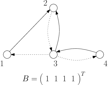
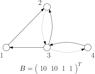
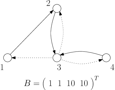
where $w$ is an external disturbance acting on the vehicles. Our problem is to find feedback gains gains $\ell_{ij}\in[0,1]$ that stabilize the formation and minimize the gain from $w$ to $x$ . The problem can be solved by applying Theorem 8 with

$\displaystyle A$	$\displaystyle=\diag\{-1,0,0,-4\}$	$\displaystyle C$	$\displaystyle=\left(\begin{array}[]{rrrr}\!\!1&1&1&1\end{array}\right)$
$\displaystyle E$	$\displaystyle=\left(\begin{array}[]{rrrrrr}\!\!1&0&0&0&0&0\\ 0&1&1&0&0&0\\ 0&0&0&1&1&0\\ 0&0&0&0&0&1\end{array}\right)$	$\displaystyle D$	$\displaystyle=0$
$\displaystyle L$	$\displaystyle=\diag\{\ell_{13},\ell_{21},\ell_{23},\ell_{32},\ell_{34},\ell_{43}\}$
$\displaystyle F$	$\displaystyle=\left(\begin{array}[]{rrrr}\!\!-1&0&1&0\\ 1&-1&0&0\\ 0&-1&1&0\\ 0&1&-1&0\\ 0&0&-1&1\\ 0&0&1&-1\end{array}\right)$	$\displaystyle H$	$\displaystyle=\left(\begin{array}[]{r}\!\!0\\ 0\\ 0\\ 0\\ 0\\ 0\end{array}\right)$

Solutions for three different cases are illustrated in Figure 4.

$\Box$

VI Positively Dominated Systems

So far, the emphasis has been on state space models. However, for many applications input-output models are more natural as a starting point. In this section, we will therefore extend the main ideas of the previous sections to such models. First we need to define a notion of positivity for input-output models. One option would be to work with non-negative impulse responses like in Theorem 3. However, to verify for a given rational transfer function that the impulse response is non-negative has proved to be NP-hard! See [3] for the discrete time problem and [1] for continuous time. Instead we will use the following definition.

$\mathbf{G}\in\mathbb{RH}_{\infty}^{m\times n}$ is called positively dominated if every matrix entry satisfies $|\mathbf{G}_{jk}(i\omega)|\leq\mathbf{G}_{jk}(0)$ for all $\omega\in\mathbb{R}$ . The set of all such matrices is denoted $\mathbb{DH}_{\infty}^{m\times n}$ . The essential scalar frequency inequality can be tested by semi-definite programming, since $|b(i\omega)/a(i\omega)|\leq b(0)/a(0)$ holds for $\omega\in\mathbb{R}$ if and only if the polynomial $|a(i\omega)|^{2}b(0)^{2}-|b(i\omega)|^{2}a(0)^{2}$ can be written as a sum of squares.

Some properties of positively dominated transfer functions follow immediately:

Proposition 9

Let $\mathbf{G},\mathbf{H}\in\mathbb{DH}_{\infty}^{n\times n}$ . Then $\mathbf{G}\mathbf{H}\in\mathbb{DH}_{\infty}^{n\times n}$ and $a\mathbf{G}+b\mathbf{H}\in\mathbb{DH}_{\infty}^{n\times n}$ when $a,b\in\mathbb{R}_{+}$ . Moreover $\|\mathbf{G}\|_{\infty}=\|\mathbf{G}(0)\|$ .

The following property is also fundamental:

Theorem 10

Let $\mathbf{G}\in\mathbb{DH}_{\infty}^{n\times n}$ . Then $(I-\mathbf{G})^{-1}\in\mathbb{DH}_{\infty}^{n\times n}$ if and only if $\mathbf{G}(0)$ is Schur.

Proof. That $(I-\mathbf{G})^{-1}$ is stable and positively dominated implies that $[I-\mathbf{G}(0)]^{-1}$ exists and is nonnegative, so $\mathbf{G}(0)$ must be Schur according to Proposition 2. On the other hand, if $\mathbf{G}(0)$ is Schur we may choose ${\xi}\in\mathbb{R}_{+}$ and $\epsilon>0$ with $\mathbf{G}(0){\xi}<(1-\epsilon){\xi}$ . Then for every $z\in\mathbb{C}^{n}$ with $0<|z|<\xi$ and $s\in\mathbb{C}$ with $\hbox{Re }s\geq 0$ we have

\displaystyle|\mathbf{G}(s)^{t}z|\leq\mathbf{G}(0)^{t}|z|<(1-\epsilon)^{t}|z|

\displaystyle\hbox{for }t=1,2,3,\ldots

Hence $\sum_{k=0}^{\infty}\mathbf{G}(s)^{t}z$ is convergent and bounded above by $\sum_{k=0}^{\infty}\mathbf{G}(0)^{t}|z|=[I-\mathbf{G}(0)]^{-1}|z|$ . The sum of the series solves the equation $[I-\mathbf{G}(s)]\sum_{k=0}^{\infty}\mathbf{G}(s)^{t}z=z$ , so therefore $\sum_{k=0}^{\infty}\mathbf{G}(s)^{t}z=[I-\mathbf{G}(s)]^{-1}z$ . This proves $(I-\mathbf{G})^{-1}$ is stable and positively dominated and the proof is complete. $\Box$

Theorem 8 has the following counterpart for positively dominated systems, as illustrated in Figure 5.

Theorem 11

Let $\mathcal{D}$ be the set of $m\times m$ diagonal matrices with entries in $[0,1]$ , while $\mathbf{B}\in\mathbb{DH}_{\infty}^{n\times k}$ , $\mathbf{C}\in\mathbb{DH}_{\infty}^{l\times n}$ , $\mathbf{D}\in\mathbb{DH}_{\infty}^{l\times k}$ , $\mathbf{E}\in\mathbb{DH}_{\infty}^{n\times m}$ and $\mathbf{F}\in\mathbb{RH}_{\infty}^{m\times n}$ . Suppose $\mathbf{A}+\mathbf{E}L\mathbf{F}\in\mathbb{DH}_{\infty}^{n\times n}$ for all $L\in\mathcal{D}$ .

Then the following two conditions are equivalent:

(11.1)

There is $L\in\mathcal{D}$ with $(I-\mathbf{A}-\mathbf{E}{L}\mathbf{F})^{-1}\in\mathbb{DH}_{\infty}^{n\times n}$ and $\|\mathbf{C}(I-\mathbf{A}-\mathbf{E}L\mathbf{F})^{-1}\mathbf{B}+\mathbf{D}\|_{1-\ind}<\gamma$ .

(11.2)

There exist $p\in\mathbb{R}_{+}^{n}$ , $q\in\mathbb{R}_{+}^{m}$ with

	$\displaystyle\mathbf{A}(0)^{T}p+\mathbf{C}(0)^{T}{\bf 1}+\mathbf{F}(0)^{T}q$	$\displaystyle<p$
	$\displaystyle\mathbf{B}(0)^{T}p+\mathbf{D}(0)^{T}{\bf 1}$	$\displaystyle<\gamma{\bf 1}$
	$\displaystyle\mathbf{E}(0)^{T}p$	$\displaystyle\geq q$

If $p,q$ satisfy (11.2), then (11.1) holds for every $L$ such that $q=L\mathbf{E}(0)^{T}p$ .

Proof. Proposition 9 and Theorem 10 show that (11.1) holds if and only if $\mathbf{A}(0)-\mathbf{E}(0){L}\mathbf{F}(0)$ is Schur and

\displaystyle\|\mathbf{C}[I-\mathbf{A}(0)-\mathbf{E}(0)L\mathbf{F}(0)]^{-1}\mathbf{B}(0)+\mathbf{D}(0)\|_{1-\ind}<\gamma

According to Theorem 6, this is true if and only if there exists $p\in\mathbb{R}_{+}^{n}$ such that

\displaystyle\begin{bmatrix}\mathbf{A}(0)+\mathbf{E}(0)L\mathbf{F}(0)&\mathbf{B}(0)\\ \mathbf{C}(0)&\mathbf{D}(0)\end{bmatrix}^{T}\begin{bmatrix}p\\ {\bf 1}\end{bmatrix}<\begin{bmatrix}p\\ \gamma{\bf 1}\end{bmatrix}.

This is equivalent to (11.2) if we set $q=L\mathbf{E}(0)^{T}{p}$ , so the desired equivalence between (11.1) and (11.2) follows. $\Box$

Example 5. Formation of vehicles with inertia. In Example 3, the inputs and disturbances were supposed to have an immediate impact on the vehicle velocities, i.e. the inertia of the vehicles was neglected. Alternatively, a model that takes the inertia into account can be stated as follows:

\displaystyle\ddot{x}_{i}

\displaystyle=\sum_{j}{}\ell_{ij}(x_{j}-x_{i})+u_{i}+w_{i}

\displaystyle i=1,\ldots,N

where $u_{i}$ is a control force, $w_{i}$ is a disturbance force and ${\ell}_{ij}$ is the spring constant between the vehicles $i$ and $j$ . Suppose that local control laws $u_{i}=-k_{i}x_{i}-d_{i}\dot{x}$ are given and consider the problem to find spring constants ${\ell}_{ij}\in[0,\overline{\ell}_{ij}]$ that minimize the gain from $w_{1}$ to $x_{1}$ .

The closed loop system has the frequency domain description

		$\displaystyle\bigg(s^{2}+d_{i}s+k_{i}+\sum_{j}\overline{\ell}_{ij}\bigg)X_{i}(s)$
		$\displaystyle=\sum_{j}\bigg({\ell}_{ij}X_{j}(s)+(\overline{\ell}_{ij}-{\ell}_{ij})X_{i}(s)\bigg)+W_{i}(s).$

Similarly to Example 3, we write this on matrix form as

\displaystyle X

\displaystyle=(\mathbf{A}+\mathbf{E}L\mathbf{F})X+\mathbf{B}W

The transfer matrices $\mathbf{B}$ , $\mathbf{E}$ and $\mathbf{A}+\mathbf{E}L\mathbf{F}$ are positively dominated for all $L\in\mathcal{D}$ provided that $d_{i}\geq k_{i}+\sum_{j}\overline{\ell}_{ij}$ . Hence Theorem 11 can then be applied to find the optimal spring constants. Notice that $\ell_{ij}$ and $\ell_{ji}$ must be optimized separately, even though by symmetry they must be equal at optimum. $\Box$

VII Scalable Verification of the Lyapunov Inequality

In the preceding sections we have derived scalable conditions for verification of stability and optimality, using generalizations of the linear inequalities in (1.2) and (1.3) of Proposition 1. To address multi-variable systems using linear programming, the natural performance measures have been input-output gains with signals measured $L_{1}$ -norm or $L_{\infty}$ -norm.

A more well-known alternative, used in the classical $H_{\infty}$ control theory, is to measure signals with $L_{2}$ -norm. This was done in [24] using generalizations of condition (1.4), however without discussion of scalability aspects. The purpose of the next theorem is to show that for positive systems also verification of semi-definite inequalities, like the Lyapunov inequality $A^{T}P+PA\prec 0$ , can be decomposed into tests that scale linearly with the number of non-zero matrix entries.

Theorem 12

A symmetric Metzler matrix with $m$ non-zero entries above the diagonal is negative semi-definite if and only if it can be written as a sum of $m$ negative semi-definite matrices, each of which has only four non-zero entries.

The proof of Theorem 12 will be based on the following minor modification of [12, Theorem 3.1]:

Proposition 13 (Positive Quadratic Programming)

Suppose $M_{0},\ldots,M_{K}$ are Metzler and $b_{1},\ldots,b_{K}\in\mathbb{R}$ . Then

\displaystyle\begin{array}[]{llcll}\max&x^{T}M_{0}x&=&\max&\trace(M_{0}X)\\[2.84526pt] x\in\mathbb{R}^{n}_{+}&x^{T}M_{k}x\,\geq\,b_{k}&&X\succeq 0&\trace(M_{k}X)\geq b_{k}\\ &k=1,\ldots,K&&&k=1,\ldots,K\end{array}

The value on the right hand side remains the same if the condition $X\succeq 0$ is relaxed to $X\in\mathbb{X}$ , where $\mathbb{X}$ is the set of symmetric matrices $(x_{ij})\in\mathbb{R}^{n\times n}$ satisfying $x_{ii}\geq 0$ and $x_{ij}^{2}\leq x_{ii}x_{jj}$ for all $i,j$ . Moreover, if there exists a matrix $X$ in the interior of $\mathbb{X}$ with $\trace(M_{k}X)\geq b_{k}$ for every $k$ , then the maximum of (13) is equal to the minimum of $-\sum_{k}\tau_{k}b_{k}$ over $\tau_{1},\ldots,\tau_{K}\geq 0$ such that $M_{0}+\sum_{k}\tau_{k}M_{k}\preceq 0$ .

Remark 7. The problem on the right of (13) is always convex and readily solvable by semidefinite programming. The problem on the left is generally not a convex program, since the matrices $M_{k}$ may be indefinite. However, the maximization on the left is concave in $(x_{1}^{2},\ldots,x_{n}^{2})$ [17]. This is because every product $x_{i}x_{j}$ is the geometric mean of two such variables, hence concave [4, p. 74].

Remark 8. The second statement of Proposition 13 is important for scalability, since the condition $X\in\mathbb{X}$ has a natural decomposition and only entries of $X$ that correspond to non-zero entries of $M_{k}$ need to be taken into account.

Proof of Proposition 13. Every $x$ satisfying the constraints on the left hand side of (13) corresponds to a matrix $X=xx^{T}$ satisfying the constraints on the right hand side. This shows that the right hand side of (13) is at least as big as the left.

On the other hand, let $X=(x_{ij})$ be a positive definite matrix. In particular, the diagonal elements $x_{11},\ldots,x_{nn}$ are non-negative and $x_{ij}\leq\sqrt{x_{ii}x_{jj}}$ . Let $x=(\sqrt{x_{11}},\ldots,\sqrt{x_{nn}})$ . Then the matrix $xx^{T}$ has the same diagonal elements as $X$ , but has off-diagonal elements $\sqrt{x_{ii}x_{jj}}$ instead of $x_{ij}$ . The fact that $xx^{T}$ has off-diagonal elements at least as big as those of $X$ , together with the assumption that the matrices $M_{k}$ are Metzler, gives $x^{T}M_{k}x\geq\trace(M_{k}X)$ for $k=1,\ldots,K$ . This shows that the left hand side of (13) is at least as big as the right. Nothing changes if $X$ is not positive definite but $X\in\mathbb{X}$ , so the second statement is also proved.

For the last statement, note that the conditions $\trace(M_{k}X)\geq b_{k}$ are linear in $X$ , so strong duality holds [22, Theorem 28.2] and the right hand side of (13) has a finite maximum if and only if $M_{0}+\sum_{k=1}^{K}\tau_{k}M_{k}\preceq 0$ for some $\tau_{1},\ldots,\tau_{K}\geq 0$ . $\Box$

Proof of Theorem 12. Let $\mathcal{E}$ be the set of indices $(k,l)$ of non-zero off-diagonal entries in $M$ . Define

\displaystyle\mathbb{X}_{\mathcal{E}}

\displaystyle=\left\{X\in\mathbb{R}^{n\times n}:\,\,\hbox{$[e_{k}\;\;e_{l}]^{T}X[e_{k}\;\;e_{l}]\succeq 0$ for all }(k,l)\in\mathcal{E}\right\}

where $e_{1},\ldots,e_{n}$ are the unit vectors in $\mathbb{R}^{n}$ . If $M$ is negative semi-definite, then

	$\displaystyle 0$	$\displaystyle=\max_{\|x\|\leq 1}x^{T}Mx=\max_{X\in\mathbb{X}_{\mathcal{E}}}\trace(MX)$
		$\displaystyle=\min_{N_{kl}\succeq 0}\max_{X\in\mathbb{R}^{n\times n}}\trace(MX)+\!\!\!\!\sum_{(k,l)\in\mathcal{E}}\!\!\trace\left(N_{kl}[e_{k}\;\;e_{l}]^{T}X[e_{k}\;\;e_{l}]\right)$
		$\displaystyle=\min_{N_{kl}\succeq 0}\max_{X\in\mathbb{R}^{n\times n}}\trace\left[\left(M+\sum_{(k,l)\in\mathcal{E}}[e_{k}\;\;e_{l}]N_{kl}[e_{k}\;\;e_{l}]^{T}\right)X\right]$

where $N_{kl}\in\mathbb{R}^{2\times 2}$ for every $k$ and $l$ . In particular, there exists a choice of the matrices $N_{kl}$ that makes $M+\sum_{(k,l)\in\mathcal{E}}[e_{k}\;\;e_{l}]N_{kl}[e_{k}\;\;e_{l}]^{T}=0$ . This completes the proof. $\Box$

VIII The KYP Lemma for Positive Systems

Input-output gain is certainly not the only way to quantify the performance of a linear time-invariant system. A more general class of specifications known as Integral Quadratic Constraints [18] can be tested using the Kalman-Yakubovich-Popov lemma. It is therefore of interest to see that the corresponding result of [24] for positive systems can be generalized the following way:

Theorem 14

Let $A\in\mathbb{R}^{n\times n}$ be Metzler and Hurwitz, while $B\in\mathbb{R}_{+}^{n\times m}$ and the pair $(-A,B)$ is stabilizable. Suppose that all entries of $Q\in\mathbb{R}^{(n+m)\times(n+m)}$ are nonnegative, except for the last $m$ diagonal elements. Then the following statements are equivalent:

(14.1)

For $\omega\in[0,\infty]$ is is true that

\displaystyle\begin{bmatrix}(i\omega I-A)^{-1}B\\ I\end{bmatrix}^{*}Q\begin{bmatrix}(i\omega I-A)^{-1}B\\ I\end{bmatrix}\preceq 0

(14.2)

$\quad\begin{bmatrix}-A^{-1}B\\ I\end{bmatrix}^{T}Q\begin{bmatrix}-A^{-1}B\\ I\end{bmatrix}\preceq 0$ .

(14.3)

There exists a diagonal $P\succeq 0$ such that

\displaystyle Q+\begin{bmatrix}A^{T}P+PA&PB\\ B^{T}P&0\end{bmatrix}\preceq 0

(14.4)

There exist $x,p\in\mathbb{R}^{n}_{+}$ , $u\in\mathbb{R}^{m}_{+}$ with $Ax+Bu\leq 0$ ,

Q\begin{bmatrix}x\\ u\end{bmatrix}+\begin{bmatrix}A^{T}\\ B^{T}\end{bmatrix}p\leq 0

Moreover, if all inequalities are replaced by strict ones, then the equivalences hold even without the stabilizability assumption.

Remark 9. For $A=-1$ , $B=0$ , $Q=$ $\begin{bmatrix}0&1\\ 1&0\end{bmatrix}$ , condition (14.1) holds, but not (14.3). This demonstrates that the stabilizability of $(-A,B)$ is essential.

Remark 10. Our statement of the KYP lemma for continuous and discrete time positive systems extends earlier versions of [24, 19] in several respects: Non-strict inequality, more general $Q$ and a fourth equivalent condition in terms of linear programming rather than semi-definite programming.

Proof. One at a time, we will prove the implications (14.1) $\Rightarrow$ (14.2) $\Rightarrow$ (14.3) $\Rightarrow$ (14.1) and (14.2) $\Leftrightarrow$ (14.4). Putting $\omega=0$ immediately gives (14.2) from (14.1).

Assume that (14.2) holds. The matrix $-A^{-1}$ is nonnegative, so $\begin{bmatrix}x\\ w\end{bmatrix}^{T}$ $Q\,$ $\begin{bmatrix}x\\ w\end{bmatrix}$ $\leq 0$ for all $x\in\mathbb{R}^{n}_{+}$ , $w\in\mathbb{R}_{+}^{m}$ with

\displaystyle x

\displaystyle\leq-A^{-1}Bw

(20)

The inequality (20) follows (by multiplication with $-A^{-1}$ from the left) from the constraint $0\leq Ax+Bw$ , which can also be written $0\leq A_{i}x+B_{i}w$ for $i=1,\ldots,n$ , where $A_{i}$ and $B_{i}$ denote the $i$ :th rows of $A$ and $B$ respectively. For non-negative $x$ and $w$ , this is equivalent to

\displaystyle 0

\displaystyle\leq x_{i}(A_{i}x+B_{i}w)

\displaystyle i

\displaystyle=1,\ldots,n

(21)

Hence (14.2) implies $\begin{bmatrix}x\\ w\end{bmatrix}^{T}$ $Q\,$ $\begin{bmatrix}x\\ w\end{bmatrix}$ $\leq 0$ for $x\in\mathbb{R}^{n}_{+}$ , $w\in\mathbb{R}_{+}^{m}$ satisfying (21). Proposition 13 will next be used to verify existence of $\tau_{1},\ldots,\tau_{n}\geq 0$ such that the quadratic form

\displaystyle\sigma(x,w)=\Biggl[\!\!\begin{array}[]{c}x\\ w\end{array}\!\!\Biggr]^{T}Q\Biggl[\!\!\begin{array}[]{c}x\\ w\end{array}\!\!\Biggr]+\sum_{i}\tau_{i}x_{i}(A_{i}x+B_{i}w)

is negative semi-definite. However, the application of Proposition 13 requires existence of a positive definite $X$ such that all diagonal elements of

\displaystyle\begin{bmatrix}A&B\end{bmatrix}X\begin{bmatrix}I\\ 0\end{bmatrix}

are positive. The pair $(-A,B)$ is stabilizable, so there exists $K$ that make all eigenvalues of $A+BK$ unstable and therefore $(A+BK)Z+Z(A+BK)^{T}=I$ has a symmetric positive definite solution $Z$ . Hence the desired $X$ can be constructed as

\displaystyle X=\begin{bmatrix}Z&ZK^{T}\\ KZ&*\end{bmatrix}

where the lower right corner is chosen big enough to make $X\succ 0$ .

Define $P=\diag(\tau_{1},\ldots,\tau_{n})\succeq 0$ . Then $\sigma$ being negative definite means that

\displaystyle Q+\begin{bmatrix}A^{T}P+PA&PB\\ B^{T}P&0\end{bmatrix}\preceq 0

so (14.3) follows.

Assume that (14.3) holds. Integrating $\sigma(x(t),w(t))$ over time gives

\displaystyle 0

\displaystyle\geq\int_{0}^{\infty}\left(\Biggl[\!\!\begin{array}[]{c}x\\ w\end{array}\!\!\Biggr]^{T}Q\Biggl[\!\!\begin{array}[]{c}x\\ w\end{array}\!\!\Biggr]+x^{T}P(Ax+Bw)\right)dt

For square integrable solutions to $\dot{x}=Ax+Bw$ , $x(0)=0$ we get

	$\displaystyle 0$	$\displaystyle\geq\int_{0}^{\infty}\left(\Biggl[\!\!\begin{array}[]{c}x\\ w\end{array}\!\!\Biggr]^{T}Q\Biggl[\!\!\begin{array}[]{c}x\\ w\end{array}\!\!\Biggr]+\frac{d}{dt}(x^{T}Px/2)\right)dt$
		$\displaystyle=\int_{0}^{\infty}\Biggl[\!\!\begin{array}[]{c}x(t)\\ w(t)\end{array}\!\!\Biggr]^{T}Q\Biggl[\!\!\begin{array}[]{c}x(t)\\ w(t)\end{array}\!\!\Biggr]dt$

which in frequency domain implies (14.1). Hence (14.1) $\Rightarrow$ (14.2) $\Rightarrow$ (14.3) $\Rightarrow$ (14.1).

Assuming again (14.2) gives, by Proposition 1, existence of $u\in\mathbb{R}^{m}_{+}$ such that

\displaystyle\left(\begin{bmatrix}-A^{-1}B\\ I\end{bmatrix}^{T}Q\begin{bmatrix}-A^{-1}B\\ I\end{bmatrix}\right)u\leq 0

Setting $x=-A^{-1}u$ gives $x\in\mathbb{R}^{n}_{+}$ and

\displaystyle\begin{bmatrix}-A^{-1}&A^{-1}B\\ 0&-I\end{bmatrix}^{T}Q\begin{bmatrix}x\\ u\end{bmatrix}\geq 0

due to the sign structure of $Q$ . Let $\begin{bmatrix}p^{T}&q^{T}\end{bmatrix}^{T}$ be the column on the left hand side. Multiplying with $\begin{bmatrix}A&B\\ 0&I\end{bmatrix}^{T}$ from the left gives

\displaystyle\begin{bmatrix}A^{T}&0\\ B^{T}&I\end{bmatrix}\begin{bmatrix}p\\ q\end{bmatrix}=-Q\begin{bmatrix}x\\ u\end{bmatrix}

and (14.4) follows.

Finally, suppose that (14.4) holds. Then $x\geq-A^{-1}Bu$ . Multiplying the main inequality from the left with $\begin{bmatrix}-B^{T}A^{-T}&I\end{bmatrix}$ gives

\displaystyle 0

\displaystyle\geq\begin{bmatrix}-A^{-1}B\\ I\end{bmatrix}^{T}Q\begin{bmatrix}x\\ u\end{bmatrix}=\left(\begin{bmatrix}-A^{-1}B\\ I\end{bmatrix}^{T}Q\begin{bmatrix}-A^{-1}B\\ I\end{bmatrix}\right)u

and (14.2) follows.

For strict inequalities, the proofs that (14.2) $\Leftrightarrow$ (14.4) and (14.3) $\Rightarrow$ (14.1) $\Rightarrow$ (14.2) remain the same. Assuming that (14.2) holds with strict inequality, we get

\displaystyle\begin{bmatrix}-A^{-1}B\\ I\end{bmatrix}^{*}(Q+\epsilon I)\begin{bmatrix}-A^{-1}B\\ I\end{bmatrix}\preceq 0

for some scalar $\epsilon>0$ . Hence, there exists a diagonal $P\succeq 0$ such that

\displaystyle Q+\epsilon I+\begin{bmatrix}A^{T}P+PA&PB\\ B^{T}P&0\end{bmatrix}\preceq 0

Adding a small multiple of the identity to $P$ gives $P\succ 0$ such that

\displaystyle Q+\begin{bmatrix}A^{T}P+PA&PB\\ B^{T}P&0\end{bmatrix}\prec 0

so also (14.3) holds with strict inequality. Hence the proof is complete. $\Box$

An analogous discrete time result is stated here and proved in the appendix:

Theorem 15

Let $A\in\mathbb{R}_{+}^{n\times n}$ be Schur, while $B\in\mathbb{R}_{+}^{n\times m}$ and the pair $(A,B)$ is anti-stabilizable. Suppose that all entries of $Q\in\mathbb{R}^{(n+m)\times(n+m)}$ are nonnegative, except for the last $m$ diagonal elements. Then the following statements are equivalent:

(15.1)

For $\omega\in[0,\infty]$ is is true that

\displaystyle\begin{bmatrix}(e^{i\omega}I-A)^{-1}B\\ I\end{bmatrix}^{*}Q\begin{bmatrix}(e^{i\omega}I-A)^{-1}B\\ I\end{bmatrix}\preceq 0

(15.2)

$\quad\begin{bmatrix}(I-A)^{-1}B\\ I\end{bmatrix}^{*}Q\begin{bmatrix}(I-A)^{-1}B\\ I\end{bmatrix}\preceq 0$ .

(15.3)

There exists a diagonal $P\succeq 0$ such that

\displaystyle Q+\begin{bmatrix}A^{T}PA-P&A^{T}PB\\ B^{T}PA&B^{T}PB\end{bmatrix}\preceq 0

(15.4)

There are $x,p\in\mathbb{R}^{n}_{+}$ , $u\in\mathbb{R}^{m}_{+}$ with $x\geq Ax+Bu$ ,

Q\begin{bmatrix}x\\ u\end{bmatrix}+\begin{bmatrix}A^{T}-I\\ B^{T}\end{bmatrix}p\leq 0

Moreover, if all inequalities are taken to be strict, then the equivalences hold even without the anti-stabilizability assumption.

Proof. The theorem can be proved in analogy with the proof of Theorem 14. Alternatively, it can be derived from Theorem 14 using a bilinear transformation in the following way:

Instead of $e^{i\omega}$ , one can parametrize the unit circle as $\frac{1+i\omega}{1-i\omega}$ . Hence (15.1) is equivalent to saying that

\displaystyle\begin{bmatrix}x\\ u\end{bmatrix}^{*}Q\begin{bmatrix}x\\ u\end{bmatrix}\leq 0

for all solutions $(\omega,x,u)$ to the equation $\left(\frac{1+i\omega}{1-i\omega}I-A\right)x=Bu$ . Alternatively, introducing

	$\displaystyle\widehat{A}$	$\displaystyle=(A-I)(A+I)^{-1}$
	$\displaystyle\widehat{B}$	$\displaystyle=2(A+I)^{-1}B$
	$\displaystyle\widehat{x}$	$\displaystyle=x+Ax+Bu$
	$\displaystyle S$	$\displaystyle=\begin{bmatrix}(A+I)^{-1}&-(A+I)^{-1}B\\ 0&I\end{bmatrix}$
	$\displaystyle\widehat{Q}$	$\displaystyle=S^{T}QS$

the condition can be re-written as the statement that

\displaystyle\begin{bmatrix}\widehat{x}\\ u\end{bmatrix}^{*}\widehat{Q}\begin{bmatrix}\widehat{x}\\ u\end{bmatrix}\leq 0

for all solutions $(\omega,\widehat{x},\widehat{u})$ to the equation $(i\omega I-\widehat{A})\widehat{x}=\widehat{B}u$ . According to Theorem 14, this is equivalent to validity of the inequality for $\omega=0$ , i.e. (15.2). It is also equivalent to existence of a diagonal $P\succeq 0$ such that

\displaystyle\widehat{Q}+\begin{bmatrix}\widehat{A}^{T}P+P\widehat{A}&P\widehat{B}\\ \widehat{B}^{T}P&0\end{bmatrix}\preceq 0

Multiplying by $\begin{bmatrix}A+I&B\\ 0&I\end{bmatrix}$ from the right and its transpose from the left, the matrix inequality (after trivial manipulations) becomes

\displaystyle Q+2\begin{bmatrix}A^{T}PA-P&A^{T}PB\\ B^{T}PA&B^{T}PB\end{bmatrix}\preceq 0

Replacing $2P$ by $P$ gives equivalence to (15.3). Also by Theorem 14, it is equivalent to existence of $\widehat{x},p\in\mathbb{R}^{n}_{+}$ , $\widehat{u}\in\mathbb{R}^{m}_{+}$ such that

\displaystyle\widehat{Q}\begin{bmatrix}\widehat{x}\\ u\end{bmatrix}+\begin{bmatrix}\widehat{A}^{T}\\ \widehat{B}^{T}\end{bmatrix}p\leq 0

Left multiplication by $S^{-T}$ and substitution $(x,u)=S(\widehat{x},u)$ gives equivalence to (15.4). $\Box$

As an application of the equivalence between (14.1) and (14.2), we consider an example devoted to optimal power flow in an electrical network, a time-varying version of a problem considered in[13]:

Example 6. Optimal power flow in an electrical network.

Consider a power transmission network as in Figure 6. The current from node $j$ to node $k$ is governed by the voltage difference $v_{j}-v_{k}$ according to the differential equation

\displaystyle L_{jk}\frac{di_{jk}}{dt}

\displaystyle=-R_{jk}i_{jk}+v_{j}(t)-v_{k}(t)

(22)

and the external currents are determined by Kirchoff’s law

\displaystyle\begin{cases}i_{1}(t)=-i_{41}(t)-i_{21}(t)\\ i_{2}(t)=i_{21}(t)-i_{32}(t)-i_{42}(t)\\ i_{3}(t)=i_{32}(t)\\ i_{4}(t)=i_{41}(t)+i_{42}(t)\end{cases}

(23)

The generation and consumption of power is subject to constraints of the form

\displaystyle\frac{1}{T}\int_{0}^{T}i_{k}(t)v_{k}(t)dt\leq\overline{p}_{k}

(24)

If $k$ is a generator node, then $\overline{p}_{k}>0$ indicates production capacity. Similarly, for loads $\overline{p}_{k}<0$ represents power demand. Transmission lines have capacity constraints of the form

\displaystyle\frac{1}{T}\int_{0}^{T}|v_{k}(t)-v_{j}(t)|^{2}dt\leq c_{kj}

(25)

Finally, the voltages are non-negative and subject to magnitude bounds

\displaystyle\underline{v}_{k}^{2}\leq\frac{1}{T}\int_{0}^{T}v_{k}(t)^{2}dt\leq\overline{v}_{k}^{2}

(26)

We are now interested to minimize the resistive power losses in the network subject to the given constraints:

\displaystyle\begin{cases}\hbox{Minimize }\frac{1}{T}\sum_{k=1}^{4}\int_{0}^{T}i_{k}(t)v_{k}(t)dt\\[5.69054pt] \hbox{subject to }(\ref{eqn:inductive})-(\ref{eqn:magnitude})\end{cases}

Using the theory above, our goal is to prove that minimal losses can be attained with constant voltages and currents.

With line currents being states and voltage differences being inputs, this is a problem of the form

\displaystyle\begin{cases}\hbox{Maximize $\int_{0}^{T}$ {\scriptsize$\begin{bmatrix}x\\ u\end{bmatrix}^{*}$} $Q_{0}$ {\scriptsize$\begin{bmatrix}x\\ u\end{bmatrix}$} $dt$}\\[5.69054pt] \hbox{subject to }\dot{x}(t)=Ax(t)+Bu(t)\\[5.69054pt] \hbox{and $\int_{0}^{T}$ {\scriptsize$\begin{bmatrix}x\\ u\end{bmatrix}^{*}$} $Q_{k}$ {\scriptsize$\begin{bmatrix}x\\ u\end{bmatrix}$} $dt\leq q_{k},\quad k=1,\ldots,m$ }\end{cases}

(27)

where $A\in\mathbb{R}^{n\times n}$ is Metzler and Hurwitz, $B\in\mathbb{R}_{+}^{n\times m}$ and all entries of $Q_{k}\in\mathbb{R}^{(n+m)\times(n+m)}$ are nonnegative except possibly for the last $m$ diagonal elements. To bring the problem on a form where Theorem 14 can be applied, we will apply relaxation in two different ways: The inequalities are handled using Lagrange relaxation and the time interval is extended to $[0,\infty]$ . This brings the problem to the dual form

\displaystyle\begin{cases}\hbox{Minimize }-\sum_{k=1}^{m}\tau_{k}q_{k}\hbox{ subject to $\tau_{k}\geq 0$ such that}\\[5.69054pt] \hbox{$\int_{0}^{\infty}$ {\scriptsize$\begin{bmatrix}x\\ u\end{bmatrix}^{*}$} $(Q_{0}+\sum_{k}\tau_{k}Q_{k})$ {\scriptsize$\begin{bmatrix}x\\ u\end{bmatrix}$} $dt\leq 0$}\\[5.69054pt] \hbox{for all solutions to }\dot{x}(t)=Ax(t)+Bu(t).\end{cases}

In frequency domain, this is written as

\displaystyle\begin{cases}\hbox{Minimize }\sum_{k=1}^{m}\tau_{k}q_{k}\hbox{ subject to $\tau_{k}\geq 0$ and}\\[5.69054pt] \hbox{\small$\begin{bmatrix}(i\omega I-A)^{-1}B\\ I\end{bmatrix}^{*}(Q_{0}+\sum_{k}\tau_{k}Q_{k})\begin{bmatrix}(i\omega I-A)^{-1}B\\ I\end{bmatrix}\preceq 0$}\end{cases}

The equivalence between (14.1) and (14.2) in Theorem 14 shows that the bottleneck is always the frequency $\omega=0$ , so the problem takes the form

\displaystyle\min_{\tau_{k}\geq 0}\sum_{k=1}^{m}\tau_{k}q_{k}\hbox{ subject to }M_{0}+\sum_{k}\tau_{k}M_{k}\preceq 0

where

\displaystyle M_{k}

\displaystyle=\begin{bmatrix}-A^{-1}B\\ I\end{bmatrix}^{*}Q_{k}\begin{bmatrix}-A^{-1}B\\ I\end{bmatrix},

\displaystyle k

\displaystyle=1,\ldots,m

are all Metzler. By Proposition 13 this can be restated as

\displaystyle\max_{u}u^{T}M_{0}u\hbox{ subject to }u^{T}M_{k}u\leq q_{k}

or equivalently

\displaystyle\begin{cases}\hbox{Maximize {\scriptsize$\begin{bmatrix}x\\ u\end{bmatrix}^{T}$} $Q_{0}$ {\scriptsize$\begin{bmatrix}x\\ u\end{bmatrix}$}}\\[5.69054pt] \hbox{subject to }Ax+Bu=0\\[5.69054pt] \hbox{and {\scriptsize$\begin{bmatrix}x\\ u\end{bmatrix}^{T}$} $Q_{k}$ {\scriptsize$\begin{bmatrix}x\\ u\end{bmatrix}$} $\leq q_{k}\quad k=1,\ldots,m$}\end{cases}

(28)

Notice that (28) was obtained from (27) by relaxation, so the optimal value of (28) must be at least as good as the value of (27). At the same time, (28) is the special case of (27) obtained with constant values of the variables, so our goal has been achieved: Minimal losses can be attained with constant voltages and currents. $\Box$

IX Conclusions

The results above demonstrate that the monotonicity properties of positive systems and positively dominated systems bring remarkable benefits to control theory. Most important is the opportunity for scalable verification and synthesis of distributed control systems with optimal input-output performance. In particular, linear programming solutions come with certificates that enable distributed and scalable verification of global optimality, without access to a global model anywhere.

Many important problems remain open for future research. Here are two examples:

•

How can the scalable methods for verification and synthesis be extended to monotone nonlinear systems?
•

How can the controller optimization be extended to scalable methods for optimization of dynamic controllers?

X Acknowledgments

The author is grateful for suggestions and comments by numerous colleagues, including the anonymous reviewers. In particular, Theorem 3 was updated based on suggestions by Andrej Ghulchak and Figure 4 was drawn by Enrico Lovisari. The work has been supported by the Swedish Research Council through the Linnaeus Center LCCC.

References

[1] Paul C. Bell, Jean-Charles Delvenne, Raphaël M. Jungers, and Vincent D. Blondel. The continuous Skolem-Pisot problem. Theoretical Computer Science, 411:3625–3634, 2010.
[2] Abraham Berman and Robert J. Plemmons. Nonnegative matrices in the mathematical sciences. Classics in Applied Mathematics. SIAM, 1994.
[3] Vincent D. Blondel and Natacha Portier. The presence of a zero in an integer linear recurrent sequence is NP-hard to decide. Linear Algebra and its Applications, 351–352:91–98, 2002.
[4] Stephen Boyd and Lieven Vandenberghe. Convex Optimization. Cambridge University Press, 2004.
[5] Corentin Briat. Robust stability and stabilization of uncertain linear positive systems via integral linear constraints: $l_{1}$ -gain and $l_{\infty}$ -gain characterization. International Journal of Robust and Nonlinear Control, 23:1932–1954, 2013.
[6] Lorenzo Farina and Sergio Rinaldi. Positive Linear Systems: Theory and Applications. Wiley, 2000.
[7] M. W. Hirsch. Differential equations and convergence almost everywhere in strongly monotone flows. In Contemporary Mathematics, volume 17, pages 267–285. Amer. Math. Soc., Providence, RI, 1983.
[8] M.W. Hirsch and Hal Smith. Monotone dynamical systems. In Handbook of Differential Equations: Ordinary Differential Equations, volume 2, chapter 4, pages 239–357. Elsevier, 2006.
[9] L. Hörmander. The analysis of linear partial differential operators I. Springer Verlag, 1985.
[10] John A. Jacquez. Compartmental Analysis in Biology and Medicine. BioMedware, 3rd edition, 1996.
[11] Tadeusz Kaczorek. Positive 1D and 2D systems. Springer, 2002.
[12] Sunyoung Kim and Masakazu Kojima. Exact solutions of some nonconvex quadratic optimization problems via SDP and SOCP relaxations. Computational Optimization and Applications, 26:143–154, 2003.
[13] Javad Lavaei, Anders Rantzer, and Steven Low. Power flow optimization using positive quadratic programming. In 18th IFAC World Congress, Milano, Italy, August 2011.
[14] Patrick De Leenheer and Dirk Aeyels. Stabilization of positive linear systems. Systems & Control Letters, 44(4):259–271, November 2001.
[15] Wassily W. Leontief, editor. Input-Output Economics. Oxford University Press, New York, 2nd edition, 1986.
[16] David G. Luenberger. Introduction to dynamic systems: Theory, models, and applications. Wiley (New York), 1979.
[17] A. Megretski, 2010. Personal Communication.
[18] Alexander Megretski and Anders Rantzer. System analysis via Integral Quadratic Constraints. IEEE Transactions on Automatic Control, 42(6):819–830, June 1997.
[19] Federico Najson. On the Kalman-Yakubovich-Popov lemma for discrete-time positive systems: A novel simple proof and some related results. International Journal of Control, 86(10):1813–1823, 2013.
[20] Ait Rami. Solvability of static output-feedback stabilization for LTI positive systems. Systems & Control Letters, 60:704–708, 2011.
[21] M. Ait Rami and F. Tadeo. Controller synthesis for positive linear systems with bounded controls. IEEE Transactions on Circuits and Systems II: Express Briefs, 54(2):151–155, 2007.
[22] R. Tyrrell Rockafellar. Convex Analysis. Princeton Landmarks in Mathematics and Physics. Princeton University Press, 1997.
[23] E. Seneta. Non-negative Matrices and Markov Chains. Springer Series in Statistics. Springer, New York, 2nd edition, 1981.
[24] Takashi Tanaka and Cédric Langbort. The bounded real lemma for internally positive systems and H-infinity structured static state feedback. IEEE Transactions on Automatic Control, 56(9):2218–2223, September 2011.
[25] J.C. Willems. Lyapunov functions for diagonally dominant systems. Automatica, pages 519–523, 1976.

	$\displaystyle\\|y\\|_{1}$	$\displaystyle=\sum_{k}\int_{0}^{\infty}\bigg\|\sum_{l}\int_{0}^{t}g_{kl}(t-\tau)w_{l}(\tau)d\tau\bigg\|_{1}dt$
		$\displaystyle\leq\sum_{k}\int_{0}^{\infty}\sum_{l}\int_{0}^{t}g_{kl}(t-\tau)\|w_{l}(\tau)\|d\tau dt$
		$\displaystyle=\sum_{k,l}\int_{0}^{\infty}\bigg(\int_{\tau}^{\infty}g_{kl}(t-\tau)dt\bigg)\|w_{l}(\tau)\big\|d\tau$
		$\displaystyle=\sum_{k,l}\left(\int_{0}^{\infty}g_{kl}(t)dt\right)\\|w_{l}\\|_{1}$
		$\displaystyle=\sum_{k,l}\mathbf{G}_{kl}(0)\\|w_{l}\\|_{1}$
		$\displaystyle\leq\max_{l}\left(\sum_{k}\mathbf{G}_{kl}(0)\right)\\|w\\|_{1}$
		$\displaystyle=\\|\mathbf{G}(0)\\|_{1-\ind}\cdot\\|w\\|_{1}$

	$\displaystyle\\|y\\|_{\infty}$	$\displaystyle=\max_{k,t}\left\|\sum_{l}\int_{0}^{\infty}g_{kl}(\tau)w_{l}(t-\tau)d\tau\right\|$
		$\displaystyle\leq\max_{k}\left(\sum_{l}\int_{0}^{\infty}g_{kl}(\tau)d\tau\right)\\|w\\|_{\infty}$
		$\displaystyle=\max_{k}\left(\sum_{l}\mathbf{G}_{kl}(0)\right)\\|w\\|_{\infty}$
		$\displaystyle=\\|\mathbf{G}(0)\\|_{\infty-\ind}\cdot\\|w\\|_{\infty}$