Calculating principal eigen-functions of non-negative integral kernels: particle approximations and applications

Nick Whiteley ^†^†thanks: School of Mathematics, University of Bristol, University Walk, Bristol, BS8 1TW. Nikolas Kantas ^†^†thanks: Department of Mathematics, Imperial College London, South Kensington Campus, London SW7 2AZ.

Abstract

Often in applications such as rare events estimation or optimal control it is required that one calculates the principal eigen-function and eigen-value of a non-negative integral kernel. Except in the finite-dimensional case, usually neither the principal eigen-function nor the eigen-value can be computed exactly. In this paper, we develop numerical approximations for these quantities. We show how a generic interacting particle algorithm can be used to deliver numerical approximations of the eigen-quantities and the associated so-called “twisted” Markov kernel as well as how these approximations are relevant to the aforementioned applications. In addition, we study a collection of random integral operators underlying the algorithm, address some of their mean and path-wise properties, and obtain $L_{r}$ error estimates. Finally, numerical examples are provided in the context of importance sampling for computing tail probabilities of Markov chains and computing value functions for a class of stochastic optimal control problems.

Keywords: interacting particle methods, eigen-functions, rare events estimation, optimal control, diffusion Monte Carlo

1 Introduction

On a state space $\mathsf{X}$ consider a bounded function $G:\mathsf{X}\rightarrow\mathbb{R}_{+}$ , a Markov probability kernel $M$ . The central object of interest in this paper is the integral kernel $Q$ given by

Q(x,dx^{\prime}):=G(x)M(x,dx^{\prime}).

Under some regularity assumptions, $Q$ has an isolated, real, maximal eigen-value $\lambda_{\star}$ , with which is associated a positive (right) eigen-function $h_{\star}$ ,

Q(h_{\star})=\lambda_{\star}h_{\star},

(1)

where for a function $\varphi$ on $\mathsf{X}$ , we write $Q(\varphi)(x):=\int Q(x,dx^{\prime})\varphi(x^{\prime})$ . When $\mathsf{X}$ is finite set, $\lambda_{\star}$ is the Perron-Frobenius eigen-value and $h_{\star}$ the right eigen-vector. In this paper we are interested in the case where $\mathsf{X}$ is a general space, so not necessarily finite or countable. In general state spaces an extended Perron-Frobenius theory applies, (see Nummelin (2004) for an account), but in most cases $\lambda_{\star},h_{\star}$ cannot be determined analytically, so numerical approximations are required and this is what this paper aims to address.

Treatment of the existence of $\lambda_{\star}$ and $h_{\star}$ outside of settings in which $\mathsf{X}$ is a finite set dates at least as far as (Kolmogorov, 1938; Yaglom, 1947; Harris, 1963), where $Q$ arose as a conditional moment measure associated with a branching process; see Collet et al. (2012) for a modern perspective in the context of quasi-stationary distributions and stochastic processes conditioned on long-term survival. In addition, $Q$ and $h_{\star}$ have often appeared as critical quantities in various more recent applications. In statistical mechanics $Q$ corresponds to the Hamiltonian and $h_{\star}$ could be viewed as the Schrödinger ground energy state for molecules, e.g. (Rousset, 2006; Makrini et al., 2007). Similarly, in particle physics $Q\bigl(1\bigr)\left(x\right)$ can be used to model the one-step probability of survival of of a particle moving in an absorbing medium (Del Moral, 2013, Chapter 7), (Del Moral and Doucet, 2004). In stochastic optimal control, $Q$ arises naturally as a multiplicative Bellman or Dynamic Programming operator in discrete time problems when a Kullback-Leibler divergence term is used in the stage cost (Albertini and Runggaldier, 1988; Todorov, 2008; Dvijotham and Todorov, 2011) or in particular continuous time models with affine dynamics in the control and additive costs that are quadratic to the control input; see (Fleming, 1982; Sheu, 1984) or (Todorov, 2008; Theodorou et al., 2010; Kappen, 2005) for more details. In these specific control problems, $h_{\star}$ can be viewed as a logarithmic transformation of the value function. Finally, $h_{\star}$ appears in the large deviations theory of Markov chains, see for example (Ney and Nummelin, 1987); if $(X_{n};n\geq 0)$ is a Markov chain with transition kernel $M$ , initialized from $X_{0}=x$ , $U$ an appropriate function and $G(x):=e^{\alpha U(x)}$ for a particular value of $\alpha,$ then it is only and explicitly through $h_{\star}(x)$ that the initial condition enters Bahadur-Rao-type asymptotics associated with partial sums $\sum_{p=0}^{n-1}U(X_{p})$ (Kontoyiannis and Meyn, 2003).

A related object of interest in many applications of interest is the “twisted” Markov kernel:

P_{\star}(x,dx^{\prime}):=\frac{Q(x,dx^{\prime})h_{\star}(x^{\prime})}{h_{\star}(x)\lambda_{\star}},

(2)

which is also known as h-process kernel Collet et al. (2012) or Doob’s h-transform Rogers and Williams (2000, Section III.29). Particular instances of $P_{\star}$ define optimal changes of measure in methods for estimating rare event probabilities, such as for tail probabilities of Markov chains (Bucklew et al., 1990; Dupuis and Wang, 2005). In the discrete time control problems mentioned above $P_{\star}$ defines the optimally controlled Markov transition kernel. In the context of particle motion in absorbing media $P_{\star}$ is the Markov transition kernel of a particle conditional on long-term survival Del Moral (2013, Section 7.2 pages 223-226), and for, multi-type branching processes, $P_{\star}$ defines a transformation from supercritical to critical (Athreya, 2000).

Of course the eigen-function equation (1) is just one side of the story. Accompanying $h_{\star}$ is a (left) eigen-measure, which under certain conditions can be normalized to a probability measure $\eta_{\star}$ ,

\eta_{\star}Q=\lambda_{\star}\eta_{\star},

(3)

where for a measure $\eta$ , we write $\eta Q(\cdot):=\int\eta\left(dx\right)Q(x,\cdot)$ . Del Moral and Miclo (2003) studied the non-linear operator on measures

\Phi:\eta\mapsto\frac{\eta Q}{\eta Q\left(1\right)},

(4)

(where $1$ is the unit function on $\mathsf{X}$ ). Under regularity assumptions, for sufficiently large $n$ , the $n$ -fold iterated operator $\Phi^{(n)}$ is contractive with respect to total-variation norm and $\eta_{\star}$ is its unique fixed point. Indeed integrating both sides of (3) yields $\eta_{\star}Q\left(1\right)=\lambda_{\star}$ so that $\Phi(\eta_{\star})=\eta_{\star}$ is a re-writing of (3); see Del Moral and Miclo (2003); Del Moral and Doucet (2004) for more details. In these papers the authors suggested and analyzed an interacting particle algorithm whose evolution is defined through $\Phi$ and which can be used to approximate $\eta_{\star}$ and $\lambda_{\star}$ . When $M$ is reversible, $h_{\star}$ provides a density of $\eta_{\star}$ . In this case the particle algorithm analyzed in Del Moral and Miclo (2003) and Del Moral and Doucet (2004) has also appeared in the statistical mechanics literature, Assaraf et al. (2000); Rousset (2006); Makrini et al. (2007), under the name Diffusion Monte Carlo and has been used to provide estimates of $h_{\star}$ and $\lambda_{\star}$ . Finally, we mention the Flemming-Viot particle system in Burdzy et al. (2000), where the authors without using any reversibility assumptions use the continuous time analog of Del Moral and Miclo (2003); Del Moral and Doucet (2004) to perform spectral analysis of the Laplacian with Dirichlet boundary conditions.

The contributions of the paper are summarized as follows:

•

We propose an interacting particle algorithm for approximating $h_{\star}$ and $P_{\star}$ numerically. Our algorithm does not hinge upon reversibility assumptions on $M$ and is similar in structure to one proposed by Del Moral et al. (2011); Del Moral et al. (2012) for the rather different purpose of numerically solving optimal stopping problems. The novelty of our approach is that we obtain a particle approximation of $P_{\star}$ that is easy to sample from, which is an important factor in applications.
•

We apply our method to two problems. The first application is a Markov chain rare-event problem, here our method allows us to unbiasedly estimate tail probabilities for additive functions of Markov chains by importance sampling and $P_{\star}$ defines an optimal change of measure derived by Bucklew et al. (1990), which we are able to approximate. The second application is an optimal control problem as studied in (Albertini and Runggaldier, 1988; Todorov, 2008; Dvijotham and Todorov, 2011), in which the cost function involves a Kullback-Leibler divergence term. Here $P_{\star}$ specifies the optimal dynamics for a controlled Markov chain.
•

We study the convergence properties of our algorithm, in particular deriving moment bounds for the errors in approximation of $h_{\star}$ and $P_{\star}$ , and we derive certain path-wise stability properties of random operators obtained from our algorithm, demonstrating that they inherit the “tendency to rank-one” behavior of the iterated operator $\lambda_{\star}^{-1}Q^{(n)}$ .

1.1 Organization of the paper

The remainder of this paper is structured as follows. Section 2 provides notation and sets out the eigen-problem. Section 3 presents the motivating applications. In Section 4 we present the particle algorithm and state the our results regarding various properties of the particle approximations. More details and precise statements for these are found in Section 4.2. Section 5 contains numerical results for the application. Some concluding remarks and possible extensions are presented in Section 6. Finally, various proofs are contained in the appendix.

2 The eigen-problem

2.1 Notation and assumptions

Let $\mathsf{X}$ be a state space endowed with a countably generated $\sigma$ -algebra $\mathcal{B}$ and let $\mathcal{L}$ be the Banach space of real-valued, $\mathcal{B}$ -measurable, bounded functions on $\mathsf{X}$ endowed with the infinity norm $\left\|f\right\|:=\sup_{x\in\mathsf{X}}\left|f(x)\right|$ . For a possibly signed measure $\eta$ , a function $\varphi$ , and a possibly signed integral kernel $K$ we write $\mu(\varphi):=\int\varphi(x)\mu(dx)$ , $K(\varphi)(x):=\int K(x,dy)\varphi(dy)$ , and $\mu K(\cdot):=\int\mu(dx)K(x,\cdot)$ , and the rank-one kernel $(\varphi\otimes\eta)(x,dx^{\prime}):=\varphi(x)\eta(dx^{\prime})$ .

The collection of probability measures on $\left(\mathsf{X},\mathcal{B}\right)$ is denoted by $\mathcal{P}$ and the total variation norm for possibly signed measures is denoted $\left\|\eta\right\|:=\sup_{\varphi:\left|\varphi\right|\leq 1}\left|\eta(\varphi)\right|$ . The operator norm corresponding to $\mathcal{L}$ is

\interleave K\interleave:=\sup_{\varphi:\left|\varphi\right|\leq 1}\left\|K(\varphi)\right\|.

The $n$ -fold iterate of $K$ is denoted by $K^{\left(n\right)}$ and for $\left(K_{n};n\geq 1\right)$ a collection of integral kernels and any $0\leq p\leq n$ , we write

K_{p,n}:=Id,\;\;p=n,\quad\quad K_{p,n}:=K_{p+1}\cdots K_{n},\quad n>p.

(5)

Throughout the paper, we denote by $G:\mathsf{X}\rightarrow(0,\infty)$ is a $\mathcal{B}$ -measurable, bounded function and let $M:\mathsf{X}\times\mathcal{B}\rightarrow[0,1]$ be a Markov kernel, then define the integral kernel $Q(x,dy):=G(x)M(x,dy)$ . We have

\interleave Q\interleave=\sup_{x\in\mathsf{X}}Q(1)(x)=\sup_{x\in\mathsf{X}}G(x),

and $\interleave Q\interleave<\infty$ due to $G$ being bounded. The spectral radius of $Q$ as a bounded linear operator on $\mathcal{L}$ is

\xi:=\lim_{n\rightarrow\infty}\interleave Q^{\left(n\right)}\interleave^{1/n}

where the limit always exists, since the operator norm is sub-multiplicative.

For two probability measures $\mu,\nu\in\mathcal{P}$ we will denote the Kullback-Leibler divergence or relative entropy as

{\cal K}{\cal L}(\left.\mu\right\|\nu):=\begin{cases}\int\log\left(\frac{\mathrm{d}\mu}{\mathrm{d}\nu}\right)d\mu&\mbox{ if $\mu\ll\nu$},\\ +\infty&\mbox{ otherwise}.\end{cases}

For any sequence $\left(a_{n};n\geq 1\right)$ and $\ell>p,$ we take $\prod_{n=\ell}^{p}a_{n}=1$ by convention. The unit function on $\mathsf{X}$ or Cartesian products thereof is denoted by $1$ . We will write the indicator function $\mathbb{I}[\cdot]$ or sometimes $\mathbb{I}_{A}$ for a set $A\subset\mathsf{X}$ . Unless stated otherwise, we will assume throughout:

(H)

there exists a probability measure $\nu$ such that for all $x$ , $Q(x,\cdot)$ is equivalent to $\nu.$ There exist constants $0<\epsilon^{-},\epsilon^{+}<\infty$ such that the corresponding Radon-Nikodym derivative, denoted by $q(x,x^{\prime}):=\dfrac{dQ(x,\cdot)}{d\nu}(x^{\prime})$ satisfies

$\epsilon^{-}\leq q(x,x^{\prime})\leq\epsilon^{+},\quad\forall x,x^{\prime}\in\mathsf{X}.$

In some places it will be convenient to use the implication of (H)

\epsilon^{-}\nu(\cdot)\leq Q(x,\cdot)\leq\epsilon^{+}\nu(\cdot),\quad\forall x\in\mathsf{X}.

The uniform recurrence of $Q$ in Assumption (H) is a quite strong assumption, but has been used extensively in both the particle filtering literature (Del Moral (2013); Del Moral (2004); Douc et al. (2011)) and the rare events literature related to tail probabilities of interest here ((Bucklew et al., 1990; Dupuis and Wang, 2005; Chan and Lai, 2011)). It rules out kernels of the form $Q(x,\cdot)=p\delta_{x}(\cdot)+\ldots$ , and rarely holds when $\mathsf{X}$ is non-compact, but allows a relatively straightforward treatment of the eigen-problem and the particle algorithm. The eigen-quantities of interest exist under much weaker assumptions, and a result similar to Theorem 1 presented later in Section (2.2) can be obtained for non-compact $\mathsf{X}$ in a weighted $\infty$ -norm setting under quite flexible Lyapunov drift conditions (Kontoyiannis and Meyn, 2003; Whiteley et al., 2012). The details, however, would necessitate a much more complicated presentation, and obtaining error bounds of the sort we do for the particle approximations, under assumptions much weaker than (H) seems very challenging.

2.2 Existence and other properties of eigen-quantities

From the minorization part of (H)

\nu Q^{(n+m-1)}(1)\epsilon^{-}=\nu Q^{(n)}Q^{(m-1)}(1)\epsilon^{-}\geq\nu Q^{(n-1)}(1)\epsilon^{-}\nu Q^{(m-1)}(1)\epsilon^{-},

so by Fekete’s lemma, the following limit exists,

\Lambda_{\star}:=\lim_{n\rightarrow\infty}\frac{1}{n}\log\nu Q^{\left(n-1\right)}(1)\epsilon^{-}=\sup_{n\geq 1}\frac{1}{n}\log\nu Q^{\left(n-1\right)}(1)\epsilon^{-},

(6)

Define

\lambda_{\star}:=\exp(\Lambda_{\star}),

(7)

The proof of Theorem 1 is given in the Appendix, and it involves gathering together various arguments from Nummelin (2004), which we recount there for the reader’s convenience.

Theorem 1.

The spectral radius of $Q$ , $\lim_{n\rightarrow\infty}\interleave Q^{\left(n\right)}\interleave^{1/n}$ , coincides with $\lambda_{\star}$ . There exists a unique probability measure $\eta_{\star}$ and $\nu$ -essentially unique positive function $h_{\star}$ satisfying

\eta_{\star}Q=\lambda_{\star}\eta_{\star},\quad\quad Q(h_{\star})=\lambda_{\star}h_{\star},\quad\quad\eta_{\star}(h_{\star})=1.

(8)

Furthermore,

\frac{\epsilon^{-}}{\epsilon^{+}}\leq h_{\star}(x)\leq\frac{\epsilon^{+}}{\epsilon^{-}},\quad\forall x\in\mathsf{X},

(9)

$P_{\star}$ has a unique invariant probability distribution, denoted by $\pi_{\star}$ , such that $d\pi_{\star}/d\eta_{\star}=h_{\star}$ and for all $n\geq 1$ ,

	$\displaystyle\interleave P_{\star}^{(n)}-1\otimes\pi_{\star}\interleave$	$\displaystyle\leq$	$\displaystyle 2\rho^{n}$		(10)
	$\displaystyle\interleave\lambda_{\star}^{-n}Q^{\left(n\right)}-h_{\star}\otimes\eta_{\star}\interleave$	$\displaystyle\leq$	$\displaystyle 2\rho^{n}\left(\frac{\epsilon^{+}}{\epsilon^{-}}\right)^{2},$		(11)

where $\rho:=1-\left(\epsilon^{-}/\epsilon^{+}\right)$ .

Remark 1.

The bound in (11) can be understood as describing “tendency to rank-one” of the iterated kernel $\lambda_{\star}^{-n}Q^{\left(n\right)}$ , this kind of result is sometimes referred to as a Multiplicative Ergodic Theorem (MET) (Kontoyiannis and Meyn, 2003).

2.3 Deterministic approximations

We proceed by defining the deterministic forward-backward recursions which will be used to approximate $\eta_{\star}$ , $\lambda_{\star}$ , $h_{\star}$ and $P_{\star}$ . These will appear throughout the remainder of the paper.

Forward recursion for measures $\eta_{n}$

Define the probability measures $(\eta_{n};n\geq 0)$ and numbers $(\lambda_{n};n\geq 0)$ by

\eta_{0}:=\mu,\quad\quad\eta_{n}:=\frac{\mu Q^{\left(n\right)}}{\mu Q^{\left(n\right)}(1)},\;n\geq 1,\quad\quad\lambda_{n}:=\eta_{n}(G),\;n\geq 0.

(12)

Immediately from (12) we have the product formula:

\eta_{p}Q^{\left(n-p\right)}(1)=\prod_{\ell=p}^{n-1}\frac{\eta_{p}Q^{(\ell-p+1)}(1)}{\eta_{p}Q^{(\ell-p)}(1)}=\prod_{\ell=p}^{n-1}\eta_{\ell}(G)=\prod_{\ell=p}^{n-1}\lambda_{\ell},\quad p\leq n,

(13)

and we note that

\eta_{n}=\Phi(\eta_{n-1}),\quad n\geq 1,

(14)

with $\Phi$ defined earlier in (4). Straightforward manipulations show that under (H), for any $n\geq 1$ , $\eta_{n}$ is equivalent to $\nu$ .

Backward recursion for functions $h_{p,n}$

Define the sequence of non-negative functions $(h_{p,n};0\leq p\leq n)$ as follows:

h_{n,n}(x):=1,\quad\quad h_{p,n}(x):=\frac{Q^{\left(n-p\right)}(1)(x)}{\eta_{p}Q^{\left(n-p\right)}(1)},\quad\quad 0\leq p<n,x\in\mathsf{X}.

(15)

Remark 2.

It should be noted that $(\eta_{n})$ , $(\lambda_{n})$ and $(h_{p,n},P_{\left(p,n\right)})$ depend implicitly on the initial measure $\mu$ .

Properties

The following lemma shows that the quantities $(\eta_{n})$ , $(h_{p,n})$ , $(\lambda_{n})$ satisfy recursive relationships similar to the eigen-measure/function/value equations in (8).

Lemma 1.

The probability measures $(\eta_{n})$ , functions $(h_{p,n})$ and numbers $(\lambda_{n})$ satisfy

\eta_{p}Q=\lambda_{p}\eta_{p+1},\quad\quad Q(h_{p+1,n})=\lambda_{p}h_{p,n},\quad\quad\eta_{p}(h_{p,n})=1,\quad 0\leq p\leq n.

(16)

Proof.

The measure equation is just a rearrangement of (14). The function equation is due to the definition of $(h_{p,n})$ and the product formula (13), as

h_{p,n}=\frac{Q^{\left(n-p\right)}(1)}{\eta_{p}Q^{\left(n-p\right)}(1)}=\frac{\eta_{p+1}Q^{\left(n-p-1\right)}(1)}{\eta_{p}Q^{\left(n-p\right)}(1)}Q(h_{p+1,n})=\frac{1}{\lambda_{p}}Q(h_{p+1,n}).

The final equality in (16) holds due to the definition (15). ∎

Lets define now the Markov probability kernel

P_{(p,n)}(x,dx^{\prime}):=\frac{Q(x,dx^{\prime})h_{p,n}(x^{\prime})}{\lambda_{p-1}h_{p-1,n}(x)},

(17)

where Lemma 1 ensures it is indeed Markov. We proceed with a proposition that can be used to justify the choice of $(\eta_{n})$ , $(h_{p,n})$ , $(P_{(p,n)})$ as intermediate approximations of $\eta_{\star}$ , $h_{\star}$ , $P_{\star}$ respectively. The proof is in the Appendix.

Proposition 1.

For any $0\leq p\leq n$ ,

$\displaystyle\left\\|\eta_{n}-\eta_{\star}\right\\|$	$\displaystyle\leq$	$\displaystyle\rho^{n}C_{\eta},$	(18)
$\displaystyle\left\\|h_{p,n}-h_{\star}\right\\|$	$\displaystyle\leq$	$\displaystyle\rho^{\left(n-p\right)\wedge p}C_{h},$	(19)
$\displaystyle\interleave P_{(p,n)}-P_{\star}\interleave$	$\displaystyle\leq$	$\displaystyle\rho^{\left(n-p\right)\wedge p}C_{P},$	(20)

with

$\displaystyle\rho$	$\displaystyle:=$	$\displaystyle 1-\left(\epsilon^{-}/\epsilon^{+}\right)$
$\displaystyle C_{\eta}$	$\displaystyle:=$	$\displaystyle 4\left(\epsilon^{+}/\epsilon^{-}\right)^{3}$
$\displaystyle C_{h}$	$\displaystyle:=$	$\displaystyle 2\left(\epsilon^{+}/\epsilon^{-}\right)^{2}\left[1+\left(\epsilon^{+}/\epsilon^{-}\right)+2\left(\epsilon^{+}/\epsilon^{-}\right)^{3}\right]$
$\displaystyle C_{P}$	$\displaystyle:=$	$\displaystyle 2C_{h}\left(\epsilon^{+}/\epsilon^{-}\right)^{2}+C_{\eta}\rho^{-1}\left(\epsilon^{+}/\epsilon^{-}\right)$

having no dependence on the initial measure $\mu$ .

Remark 3.

Exponential convergence of the general form (18) has already been established in, for example, Del Moral and Doucet (2004) using Dobrushin arguments for a collection of inhomogeneous Markov kernels, but the rate obtained there is $\tilde{\rho}:=1-\left(\epsilon^{-}/\epsilon^{+}\right)^{2}$ as opposed to $\rho$ . The proof of Proposition 1 uses the MET bound of equation (11) and, as may be seen in the proof of Theorem 1, the rate $\rho$ is inherited from the uniform geometric ergodicity of $P_{\star}$ as per (10). This is the source of the improved rate.

3 Applications

We will motivate our interest in the objects of Theorem 1 through two applications. The aim here is to relate various objects from these applications with the eigen-quantities, especially $P_{\star}$ , which will later show how to approximate using a particle algorithm. Each subsection contains a different application and can be read separately.

3.1 Importance sampling for tail probabilities

For a measurable function $U:\mathsf{X}\rightarrow[-1,1]$ which is not constant $\nu-a.e.$ , some $\delta\in\left(0,1\right)$ and $m\geq 1$ , our objective is to estimate the deviation probability

\pi_{m}(\delta):=\mathbb{P}_{x}\left(\sum_{p=1}^{m}U(X_{p})>m\delta\right),

(21)

where $\mathbb{P}_{x}$ denotes the law of $(X_{n};n\geq 0)$ as a Markov chain with $X_{0}=x$ and $X_{n}\sim M(X_{n-1},\cdot)$ . There is a quite extensive literature on methods for estimating probabilities of the form (21) (see for example (Bucklew et al., 1990; Dupuis and Wang, 2005),) building upon large deviation theory for functionals of Markov chains, with the results in (Iscoe et al., 1985; Ney and Nummelin, 1987) being particularly relevant in the present context. We will explore an importance sampling scenario in the setting of Bucklew et al. (1990). The choice of this setup and specific form of $\pi_{m}\left(\delta\right)$ provides some insight into the applicability of the proposed algorithm, but many of the details could be generalized.

For $\alpha\in\mathbb{R}$ , introduce

G_{\alpha}(x):=e^{\alpha U(x)},\quad\quad Q_{\alpha}(x,dx^{\prime}):=G_{\alpha}(x)M(x,dx^{\prime}).

Note that $Q_{\alpha}^{(n)}(x,\mathsf{X})=\mathbb{E}_{x}\left[\exp\left(\sum_{p=0}^{n-1}\alpha U(X_{p})\right)\right]$ .

To simplify the discussion, assume that $Q_{\alpha}$ satisfies (H) for each $\alpha\in\mathbb{R}$ , which implies $M$ is uniformly recurrent; see Appendix A.1 for a definition of recurrence and related details. We denote by $h_{\star}^{\alpha}$ , $\Lambda_{\star}(\alpha),$ $\eta_{\star}^{\alpha},P_{\star}^{\alpha}$ the eigen-quantities and twisted kernel corresponding to $Q_{\alpha}$ . It is then a consequence of Theorem 1 that

\Lambda_{\star}(\alpha)=\lim_{n\rightarrow\infty}\frac{1}{n}\log\mathbb{E}_{x}\left[\exp\left(\alpha\sum_{p=0}^{n-1}U(X_{p})\right)\right].

The convex dual of $\Lambda_{\star}(\alpha)$ is

I(t):=\sup_{\alpha\in\mathbb{R}}\left[t\alpha-\Lambda_{\star}(\alpha)\right],\quad t\in\mathbb{R}.

(22)

Bucklew et al. (1990) proposed to estimate $\pi_{m}(\delta)$ by importance sampling, using some Markov kernel $\overline{M}$ such that $M(x,\cdot)\ll\overline{M}(x,\cdot)$ . For $L\geq 1$ , we consider the estimator of $\pi_{m}(\delta)$ :

\widehat{\pi}_{m}\left(\delta,L\right):=\frac{1}{L}\sum_{i=1}^{L}\mathbb{I}\left[\sum_{p=1}^{m}U(X_{p}^{i})>m\delta\right]\frac{\mathrm{d}\mathbb{P}_{x}}{\mathrm{d}\overline{\mathbb{P}}_{x}}(X_{0}^{i},...,X_{m}^{i}),

(23)

where $\left\{\left(X_{0}^{i},X_{1}^{i},...,X_{m}^{i}\right);i=1,...,L\right\}$ is composed by $L$ independent Markov chains, each with transition kernel $\overline{M}$ and law denoted by $\overline{\mathbb{P}}_{x}$ . The corresponding expectation will be denoted below by $\overline{\mathbb{E}}_{x}$ . Note that the dependence of $\widehat{\pi}_{m}\left(\delta,L\right)$ on $\overline{M}$ is suppressed from the notation. Also following (Bucklew et al., 1990, Definition 2.) we will consider a class of candidates for $\overline{M}$ . Let $\mathcal{C}$ be the collection of Markov transitions $\overline{M}$ for each of which there exists $0<\bar{\epsilon}^{-},\bar{\epsilon}^{+}<\infty$ and a probability measure $\bar{\nu}$ such that

\left(\mathcal{C}\right)\quad\quad\quad\bar{\nu}\left(\cdot\right)\bar{\epsilon}^{-}\leq\overline{M}(x,\cdot)\leq\bar{\epsilon}^{+}\bar{\nu}\left(\cdot\right),\;\forall x,\quad\quad\nu\ll\bar{\nu},\quad\quad\int\left(\frac{\mathrm{d}\nu}{\mathrm{d}\bar{\nu}}\left(x\right)\right)^{2}\bar{\nu}\left(dx\right)<\infty,

where $\nu$ is as in (H).

The following result describes the asymptotic $m\rightarrow\infty$ behavior of the probability of interest and the second moment of the estimator when $L=1$ .

Theorem 2.

(Bucklew et al., 1990)

1.

$I(t)$ is a non-negative, strictly convex function with $I(t)=0$ if and only if $t=\Lambda_{\star}^{\prime}(0)$ .
2.

For any $\delta\in\left(0,1\right)$ , the following large deviation principle holds

$\lim_{m\rightarrow\infty}\frac{1}{m}\log\pi_{m}\left(\delta\right)=-\inf_{t\in[\delta,\infty)}I(t).$

For any $\delta\in\left(0,1\right)$ and $\overline{M}$ in the class $\mathcal{C}$ , the importance sampling estimator satisfies

\lim_{m\rightarrow\infty}\frac{1}{m}\log\overline{\mathbb{E}}_{x}\left[\widehat{\pi}_{m}\left(\delta,1\right)^{2}\right]\geq-2\inf_{t\in[\delta,\infty)}I(t).

(24)

4.

For any $\delta\in\left(0,1\right)$ and $\alpha$ the unique solution of $\Lambda_{\star}^{\prime}\left(\alpha\right)=\delta$ , the twisted kernel $P_{\star}^{\alpha}$ is the unique member of the class $\mathcal{C}$ for which equality holds in (24), and as such is called asymptotically efficient.

Proof.

We just point to the appropriate references. Parts 1.-3. are due to Bucklew et al. (1990, Theorem 1 and Corollary 1), in turn derived from various results of (Iscoe et al., 1985). Equation (9) in (Bucklew et al., 1990) is satisfied trivially in the present scenario since $I(t)$ is continuous. Part 4. is an application of Bucklew et al. (1990, Theorem 3). We note that the authors there consider the kernel $M\left(x,dy\right)G_{\alpha}\left(y\right)$ , as opposed to $G_{\alpha}\left(x\right)M\left(x,dy\right)$ , this difference is of no consequence due to the asymptotic ( $m\rightarrow\infty$ ) nature of the results and the fact that the two corresponding twisted kernels are essentially identical. ∎

The following elementary corollary summarizes an important practical implication of this theorem.

Corollary 1.

Assume $\inf_{t\in\left[\delta,\infty\right)}I(t)\neq 0$ . Unless $\overline{M}$ is chosen to be $P_{\star}^{\alpha}$ with $\alpha$ the solution to $\Lambda_{\star}^{\prime}\left(\alpha\right)=\delta$ , the number of samples $L$ must increase at a strictly positive exponential rate in $m$ in order to prevent growth of the relative variance:

\overline{\mathbb{E}}_{x}\left[\left(\frac{\widehat{\pi}_{m}\left(\delta,L\right)}{\pi_{m}(\delta)}-1\right)^{2}\right]=\frac{1}{L}\left(\frac{\overline{\mathbb{E}}_{x}\left[\widehat{\pi}_{m}\left(\delta,1\right)^{2}\right]}{\pi_{m}(\delta)^{2}}-1\right),

(25)

as $m\to\infty$ . Note that $\overline{\mathbb{E}}_{x}[\widehat{\pi}_{m}\left(\delta,L\right)]=\pi_{m}(\delta)$ , so (25) is indeed the relative variance.

3.2 Optimal control with Kullback-Leibler divergence costs

We consider a particular class of fully observable stochastic control problems in discrete time. Let $(X_{n};n\geq 0)$ be a controlled Markov chain initialized from $X_{0}=x$ and $X_{n}\sim M^{f_{n-1}}(X_{n-1},\cdot)$ . Here for each $n\geq 0$ $f_{n}\in\mathcal{H}:=\left\{h:\mathsf{X}\rightarrow\mathbb{R}_{+}^{*};\quad 0<M(h)(x)<\infty;\;\forall x\right\}$ , where the set $\mathcal{H}$ is called the set of admissible control functions. We refer to the sequence of control functions, $f=(f_{0},f_{1},\ldots)$ , as the policy. We will denote the Kullback-Leibler divergence between the controlled and control-free Markov kernels as:

\mathcal{KL}\left(\left.M^{f_{p}}\right\|M\right)(x):=\int M^{f_{p}}(x,dy)\log\frac{dM^{f_{p}}(x,\cdot)}{dM(x,\cdot)}(y).

Let $U,\varOmega\in\mathcal{L}$ . We are interested to compute the optimal policies for the following control problems:

\mbox{Finite Horizon Cost}\qquad V_{0}(x)=\inf_{f\in\mathsf{\mathcal{H}}^{n}}\mathbb{E}_{x,0}^{f}\left[\sum_{p=0}^{n-1}\left(U(X_{p})+\mathcal{KL}\left(\left.\check{M}^{f_{p}}\right\|M\right)(X_{p})\right)+\varOmega(X_{n})\right],

(26)

\mbox{Infinite Horizon Average Cost}\qquad V_{\star}(x)=\inf_{f\in\mathcal{H}^{\mathbb{N}}}\limsup_{n\rightarrow\infty}\frac{1}{n}\mathbb{E}_{x,0}^{f}\left[\sum_{p=0}^{n}\left(U(X_{p})+\mathcal{KL}\left(\left.M^{f_{p}}\right\|M\right)(X_{p})\right)\right],

(27)

where $\mathbb{E}_{x,p}^{f}$ denotes the expectation over the path of the controlled chain starting at $X_{p}=x$ , where $p<n$ and $n$ is a deterministic finite horizon time. The interpretation of (26)-(27) is that $M$ specifies the desired “natural” or control free dynamics of the state of some stochastic system. The controlled state evolves according to the dynamics specified by $M^{f_{p}}$ and $\mathcal{KL}\left(\left.M^{f_{p}}\right\|M\right)$ penalizes the discrepancy between $M^{f_{p}}(x,\cdot)$ and $M(x,\cdot)$ . The term $U(x)$ expresses an arbitrary state dependent stage cost and $\varOmega$ is the terminal stage cost for time $n$ . It is also possible to write discounted cost versions of (27) or non-stationary cost versions of (26), but these possible extensions are omitted.

This problem was first posed for the finite horizon case in (Albertini and Runggaldier, 1988). The authors in (Albertini and Runggaldier, 1988) used unpublished work of Sheu to formulate a duality between non-linear filtering and optimal control similar to earlier work for continuous time models found in (Fleming and Mitter, 1982; Fleming, 1982; Sheu, 1984). As a result, one can perform computations for the dual filtering and smoothing problem and then recover the optimal policy and value functions. Although the stage costs in (26)-(27) might not seem very intuitive they do include Gaussian problems with quadratic costs (see Example 1) or popular containment problems (see Section 5). More recently, there has also been a renewed interest in this type of problems from the machine learning community (Todorov, 2008; Theodorou et al., 2010; Kappen, 2005; Dvijotham and Todorov, 2011; Bierkens and Kappen, 2011). However, outside of situations like Example 1, analytical solutions are rarely available and so numerical approximations are required.

Example 1.

Consider the scalar controlled Markov model, $X_{p}=a(X_{p-1})+\mathrm{u}_{p-1}+W_{p},$ with $a(\cdot)$ is bounded continuous non-linear function, $W_{p}$ is an independent zero mean Gaussian random variable with variance $\sigma^{2}$ and $\mathrm{u}_{p}$ is a standard control input. For the controlled kernel we write

M^{f_{p-1}}(x_{p-1},dx_{p})=\frac{1}{\sqrt{2\pi\sigma^{2}}}\exp\left(-\frac{1}{2\sigma^{2}}\left(x_{p}-a(x_{p-1})-\mathrm{u}_{p-1}\right)^{2}\right)dx_{p}.

In what follows, it will be convenient to think of $f_{p}$ as coming from $M^{f_{p}}(x,dy)=\frac{M(x,dy)f_{p}(y)}{M(f_{p})(x)}$ , as it will turn out that the dynamic programming solution for this problem takes this form. So in this example we will set $f_{p}(y)=\exp\left(\frac{y\mathrm{u}_{p}}{\sigma^{2}}-\frac{\mathrm{u}_{p}^{2}}{2\sigma^{2}}\right)$ . The control-free model is $X_{p}=a(X_{p-1})+W_{p},$ so for the uncontrolled kernel we have $M=M^{0}.$ For the stage cost, let $U(x)=\frac{1}{2\sigma^{2}}x^{2}$ and we have $\mathcal{KL}\left(\left.M^{f_{p}}\right\|M\right)=\frac{\mathrm{u}_{p}^{2}}{2\sigma^{2}},$ so we recover the usual quadratic cost control problem.

We now present a useful lemma that will be used when manipulating the dynamic programming recursions.

Lemma 2.

(Gibbs variational inequality) For every $\nu\in\mathcal{P}$ , $\psi>0$ such that $\nu\left(e^{-\psi}\right)<\infty$ , we have $\log\nu\left(e^{-\psi}\right)=-\inf_{\mu\in\mathcal{C}(\nu)}\left\{\mu(\psi)+\mathcal{KL}\left(\left.\mu\right\|\nu\right)\right\}$ , where $\mathcal{C}(\nu)=\left\{\mu\in\mathcal{P}:\>\mu\ll\nu\right\}$ . Moreover the infimum is attained for $\mu^{\ast}$ such that $\frac{d\mu^{*}}{dv}=\frac{e^{-\psi}}{\nu\left(e^{-\psi}\right)}.$

The proof is standard and omitted; see for instance (Dupuis and Ellis, 2011, Proposition 1.4.2) or (Dai Pra et al., 1996). We proceed by looking at the finite and infinite horizon case separately.

The finite horizon case

For the problem in (26) define the value functions or optimal cost to go at every time time $0\leq p<n$ :

V_{p}(x):=\inf_{\left(f_{l}\in\mathcal{H};\>p<l<n\right)}\left\{U(x)+\mathcal{KL}\left(\left.M^{f_{p}}\right\|M\right)(x)+\mathbb{E}_{x,p}^{f}\left[\sum_{l=p+1}^{n-1}\left(U(X_{l})+\mathcal{KL}\left(\left.M^{f_{l}}\right\|M\right)(X_{l})\right)+\varOmega(X_{n})\right]-\sum_{l=p}^{n}\Lambda_{l}\right\},

(28)

with $V_{n}=\varOmega$ . Let $\left(f_{p}^{*};\>0\leq p<n\right)$ denote the corresponding minimizing control functions in (28). Compared to (26), $\sum_{l=p}^{n}\Lambda_{l}$ is a scaling constant that does not affect the solution. The significance of this offset will become clear when we choose $\lambda_{p}=e^{\Lambda_{p}}$ . We proceed with a dynamic programming result:

Lemma 3.

The value function for problem (28) at each time $p=0,\ldots,n-1$ is given by

V_{p}(x)=U(x)-\Lambda_{p}+\inf_{f_{p}\in\mathcal{H}}\left\{\mathcal{KL}\left(\left.M^{f_{p}}\right\|M\right)(x)+M^{f_{p}}\left(V_{p+1}\right)(x)\right\}

(29)

with $V_{n}=\varOmega$ . Let $Q=e^{-U}M$ , $\lambda_{p}=e^{-\Lambda_{p}}$ . In addition, for each $p<n$ we have $V_{p+1}=-\log h_{p}$ , where $h_{p}$ is given by the following backward recursion:

Q(h_{p+1})=\lambda_{p}h_{p}.

(30)

Furthermore, the optimal control is given by $f_{p}^{*}=h_{p}$ and the optimally controlled Markov transition kernel by

M^{f_{p}^{\star}}(x,dy):=\frac{M(x,dy)h_{p}(y)}{M(h_{p})(x)}.

Proof.

Equation (29) states the standard dynamic programming recursion for finite horizon problems, e.g. (Hernández-Lerma and Lasserre, 1996, Theorem 3.2.1 ). Using (29) and Lemma 2 we obtain $V_{p}=U-\Lambda_{p}-\log M\left(\exp\left(-V_{p+1}\right)\right)$ that can be rewritten as $e^{-V_{p}-\Lambda_{p}}=e^{-U}M(e^{-V_{p+1}})$ . By setting $\lambda_{p}=e^{-\Lambda_{p}}$ , $h_{p}=e^{-V_{p+1}}$ we get (30) and the second part of Lemma 2 can be invoked to show that the expression for $M^{f_{p}^{\star}}$ follows by direct substitution with the optimal control being $f_{p}^{*}=\exp(-V_{p+1})=h_{p}$ . ∎

Note that the optimal controls appear as a multiplicative “twisting” function of the uncontrolled Markov transition kernel $M$ . In addition, it is clear from this result is that the non-negative operator $Q$ is equivalent to a multiplicative dynamic programming operator. Although the scaling provided by $\Lambda_{p}$ can be arbitrary, the particular choice is convenient for using simulated samples from $\eta_{p}$ to approximate $V_{p},h_{p}$ ; details will be presented in Section 4.

Remark 4.

Lemma 3 provides an interpretation of $h_{p}$ as a log transform of a value function similar to (Albertini and Runggaldier, 1988). The similarity between $h_{p}$ and $M^{f_{p}^{*}}$ with $h_{p,n}$ and $P_{(p,n)}$ is clear. Despite this, we have purposely used a different notation for $h_{p}$ and $h_{p,n}$ , due to initializing with $h_{n}=\exp\left(-\Omega\right)$ .

The infinite horizon case and interpretation of $h_{\star}$ and $P_{\star}$

We will look now at the infinite horizon average cost problem of (27). The objective is: (a) to compute a solution $\left(V_{\star},\varsigma_{\star}\right)$ of the Bellman average-cost optimality equation:

V_{\star}(x)+\varsigma_{\star}=\inf_{h\in\mathcal{H}}\left[U(x)+\mathcal{KL}\left(\left.M^{h}\right\|M\right)(x)+M^{h}\left(V_{\star}\right)(x)\right],

(31)

where $V_{\star}$ is the optimal value function and $\varsigma_{\star}$ is the infinite horizon optimal average cost, and (b) to compute $h_{\star}$ , where $h_{\star}$ is the minimizer for the infimum in (31). Note that for this type of problem the optimal policy can be shown to be stationary, i.e. the optimal control functions is the same for every time $p$ ; see (Hernández-Lerma and Lasserre, 1996, Chapter 5) for background and details. We relate now (31) with the eigen-problem.

Proposition 2.

The average-cost Bellman equation (31) is satisfied with $V_{\star}(x)=-\log h_{\star}(x),$ $\varsigma_{\star}=-\log\lambda_{\star}$ , where $\lambda_{\star},h_{\star}$ are the principal eigen-pair corresponding to $Q:=e^{-U}M$ . Furthermore the infimum in (31) is achieved by taking $h=h_{\star}$ and the corresponding optimally controlled dynamics evolve according to $P_{\star}.$

Proof.

Applying Lemma 2 and taking log’s shows that $\left(V_{\star},\varsigma_{\star}\right)$ is a solution of the Bellman equation (31) if and only if

V_{\star}(x)+\varsigma_{\star}=U(x)-\log M\left(e^{-V_{\star}}\right)(x),

(32)

which is a re-writing of $Q(h_{\star})=\lambda_{\star}h_{\star},$ if $\varsigma_{\star}=-\log\lambda_{\star}$ and $V_{\star}=-\log h_{\star}$ . For establishing that $P_{\star}$ gives indeed the optimally controlled dynamics we use again the second part of Lemma 2 and observe that the minimizer in (31) is attained for $h=h_{\star}$ . ∎

Remark 5.

In view of Proposition 1, one may view the backward recursion $h_{p,n}\left(x\right)=\frac{Q\left(h_{p+1,n}\right)}{\lambda_{p}}$ as a value iteration procedure, which aims to approximate $V_{\star}$ as $-\log h_{p,n}$ with $n$ being a finite horizon truncation used for numerical purposes.

4 Particle approximations for principal eigen-functions and related quantities

We propose a method to approximate the various eigen-quantities Algorithm 1. The algorithm consists of a forward-backward recursion approximating the deterministic quantities presented in Section 2.3. A more precise probabilistic specification of the algorithm is given in Section 4.2 and in Sections 4.3, 4.4 we present our convergence results. The proofs not shown in Section 4 can be found in the Appendix.

4.1 The particle algorithm

Algorithm 1 has parameters: $N$ , the particle population size; $n$ , the (half) time-horizon; and $\mu$ , an initial probability distribution. As we shall see, the values of $N$ and $n$ influence the accuracy of the approximation and the choice of $\mu$ turns out to be somewhat unimportant.

Forward recursion

Initialization:

Sample $(\zeta_{0}^{i})_{i=1}^{N}\stackrel{{\scriptstyle\mathrm{iid}}}{{\sim}}\mu$ ,

For $p=1,...,2n$ , :

Sample $\left.(\zeta_{p}^{i})_{i=1}^{N}\right|(\zeta_{p-1}^{i})_{i=1}^{N}\quad\stackrel{{\scriptstyle\mathrm{iid}}}{{\sim}}\quad\dfrac{\sum_{j=1}^{N}G(\zeta_{p-1}^{j})M(\zeta_{p-1}^{j},\cdot)}{\sum_{j=1}^{N}G(\zeta_{p-1}^{j})}.$

Backward recursion

Initialization:

Set $h_{2n,2n}(x)=1,\quad x\in\mathsf{X}$

For $p=2n-1,...,n$ , :

Set $h_{p,2n}^{N}(x)={\displaystyle\sum_{j=1}^{N}\frac{q(x,\zeta_{p+1}^{j})}{\sum_{i=1}^{N}q(\zeta_{p}^{i},\zeta_{p+1}^{j})}h_{p+1,2n}^{N}(\zeta_{p+1}^{j}).\quad x\in\mathsf{X}}$

Algorithm 1 Particle method for computing principal eigen-quantities

We will take the random function $h_{n,2n}^{N}$ as an approximation of $h_{\star}$ and the random kernel

P_{(n,2n)}^{N}(x,dx^{\prime}):=\frac{1}{h_{n-1,2n}^{N}(x)}\sum_{j=1}^{N}\frac{q(x,\zeta_{n}^{j})}{\sum_{i=1}^{N}q(\zeta_{n-1}^{i},\zeta_{n}^{j})}h_{n,2n}^{N}(\zeta_{n}^{j})\delta_{\zeta_{n}^{j}}\left(dx^{\prime}\right).

(33)

as an approximation of $P_{\star}$ . Note that, if so desired, each $h_{p,2n}^{N}$ appearing in the algorithm can be evaluated at any point $x\in\mathsf{X}$ , but each step of the backward recursion actually requires evaluation of $h_{p+1,2n}^{N}$ only on the random grid $\left\{\zeta_{p+1}^{i};i=1,...,N\right\}$ . Further note the subscripting in $P_{(n,2n)}^{N}$ is not the semigroup index notation of (5), and pertains only to the particular kernel in (33). Occurrences will be kept to an absolute minimum.

4.2 Properties of the particle approximations

We now provide a probabilistic specification of the quantities in Algorithm 1 and present some of their key properties, which will be used to obtain $L_{r}$ bounds on the errors $h_{n,2n}^{N}(x)-h_{\star}(x)$ and $P_{(n,2n)}^{N}(x,A)-P_{\star}(x,A)$ (in terms of $N$ and $n$ ) in Section 4.3 and an unbiasedness result when $\left(P_{(p,2n)}^{N};\>p>n\right)$ is used as an importance sampling proposal in Section 4.4.

Preliminaries

For $N\geq 1$ , the particle system in the forward part of the algorithm can be constructed as a canonical Markov chain with sample space $\Omega_{N}:=\left(\mathsf{X}^{N}\right)^{\mathbb{N}}$ , endowed with the corresponding product $\sigma$ -algebra, derived from the underlying $\sigma$ -algebra $\mathcal{B}$ . The state of the chain at time $n\geq 0$ is the $n$ -th coordinate projection of $\omega\in\Omega_{N}$ denoted by $\zeta_{n}(\omega)=\left(\zeta_{n}^{1}(\omega),\ldots,\zeta_{n}^{N}(\omega)\right)$ , taking values in $\mathsf{X}^{N}$ . The natural filtration is denoted by $\mathcal{F}_{n}=\sigma(\zeta_{0},\cdots,\zeta_{n})$ , where the dependence of each $\zeta_{n}$ and $\mathcal{F}_{n}$ on $N$ is suppressed from the notation.

We introduce collections of random probability measures $(\eta_{n}^{N})_{n\geq 0}$ :

\eta_{n}^{N}:=\frac{1}{N}\sum_{i=1}^{N}\delta_{\zeta_{n}^{i}},\quad n\geq 0.

The law of the $N$ -particle system is denoted by $\mathbb{P}_{N}$ , and in integral form, the initial distribution and transition probabilities of the process $(\zeta_{n})_{n\geq 0}$ are given by

	$\displaystyle\mathbb{P}_{N}(\mbox{$\zeta$}_{0}\in dx_{0})$	$\displaystyle=$	$\displaystyle\prod_{i=1}^{N}\mu(dx_{0}^{i})$
	$\displaystyle\mathbb{P}_{N}(\left.\mbox{$\zeta$}_{n}\in dx_{n}\right\|\mbox{$\zeta$}_{n-1})$	$\displaystyle=$	$\displaystyle\prod_{i=1}^{N}\frac{\eta_{n-1}^{N}Q(dx_{n}^{i})}{\eta_{n-1}^{N}Q(1)}=\prod_{i=1}^{N}\Phi(\eta_{n-1}^{N})(dx_{n}^{i}),\quad n\geq 1,$		(34)

where $dx_{n}$ is an infinitesimal neighborhood of $x_{n}=\left(x_{n}^{1},\ldots x_{n}^{N}\right)\in\mathsf{X}^{N}.$ The expectation corresponding to $\mathbb{P}_{N}$ is denoted $\mathbb{E}_{N}$ .

The idea for the eigen-function approximation in the algorithm is to consider the identity

$\displaystyle h_{p-1,n}(x)$	$\displaystyle=$	$\displaystyle\frac{1}{\lambda_{p-1}}\int Q(x,dy)h_{p,n}(y)$	(35)
	$\displaystyle=$	$\displaystyle\frac{1}{\lambda_{p-1}}\int\frac{\mathrm{d}Q(x,\cdot)}{\mathrm{d}\eta_{p}}(y)h_{p,n}(y)\eta_{p}(dy)$
	$\displaystyle=$	$\displaystyle\frac{1}{\lambda_{p-1}}\int\frac{dQ(x,\cdot)}{d\Phi(\eta_{p-1})}(y)h_{p,n}(y)\eta_{p}(dy)$
	$\displaystyle=$	$\displaystyle\int\frac{\mathrm{d}Q(x,\cdot)}{\mathrm{d}(\eta_{p-1}Q)}(y)h_{p,n}(y)\eta_{p}(dy),$

where the first equality is due to the definition of the functions $(h_{p,n})$ , the second equality is just a change of measure in the integral, and the third and fourth equalities are due to $\eta_{p}(\cdot)=\Phi(\eta_{p-1})(\cdot)=\dfrac{\eta_{p-1}Q(\cdot)}{\eta_{p-1}(G)}$ and the definition $\lambda_{p-1}=\eta_{p-1}(G)$ . For any $x$ and $p$ , the derivative $\frac{\mathrm{d}Q(x,\cdot)}{\mathrm{d}\eta_{p}}$ is well defined under (H) because $Q(x,\cdot)$ is then equivalent to $\nu$ for any $x$ , and then also equivalent to $\eta_{p}$ .

Loosely speaking, the backward recursion of the algorithm arises from taking the random measures $(\eta_{p}^{N})$ in place of $(\eta_{p})$ in (35). To be more precise, let $\left(Q_{n}^{N}\right)$ be the collection of random integral kernels defined by

Q_{n}^{N}(x,dx^{\prime}):=\frac{\mathrm{d}Q(x,\cdot)}{\mathrm{d}\Phi\left(\eta_{n-1}^{N}\right)}(x^{\prime})\eta_{n}^{N}(dx^{\prime}),\quad n\geq 1.

(36)

It is convenient to recall the semigroup notation in this context:

Q_{n,n}^{N}:=Id,\quad\quad Q_{p,n}^{N}:=Q_{p+1}^{N}\cdots Q_{n}^{N},\quad p<n.

Now define

\lambda_{n}^{N}:=\eta_{n}^{N}(G),\quad n\geq 0,

(37)

and mimicking (15) let $\left(h_{p,n}^{N}\right)$ be the collection of random functions defined by

h_{n,n}^{N}(x):=1,\quad\quad h_{p,n}^{N}(x):=\frac{Q_{p,n}^{N}(1)(x)}{\eta_{p}^{N}Q_{p,n}^{N}(1)},\quad 0\leq p<n.

(38)

Also, generalizing from the definition of $P_{(p,2n)}^{N}$ in (33), define

P_{(p,n)}^{N}(x,dx^{\prime}):=\frac{Q_{p}^{N}(x,dx^{\prime})h_{p,n}^{N}(x^{\prime})}{\lambda_{p-1}^{N}h_{p-1,n}^{N}(x)}.

The following lemma establishes relationships between these objects which may be considered stochastic counterparts of the relations of Lemma 1.

Lemma 4.

The random measures $\left(\eta_{n}^{N}\right)$ , functions $\left(h_{p,n}^{N}\right),$ and kernels $\left(Q_{n}^{N}\right)$ satisfy

\eta_{p}^{N}Q_{p+1}^{N}=\lambda_{p}^{N}\eta_{p+1}^{N},\quad\quad Q_{p+1}^{N}(h_{p+1,n}^{N})=\lambda_{p}^{N}h_{p,n}^{N},\quad\quad\eta_{p}^{N}(h_{p,n}^{N})=1,\quad 0\leq p<n.

(39)

\eta_{p}^{N}Q_{p,n}^{N}(1)=\prod_{\ell=p}^{n-1}\lambda_{\ell}^{N},\quad\quad 0\leq p<n.

(40)

Proof.

For the measure equation in (39) and the definitions (36)-(37),

$\displaystyle\eta_{p}^{N}Q_{p+1}^{N}(dx^{\prime})$	$\displaystyle=$	$\displaystyle\eta_{p+1}^{N}(dx^{\prime})\int\eta_{p}^{N}(dx)\frac{dQ(x\cdot)}{d\Phi\left(\eta_{p}^{N}\right)}(x^{\prime})$	(41)
	$\displaystyle=$	$\displaystyle\lambda_{p}^{N}\eta_{p+1}^{N}(dx^{\prime})\int\eta_{p}^{N}(dx)\frac{q(x,x^{\prime})}{\int\eta_{p}^{N}(dy)q(y,x^{\prime})}$
	$\displaystyle=$	$\displaystyle\lambda_{p}^{N}\eta_{p+1}^{N}(dx^{\prime}).$

By iterated application of (41) we have

\eta_{p}^{N}Q_{p,n}^{N}(1)=\lambda_{p}^{N}\eta_{p+1}^{N}Q_{p+1,n}^{N}(1)=\left(\prod_{\ell=p}^{n-1}\lambda_{\ell}^{N}\right)\eta_{n}^{N}Q_{n,n}^{N}(1)=\prod_{\ell=p}^{n-1}\lambda_{\ell}^{N},

where the final equality is due to the convention $Q_{n,n}^{N}:=Id$ . This establishes (40). For the function equation in (39), we have

	$\displaystyle Q_{p+1}^{N}\left(h_{p+1,n}^{N}\right)$	$\displaystyle=$	$\displaystyle\frac{Q_{p,n}^{N}(1)}{\eta_{p+1}^{N}Q_{p+1,n}^{N}(1)}$
		$\displaystyle=$	$\displaystyle\lambda_{p}^{N}h_{p,n}^{N},$

where the final inequality holds due to (40). The right-most equality in (39) holds directly from the definition of $h_{p,n}^{N}$ .∎

Remark 6.

The recursion in the “backward” part of the algorithm is a re-arrangement of the middle equation in (39).

Lack of bias

Next we will see how iterates of the random operators $\left(Q_{p}^{N}\right)$ can be used to obtain unbiased estimates of iterates of the underlying operator $Q$ .

Proposition 3.

Fix $N\geq 1$ arbitrarily. Let $\mu^{\prime}\in\mathcal{P}$ and let $\mu^{N}$ be an $\mathcal{F}_{0}$ -measurable random measure satisfying $\mathbb{E}_{N}\left[\mu^{N}\left(A\right)\right]=\mu^{\prime}\left(A\right)$ for all $A\in\mathcal{B}$ . Then for any $\varphi\in\mathcal{L}$ and $n\geq 0$

\mathbb{E}_{N}\left[\mu^{N}Q_{0,n}^{N}\left(\varphi\right)\right]=\mu^{\prime}Q^{\left(n\right)}\left(\varphi\right).

Remark 7.

We highlight two interesting instances of initial measures in Proposition 3. The first is the degenerate case in which $\mu^{N}=\mu^{\prime}$ , for some $\mu^{\prime}\in\mathcal{P}$ other than $\mu$ : in this case we note that there is no bias (in the sense that the Proposition 3 holds) when the functional $\mu^{N}Q_{0,n}^{N}\left(\varphi\right)$ involves a deterministic initial measure, other than that used to initialize the particle system. The second case is that in which $\mu^{\prime}=\mu$ and $\mu^{N}=\eta_{0}^{N}$ . In this case we have

$\displaystyle\eta_{0}^{N}Q_{0,n}^{N}\left(\varphi\right)$	$\displaystyle=$	$\displaystyle\eta_{0}^{N}(G)\int\int\eta_{0}^{N}\left(dx_{0}\right)\frac{dQ\left(x_{0},\cdot\right)}{d\eta_{0}^{N}Q}\left(x_{1}\right)Q_{1,n}^{N}\left(\varphi\right)\left(x_{1}\right)\eta_{1}^{N}\left(dx_{1}\right)$
	$\displaystyle=$	$\displaystyle\eta_{0}^{N}(G)\int\int\eta_{0}^{N}\left(dx_{0}\right)\frac{q\left(x_{0},x_{1}\right)}{{\displaystyle\frac{1}{N}\sum_{i=1}^{N}q\left(\zeta_{0}^{i},x_{1}\right)}}Q_{1,n}^{N}\left(\varphi\right)\left(x_{1}\right)\eta_{1}^{N}\left(dx_{1}\right)$
	$\displaystyle=$	$\displaystyle\eta_{0}^{N}(G)\int Q_{1,n}^{N}\left(\varphi\right)\left(x_{1}\right)\eta_{1}^{N}\left(dx_{1}\right)$
	$\displaystyle=$	$\displaystyle\prod_{p=0}^{n-1}\eta_{p}^{N}(G)\eta_{n}^{N}\left(\varphi\right),$

where the final equality can be verified by a simple induction. So in this case, we recover from Proposition 3 the equality $\mathbb{E}_{N}\left[\prod_{p=0}^{n-1}\eta_{p}^{N}(G)\eta_{n}^{N}\left(\varphi\right)\right]=\mu Q^{\left(n\right)}\left(\varphi\right)$ , which is well known for the “forward” part of the particle algorithm (Del Moral, 2004, Chapter 9).

Remark 8.

A number of generalizations of Proposition 3 may be obtained quite directly. Consider some integral kernel $\widetilde{Q}$ different from $Q$ and which, for simplicity, satisfies $\widetilde{Q}(x,\cdot)\ll Q(x,\cdot)$ for all $x$ . Then defining

\widetilde{Q}_{n}^{N}(x,dx^{\prime}):=\frac{d\widetilde{Q}(x,\cdot)}{d\Phi\left(\eta_{n-1}^{N}\right)}(x^{\prime})\eta_{n}^{N}(dx^{\prime}),\quad n\geq 1,

one can establish by similar arguments to those in the proof of Proposition 3 that

\mathbb{E}_{N}\left[\mu^{N}\widetilde{Q}_{0,n}^{N}\left(\varphi\right)\right]=\mu^{\prime}\widetilde{Q}^{\left(n\right)}\left(\varphi\right),\quad n\geq 0,

i.e. that the particle system defining $\left(\eta_{n}^{N}\right)$ and whose law involves $Q$ can be used to obtain unbiased estimates of product formulae involving $\widetilde{Q}$ . In turn, this might be of interest both in the present context and in other applications of particle systems, when the aim is to approximate ratios of the form

\frac{\mu^{\prime}\widetilde{Q}^{\left(n\right)}\left(1\right)}{\mu Q^{\left(n\right)}\left(1\right)},

although further details are beyond the scope of the present work. The time-homogeneity can also easily be relaxed, of course under appropriate domination assumptions.

Path-wise stability of the random operators

Next we establish a sample path result for the random (and generally path-wise inhomogeneous) semigroups $Q_{0,n}^{N}$ and $\frac{\mu^{\prime}Q_{0,n}^{N}}{\mu^{\prime}Q_{0,n}^{N}\left(1\right)}$ , where we show exponential stability uniformly with respect to $N$ .

Theorem 3.

The following path-wise, uniform bounds hold for the random operators $\left(Q_{n}^{N}\right)$ and the corresponding non-linear semigroup. For any $n\geq 1$ and $\varphi\in\mathcal{L}$ ,

\sup_{\mu^{\prime}\in\mathcal{P}}\sup_{N\geq 1}\sup_{\omega\in\Omega_{N}}\left|\left(\prod_{p=0}^{n-1}\lambda_{p}^{N}\right)^{-1}\mu^{\prime}Q_{0,n}^{N}\left(\varphi\right)-\mu^{\prime}\left(h_{0.n}^{N}\right)\eta_{n}^{N}\left(\varphi\right)\right|\left(\omega\right)\leq 2\left\|\varphi\right\|\tilde{\rho}^{n}\left(\frac{\epsilon^{+}}{\epsilon^{-}}\right),

(42)

\sup_{\mu^{\prime}\in\mathcal{P}}\sup_{N\geq 1}\sup_{\omega\in\Omega_{N}}\left|\frac{\mu^{\prime}Q_{0,n}^{N}\left(\varphi\right)}{\mu^{\prime}Q_{0,n}^{N}\left(1\right)}-\eta_{n}^{N}\left(\varphi\right)\right|\left(\omega\right)\leq 2\left\|\varphi\right\|\tilde{\rho}^{n}\left(\frac{\epsilon^{+}}{\epsilon^{-}}\right)^{2},

(43)

where $\tilde{\rho}=1-\left(\epsilon^{-}/\epsilon^{+}\right)^{2}$ .

This type of uniform path-wise convergence plays an important role in proving $L_{r}$ bounds that follows below.

4.3 $L_{r}$ error estimates

The forward part of the algorithm has been suggested by Del Moral and Miclo (2003); Del Moral and Doucet (2004) in order to approximate $\eta_{\star}$ and $\lambda_{\star}$ using the empirical probability measures $\left(\eta_{n}^{N}\right)$ . Defining

\Lambda_{n}^{N}:=\frac{1}{n}\sum_{p=0}^{n-1}\log\lambda_{p}^{N},

(44)

they proved estimates of the form

	$\displaystyle\mathbb{E}_{N}\left[\left\|\eta_{n}^{N}\left(\varphi\right)-\eta_{\star}\left(\varphi\right)\right\|^{r}\right]^{1/r}$	$\displaystyle\leq$	$\displaystyle\left\\|\varphi\right\\|C\left(\frac{B_{r}}{\sqrt{N}}+\tilde{\rho}^{n}\right)$
	$\displaystyle\mathbb{E}_{N}\left[\left\|\Lambda_{n}^{N}-\Lambda_{\star}\right\|^{r}\right]^{1/r}$	$\displaystyle\leq$	$\displaystyle C\left(\frac{B_{r}}{\sqrt{N}}+\frac{1}{n}\right)$

for some constants $C<\infty$ and $\tilde{\rho}<1$ ; see the final expressions in the proofs of Theorem 2 and Corollary 2 of (Del Moral and Doucet, 2004) for precise details.

Remark 9.

Del Moral and Doucet (2004) addressed the case that the function $G$ may vanish, and a weaker “multi-step” version of (H). Similar techniques as used therein can be applied in the present context, but involve notational complications.

The backward recursion of Algorithm 1 is relevant to the main aim of this paper, i.e. to quantify the error in approximations of $h_{\star,}$ and $P_{\star}$ . This is presented in the following result.

Theorem 4.

For any $r\geq 1$ there is a universal constant $B_{r}$ such that for any $n\geq 1$ , $0\leq p<n$ and $N\geq 1$ ,

\sup_{x\in\mathsf{X}}\mathbb{E}_{N}\left[\left|h_{p,n}^{N}(x)-h_{\star}(x)\right|^{r}\right]^{1/r}\leq 2\frac{B_{r}}{\sqrt{N}}\tilde{C}+C_{h}\rho^{p\wedge(n-p)},

(45)

\sup_{x\in\mathsf{X}}\sup_{A\in\mathcal{B}}\mathbb{E}_{N}\left[\left|P_{(p,n)}^{N}\left(x,A\right)-P_{\star}\left(x,A\right)\right|^{r}\right]^{1/r}\leq 4\frac{B_{r}}{\sqrt{N}}\tilde{C}\frac{\epsilon^{+}}{\epsilon^{-}}+C_{P}\rho^{p\wedge(n-p)}.

(46)

where $\tilde{C}=\left[3\left(\frac{\epsilon^{+}}{\epsilon^{-}}\right)^{7}+\left(\frac{\epsilon^{+}}{\epsilon^{-}}\right)^{5}\frac{1}{1-\tilde{\rho}}\right]$ and $\rho,C_{h},C_{P}$ are as in Proposition 1.

The errors are thus controlled in $N$ , $p$ and $n$ , and in these bounds there is no dependence on the measure $\mu$ used in the initialization of the algorithm. The proof uses the following decompositions

h_{p,n}^{N}(x)-h_{\star}(x)=\frac{Q_{p+1}^{N}(h_{p+1,n}^{N})(x)}{\lambda_{p}^{N}}-\frac{Q(h_{p+1,n})(x)}{\lambda_{p}}+h_{p,n}(x)-h_{\star}(x),

and

P_{(p,n)}^{N}\left(x,A\right)-P_{\star}\left(x,A\right)=\Xi_{1}(x,A)+\Xi_{2}(x,A)+\Xi_{3}(x,A),

where

$\displaystyle\Xi_{1}(x,A)$	$\displaystyle:=$	$\displaystyle\frac{1}{h_{p-1,n}^{N}(x)}\left[\frac{Q_{p}^{N}(h_{p,n}^{N}\mathbb{I}_{A})(x)}{\lambda_{p-1}^{N}}-\frac{Q(h_{p,n}\mathbb{I}_{A})(x)}{\lambda_{p-1}}\right]$
$\displaystyle\Xi_{2}(x,A)$	$\displaystyle:=$	$\displaystyle\frac{Q(h_{p,n}\mathbb{I}_{A})(x)}{\lambda_{p-1}}\left[\frac{1}{h_{p-1,n}^{N}(x)}-\frac{1}{h_{p-1,n}(x)}\right]$
$\displaystyle\Xi_{3}(x,A)$	$\displaystyle:=$	$\displaystyle P_{(p,n)}(x,A)-P_{\star}(x,A).$

Hence, it is crucial to provide additional $L_{r}$ bounds for $\frac{Q_{p}^{N}\left(\varphi h_{p,n}^{N}\right)(x)}{\lambda_{p-1}^{N}}-\frac{Q\left(\varphi h_{p,n}\right)(x)}{\lambda_{p-1}}$ for any $\varphi\in\mathcal{L}$ . This is achieved in Proposition 8 (in the Appendix), but is based on cumbersome expressions so more details are not presented here.

Remark 10.

The type of recursion in the backward part of the algorithm is implicitly present (albeit expressed somewhat differently) in other interacting particle algorithms, see for example (Del Moral et al., 2010) and (Douc et al., 2011) in the context of non-linear filtering/smoothing or Del Moral et al. (2011); Del Moral et al. (2012) in the context of optimal stopping problems. The main novelty of the present work stems from finding the connection between the backward recursion and $h_{\star}$ , $P_{\star}$ and incorporating it in the analysis. Note also that the forward part of the algorithm runs from $0$ up to $2n$ , but the backward part runs from $2n$ to $n$ .

4.4 Lack of bias and a $\chi^{2}$ -distance bound for importance sampling using $P_{(p,n)}^{N}\left(x,A\right)$

Section 3.1 showed an application where one is interested to sample from $P_{\star}$ in the context of importance sampling. Similarly, the twisted kernel approximations $(P_{p,n}^{N})_{p\leq n}$ can be used to achieve unbiased estimates of expectations on the path space of the Markov process evolving with kernel $M$ . One may use the twisted kernel approximations after the forward-backward pass of Algorithm 1 and define an additional conditional simulation forward pass by sampling $X_{p}\sim P_{(n+p,2n)}^{N}(X_{p-1},\cdot),$ $p=1,\ldots,m$ . When this simulation is used in the context of importance sampling, a lack of bias result similar to Proposition 3 follows.

Proposition 4.

Fix $N\geq 1$ , $n\geq 1$ , $m\leq n$ and $x\in\mathsf{X}$ arbitrarily. Conditional on $\mathcal{F}_{2n}$ , let $(X_{p};p=0,...,m)$ be a non-homogeneous Markov chain with transitions

X_{0}=x,\quad\quad X_{p}\sim P_{(n+p,2n)}^{N}(X_{p-1},\cdot),\quad p=1,\ldots,m,

(47)

where $\left(P_{\left(n+p,2n\right)}^{N}\right)$ are obtained from Algorithm 1. Let $\mathbb{E}_{N}$ denote the expectation w.r.t. the joint law of the particle system and $(X_{p})$ sampled according to (47). Then, for any integrable function $F:\mathsf{X}^{m+1}\rightarrow\mathbb{R}$ ,

\mathbb{E}_{N}\left[F(X_{0:m})\frac{h_{n,2n}^{N}(X_{0})}{h_{n+m,2n}^{N}(X_{m})}\prod_{p=0}^{m-1}\frac{\lambda_{n+p}^{N}}{G(X_{p})}\right]=\mathbb{E}_{x}\left[F(X_{0:m})\right],

(48)

where on the r.h.s. $\mathbb{E}_{x}$ denotes expectation w.r.t. the law of a Markov chain $(X_{p};p=0,...,m)$ with $X_{0}=x$ and $X_{p}\sim M(X_{p-1},\cdot)$ .

We can also quantify the discrepancy between the law of $(X_{p};p=0,...,m)$ when obtained from (47), i.e.

\mbox{$\overline{\mathbb{P}}$}_{x}^{N,n}(X_{0}\in A_{0},\ldots,X_{m}\in A_{m}):=\mathbb{E}_{N}\left[\mathbb{I}[X_{0}\in A_{0},\ldots,X_{m}\in A_{m}]\right]

and the “ideal” law:

\mbox{$\overline{\mathbb{P}}$}_{x}(X_{0}\in A_{0},\ldots,X_{m}\in A_{m}):=\int_{A_{0}\times\cdots\times A_{m}}\delta_{x}(dx_{0})\prod_{p=1}^{m}P_{\star}(x_{p-1},dx_{p}).

Indeed, since

\mathbb{P}_{x}(X_{0}\in A_{0},\ldots,X_{m}\in A_{m})=\int_{A_{0}\times\cdots\times A_{m}}\delta_{x}(dx_{0})\prod_{p=1}^{m}M(x_{p-1},dx_{p})=\mathbb{E}_{x}\left[\mathbb{I}[X_{0}\in A_{0},\ldots,X_{m}\in A_{m}]\right],

it follows from (48) that up to null sets,

\frac{\mathrm{d}\mathbb{P}_{x}}{\mathrm{d}\overline{\mathbb{P}}_{x}^{N,n}}(X_{0},\ldots,X_{m})=\mathbb{E}_{N}\left[\left.\frac{h_{n,2n}^{N}(X_{0})}{h_{n+m,2n}^{N}(X_{m})}\prod_{p=0}^{m-1}\frac{\lambda_{n+p}^{N}}{G(X_{p})}\right|X_{0},\ldots,X_{m}\right],

and from the definition of $P_{\star}$ in (2),

\frac{\mathrm{d}\mathbb{P}_{x}}{\mathrm{d}\overline{\mathbb{P}}_{x}}(X_{0},\ldots,X_{m})=\frac{h_{\star}(X_{0})}{h_{\star}(X_{m})}\prod_{p=0}^{m-1}\frac{\lambda_{\star}}{G(X_{p})}.

Therefore

\frac{\mathrm{d}\overline{\mathbb{P}}_{x}}{\mathrm{d}\overline{\mathbb{P}}_{x}^{N,n}}(X_{0},\ldots,X_{m})=\mathbb{E}_{N}\left[\left.\frac{h_{n,2n}^{N}(X_{0})}{h_{\star}(X_{0})}\frac{h_{\star}(X_{m})}{h_{n+m,2n}^{N}(X_{m})}\prod_{p=0}^{m-1}\frac{\lambda_{n+p}^{N}}{\lambda_{\star}}\right|X_{0},\ldots,X_{m}\right].

The following proposition estimates the $\chi^{2}$ -distance (variance of Radon-Nikodym derivative) between the two measures in question. Restricting our attention to the case where the state space $\mathsf{X}$ is a finite set allows for a fairly straightforward proof, given in the Appendix.

Proposition 5.

Assume that $\mathsf{X}$ is a finite set and that the assumptions of Proposition 4 hold. Then, there exists a finite constant $C$ depending on $\epsilon^{+},\epsilon^{-}$ such that the following bound holds for any $x\in\mathsf{X}$ , $1\leq m\leq n$ and $N\geq 1$ ,

	$\displaystyle\mathbb{E}_{N}\left[\left(\frac{\mathrm{d}\overline{\mathbb{P}}_{x}}{\mathrm{d}\overline{\mathbb{P}}_{x}^{N,n}}(X_{0},\ldots,X_{m})-1\right)^{2}\right]^{1/2}$
	$\displaystyle\leq C\left(1+\frac{C}{\sqrt{N}}\right)^{1/2}\left[\left(1+\frac{C}{N}\right)^{m}-1\right]^{1/2}+C\left[\frac{1}{\sqrt{N}}+\left(1-\frac{\epsilon^{-}}{\epsilon^{+}}\right)^{n-m}\right]\mathrm{card}(\mathsf{X}).$		(49)

5 Numerical Examples

We will present numerical examples for each application of Section 3.

5.1 Importance Sampling for tail probabilities

We commence by this revisiting the problem in Section 3.1 where the eigen-quantities arise from a rare-event estimation problem. Recall we consider a Markov process starting from $x\in\mathsf{X}$ with transition kernel $M$ and are interested to estimate the tail probability $\pi_{m}(\delta):=\mathbb{P}_{x}\left(\sum_{p=1}^{m}U(X_{p})>m\delta\right)$ . Following the results in Section 3.1 we will choose $\overline{M}=P_{\star}^{\alpha}$ as the importance kernel, where $\alpha$ is the unique solution of of $\Lambda_{\star}^{\prime}\left(\alpha\right)=\delta$ . Then, the importance sampling estimate of $\pi_{m}(\delta)$ written earlier in (23) becomes

\widehat{\pi}_{m}\left(\delta,L\right)=\frac{1}{L}\sum_{i=1}^{L}\left(\mathbb{I}\left[\sum_{p=1}^{m}U(X_{p}^{i})>m\delta\right]\frac{\exp\left[m\Lambda_{\star}\left(\alpha\right)\right]}{\prod_{p=0}^{m-1}G_{\alpha}(X_{p}^{i})}\frac{h_{\star}^{\alpha}(X_{0}^{i})}{h_{\star}^{\alpha}(X_{m}^{i})}\right).

(50)

As per Proposition 4, it is in fact possible to achieve unbiased estimates using the twisted kernel approximations to define a conditional simulation distribution, and using an estimator which mimics the form of (50).

It is an immediate corollary of Proposition 4 that $\mathbb{E}_{N}[\widehat{\pi}_{m}\left(\delta,L\right)]=\pi_{m}(\delta)$ , and Proposition 5 indicates that r.h.s. of (49) goes to zero as $m\to\infty$ if $N,n$ grow such that $m=o(n)$ and $m=o(N)$ .

Numerics

For some $c>0$ we take $\mathsf{X}=[-c,c]$ and consider an ergodic Gaussian transition kernel with support restricted to $[-c,c]$ ,

M(x,dy)=\frac{\exp\left(-\frac{1}{2}\left(y-\frac{x}{2}\right)^{2}\right)}{\left(\mbox{erf}\left(\frac{c-x/2}{\sqrt{2}}\right)-\mbox{erf}\left(\frac{-c-x/2}{\sqrt{2}}\right)\right)\sqrt{2\pi}}\mathbb{I}_{[-c,c]}(y)dy,

and consider $U$ defined by

U\left(x\right)=\begin{cases}-1&\quad x\leq-1\\ x&\quad x\in(-1,1)\\ 1&\quad x\geq 1.\end{cases}

For any $\alpha\in\mathbb{R}$ , assumption (H) holds. The left plot in Figure 1 shows estimated values of $\pi_{m}(\delta)$ , obtained from the algorithm with $N=250$ , $n=500$ , $\alpha=6$ and using the estimator which appears inside the expectation in 50, i.e. a single sample of the conditional Markov chain. The displayed results are the averages over $2000$ realizations of this entire procedure. The exponential decay rate predicted by the large deviation principle (Theorem 2, part 2.) is apparent. The sample relative variances in the case of $\delta=0.9$ are shown on the right of 1, for different values of $\alpha$ . The sample relative variance of $\widehat{\pi}_{m}\left(0.9,1\right)$ for the trivial case $\overline{M}=M$ is also included for reference, and explodes rapidly with $m$ .

On a very fine grid of $\alpha$ -values, approximations of $\Lambda_{\star}\left(\alpha\right)$ as per (44) were obtained with the same settings of $N$ and $n$ . These were used to obtain the approximations of $\left[\alpha t-\Lambda_{\star}(\alpha)\right]$ against $\alpha$ plotted on the left of Figure 2 and an approximation of $\Lambda_{\star}^{\prime}(\alpha)$ was obtained by finite differences, the result is shown on the right of Figure 2. The latter plot suggests $\Lambda_{\star}^{\prime}\left(10\right)\approx 0.9$ , and bearing in mind the optimality result of Theorem 2, part 4., we then notice in the relative variance plots of Figure 1 that the slowest growth (amongst the $\alpha$ values considered) occurs with $\alpha=8$ .

Refer to caption — Figure 1: Left: estimated value of $\pi_{m}(\delta)$ against $m$ , for: $\circ$ , $\delta=0.8$ ; $\square$ , $\delta=0.9$ , and $+,$ $\delta=0.99$ . Right: solid lines show sample relative variance of the estimated value of $\pi_{m}(0.9)$ against $m$ using the conditional simulation method with: $\circ,$ $\alpha=1$ ; $+,\alpha=2$ ; $*$ , $\alpha=4$ ; $\square$ , $\alpha=8$ ; and $\times,$ $\alpha=16$ . Dashed line shows sample relative variance of $\widehat{\pi}_{m}\left(0.9,1\right)$ in the case $\overline{M}=M$ .

5.2 Optimal control with $\mathcal{KL}$ stage costs

We will show some numerical results related to the control problem of Section 3.2. We will look at the finite and infinite horizon case separately.

Finite Horizon

We begin by looking at a particular case of Example 1. Let $\mathsf{X}=\mathbb{R}^{2}$ and consider the controlled dynamics being

X_{p}=\left[\begin{array}[]{cc}1&\tau\\ 0&1\end{array}\right]X_{p-1}+\left[\begin{array}[]{cc}\tau&\tau^{2}/2\\ 0&\tau\end{array}\right]\left(W_{p}+F_{p}\right),

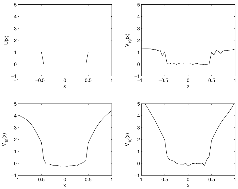
where $p=1,\ldots,n$ and $W_{n}$ are independent zero mean Gaussian random variables with covariance matrix $\sigma^{2}I$ and $F_{n}\in\mathbb{R}^{2}$ are the standard control inputs. Note in general $M$ cannot satisfy (H), but truncation (and suitable re-normalization) of $M$ to any bounded interval of $\mathsf{X}$ does allow (H) to be satisfied. Let also the state-dependent part of the stage cost be $U(x)=(1-\boldsymbol{\mathbb{I}}_{\left(-\delta,\delta\right)}(x\left(1\right)))$ for some $\delta>0$ . This type of cost penalizes states outside $(-\delta,\delta)$ and can be a convenient choice for various containment problems. For this example we will set $X_{0}$ to be zero mean Gaussian random variables with covariance matrix $\left[\begin{array}[]{cc}3&0\\ 0&1\end{array}\right]$ . In Figure 3 we present estimated some value functions for $T=2n=20$ , $\tau=0.1$ , $\delta=0.5$ and $N=500$ . Note that the displayed value function estimates are obtained by averaging over $50$ independent multiple runs as due to the high variance of the initial condition the estimates $h_{p,2n}^{N}$ exhibit a significant amount of variance. Still some errors are visible in the form or ripples due to using a small $N$ .

Infinite Horizon

We will now look at a different infinite horizon scalar example. The Cox-Ingersoll-Ross process satisfies

dX_{t}=\theta\left(\mu-X_{t}\right)dt+\sigma\sqrt{X_{t}}dW_{t},

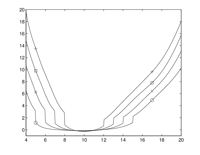
where $\left\{W_{t}\right\}$ is standard one-dimensional Brownian motion, $\theta>0$ is the reversion rate, $\mu>0$ is the level of mean reversion and $\sigma>0$ specifies the volatility. In financial applications this process is widely used to model interest rates. When $2\theta\mu>\sigma^{2}$ it is stationary. Here $\mathsf{X}=\mathbb{R}^{+}$ and for purposes of illustration we consider the case that $M$ is the transition probability from time $t=0$ to $t=0.01$ of the CIR process, which is available in closed form (Cox et al., 1985). Although known to satisfy a type of multiplicative Lyapunov drift condition which allows an MET to be established in a weighted $\infty$ -norm setting (Whiteley et al., 2012), $M$ cannot satisfy (H). Truncation (and suitable re-normalization) of $M$ to any bounded interval of $\mathsf{X}$ does allow (H) to be satisfied. In our numerical experiments this truncation was made to $[0,500]$ . We took the parameter settings $\theta=2$ , $\sigma=20,$ $\mu=10$ and considered, for a range of $\delta$ , the following “well-shaped” cost function:

U(x)=2\mathbb{I}_{[0,10-\delta]}(x)+\mathbb{I}_{\left[10+\delta,\infty\right)}(x),

(51)

which penalizes states outside $(10-\delta,10+\delta)$ .

Figure 4 shows estimates of the value function, which were obtained via averaging by evaluating the window-averaged quantities $\frac{1}{m}\sum_{p=0}^{m-1}h_{n+p,2n}^{N}(x)$ with $N=500$ , $n=2000$ and $m=100$ and evaluations on a fine grid from $x=4$ to $x=20$ . Note the coincidence of the discontinuities in (51) with those in the estimated function. The influence of the parameter $\delta$ is apparent. Table 1 shows the empirical relative variance (variance over the square of the mean) of the estimated value function evaluations at different points $x$ and for different numbers of particles $N$ . The variance evidently decreases with $N$ , with large values associated with more extreme values of $x$ .

N	$x$
N	6	8	10	12	14	16
50	$1.81\times 10^{-3}$	$1.94\times 10^{-5}$	$5.62\times 10^{-5}$	$7.27\times 10^{-5}$	$1.07\times 10^{-3}$	$7.2\times 10^{-3}$
100	$1.02\times 10^{-3}$	$9.13\times 10^{-6}$	$2.78\times 10^{-5}$	$3.26\times 10^{-5}$	$5.41\times 10^{-4}$	$6.15\times 10^{-3}$
500	$1.15\times 10^{-4}$	$4.95\times 10^{-6}$	$1.46\times 10^{-6}$	$5.75\times 10^{-6}$	$3.08\times 10^{-5}$	$2.28\times 10^{-3}$

Table 1: Empirical relative variance of value function evaluations (at different

x

), with

n=2000

from

500

independent realizations of the algorithm.

6 Discussion

We presented a generic particle algorithm to approximate the principle eigen-function of an un-normalized positive Markov integral kernel together with the associated twisted probability kernel. As per standard Perron-Frobenius theory, we have not made any reversibility assumptions, and this is reflected to some extent in the “forward-backward” structure of the algorithm. We also presented some theoretical results demonstrating the validity of using such a numerical scheme and saw how it can be applied to a variety of practical problems.

There are a number of possible avenues for further investigation. Regarding the theory, Assumption (H) is very restrictive when $\mathsf{X}$ is non-compact. Starting points for the analysis of the method under weaker assumptions are (Whiteley, 2013; Whiteley et al., 2012), where the stability of Feynman-Kac semigroups and particle approximations have been studied under a relaxation of the uniform majorization/minorization structure of (H), using a Lyapunov drift condition.

There also many aspects of the applications considered here that could benefit from further study. The connection to optimal importance sampling schemes for rare event simulation and estimation could be extended by studying in detail the variance of the estimator appearing in Proposition 4 as well as the propagation of chaos properties associated with blocks of samples drawn from $\left(P_{(p,n)}^{N}\right)$ . Furthermore, it is of some interest to investigate how optimization schemes such as those in (Kantas, 2009, Chapter 5) could be combined with the algorithm in order to estimate the solution of $\Lambda_{\star}^{\prime}(\alpha)=\delta$ . Regarding this last point, when the solution of $\alpha$ is not unique (Chan and Lai, 2011) by-pass the computation of the eigen-function using saddle-point approximations, so it would be interesting to investigate how the two approaches could be combined. Furthermore, the optimal control problem underlying the Bellman equation in Section 3.2 has only recently received some mathematical attention (Theodorou et al., 2010; Dvijotham and Todorov, 2011) for the finite horizon case and could be investigated further. Especially for the infinite horizon case, there are many connections with continuous time control problems (Dai Pra et al., 1996; Sheu, 1984) and further insight could extend the applicability of the numerical tools in this paper.

Appendix A Appendix

A.1 Proofs and auxiliary results for Section 2.2

We now present dome definitions and preliminary results which preface the proof of Theorem 1 . The first is a lemma that establishes uniform bounds on ratio functionals involving iterates of $Q$ . Set $\mathcal{L}^{+}:=\left\{\varphi\in\mathcal{L}:\nu(\varphi)>0\right\}$ .

Lemma 5.

For any $\mu^{\prime}\in\mathcal{P}$ and $\varphi\in\mathcal{L}^{+}$ ,

\inf_{n\geq 1}\inf_{x\in\mathsf{X}}\frac{Q^{\left(n\right)}(\varphi)(x)}{\mu^{\prime}Q^{\left(n\right)}(\varphi)}\geq\frac{\epsilon^{-}}{\epsilon^{+}}>0,\quad\sup_{n\geq 1}\sup_{x\in\mathsf{X}}\frac{Q^{\left(n\right)}(\varphi)(x)}{\mu^{\prime}Q^{\left(n\right)}(\varphi)}\leq\frac{\epsilon^{+}}{\epsilon^{-}}<\infty.

(52)

Proof.

Under (H),

\frac{Q^{\left(n\right)}\left(\varphi\right)(y)}{Q^{\left(n\right)}\left(\varphi\right)(x)}\leq\frac{\epsilon^{+}}{\epsilon^{-}}\quad\forall x,y\in\mathsf{X},n\geq 1,

then integrating in the numerator with respect to $\mu^{\prime}$ and re-arranging gives the infimum bound in (52). The proof of the supremum bound is similar. ∎

Following Nummelin (2004), the notions of irreducibility and aperiodicity of a non-negative kernel generalize naturally from the probabilistic case, and are expressed in terms of a $\sigma$ -finite irreducibility measure. For simplicity of presentation we shall take as this measure the $\nu$ appearing in (H). It follows immediately from the definitions of (Nummelin, 2004) that when (H) holds, $Q$ is $\nu$ -irreducible and aperiodic. The number $\lambda_{\star}$ as defined in (6)-(7) is called the generalized principal eigen-value (g.p.e.) of $Q$ by Kontoyiannis and Meyn (2003, Theorem 3.1) and in our setting coincides with the reciprocal of the convergence parameter of Nummelin (2004, Section 3.2).

Recall, the spectral radius of $Q$ as a bounded linear operator on $\mathcal{L}$ is defined as $\xi:=\lim_{n\rightarrow\infty}\interleave Q^{\left(n\right)}\interleave^{1/n}$ (existence follows by sub-multiplicativity of operator norm). For notational convenience define $s^{-}:\mathsf{X}\rightarrow\mathbb{R}_{+}$ , $s^{+}:\mathsf{X}\rightarrow\mathbb{R}_{+}$ by $s^{-}(x)=\epsilon^{-},s^{+}(x)=\epsilon^{+},\forall x$ , respectively. In the terminology Nummelin (2004, Proposition 3.4), $Q$ is called $\lambda_{\star}$ -recurrent if and only if $\sum_{n=0}^{\infty}\lambda_{\star}^{-n}\nu Q^{\left(n\right)}\left(s^{-}\right)=\infty$ . The following lemma prepares for Theorem 1.

Lemma 6.

We have

\epsilon^{-}\leq\xi=\lambda_{\star}\leq\epsilon^{+},\quad\quad\qquad\inf_{\mu^{\prime}\in\mathcal{P}}\inf_{n\geq 0}\frac{\mu^{\prime}Q^{\left(n\right)}(1)}{\lambda_{\star}^{n}}>0,

(53)

and therefore $Q$ is $\lambda_{\star}$ -recurrent.

Remark 11.

Following the terminology and arguments of (Nummelin, 2004, p.96), under (H) the kernel $Q$ is then additionally uniformly $\lambda_{\star}$ -recurrent.

Proof.

The upper and lower bounds on the spectral radius $\xi$ follow from (H), because for any $n\geq 1$ and $x\in\mathsf{X}$ we have $\epsilon^{-}\leq\left[Q^{(n)}(1)(x)\right]^{1/n}\leq\epsilon^{+}$ . To verify that $\lambda_{\star}$ coincides with $\xi$ , write

	$\displaystyle\left\|\frac{1}{n}\log\frac{\sup_{x}Q^{(n)}(1)(x)}{\nu Q^{(n)}(s^{-})}\right\|$	$\displaystyle=$	$\displaystyle\left\|\frac{1}{n}\log\frac{\sup_{x}Q^{(n)}(1)(x)}{\nu Q^{(n)}(1)}-\frac{1}{n}\log\epsilon^{-}\right\|$
		$\displaystyle\leq$	$\displaystyle\frac{1}{n}\log\frac{\epsilon^{+}}{\epsilon^{-}}+\frac{1}{n}\log\frac{\nu Q^{(n-1)}(1)}{\nu Q^{(n-1)}(1)}+\frac{1}{n}\left\|\log\epsilon^{-}\right\|\;\rightarrow\;0\text{\quad\ as\quad\ $n\rightarrow\infty$. }$

It remains to verify the uniform lower bound in (53) and thus the $\lambda_{\star}$ -recurrence. A key feature of the majorization part of assumption (H) is that it implies $\nu Q^{\left(n+m-1\right)}\left(s^{+}\right)\leq\nu Q^{\left(n-1\right)}\left(s^{+}\right)\nu Q^{\left(m-1\right)}\left(s^{+}\right)$ and then by sub-additivity we are assured of the existence of:

\Lambda_{\star}^{+}:=\lim_{n\rightarrow\infty}\frac{1}{n}\log\nu Q^{\left(n-1\right)}\left(s^{+}\right)=\inf_{n\geq 1}\frac{1}{n}\log\nu Q^{\left(n-1\right)}\left(s^{+}\right).

(54)

But from the definitions of $s^{+}$ and $s^{-},$

	$\displaystyle\frac{1}{n}\log\nu Q^{\left(n-1\right)}\left(s^{+}\right)-\frac{1}{n}\log\nu Q^{\left(n-1\right)}\left(s^{-}\right)$	$\displaystyle=$	$\displaystyle\frac{1}{n}\log\left[\frac{\nu Q^{\left(n-1\right)}(1)}{\nu Q^{\left(n-1\right)}(1)}\frac{\epsilon^{+}}{\epsilon^{-}}\right]$		(55)
		$\displaystyle=$	$\displaystyle\frac{1}{n}\log\left(\frac{\epsilon^{+}}{\epsilon^{-}}\right),$		(55)

so taking $n\rightarrow\infty$ we find that $\Lambda_{\star}^{+}=\Lambda_{\star}$ , and then (55) together with the right-most equality in (54) imply

\frac{1}{n}\log\nu Q^{\left(n-1\right)}\left(s^{-}\right)-\Lambda_{\star}\geq-\frac{1}{n}\log\left(\frac{\epsilon^{+}}{\epsilon^{-}}\right),

\frac{\nu Q^{\left(n-1\right)}\left(s^{-}\right)}{\lambda_{\star}^{n}}\geq\frac{\epsilon^{-}}{\epsilon^{+}}>0.

Equation (53) then holds as $\frac{\mu^{\prime}Q^{\left(n\right)}(1)}{\nu Q^{\left(n\right)}(1)\epsilon^{+}}\geq\frac{\epsilon^{-}}{\left(\epsilon^{+}\right)^{2}}$ for all $\mu^{\prime}\in\mathcal{P}$ , and this implies $\lambda_{\star}$ -recurrence. ∎

Now consider the family of potential kernels, $\left\{U_{\theta};\theta\in[\lambda_{\star},\infty)\right\}$ ,

U_{\theta}:=\sum_{n=0}^{\infty}\theta^{-n-1}\left(Q-s^{-}\otimes\nu\right)^{\left(n\right)}.

where the convergence of the sum, in the operator norm, is ensured by the $\lambda_{\star}$ -recurrence of $Q$ (shown in Lemma 6 in Appendix) and is straightforward to verify using the inversion argument of Kontoyiannis and Meyn (2003, Proof of Lemma 3.2), noting that as per Lemma 6, the spectral radius of $Q$ coincides with the g.p.e., $\xi=\lambda_{\star}$ .

Proof.

(of Theorem 1) As per Lemma 6, the spectral radius of $Q$ coincides with $\lambda_{\star}$ . By the same Lemma, $Q$ is $\lambda_{\star}-$ recurrent. By (Nummelin, 2004, Theorems 5.1 and 5.2), $\nu U_{\lambda_{\star}}$ and $U_{\lambda_{\star}}(s^{-})$ are then respectively the unique measure and $\nu$ -essentially unique non-zero function satisfying

\nu U_{\lambda_{\star}}Q=\lambda_{\star}\nu U_{\lambda_{\star}},\quad QU_{\lambda_{\star}}(s^{-})=\lambda_{\star}U_{\lambda_{\star}}(s^{-}),\quad\nu U_{\lambda_{\star}}\left(s^{-}\right)=1.

(56)

Under (H) we then have from (56) that

0<\frac{\epsilon^{-}}{\lambda_{\star}}=\frac{\epsilon^{-}}{\lambda_{\star}}\nu U_{\lambda_{\star}}(s^{-})\leq U_{\lambda_{\star}}(s^{-})(x)\leq\frac{\epsilon^{+}}{\lambda_{\star}}\nu U_{\lambda_{\star}}(s^{-})=\frac{\epsilon^{+}}{\lambda_{\star}}<\infty,\quad\forall x,

(57)

thus we take

\eta_{\star}:=\frac{\nu U_{\lambda_{\star}}}{\nu U_{\lambda_{\star}}\left(1\right)},\quad\quad h_{\star}:=\frac{U_{\lambda_{\star}}\left(s^{-}\right)}{\eta_{\star}U_{\lambda_{\star}}\left(s^{-}\right)}

(58)

establishing (8). The uniqueness properties transfer directly to $\eta_{\star}$ and $h_{\star}$ .

We obtain from (56) and (57) the following uniform lower and upper bounds on $h_{\star}$ :

h_{\star}(x)=\frac{Q\left(h_{\star}\right)(x)}{\lambda_{\star}}\geq\frac{\epsilon^{-}}{\lambda_{\star}}\nu\left(h_{\star}\right)=\frac{\epsilon^{-}}{\lambda_{\star}}\frac{\nu U_{\lambda_{\star}}\left(s^{-}\right)}{\eta_{\star}U_{\lambda_{\star}}\left(s^{-}\right)}=\frac{\epsilon^{-}}{\lambda_{\star}}\frac{1}{\eta_{\star}U_{\lambda_{\star}}\left(s^{-}\right)}\geq\frac{\epsilon^{-}}{\epsilon^{+}}>0,\quad\forall x,

(59)

h_{\star}(x)=\frac{Q\left(h_{\star}\right)(x)}{\lambda_{\star}}\leq\frac{\epsilon^{+}}{\lambda_{\star}}\nu\left(h_{\star}\right)=\frac{\epsilon^{+}}{\lambda_{\star}}\frac{1}{\eta_{\star}U_{\lambda_{\star}}\left(s^{-}\right)}\leq\frac{\epsilon^{+}}{\epsilon^{-}}<\infty,\quad\forall x

(60)

so that (9) is established. Furthermore $P_{\star}$ is then well-defined as a Markov kernel and we readily verify that it satisfies a uniform minorization condition:

$\displaystyle P_{\star}(x,dx^{\prime})$	$\displaystyle=$	$\displaystyle\frac{Q(x,dx^{\prime})h_{\star}(x^{\prime})}{h_{\star}(x)\lambda_{\star}}$
	$\displaystyle\geq$	$\displaystyle\frac{\nu(h_{\star})}{h_{\star}(x)\lambda_{\star}}\frac{\epsilon^{-}\nu(dx^{\prime})h_{\star}(x^{\prime})}{\nu(h_{\star})}$
	$\displaystyle=$	$\displaystyle\frac{1}{U_{\lambda_{\star}}\left(s^{-}\right)(x)\lambda_{\star}}\epsilon^{-}\nu(dx^{\prime})U_{\lambda_{\star}}\left(s^{-}\right)(x^{\prime})$
	$\displaystyle\geq$	$\displaystyle\frac{\epsilon^{-}}{\epsilon^{+}}\nu(dx^{\prime})U_{\lambda_{\star}}\left(s^{-}\right)(x^{\prime}),\quad\forall x,$

where $\nu U_{\lambda_{\star}}\left(s^{-}\right)=1$ and (57) have been used. Thus $P_{\star}$ is uniformly geometrically ergodic and by inspection of the eigen-measure equation its unique invariant probability distribution, denoted by $\pi_{\star}$ , is given by $\pi_{\star}\left(\varphi\right)=\eta_{\star}\left(h_{\star}\varphi\right)/\eta_{\star}\left(h_{\star}\right)=\eta_{\star}\left(h_{\star}\varphi\right)$ . Then, again noting that $\nu U_{\lambda_{\star}}\left(s^{-}\right)=1$ , by (Meyn and Tweedie, 2009, Theorem 16.2.4) we have:

\interleave P_{\star}^{\left(n\right)}-1\otimes\pi_{\star}\interleave\leq 2\rho^{n},

(61)

where $\rho:=1-\left(\epsilon^{-}/\epsilon^{+}\right)$ , which establishes (10). Multiplying by $h_{\star}>0$ in (61) yields for any $\phi\in\mathcal{L},x\in\mathsf{X}$ ,

\left|\lambda_{\star}^{-n}Q^{\left(n\right)}\left(h_{\star}\phi\right)(x)-h_{\star}(x)\eta_{\star}\left(h_{\star}\phi\right)\right|\leq 2\rho^{n}h_{\star}(x)\left\|\phi\right\|\leq 2\rho^{n}\left(\frac{\epsilon^{+}}{\epsilon^{-}}\right)\left\|\phi\right\|,

(62)

where (60) has been used. By equation (59), $h_{\star}$ is bounded below away from zero and therefore for any $\varphi\in\mathcal{L}$ , we may have taken $\phi:=\varphi/h_{\star}\in\mathcal{L}$ in (62). Finally noting from (59) that $\left\|\varphi/h_{\star}\right\|\leq\left(\epsilon^{+}/\epsilon^{-}\right)\left\|\varphi\right\|$ , the bound of (11) is established. ∎

A.2 Proofs and auxiliary results for Section 2.3

Under assumption (H) we obtain uniform bounds on these quantities, as per the following Lemma.

Lemma 7.

\inf_{n\geq 0}\eta_{n}(G)>0

(63)

\inf_{n\geq 1}\inf_{0\leq p\leq n}\inf_{x\in\mathsf{X}}h_{p,n}(x)\geq\frac{\epsilon^{-}}{\epsilon^{+}}>0,\quad\sup_{n\geq 1}\sup_{0\leq p\leq n}\sup_{x\in\mathsf{X}}h_{p,n}(x)\leq\frac{\epsilon^{+}}{\epsilon^{-}}<\infty.

(64)

Proof.

Assumption (H) implies that $G$ is bounded below away from zero and therefore we have (63). Lemma 5 in the Appendix implies (64). ∎

We proceed with the proof of Proposition 1:

Proof.

(of Proposition 1) We first treat (18),

$\displaystyle\left\\|\eta_{n}-\eta_{\star}\right\\|$	$\displaystyle=$	$\displaystyle\sup_{\varphi:\left\|\varphi\right\|\leq 1}\left\|\mu Q^{\left(n\right)}\left(\varphi\right)\left[\frac{1}{\mu Q^{\left(n\right)}\left(1\right)}-\frac{1}{\lambda_{\star}^{n}\mu(h_{\star})}\right]+\frac{\mu Q^{\left(n\right)}\left(\varphi\right)}{\lambda_{\star}^{n}\mu(h_{\star})}-\eta_{\star}\left(\varphi\right)\right\|$
	$\displaystyle\leq$	$\displaystyle\sup_{\varphi:\left\|\varphi\right\|\leq 1}\left\|\frac{\mu Q^{\left(n\right)}\left(\varphi\right)}{\mu Q^{\left(n\right)}\left(1\right)}\right\|\left\|\frac{\mu Q^{\left(n\right)}\left(1\right)}{\lambda_{\star}^{n}\mu(h_{\star})}-1\right\|$
		$\displaystyle+\sup_{\varphi:\left\|\varphi\right\|\leq 1}\left\|\frac{\mu Q^{\left(n\right)}\left(\varphi\right)}{\lambda_{\star}^{n}\mu(h_{\star})}-\eta_{\star}\left(\varphi\right)\right\|$
	$\displaystyle\leq$	$\displaystyle\frac{2}{\mu(h_{\star})}\rho^{n}\left(\frac{\epsilon^{+}}{\epsilon^{-}}\right)^{2}$
		$\displaystyle+\frac{2}{\mu(h_{\star})}\rho^{n}\left(\frac{\epsilon^{+}}{\epsilon^{-}}\right)^{2}$
	$\displaystyle\leq$	$\displaystyle 4\rho^{n}\left(\frac{\epsilon^{+}}{\epsilon^{-}}\right)^{3},$

where the penultimate inequality follows from two applications of the bound of Theorem 1, Equation (11), and the final inequality is due to (9). This establishes (18).

In order to prove (19), we first consider products of the values $\left(\lambda_{n}\right)$ . We have

$\displaystyle\left\|\frac{\prod_{\ell=p}^{n-1}\lambda_{\ell}}{\lambda_{\star}^{n-p}}-1\right\|$	$\displaystyle=$	$\displaystyle\left\|\frac{\eta_{p}Q^{\left(n-p\right)}(1)}{\lambda_{\star}^{n-p}}-\eta_{p}(h_{\star})+\eta_{p}(h_{\star})-\eta_{\star}(h_{\star})\right\|$	(65)
	$\displaystyle\leq$	$\displaystyle\left\|\frac{\eta_{p}Q^{\left(n-p\right)}(1)}{\lambda_{\star}^{n-p}}-\eta_{p}(h_{\star})\right\|+\left\|\eta_{p}(h_{\star})-\eta_{\star}(h_{\star})\right\|$
	$\displaystyle\leq$	$\displaystyle 2\rho^{n-p}\left(\frac{\epsilon^{+}}{\epsilon^{-}}\right)^{2}+4\rho^{p}\left(\frac{\epsilon^{+}}{\epsilon^{-}}\right)^{3}\left\\|h_{\star}\right\\|$
	$\displaystyle\leq$	$\displaystyle 2\rho^{\left(n-p\right)\wedge p}\left(\frac{\epsilon^{+}}{\epsilon^{-}}\right)^{2}\left(1+2\left(\frac{\epsilon^{+}}{\epsilon^{-}}\right)^{2}\right)$

where the penultimate inequality is due to (11) of Theorem 1 and (18), and the final inequality is due to (9). Integrating and iterating the eigen-measure equation (58) gives $\lambda_{\star}^{n}=\eta_{\star}Q^{n}(1)$ . Then by Lemma 5,

\sup_{n\geq 1}\sup_{x\in\mathsf{X}}\frac{Q^{\left(n\right)}(1)(x)}{\lambda_{\star}^{n}}\leq\frac{\epsilon^{+}}{\epsilon^{-}}.

(66)

With the above bounds in hand we now address (19). We have

$\displaystyle\left\|h_{p,n}(x)-h_{\star}(x)\right\|$	$\displaystyle=$	$\displaystyle\left\|\frac{Q^{\left(n-p\right)}(1)(x)}{\lambda_{\star}^{n-p}}\left(\frac{\lambda_{\star}^{n-p}}{\prod_{\ell=p}^{n-1}\lambda_{\ell}}-1\right)+\frac{Q^{\left(n-p\right)}(1)(x)}{\lambda_{\star}^{n-p}}-h_{\star}(x)\right\|$
	$\displaystyle\leq$	$\displaystyle\left\|\frac{\lambda_{\star}^{n-p}}{\prod_{\ell=p}^{n-1}\lambda_{\ell}}-1\right\|\sup_{m\geq 1}\sup_{y\in\mathsf{X}}\frac{Q^{\left(m\right)}(1)(y)}{\lambda_{\star}^{m}}$
		$\displaystyle+\left\|\frac{Q^{\left(n-p\right)}(1)(x)}{\lambda_{\star}^{n-p}}-h_{\star}(x)\right\|$
	$\displaystyle\leq$	$\displaystyle 2\rho^{\left(n-p\right)\wedge p}\left(\frac{\epsilon^{+}}{\epsilon^{-}}\right)^{3}\left(1+2\left(\frac{\epsilon^{+}}{\epsilon^{-}}\right)^{2}\right)+2\rho^{n-p}\left(\frac{\epsilon^{+}}{\epsilon^{-}}\right)^{2}$
	$\displaystyle=$	$\displaystyle 2\rho^{\left(n-p\right)\wedge p}\left(\frac{\epsilon^{+}}{\epsilon^{-}}\right)^{2}\left[1+\left(\frac{\epsilon^{+}}{\epsilon^{-}}\right)+2\left(\frac{\epsilon^{+}}{\epsilon^{-}}\right)^{3}\right].$

where for the final inequality, (65), (66) and (11) have been used. This establishes (19).

For (20), consider the decomposition

$\displaystyle\interleave P_{(p,n)}-P_{\star}\interleave$	$\displaystyle\leq$	$\displaystyle\sup_{x}\sup_{\varphi:\left\|\varphi\right\|\leq 1}\left[\frac{1}{\lambda_{p-1}h_{p-1,n}(x)}\left\|Q\left[\left(h_{p,n}-h_{\star}\right)\varphi\right](x)\right\|\right.$
		$\displaystyle+\frac{1}{\lambda_{p-1}}\frac{\left\|h_{p-1,n}(x)-h_{\star}(x)\right\|}{h_{p-1,n}(x)}\frac{\left\|Q\left(h_{\star}\varphi\right)(x)\right\|}{h_{\star}(x)}$
		$\displaystyle+\left.\frac{\left\|\lambda_{\star}-\lambda_{p-1}\right\|}{\lambda_{p-1}\lambda_{\star}}\frac{1}{h_{\star}(x)}\left\|Q\left(h_{\star}\varphi\right)(x)\right\|\right]$
	$\displaystyle\leq$	$\displaystyle\left\\|h_{p,n}-h_{\star}\right\\|\sup_{x}\frac{Q(1)(x)}{\lambda_{p-1}h_{p-1,n}(x)}$
		$\displaystyle+\frac{\lambda_{\star}}{\lambda_{p-1}}\left\\|h_{p-1,n}-h_{\star}\right\\|\sup_{x}\frac{1}{h_{p-1,n}(x)}$
		$\displaystyle+\frac{\left\|\lambda_{\star}-\lambda_{p-1}\right\|}{\lambda_{p-1}}$
	$\displaystyle\leq$	$\displaystyle C_{h}\rho^{\left(n-p\right)\wedge p}2\left(\frac{\epsilon^{+}}{\epsilon^{-}}\right)^{2}+C_{\eta}\rho^{p-1}\frac{\epsilon^{+}}{\epsilon^{-}},$

where for the final equality, Lemma 7, the identities $\lambda_{p}=\eta_{p}(G)$ , $\lambda_{\star}=\eta_{\star}(G)$ , and (18)-(19) have been used. ∎

A.3 Proofs and auxiliary results for Section 4.2

A.3.1 Lack of bias

Proof.

(of Proposition 3). The $n=0$ case is trivial. For any $\varphi\in\mathcal{L},$ $n\geq 1$ and $x\in\mathsf{X},$ we have

$\displaystyle\mathbb{E}_{N}\left[\left.Q_{n}^{N}\left(\varphi\right)(x)\right\|\mathcal{F}_{n-1}\right]$	$\displaystyle=$	$\displaystyle\mathbb{E}_{N}\left[\left.\int\frac{\mathrm{d}Q\left(x,\cdot\right)}{\mathrm{d}\Phi\left(\eta_{n-1}^{N}\right)}\left(x^{\prime}\right)\varphi\left(x^{\prime}\right)\eta_{n}^{N}\left(dx^{\prime}\right)\right\|\mathcal{F}_{n-1}\right]$	(67)
	$\displaystyle=$	$\displaystyle\frac{1}{N}\sum_{i=1}^{N}\mathbb{E}_{N}\left[\left.\frac{\mathrm{d}Q\left(x,\cdot\right)}{\mathrm{d}\Phi\left(\eta_{n-1}^{N}\right)}\left(\zeta_{n}^{i}\right)\varphi\left(\zeta_{n}^{i}\right)\right\|\mathcal{F}_{n-1}\right]$
	$\displaystyle=$	$\displaystyle\int\frac{\mathrm{d}Q\left(x,\cdot\right)}{\mathrm{d}\Phi\left(\eta_{n-1}^{N}\right)}\left(x^{\prime}\right)\varphi\left(x^{\prime}\right)\Phi\left(\eta_{n-1}^{N}\right)\left(dx^{\prime}\right)$
	$\displaystyle=$	$\displaystyle Q\left(\varphi\right)(x),$

where the penultimate equality is due to the definition of the particle transition probabilities (34).

Now consider the telescoping decomposition

	$\displaystyle\mu^{N}Q_{0,n}^{N}\left(\varphi\right)-\mu^{\prime}Q^{\left(n\right)}\left(\varphi\right)$	$\displaystyle=$	$\displaystyle\sum_{p=0}^{n-1}\left[\mu^{N}Q_{0,p+1}^{N}Q^{\left(n-p-1\right)}\left(\varphi\right)-\mu^{N}Q_{0,p}^{N}Q^{\left(n-p\right)}\left(\varphi\right)\right]$
			$\displaystyle+\left(\mu^{N}-\mu^{\prime}\right)Q^{\left(n\right)}\left(\varphi\right).$

For each term in the big summation we have

	$\displaystyle\mathbb{E}_{N}\left[\left.\mu^{N}Q_{0,p+1}^{N}Q^{\left(n-p-1\right)}\left(\varphi\right)-\mu^{N}Q_{0,p}^{N}Q^{\left(n-p\right)}\left(\varphi\right)\right\|\mathcal{F}_{p}\right]$
	$\displaystyle=\int\mu^{N}Q_{0,p}^{N}\left(dx_{p}\right)\mathbb{E}\left[\left.Q_{p+1}^{N}Q^{\left(n-p-1\right)}\left(\varphi\right)(x_{p})-Q^{\left(n-p\right)}\left(\varphi\right)(x_{p})\right\|\mathcal{F}_{p}\right]$
	$\displaystyle=0,$

where the final equality is due to (67). For the remaining term, $\mathbb{E}_{N}\left[\left(\mu^{N}-\mu^{\prime}\right)Q^{\left(n\right)}\left(\varphi\right)\right]=0$ by assumption of the proposition. ∎

A.3.2 Path-wise stability

The following proposition provides a generic result on iterates of non-negative kernels, which will serve multiple purposes throughout the remaining proofs in the paper.

Proposition 6.

Let $\left(K_{n};n\geq 1\right)$ be a collection of possibly random, non-negative integral kernels, and suppose that for a collection of possibly random, finite measures $\left(\nu_{n};n\geq 1\right)$ and positive, bounded functions $\left(S_{n}^{-},S_{n}^{+};n\geq 1\right)$ ,

S_{n}^{-}(x)\nu_{n}\left(\cdot\right)\leq K_{n}(x,\cdot)\leq S_{n}^{+}(x)\nu_{n}\left(\cdot\right),\quad\forall x\in\mathsf{X},n\geq 1.

(68)

Then

\sup_{n\geq 1}\sup_{x,x^{\prime}\in\mathsf{X}}\frac{K_{0,n}(1)(x)}{K_{0,n}(1)(x^{\prime})}\leq\sup_{n\geq 1}\overline{S}_{n},

(69)

where

\overline{S}_{n}:=\sup_{x,x^{\prime}\in\mathsf{X}}\frac{S_{n}^{+}(x)}{S_{n}^{-}(x^{\prime})}.

Furthermore, for any possibly random probability measure $\eta$ and $\varphi\in\mathcal{L},$

\sup_{x\in\mathsf{X}}\left|\frac{K_{0,n}(\varphi)(x)}{\eta K_{0,n}(1)}-\frac{K_{0,n}(1)(x)}{\eta K_{0,n}(1)}\frac{\eta K_{0,n}(\varphi)}{\eta K_{0,n}(1)}\right|\leq\left\|\varphi\right\|2C_{S}\prod_{p=1}^{n}\rho_{p}

where $\rho_{n}:=1-\left(\inf_{x\in\mathsf{X}}\frac{S{}_{n}^{-}(x)}{S_{n}^{+}(x)}\right)^{2}$ and $C_{S}:=\sup_{n\geq 1}\overline{S}_{n}.$

Remark 12.

We approach the proof of this proposition using a decomposition idea of Kleptsyna and Veretennikov (2008), a technique which they demonstrated to be useful in the analysis of non-linear filter stability on non-compact state-spaces. We won’t exploit the full generality of this kind of decomposition (it is useful under conditions much weaker than (H) - see for example (Douc et al., 2009), again in the filtering context) and we choose to take this approach because it yields a short and direct proof, which is sufficient for our purposes.

Proof.

(of Proposition 6). The uniform bound of (69) holds directly under the assumptions of the proposition.

We write $K_{n}^{\otimes 2}\left(x,y,d\left(x^{\prime},y^{\prime}\right)\right):=K_{n}\left(x,dx^{\prime}\right)K_{n}\left(y,dy^{\prime}\right)$ and $\nu_{n}^{\otimes 2}\left(d\left(x,y\right)\right):=\nu_{n}(dx)\nu_{n}(dy)$ . Under the assumptions of the proposition we have for any $\left(x,y\right)\in\mathsf{X}^{2}$ and measurable $A\subset\mathsf{X}^{2}$ such that $\nu_{n}^{\otimes 2}(A)>0$ ,

$\displaystyle\widehat{K}_{n}\left(x,y,A\right)$	$\displaystyle:=$	$\displaystyle K_{n}^{\otimes 2}\left(x,y,A\right)-S{}_{n}^{-}(x)S{}_{n}^{-}(y)\nu_{n}^{\otimes 2}\left(A\right)$	(70)
	$\displaystyle\leq$	$\displaystyle\left[1-\frac{S{}_{n}^{-}(x)S{}_{n}^{-}(y)}{S_{n}^{+}(x)S_{n}^{+}(y)}\right]K_{n}^{\otimes 2}\left(x,y,A\right).$
	$\displaystyle\leq$	$\displaystyle\rho_{n}K_{n}^{\otimes 2}\left(x,y,A\right).$

Furthermore,

	$\displaystyle\left\|\frac{K_{0,n}(\varphi)(x)}{\eta K_{0,n}(1)}-\frac{K_{0,n}(1)(x)}{\eta K_{0,n}(1)}\frac{\eta K_{0,n}(\varphi)}{\eta K_{0,n}(1)}\right\|$
	$\displaystyle=\frac{\left\|K_{0,n}(\varphi)(x)\eta K_{0,n}(1)-K_{0,n}(1)(x)\eta K_{0,n}(\varphi)\right\|}{\eta K_{0,n}(1)\eta K_{0,n}(1)}$
	$\displaystyle=\frac{K_{0,n}(1)(x)}{\eta K_{0,n}(1)}\frac{\left\|\left(\delta_{x}\otimes\eta\right)K_{0,n}^{\otimes 2}\left(\varphi\otimes 1-1\otimes\varphi\right)\right\|}{\left(\delta_{x}\otimes\eta\right)K_{0,n}^{\otimes 2}(1\otimes 1)}$
	$\displaystyle=\frac{K_{0,n}(1)(x)}{\eta K_{0,n}(1)}\frac{\left\|\left(\delta_{x}\otimes\eta\right)\widehat{K}_{0,n}\left(\varphi\otimes 1-1\otimes\varphi\right)\right\|}{\left(\delta_{x}\otimes\eta\right)K_{0,n}^{\otimes 2}(1\otimes 1)}$		(71)
	$\displaystyle\leq 2\left\\|\varphi\right\\|\left(\sup_{p\geq 1}\overline{S}_{p}\right)\frac{\left(\delta_{x}\otimes\eta\right)\widehat{K}_{0,n}\left(1\otimes 1\right)}{\left(\delta_{x}\otimes\eta\right)K_{0,n}^{\otimes 2}(1\otimes 1)}$
	$\displaystyle\leq 2\left\\|\varphi\right\\|\left(\sup_{p\geq 1}\overline{S}_{p}\right)\prod_{p=1}^{n}\rho_{p},$

where the equality in (71) is due to the decomposition technique of Kleptsyna and Veretennikov (2008, p. 422) (see also Douc et al., 2009, Proof of Proposition 12), and for the final two inequalities (69) and (70) have been used. ∎

Under assumption (H), we find that the random operators satisfy path-wise, a regularity condition of a similar form, which is used below in the Proof of Proposition 8.

Lemma 8.

The operators $\left(Q_{n}^{N}\right)$ satisfy

\alpha_{n}^{N}(\cdot)\epsilon^{-}\leq Q_{n}^{N}(x,\cdot)\leq\epsilon^{+}\alpha_{n}^{N}(\cdot),\quad\forall x\in\mathsf{X},n\geq 1,N\geq 1,

(72)

where $\alpha_{n}^{N}$ is the random finite measure:

\alpha_{n}^{N}\left(dx\right):=\eta_{n}^{N}(dx)\left[\frac{\mathrm{d}\Phi\left(\eta_{n-1}^{N}\right)}{\mathrm{d}\nu}(x)\right]^{-1},

and $\epsilon^{-},\epsilon^{+}$ are the deterministic constants in assumption (H). Moreover for all $x\in\mathsf{X}$ and $p\leq n$ ,

\frac{\epsilon^{-}}{\epsilon^{+}}\leq h_{p,n}^{N}(x)\leq\frac{\epsilon^{+}}{\epsilon^{-}},

Proof.

Since $Q(x,\cdot)$ is equivalent to $\nu$ , then $\Phi\left(\eta_{n-1}^{N}\right)$ is too, and it is straightforward to check that assumption (H) implies that $\frac{\mathrm{d}\nu}{\mathrm{d}\Phi\left(\eta_{n-1}^{N}\right)}(x)$ is bounded above and below away from zero in $x$ . We then have

$\displaystyle Q_{n}^{N}(x,A)$	$\displaystyle=$	$\displaystyle\int_{A}\frac{\mathrm{d}Q(x\cdot)}{\mathrm{d}\Phi\left(\eta_{n-1}^{N}\right)}(x^{\prime})\eta_{n}^{N}(dx^{\prime})$
	$\displaystyle=$	$\displaystyle\int_{A}q(x,x^{\prime})\frac{\mathrm{d}\nu}{\mathrm{d}\Phi\left(\eta_{n-1}^{N}\right)}(x^{\prime})\eta_{n}^{N}(dx^{\prime})$
	$\displaystyle\leq$	$\displaystyle\epsilon^{+}\int_{A}\frac{\mathrm{d}\nu}{\mathrm{d}\Phi\left(\eta_{n-1}^{N}\right)}(x^{\prime})\eta_{n}^{N}(dx^{\prime}),$

The proof of the lower bound is similar. The bounds for $h_{p,n}^{N}(x)=Q_{p,n}^{N}(1)(x)/\eta_{p}^{N}Q_{p,n}^{N}(1)$ follow from (72). ∎

Proof.

(of Theorem 3) From Lemma 4,

\prod_{p=0}^{n-1}\lambda_{p}^{N}=\eta_{0}^{N}Q_{0,n}^{N}\left(1\right),\quad\quad h_{0,n}^{N}=\frac{Q_{0,n}^{N}\left(1\right)}{\eta_{0}^{N}Q_{0,n}^{N}\left(1\right)},\quad\quad\eta_{n}^{N}=\frac{\eta_{0}^{N}Q_{0,n}^{N}}{\eta_{0}^{N}Q_{0,n}^{N}\left(1\right)}.

(73)

Thus (42) holds due to Lemma 8 and Proposition 6 applied with $\eta=\eta_{0}^{N}$ , $K_{n}=Q_{n}^{N},$ $\nu_{n}=\alpha_{n}^{N}$ and $S_{n}^{+}=\epsilon^{+},S_{n}^{-}=\epsilon^{-}$ are constant. Dividing through by $\mu^{\prime}\left(h_{0.n}^{N}\right)$ in (42), again noting (73) and using

\sup_{n\geq 1}\sup_{x,x^{\prime}\in\mathsf{X}}\frac{Q_{0,n}^{N}(1)(x)}{Q_{0,n}^{N}(1)(x^{\prime})}\leq\frac{\epsilon^{+}}{\epsilon^{-}},

(74)

which also holds by Proposition 6, we establish (43). ∎

A.4 Auxiliary results and proof of Theorem 4

Consider the collection of “backward” random kernels $\left(R_{n}^{N}\right)$ defined by

\displaystyle R_{n}^{N}\left(x,dx^{\prime}\right)

\displaystyle:=

\displaystyle\eta_{n-1}^{N}(dx^{\prime})\frac{dQ(x^{\prime},\cdot)}{d\Phi\left(\eta_{n-1}^{N}\right)}(x),\quad n\geq 1,

and with a slight abuse of convention, write

R_{n,n}^{N}:=Id,\quad\quad R_{n,p}^{N}:=R_{n}^{N}R_{n-1}^{N}\cdots R_{p+1}^{N},\quad p<n.

The interest in these quantities is that, in the context of the $L_{r}$ error estimates which are the focus of this section, they provide a convenient way to express the functions $\left(h_{p,n}^{N}\right)$ and share path-wise stability properties with $\left(Q_{n}^{N}\right)$ . Indeed by a simple induction it can be shown that for any $\varphi\in\mathcal{L}$ ,

\eta_{n}^{N}R_{n,p}^{N}\left(\varphi\right)=\eta_{p}^{N}\left[\varphi Q_{p,n}^{N}(1)\right],\quad p\leq n.

(75)

Remark 13.

Each kernel $R_{n}^{N}$ is equal, up to a scaling factor of $\eta_{n-1}^{N}(G)$ , to a certain “backward” Markov kernel used in the analysis of Del Moral et al. (2010). In contrast to the latter work, we are centrally concerned with emphasizing the relationship between $\left(Q_{p,n}^{N}\right)$ and the underlying semigroup $\left(Q^{(n)}\right)$ . In view of (75) and Proposition 3, we therefore prefer to deal with $\left(R_{n}^{N}\right)$ , but only for cosmetic reasons.

The $\left(R_{n}^{N}\right)$ satisfy a condition similar to that in Lemma 8, as per the following Lemma.

Lemma 9.

The operators $\left(R_{n}^{N}\right)$ satisfy

\eta_{n-1}^{N}(\cdot)\beta_{n}^{N}(x)\epsilon^{-}\leq R_{n}^{N}(x,\cdot)\leq\epsilon^{+}\beta_{n}^{N}(x)\eta_{n-1}^{N}(\cdot),\quad\forall x\in\mathsf{X},n\geq 1,N\geq 1,

where $\beta_{n}^{N}$ is the random, positive and bounded function:

\beta_{n}^{N}\left(x\right):=\left[\frac{\mathrm{d}\Phi\left(\eta_{n-1}^{N}\right)}{\mathrm{d}\nu}(x)\right]^{-1},

and $\epsilon^{-},\epsilon^{+}$ are the deterministic constants in assumption (H).

Proof.

From definitions,

$\displaystyle R_{n}^{N}(x,A)$	$\displaystyle=$	$\displaystyle\int_{A}\frac{\mathrm{d}Q(x^{\prime},\cdot)}{\mathrm{d}\Phi\left(\eta_{n-1}^{N}\right)}(x)\eta_{n-1}^{N}(dx^{\prime})$
	$\displaystyle=$	$\displaystyle\int_{A}\frac{\mathrm{d}Q(x^{\prime},\cdot)}{\mathrm{d}\nu}\frac{d\nu}{\Phi\left(\eta_{n-1}^{N}\right)}(x)\eta_{n-1}^{N}(dx^{\prime})$
	$\displaystyle\leq$	$\displaystyle\epsilon^{+}\frac{\mathrm{d}\nu}{\mathrm{d}\Phi\left(\eta_{n-1}^{N}\right)}(x)\eta_{n-1}^{N}\left(A\right).$

The claimed positivity and boundedness of $\beta_{n}^{N}$ follows from (H). The proof of the lower bound is similar. ∎

It is well known that under (H) and variations thereof, one can obtain time-uniform $L_{r}$ estimates for errors of the form $\eta_{n}^{N}(\varphi)-\eta_{n}\left(\varphi\right)$ . We will make use of the following result, due to Del Moral (2004, Theorem 7.4.4). The proof is omitted.

Proposition 7.

For any $r\geq 1$ there exists a universal constant $B_{r}$ such that for any $\varphi\in\mathcal{L},$ the following time uniform estimate holds

\sup_{n\geq 0}\mathbb{E}_{N}\left[\left|\eta_{n}^{N}\left(\varphi\right)-\eta_{n}\left(\varphi\right)\right|^{r}\right]^{1/r}\leq 2\left\|\varphi\right\|\frac{B_{r}}{\sqrt{N}}\left(\frac{\epsilon^{+}}{\epsilon^{-}}\right)^{5}.

We need a further definition. Consider now the functions $\left(\phi_{n}\right)$ and their random counterparts $\left(\phi_{n}^{N}\right)$ defined by

\phi_{n}\left(x,x^{\prime}\right):=\frac{dQ\left(x,\cdot\right)}{d\eta_{n}Q}\left(x^{\prime}\right),\quad\quad\phi_{n}^{N}\left(x,x^{\prime}\right):=\frac{dQ\left(x,\cdot\right)}{d\eta_{n}^{N}Q}\left(x^{\prime}\right),\quad n\geq 0

and note that under (H),

\sup_{n\geq 0}\sup_{x,x^{\prime}}\left|\phi_{n}\left(x,x^{\prime}\right)\right|\leq\frac{\epsilon^{+}}{\epsilon^{-}},\quad\quad\sup_{N\geq 1}\sup_{n\geq 0}\sup_{x,x^{\prime}}\left|\phi_{n}^{N}\left(x,x^{\prime}\right)\right|\leq\frac{\epsilon^{+}}{\epsilon^{-}}.

(76)

Furthermore, we then have from definitions that

	$\displaystyle h_{p,n}^{N}(x)$	$\displaystyle=$	$\displaystyle\frac{Q_{p,n}^{N}(1)(x)}{\eta_{p}^{N}Q_{p,n}^{N}(1)}=\frac{1}{\eta_{p+1}^{N}Q_{p+1,n}^{N}(1)}\int\frac{dQ\left(x,\cdot\right)}{d\eta_{p}^{N}Q}\left(x^{\prime}\right)Q_{p+1,n}^{N}(1)(x^{\prime})\eta_{p+1}^{N}\left(dx^{\prime}\right)$		(77)
			$\displaystyle=\frac{\eta_{n}^{N}R_{n,p+1}^{N}\left[\phi_{p}^{N}\left(x,\cdot\right)\right]}{\eta_{n}^{N}R_{n,p+1}^{N}\left(1\right)},$		(77)

where the final equality is due to (75).

Proposition 8.

For any $r\geq 1$ there exists a universal constant $B_{r}$ such that for any $\varphi\in\mathcal{L}$ and $N\geq 1$ ,

\sup_{p\leq n}\sup_{x\in\mathsf{X}}\mathbb{E}_{N}\left[\left|\frac{Q_{p}^{N}(\varphi h_{p,n}^{N})(x)}{\lambda_{p-1}^{N}}-\frac{Q(\varphi h_{p,n})(x)}{\lambda_{p-1}}\right|^{r}\right]^{1/r}\leq 2\left\|\varphi\right\|\frac{B_{r}}{\sqrt{N}}\tilde{C},

where

\tilde{C}=\left[3\left(\frac{\epsilon^{+}}{\epsilon^{-}}\right)^{7}+\left(\frac{\epsilon^{+}}{\epsilon^{-}}\right)^{5}\frac{1}{1-\tilde{\rho}}\right],

and $\tilde{\rho}$ is as in Theorem 3.

Proof.

(of Proposition 8) From the identities

\frac{Q_{p}^{N}(\varphi h_{p,n}^{N})(x)}{\lambda_{p-1}^{N}}=\frac{\eta_{p}^{N}\left[\varphi\phi_{p-1}^{N}\left(x,\cdot\right)Q_{p,n}^{N}(1)\right]}{\eta_{p}^{N}Q_{p,n}^{N}(1)}=\frac{\eta_{n}^{N}R_{n,p}^{N}\left[\varphi\phi_{p-1}^{N}\left(x,\cdot\right)\right]}{\eta_{n}^{N}R_{n,p}^{N}\left(1\right)}

(established similarly to equation (77)) and

\frac{Q(\varphi h_{p,n})}{\lambda_{p-1}}(x)=\frac{\eta_{p}\left[\varphi\phi_{p-1}\left(x,\cdot\right)Q^{(n-p)}(1)\right]}{\eta_{p}Q^{\left(n-p\right)}(1)},

we have the decomposition

\frac{Q_{p}^{N}(\varphi h_{p,n}^{N})(x)}{\lambda_{p-1}^{N}}-\frac{Q(\varphi h_{p,n})(x)}{\lambda_{p-1}}=\sum_{j=1}^{3}T_{p,n}^{N,j}(x)

where

$\displaystyle T_{p,n}^{N,1}(x)$	$\displaystyle:=$	$\displaystyle\frac{\eta_{n}^{N}R_{n,p}^{N}\left[\varphi\left(\phi_{p-1}^{N}\left(x,\cdot\right)-\phi_{p-1}\left(x,\cdot\right)\right)\right]}{\eta_{n}^{N}R_{n,p}^{N}\left(1\right)}$	(78)
$\displaystyle T_{p,n}^{N,2}(x)$	$\displaystyle:=$	$\displaystyle\frac{\eta_{n}^{N}R_{n,p}^{N}\left[\varphi\phi_{p-1}\left(x,\cdot\right)\right]}{\eta_{n}^{N}R_{n,p}^{N}\left(1\right)}-\frac{\Phi\left(\eta_{p-1}^{N}\right)\left[\varphi\phi_{p-1}\left(x,\cdot\right)Q^{(n-p)}(1)\right]}{\Phi\left(\eta_{p-1}^{N}\right)Q^{\left(n-p\right)}(1)}$	(79)
$\displaystyle T_{p,n}^{N,3}(x)$	$\displaystyle:=$	$\displaystyle\frac{\Phi\left(\eta_{p-1}^{N}\right)\left[\varphi\phi_{p-1}\left(x,\cdot\right)Q^{(n-p)}(1)\right]}{\Phi\left(\eta_{p-1}^{N}\right)Q^{\left(n-p\right)}(1)}-\frac{\eta_{p}\left[\varphi\phi_{p-1}\left(x,\cdot\right)Q^{(n-p)}(1)\right]}{\eta_{p}Q^{\left(n-p\right)}(1)}.$	(80)

For the difference in (78), under (H) we have

$\displaystyle\sup_{x\in\mathsf{X}}\left\|T_{p,n}^{N,1}(x)\right\|$	$\displaystyle\leq$	$\displaystyle\frac{\left\\|\varphi\right\\|\epsilon^{+}}{\eta_{n}^{N}R_{n,p}^{N}\left(1\right)}\int\left\|\frac{1}{\int\eta_{p-1}^{N}(dy)q\left(y,x^{\prime}\right)}-\frac{1}{\int\eta_{p-1}(dy)q\left(y,x^{\prime}\right)}\right\|\eta_{n}^{N}R_{n,p}^{N}\left(dx^{\prime}\right)$
	$\displaystyle\leq$	$\displaystyle\frac{\left\\|\varphi\right\\|\epsilon^{+}}{\eta_{n}^{N}R_{n,p}^{N}\left(1\right)}\int\left\|\frac{\int q\left(y,x^{\prime}\right)\left[\eta_{p-1}(dy)-\eta_{p-1}^{N}(dy)\right]}{\int q\left(y,x^{\prime}\right)\eta_{p-1}^{N}(dy)\int q\left(y,x^{\prime}\right)\eta_{p-1}(dy)}\right\|\eta_{n}^{N}R_{n,p}^{N}\left(dx^{\prime}\right)$
	$\displaystyle\leq$	$\displaystyle\frac{\left\\|\varphi\right\\|}{\left(\epsilon^{-}\right)^{2}}\frac{\epsilon^{+}}{\eta_{n}^{N}R_{n,p}^{N}\left(1\right)}\int\left\|\int q\left(y,x^{\prime}\right)\left[\eta_{p-1}(dy)-\eta_{p-1}^{N}(dy)\right]\right\|\eta_{n}^{N}R_{n,p}^{N}\left(dx^{\prime}\right)$
	$\displaystyle\leq$	$\displaystyle\left\\|\varphi\right\\|\frac{\epsilon^{+}}{\left(\epsilon^{-}\right)^{2}}\sup_{x^{\prime}}\left\|\int q\left(y,x^{\prime}\right)\left[\eta_{p-1}(dy)-\eta_{p-1}^{N}(dy)\right]\right\|,$

and therefore by Proposition 7 and $q\left(y,x^{\prime}\right)\leq\epsilon^{+}$ ,

\sup_{x\in\mathsf{X}}\mathbb{E}_{N}\left[\left|T_{p,n}^{N,1}(x)\right|^{r}\right]^{1/r}\leq 2\left\|\varphi\right\|\frac{B_{r}}{\sqrt{N}}\left(\frac{\epsilon^{+}}{\epsilon^{-}}\right)^{7}.

(81)

For the difference in (79), due to the relation

\eta_{p-1}^{N}(dx)Q\left(x,dx^{\prime}\right)=\Phi\left(\eta_{p-1}^{N}\right)\left(dx^{\prime}\right)R_{p}^{N}\left(x^{\prime},dx\right),

we have the telescoping decomposition

	$\displaystyle T_{p,n}^{N,2}(x)$
	$\displaystyle=\frac{\eta_{n}^{N}R_{n,p}^{N}\left[\varphi\phi_{p-1}\left(x,\cdot\right)\right]}{\eta_{n}^{N}R_{n,p}^{N}\left(1\right)}-\frac{\Phi\left(\eta_{p-1}^{N}\right)\left[\varphi\phi_{p-1}\left(x,\cdot\right)Q^{(n-p)}(1)\right]}{\Phi\left(\eta_{p-1}^{N}\right)Q^{\left(n-p\right)}(1)}$
	$\displaystyle=\sum_{m=p}^{n}\left[\frac{\eta_{m}^{N}\left[Q^{\left(n-m\right)}(1)R_{m,p}^{N}\left[\varphi\phi_{p-1}\left(x,\cdot\right)\right]\right]}{\eta_{m}^{N}\left[Q^{\left(n-m\right)}(1)R_{m,p}^{N}(1)\right]}-\frac{\Phi\left(\eta_{m-1}^{N}\right)\left[Q^{\left(n-m\right)}(1)R_{m,p}^{N}\left[\varphi\phi_{p-1}\left(x,\cdot\right)\right]\right]}{\Phi\left(\eta_{m-1}^{N}\right)\left[Q^{\left(n-m\right)}(1)R_{m,p}^{N}(1)\right]}\right].$		(82)

Each term in the summation (82) is of the form

\frac{\Phi\left(\eta_{m-1}^{N}\right)\left[Q^{\left(n-m\right)}R_{m,p}^{N}\left(1\right)\right]}{\eta_{m}^{N}\left[Q^{\left(n-m\right)}R_{m,p}^{N}\left(1\right)\right]}\left[\eta_{m}^{N}-\Phi\left(\eta_{m-1}^{N}\right)\right]\left[\Delta_{p,n,m}^{(x)}\right],

(83)

where

	$\displaystyle\Delta_{p,n,m}^{(x)}(y)$	$\displaystyle:=$	$\displaystyle\frac{Q^{\left(n-m\right)}(1)(y)R_{m,p}^{N}\left[\varphi\phi_{p}\left(x,\cdot\right)\right](y)}{\Phi\left(\eta_{m-1}^{N}\right)\left[Q^{\left(n-m\right)}(1)R_{m,p}^{N}\left(1\right)\right]}$
			$\displaystyle-\frac{Q^{\left(n-m\right)}(1)(y)R_{m,p}^{N}\left(1\right)(y)}{\Phi\left(\eta_{m-1}^{N}\right)\left[Q^{\left(n-m\right)}(1)R_{m,p}^{N}\left(1\right)\right]}\frac{\Phi\left(\eta_{m-1}^{N}\right)\left[Q^{\left(n-m\right)}(1)R_{m,p}^{N}\left[\varphi\phi_{p-1}\left(x,\cdot\right)\right]\right]}{\Phi\left(\eta_{m-1}^{N}\right)\left[Q^{\left(n-m\right)}(1)R_{m,p}^{N}\left(1\right)\right]}.$

Defining the map $\Psi_{m,n}:\mathcal{P}\rightarrow\mathcal{P}$ by $\Psi_{m,n}(\eta)(A):=\dfrac{\eta\left[Q^{\left(n-m\right)}(1)\mathbb{I}_{A}\right]}{\eta Q^{\left(n-m\right)}(1)}$ , for $A\in\mathcal{B}$ , we have

			$\displaystyle\sup_{x,y}\left\|\Delta_{p,n,m}^{(x)}(y)\right\|$
		$\displaystyle\leq$	$\displaystyle\sup_{y}\frac{Q^{\left(n-m\right)}(1)(y)}{\Phi\left(\eta_{m-1}^{N}\right)\left[Q^{\left(n-m\right)}(1)\right]}$
			$\displaystyle\times\sup_{x,y}\left\|\frac{R_{m,p}^{N}\left[\varphi\phi_{p-1}\left(x,\cdot\right)\right](y)}{\Psi_{m,n}\left[\Phi\left(\eta_{m-1}^{N}\right)\right]\left[R_{m,p}^{N}\left(1\right)\right]}-\frac{R_{m,p}^{N}\left(1\right)(y)}{\Psi_{m,n}\left[\Phi\left(\eta_{m-1}^{N}\right)\right]\left[R_{m,p}^{N}\left(1\right)\right]}\frac{\Psi_{m,n}\left[\Phi\left(\eta_{m-1}^{N}\right)\right]R_{m,p}^{N}\left[\varphi\phi_{p-1}\left(x,\cdot\right)\right]}{\Psi_{m,n}\left[\Phi\left(\eta_{m-1}^{N}\right)\right]\left[R_{m,p}^{N}\left(1\right)\right]}\right\|$
		$\displaystyle\leq$	$\displaystyle\left\\|\varphi\right\\|\tilde{\rho}^{m-p}2\left(\frac{\epsilon^{+}}{\epsilon^{-}}\right)^{3}.$

where the inequality is due to Lemma 5, the bound of (76) and then Lemma 9 and Proposition 6 applied to the sequence of kernels $R_{m}^{N},R_{m-1}^{N},\ldots,R_{p+1}^{N}$ with $\eta=\Psi_{m,n}\left[\Phi\left(\eta_{m-1}^{N}\right)\right]$ , and $\tilde{\rho}$ is as in Theorem 3. Then returning to (82)-(83), and noting that $\Delta_{p,n,m}^{(x)}(y)$ is measurable w.r.t. to $\mathcal{F}_{m-1}$ , we have by an application of Del Moral (2004, Lemma 7.3.3.)

\sup_{x\in\mathsf{X}}\mathbb{E}_{N}\left[\left|T_{p,n}^{N,2}(x)\right|^{r}\right]^{1/r}\leq 2\left\|\varphi\right\|\frac{B_{r}}{\sqrt{N}}\left(\frac{\epsilon^{+}}{\epsilon^{-}}\right)^{5}\sum_{m=p}^{n}\tilde{\rho}^{m-p}\leq 2\left\|\varphi\right\|\frac{B_{r}}{\sqrt{N}}\left(\frac{\epsilon^{+}}{\epsilon^{-}}\right)^{5}\frac{1}{1-\tilde{\rho}}.

(84)

where the bound of Proposition 6 in equation (69) has been applied to the left factor in (83).

It remains to consider $T_{p,n}^{N,3}(x)$ , and we do so using the decomposition:

$\displaystyle\left\|T_{p,n}^{N,3}(x)\right\|$	$\displaystyle=$	$\displaystyle\left\|\frac{\Phi\left(\eta_{p-1}^{N}\right)\left[\varphi\phi_{p-1}\left(x,\cdot\right)Q^{(n-p)}(1)\right]}{\Phi\left(\eta_{p-1}^{N}\right)Q^{\left(n-p\right)}(1)}-\frac{\eta_{p}\left[\varphi\phi_{p-1}\left(x,\cdot\right)Q^{(n-p)}(1)\right]}{\eta_{p}Q^{\left(n-p\right)}(1)}\right\|$	(85)
	$\displaystyle\leq$	$\displaystyle\left\\|\varphi\right\\|\frac{\eta_{p-1}^{N}Q\left[\phi_{p-1}(x,\cdot)Q^{\left(n-p\right)}(1)\right]}{\eta_{p-1}^{N}Q^{\left(n-p+1\right)}(1)}\frac{\left\|\left(\eta_{p-1}-\eta_{p-1}^{N}\right)Q^{\left(n-p+1\right)}(1)\right\|}{\eta_{p-1}Q^{\left(n-p+1\right)}(1)}$
		$\displaystyle+\left\\|\varphi\right\\|\frac{\left\|\left(\eta_{p-1}^{N}-\eta_{p-1}\right)Q\left[\phi_{p-1}(x,\cdot)Q^{\left(n-p\right)}(1)\right]\right\|}{\eta_{p-1}Q^{\left(n-p+1\right)}(1)}.$

Now note that due to Lemma 5 and the bound of (76),

	$\displaystyle\sup_{x,y}\frac{Q\left[\phi_{p-1}(x,\cdot)Q^{\left(n-p\right)}(1)\right](y)}{\eta_{p-1}Q^{\left(n-p+1\right)}(1)}$	$\displaystyle\leq$	$\displaystyle\sup_{x,x^{\prime}}\left\|\phi_{p-1}(x,x^{\prime})\right\|\sup_{y}\frac{Q^{\left(n-p+1\right)}(1)(y)}{\eta_{p-1}Q^{\left(n-p+1\right)}(1)}$		(86)
		$\displaystyle\leq$	$\displaystyle\left(\frac{\epsilon^{+}}{\epsilon^{-}}\right)^{2},$		(86)

and the same bound holds with $\eta_{p-1}^{N}$ in place of $\eta_{p-1}$ . Then Proposition 7 combined with (86) may be applied to each of the terms in (85) to yield:

\sup_{x\in\mathsf{X}}\mathbb{E}_{N}\left[\left|T_{p,n}^{N,3}(x)\right|^{r}\right]^{1/r}\leq\left\|\varphi\right\|\frac{B_{r}}{\sqrt{N}}4\left(\frac{\epsilon^{+}}{\epsilon^{-}}\right)^{7}.

(87)

Combining (81), (84) and (87) completes the proof.∎

Remark 14.

The treatment of the term $T_{p,n}^{N,2}$ in the proof uses some arguments from (Del Moral et al., 2010, Proof of Theorem 3.2), with variations customized to the present context.

Proof.

(of Theorem 4) Consider the decomposition

	$\displaystyle h_{p,n}^{N}(x)-h_{\star}(x)$	$\displaystyle=$	$\displaystyle\frac{Q_{p+1}^{N}(h_{p+1,n}^{N})(x)}{\lambda_{p}^{N}}-\frac{Q(h_{p+1,n})(x)}{\lambda_{p}}$		(88)
			$\displaystyle+h_{p,n}(x)-h_{\star}(x).$		(88)

The first difference on the r.h.s. of (88) is dealt with using Proposition 8 applied with $\varphi=1$ . For the other difference, we have that by Proposition 1,

\sup_{x\in\mathsf{X}}\left|h_{p,n}(x)-h_{\star}(x)\right|\leq C_{h}\rho^{(n-p)\wedge p}.

(89)

To prove (46), consider the decomposition:

P_{(p,n)}^{N}\left(x,A\right)-P_{\star}\left(x,A\right)=\Xi_{1}(x,A)+\Xi_{2}(x,A)+\Xi_{3}(x,A)

where

$\displaystyle\Xi_{1}(x,A)$	$\displaystyle:=$	$\displaystyle\frac{1}{h_{p-1,n}^{N}(x)}\left[\frac{Q_{p}^{N}(h_{p,n}^{N}\mathbb{I}_{A})(x)}{\lambda_{p-1}^{N}}-\frac{Q(h_{p,n}\mathbb{I}_{A})(x)}{\lambda_{p-1}}\right]$	(90)
$\displaystyle\Xi_{2}(x,A)$	$\displaystyle:=$	$\displaystyle\frac{Q(h_{p,n}\mathbb{I}_{A})(x)}{\lambda_{p-1}}\left[\frac{1}{h_{p-1,n}^{N}(x)}-\frac{1}{h_{p-1,n}(x)}\right]$	(91)
$\displaystyle\Xi_{3}(x,A)$	$\displaystyle:=$	$\displaystyle P_{(p,n)}(x,A)-P_{\star}(x,A).$	(92)

For the first term,

	$\displaystyle\mathbb{E}_{N}\left[\left\|\Xi_{1}(x,A)\right\|^{r}\right]^{1/r}$	$\displaystyle\leq$	$\displaystyle\frac{\epsilon^{+}}{\epsilon^{-}}\mathbb{E}\left[\left\|\frac{Q_{p}^{N}(h_{p,n}^{N}\mathbb{I}_{A})(x)}{\lambda_{p-1}^{N}}-\frac{Q(h_{p,n}\mathbb{I}_{A})(x)}{\lambda_{p-1}}\right\|^{r}\right]^{1/r}$
		$\displaystyle\leq$	$\displaystyle 2\frac{\epsilon^{+}}{\epsilon^{-}}\frac{B_{r}}{\sqrt{N}}\tilde{C},$

where the first inequality uses the a lower bounds on $h_{p-1,n}^{N}(x)$ from Lemma 8 and the second inequality is due to Proposition 8 applied with $\varphi=\mathbb{I}_{A}$ .

We also have

	$\displaystyle\mathbb{E}_{N}\left[\left\|\Xi_{2}(x,A)\right\|^{r}\right]^{1/r}$	$\displaystyle\leq$	$\displaystyle\frac{\epsilon^{+}}{\epsilon^{-}}\frac{Q(h_{p,n}\mathbb{I}_{A})(x)}{\lambda_{p-1}h_{p-1,n}(x)}\mathbb{E}\left[\left\|h_{p-1,n}(x)-h_{p-1,n}^{N}(x)\right\|^{r}\right]^{1/r}$
		$\displaystyle\leq$	$\displaystyle 2\frac{\epsilon^{+}}{\epsilon^{-}}\frac{B_{r}}{\sqrt{N}}\tilde{C},$

where for the first inequality the lower bound on $h_{p-1,n}^{N}(x)$ from Lemma 8 has been again be used, the second inequality is due Lemma 1 and Proposition 8 applied with $\varphi=1$ . The term $\Xi_{3}$ is dealt with using Proposition 1 and that completes the proof. ∎

A.5 Proofs of Propositions 4 and 5

Proof.

(of Proposition 4) From (47) and the definition of $P_{(n+p,2n)}^{N}$ , for any $x_{0}\in\mathsf{X},$

	$\displaystyle\mathbb{E}_{N}\left[\mathbb{E}_{N}\left[\left.F(X_{0:m})\frac{h_{n,2n}^{N}(X_{0})}{h_{n+m,2n}^{N}(X_{m})}\prod_{p=0}^{m-1}\frac{\lambda_{n+p}^{N}}{G_{\alpha}(X_{p})}\right\|\mathcal{F}_{2n}\right]\right]$
	$\displaystyle=\mathbb{E}_{N}\left[\int_{\mathsf{X}^{m+1}}F(x_{0:m})\frac{h_{n,2n}^{N}(x_{0})}{h_{n+m,2n}^{N}(x_{m})}\prod_{p=1}^{m}\frac{\lambda_{n+p-1}^{N}}{G_{\alpha}(x_{p-1})}P_{(n+p,2n)}^{N}(x_{p-1,}dx_{p})\right]$
	$\displaystyle=\mathbb{E}_{N}\left[\int_{\mathsf{X}^{m+1}}F(x_{0:m})\prod_{p=1}^{m}\frac{1}{G_{\alpha}(x_{p-1})}Q_{n+p,2n}^{N}(x_{p-1,}dx_{p})\right]$
	$\displaystyle=\mathbb{E}_{N}\left[\int_{\mathsf{X}^{m+1}}F(x_{0:m})\prod_{p=1}^{m}\frac{\mathrm{d}M(x_{p-1},\cdot)}{\mathrm{d}\Phi(\eta_{n+p-1}^{N})}(x_{p})\eta_{n+p}^{N}(dx_{p})\right].$		(93)

where $\mathcal{F}_{2n}$ is the $\sigma$ -algebra generated by the particle system at time $2n$ . We will proceed to decompose the difference between (93) and $\pi_{m}\left(\delta\right)$ .

For $\ell=1,...,m,$ define $F_{\ell}$ by

F_{m}(x_{0:m}):=F(x_{0:m}),\quad\quad F_{\ell}(x_{0:\ell}):=\int_{\mathsf{X}}F_{\ell+1}(x_{0:\ell+1})M(x_{\ell},dx_{\ell+1}),\quad\ell=1,...,m-1,

and observe that then

M(F_{1})(x)=\mathbb{E}_{x}\left[F(X_{0:m})\right].

(94)

For any $\ell=0,...,m$ , and $x_{0}\in\mathsf{X}$ , define

\overline{F}_{0}^{N}(x_{0}):=M(F_{1})(x_{0}),\quad\quad\overline{F}_{\ell}^{N}(x_{0}):=\int_{\mathsf{X}^{\ell}}F_{\ell}\left(x_{1:\ell}\right)\prod_{p=1}^{\ell}\frac{\mathrm{d}M(x_{p-1},\cdot)}{\mathrm{d}\Phi(\eta_{n+p-1}^{N})}(x_{p})\eta_{n+p}^{N}(dx_{p}),\quad\ell=1,...,m.

(95)

Then for any $\ell=2,...,m$ ,

	$\displaystyle\mathbb{E}_{N}\left[\left.\overline{F}_{\ell}^{N}(x_{0})\right\|\mathcal{F}_{n+\ell-1}\right]$
	$\displaystyle=\int_{\mathsf{X}^{\ell-1}}\prod_{p=1}^{\ell-1}\frac{\mathrm{d}M(x_{p-1},\cdot)}{\mathrm{d}\Phi(\eta_{n+p-1}^{N})}(x_{p})\eta_{n+p}^{N}(dx_{p})\mathbb{E}_{N}\left[\left.\int_{\mathsf{X}}F_{\ell}(x_{1:\ell})\frac{dM(x_{\ell-1},\cdot)}{d\Phi(\eta_{n+\ell-1}^{N})}(x_{\ell})\eta_{n+\ell}^{N}(dx_{\ell})\right\|\mathcal{F}_{n+\ell-1}\right]$
	$\displaystyle=\int_{\mathsf{X}^{\ell-1}}\prod_{p=1}^{\ell-1}\frac{\mathrm{d}M(x_{p-1},\cdot)}{\mathrm{d}\Phi(\eta_{n+p-1}^{N})}(x_{p})\eta_{n+p}^{N}(dx_{p})\int_{\mathsf{X}}F_{\ell}(x_{1:\ell})M(x_{\ell-1},dx_{\ell})$
	$\displaystyle=\int_{\mathsf{X}^{\ell-1}}F_{\ell-1}(x_{1:\ell-1})\prod_{p=1}^{\ell-1}\frac{dM(x_{p-1},\cdot)}{d\Phi(\eta_{n+p-1}^{N})}(x_{p})\eta_{n+p}^{N}(dx_{p})=\overline{F}_{\ell-1}^{N}(x_{0}),$		(96)

and a similar manipulation shows

\mathbb{E}_{N}\left[\left.\overline{F}_{1}^{N}(x_{0})\right|\mathcal{F}_{n}\right]=\overline{F}_{0}^{N}(x_{0}).

(97)

We then have that

\mathbb{E}_{N}\left[\overline{F}_{m}^{N}(x_{0})\right]-\mathbb{E}_{x_{0}}\left[F(X_{0:m})\right]=\sum_{\ell=1}^{m}\mathbb{E}_{N}\left[\overline{F}_{\ell}^{N}(x_{0})-\overline{F}_{\ell-1}^{N}(x_{0})\right]=0,

where (94), (96), (97) and (95) have been applied. But $\overline{F}_{m}^{N}(x_{0})$ is just what appears inside the expectation (93), so the proof is complete.∎

Lemma 10.

Assume (H) and let $\mathbb{E}_{N}$ denote the expectation w.r.t. the joint law of the particle system and $(X_{p})$ sampled according to (47). There exists a finite constant $C$ such that for all $m\geq 1$ , $N\geq 1$ ,

\sup_{n\geq 0}\mathbb{E}_{N}\left[\left(\prod_{p=0}^{m-1}\frac{\lambda_{n+p}^{N}}{\lambda_{n+p}}-1\right)^{2}\right]\leq\left(1+\frac{C}{\sqrt{N}}\right)\left[\left(1+\frac{C}{N}\right)^{m}-1\right]

Proof.

Throughout the proof $C$ denotes a finite constant which is independent of $m$ , $n$ and $N$ , but whose value may change on each appearance. From hereon $m\geq 1$ , $N\geq 1$ and $n\geq 0$ are fixed to arbitrary values.

For $1\leq p\leq m$ , consider the decomposition

\prod_{q=0}^{p-1}\frac{\lambda_{n+q}^{N}}{\lambda_{n+q}}-1=\sum_{q=0}^{p}\Delta_{p,q}

where

	$\displaystyle\Delta_{p,0}$	$\displaystyle:=$	$\displaystyle\left[\eta_{n}^{N}-\eta_{n}\right]\frac{Q^{(p)}(1)}{\eta_{n}Q^{(p)}(1)}$
	$\displaystyle\Delta_{p,q}$	$\displaystyle:=$	$\displaystyle\left(\prod_{r=0}^{q-1}\frac{\lambda_{n+r}^{N}}{\lambda_{n+r}}\right)\left[\eta_{n+q}^{N}-\frac{\eta_{n+q-1}^{N}Q}{\lambda_{n+q-1}^{N}}\right]\frac{Q^{(p-q)}(1)}{\eta_{n+q}Q^{(p-q)}(1)},\quad 1\leq q\leq p.$

Note that by Lemma 5, $\sup_{p}\sup_{x}Q^{(p)}(1)(x)/\eta_{n}Q^{(p)}(1)\leq\epsilon^{+}/\epsilon^{-}$ , so by Proposition 7,

\sup_{p}\left|\mathbb{E}_{N}\left[\Delta_{p,0}\right]\right|\leq\frac{C}{\sqrt{N}},\quad\quad\sup_{p}\mathbb{E}_{N}\left[\left|\Delta_{p,0}\right|^{2}\right]\leq\frac{C}{N}.

Also note that

\eta_{n+q}^{N}-\frac{\eta_{n+q-1}^{N}Q}{\lambda_{n+q-1}^{N}}=\eta_{n+q}^{N}-\Phi(\eta_{n+q-1}^{N})

and recall that given $\mathcal{F}_{n+q-1}$ , $(\zeta_{n+q}^{i})_{i=1}^{N}$ are conditionally i.i.d. draws from $\Phi(\eta_{n+p-1}^{N})$ . Therefore

\mathbb{E}\left[\left.\Delta_{p,q}\right|\mathcal{F}_{2n}\right]=0\quad\text{ and}\quad\mathbb{E}\left[\left.\Delta_{p,q}\Delta_{p,l}\right|\mathcal{F}_{2n}\right]=0,\quad 1\leq q<l\leq p,

\mathbb{E}_{N}\left[\prod_{q=0}^{p-1}\frac{\lambda_{n+q}^{N}}{\lambda_{n+q}}-1\right]=\mathbb{E}_{N}\left[\Delta_{p,0}\right].

Collecting the above and adopting the convention $\prod_{r=0}^{-1}\frac{\lambda_{n+r}^{N}}{\lambda_{n+r}}=1$ , we have

$\displaystyle\mathbb{E}_{N}\left[\left(\prod_{q=0}^{p-1}\frac{\lambda_{n+q}^{N}}{\lambda_{n+q}}-1\right)^{2}\right]$	$\displaystyle=$	$\displaystyle\sum_{q=0}^{p}\mathbb{E}_{N}\left[(\Delta_{p,q})^{2}\right]$
	$\displaystyle\leq$	$\displaystyle\frac{C}{N}\sum_{q=0}^{p-1}\mathbb{E}_{N}\left[\left(\prod_{r=0}^{q-1}\frac{\lambda_{n+r}^{N}}{\lambda_{n+r}}\right)^{2}\right]$
	$\displaystyle=$	$\displaystyle\frac{C}{N}\sum_{q=0}^{p-1}\mathbb{E}_{N}\left[\left(\prod_{r=0}^{q-1}\frac{\lambda_{n+r}^{N}}{\lambda_{n+r}}-1+1\right)^{2}\right]$
	$\displaystyle\leq$	$\displaystyle\frac{C}{N}\sum_{q=0}^{p-1}\left(\mathbb{E}_{N}\left[\left(\prod_{r=0}^{q-1}\frac{\lambda_{n+r}^{N}}{\lambda_{n+r}}-1\right)^{2}\right]+1+2\left\|\mathbb{E}\left[\Delta_{q,0}\right]\right\|\right)$
	$\displaystyle\leq$	$\displaystyle\frac{C}{N}\sum_{q=0}^{p-1}\left(\mathbb{E}_{N}\left[\left(\prod_{r=0}^{q-1}\frac{\lambda_{n+r}^{N}}{\lambda_{n+r}}-1\right)^{2}\right]+1+\frac{C}{\sqrt{N}}\right).$

With the shorthand

a_{p}:=\mathbb{E}_{N}\left[\left(\prod_{q=0}^{p-1}\frac{\lambda_{n+q}^{N}}{\lambda_{n+q}}-1\right)^{2}\right],\quad 0\leq p\leq m,\quad b:=1+\frac{C}{\sqrt{N}},

we have so far established

a_{0}=0,\quad\quad a_{p}\leq\frac{C}{N}\sum_{q=0}^{p-1}(a_{q}+b),\quad 1\leq p\leq m.

(98)

We claim that solving this recursion gives

a_{p}\leq b\left[\left(1+\frac{C}{N}\right)^{p}-1\right].

(99)

Indeed (99) holds with $p=0$ since $a_{0}=0$ by definition, and when (99) holds at ranks less than or equal to $p$ , (98) gives

	$\displaystyle a_{p+1}$	$\displaystyle\leq$	$\displaystyle\frac{C}{N}\sum_{q=0}^{p}\left(b\left[\left(1+\frac{C}{N}\right)^{q}-1\right]+b\right)$
		$\displaystyle=$	$\displaystyle b\frac{C}{N}\frac{\left(1+\frac{C}{N}\right)^{p+1}-1}{\left(1+\frac{C}{N}\right)-1}=b\left[\left(1+\frac{C}{N}\right)^{p+1}-1\right].$

The proof is complete since (99) with $p=m$ is the bound in the statement of the lemma.∎

Lemma 11.

Assume the assumptions of Lemma 10 hold and in addition that $\mathsf{X}$ is a finite set. There exists a finite constant $C$ such that for all $1\leq m\leq n$ and $N\geq 1$ ,

$\displaystyle\left\|\prod_{p=0}^{m-1}\frac{\lambda_{n+p}}{\lambda_{\star}}-1\right\|$	$\displaystyle\leq$	$\displaystyle\left(1-\frac{\epsilon^{-}}{\epsilon^{+}}\right)^{n}C$
$\displaystyle\mathbb{E}_{N}\left[\left(\frac{h_{\star}(X_{m})}{h_{n+m,2n}^{N}(X_{m})}-1\right)^{2}\right]^{1/2}$	$\displaystyle\leq$	$\displaystyle C\left[\frac{1}{\sqrt{N}}+\left(1-\frac{\epsilon^{-}}{\epsilon^{+}}\right)^{n-m}\right]\mathrm{card}(\mathsf{X})$
$\displaystyle\mathbb{E}_{N}\left[\left(\frac{h_{n,2n}^{N}(X_{0})}{h_{\star}(X_{0})}-1\right)^{2}\right]^{1/2}$	$\displaystyle\leq$	$\displaystyle C\left[\frac{1}{\sqrt{N}}+\left(1-\frac{\epsilon^{-}}{\epsilon^{+}}\right)^{n}\right]$

Proof.

By Proposition 1,

\displaystyle\left|\prod_{p=0}^{m-1}\frac{\lambda_{n+p}}{\lambda_{\star}}-1\right|

\displaystyle=

\displaystyle\left|\frac{\eta_{n}Q^{(m)}(1)}{\eta_{\star}Q^{(m)}(1)}-1\right|=\left|\left[\eta_{n}-\eta_{\star}\right]\frac{Q^{(m)}(1)}{\eta_{\star}Q^{(m)}(1)}\right|\leq\left(1-\frac{\epsilon^{-}}{\epsilon^{+}}\right)^{n}C_{\eta}\frac{\epsilon^{+}}{\epsilon^{-}}.

For the second inequality in the statement, using Lemma 8 and noting that by assumption $\mathsf{X}$ is a finite set, we have

\left|\frac{h_{\star}(X_{m})}{h_{n+m,2n}^{N}(X_{m})}-1\right|\leq\max_{x\in\mathsf{X}}\left|\frac{h_{\star}(x)}{h_{n+m,2n}^{N}(x)}-1\right|\leq\frac{\epsilon^{+}}{\epsilon^{-}}\sum_{x\in\mathsf{X}}\left|h_{\star}(x)-h_{n+m,2n}^{N}(x)\right|.

(100)

Theorem 4 together with Minkowski’s inequality applied to (100) gives the desired bound. The third inequality is proved similarly, except that under (47) $X_{0}=x$ a.s., hence

\left|\frac{h_{\star}(X_{m})}{h_{n+m,2n}^{N}(X_{m})}-1\right|=\left|\frac{h_{\star}(x)}{h_{n+m,2n}^{N}(x)}-1\right|,\quad a.s.

∎

Proof.

(of Proposition 5) Throughout the proof $m$ , $N$ and $n$ are fixed. Define

W:=\frac{h_{n,2n}^{N}(X_{0})}{h_{\star}(X_{0})}\frac{h_{\star}(X_{m})}{h_{n+m,2n}^{N}(X_{m})}\prod_{p=0}^{m-1}\frac{\lambda_{n+p}^{N}}{\lambda_{\star}},

so that

\frac{\mathrm{d}\overline{\mathbb{P}}_{x}}{\mathrm{d}\overline{\mathbb{P}}_{x}^{N,n}}(X_{0},\ldots,X_{m})=\mathbb{E}_{N}\left[\left.W\right|X_{0},\ldots,X_{m}\right].

For the result of the Proposition we need to bound $\mathbb{E}_{N}\left[\mathbb{E}_{N}\left[\left.W-1\right|X_{0},\ldots,X_{m}\right]^{2}\right]$ by the r.h.s. of (49). By the conditional Jensen’s inequality, it is sufficient to show that the same upper bound holds for $\mathbb{E}_{N}\left[(W-1)^{2}\right]$ .

Consider the decomposition $W-1=\sum_{i=1}^{4}W_{i}$ where

$\displaystyle W_{1}$	$\displaystyle:=$	$\displaystyle\frac{h_{n,2n}^{N}(X_{0})}{h_{\star}(X_{0})}\frac{h_{\star}(X_{m})}{h_{n+m,2n}^{N}(X_{m})}\left(\prod_{p=0}^{m-1}\frac{\lambda_{n+p}}{\lambda_{\star}}\right)\left(\prod_{p=0}^{m-1}\frac{\lambda_{n+p}^{N}}{\lambda_{n+p}}-1\right),$
$\displaystyle W_{2}$	$\displaystyle:=$	$\displaystyle\frac{h_{n,2n}^{N}(X_{0})}{h_{\star}(X_{0})}\frac{h_{\star}(X_{m})}{h_{n+m,2n}^{N}(X_{m})}\left(\prod_{p=0}^{m-1}\frac{\lambda_{n+p}}{\lambda_{\star}}-1\right),$
$\displaystyle W_{3}$	$\displaystyle:=$	$\displaystyle\frac{h_{n,2n}^{N}(X_{0})}{h_{\star}(X_{0})}\left(\frac{h_{\star}(X_{m})}{h_{n+m,2n}^{N}(X_{m})}-1\right),$
$\displaystyle W_{4}$	$\displaystyle:=$	$\displaystyle\frac{h_{n,2n}^{N}(X_{0})}{h_{\star}(X_{0})}-1.$

By (9) and Lemma 8

\sup_{x}\frac{h_{n,2n}^{N}(x)}{h_{\star}(x)}\vee\frac{h_{\star}(x)}{h_{n+m,2n}^{N}(x_{m})}\leq\left(\frac{\epsilon^{+}}{\epsilon^{-}}\right)^{2}.

(101)

Since

\prod_{p=0}^{m-1}\frac{\lambda_{n+p}}{\lambda_{\star}}=\frac{\eta_{n}Q^{(m)}(1)}{\eta_{\star}Q^{(m)}(1)}\leq\frac{\epsilon^{+}}{\epsilon^{-}},

Lemma 10 gives

\mathbb{E}_{N}\left[(W_{1})^{2}\right]^{1/2}\leq\left(\frac{\epsilon^{+}}{\epsilon^{-}}\right)^{5}\mathbb{E}_{N}\left[\left(\prod_{p=0}^{m-1}\frac{\lambda_{n+p}^{N}}{\lambda_{n+p}}-1\right)^{2}\right]^{1/2}\leq C\left(1+\frac{C}{\sqrt{N}}\right)^{1/2}\left[\left(1+\frac{C}{N}\right)^{m}-1\right]^{1/2}.

Lemma 11 and (101) give

\displaystyle\mathbb{E}_{N}\left[(W_{2})^{2}\right]^{1/2}

\displaystyle\leq

\displaystyle\left(\frac{\epsilon^{+}}{\epsilon^{-}}\right)^{4}\left(\prod_{p=0}^{m-1}\frac{\lambda_{n+p}}{\lambda_{\star}}-1\right)\leq C\left(1-\frac{\epsilon^{-}}{\epsilon^{+}}\right)^{n},

\displaystyle\mathbb{E}_{N}\left[(W_{3})^{2}\right]^{1/2}

\displaystyle\leq

\displaystyle\left(\frac{\epsilon^{+}}{\epsilon^{-}}\right)^{2}\mathbb{E}_{N}\left[\left(\frac{h_{\star}(X_{m})}{h_{n+m,2n}^{N}(X_{m})}-1\right)^{2}\right]^{1/2}\leq C\left[\frac{1}{\sqrt{N}}+\left(1-\frac{\epsilon^{-}}{\epsilon^{+}}\right)^{n-m}\right]\mathrm{card}(\mathsf{X}),

\mathbb{E}_{N}\left[(W_{4})^{2}\right]^{1/2}\leq C\left[\frac{1}{\sqrt{N}}+\left(1-\frac{\epsilon^{-}}{\epsilon^{+}}\right)^{n}\right].

Combining these bounds with Minkowski’s inequality applied to $W-1=\sum_{i=1}^{4}W_{i}$ completes the proof of the proposition. ∎

References

Albertini and Runggaldier [1988] F. Albertini and W. Runggaldier. Logarithmic transformations for discrete-time, finite-horizon stochastic control problems. Applied Mathematics & Optimization, 18(1):143–161, 1988.
Assaraf et al. [2000] R. Assaraf, M. Caffarel, and A. Khelif. Diffusion Monte Carlo methods with a fixed number of walkers. Physical Review E, 61(4):4566, 2000.
Athreya [2000] K. B. Athreya. Change of measures for Markov chains and the LlogL theorem for branching processes. Bernoulli, 6(2):323–338, 2000.
Bierkens and Kappen [2011] J. Bierkens and B. Kappen. Online solution of the average cost Kullback-Leibler optimization problem. 4th International Workshop on Optimization for Machine Learning, NIPS2011, page 25, 2011.
Bucklew et al. [1990] J. Bucklew, P. Ney, and J. Sadowsky. Monte Carlo simulation and large deviations theory for uniformly recurrent Markov chains. J. Appl. Probab., 20(1):44–59, 1990.
Burdzy et al. [2000] K. Burdzy, R. Hołyst, and P. March. A Fleming-Viot particle representation of the Dirichlet Laplacian. Communications in Mathematical Physics, 214(3):679–703, 2000.
Chan and Lai [2011] H. P. Chan and T. Lai. A sequential Monte Carlo approach to computing tail probabilities in stochastic models. Ann. Appl. Probab., 14(1):(to appear), 2011.
Collet et al. [2012] P. Collet, S. Martínez, and J. San Martín. Quasi-stationary distributions: Markov chains, diffusions and dynamical systems. Springer Science & Business Media, 2012.
Cox et al. [1985] J. Cox, J. Ingersoll Jr, and S. Ross. A theory of the term structure of interest rates. Econometrica, 7(2):385–407, 1985.
Dai Pra et al. [1996] P. Dai Pra, L. Meneghini, and W. J. Runggaldier. Connections between stochastic control and dynamic games. Mathematics of Control, Signals and Systems, 9(4):303–326, 1996.
Del Moral [2004] P. Del Moral. Feynman-Kac Formulae. Genealogical and interacting particle systems with applications. Probability and its Applications. Springer Verlag, New York, 2004.
Del Moral and Doucet [2004] P. Del Moral and A. Doucet. Particle motions in absorbing medium with hard and soft obstacles. Stoch. Anal. Appl., 22:1175–1207, 2004.
Del Moral and Miclo [2003] P. Del Moral and L. Miclo. Particle approximations of Lyapunov exponents connected to Schrödinger operators and Feynman Kac semigroups. ESAIM Probab. Stat., 7:171– 208, March 2003.
Del Moral et al. [2010] P. Del Moral, A. Doucet, and S. Singh. A backward particle interpretation of Feynman-Kac formulae. ESAIM Math. Model. Numer. Anal., 44(05):947–975, 2010.
Del Moral et al. [2011] P. Del Moral, P. Hu, N. Oudjane, and B. Rémillard. On the robustness of the Snell envelope. SIAM Journal on Financial Mathematics, 2(1):587–626, 2011.
Del Moral et al. [2012] P. Del Moral, P. Hu, and N. Oudjane. Snell envelope with small probability criteria. Applied Mathematics & Optimization, 66(3):309–330, 2012.
Del Moral [2013] P. Del Moral. Mean field simulation for Monte Carlo integration. CRC Press, 2013.
Douc et al. [2009] R. Douc, G. Fort, E. Moulines, and P. Priouret. Forgetting the initial distribution for hidden Markov models. Stochastic Process. Appl., 119:1235–1256, 2009.
Douc et al. [2011] R. Douc, A. Garivier, E. Moulines, and J. Olsson. Sequential Monte Carlo smoothing for general state space hidden Markov models. Ann. Appl. Probab., 21(6):2109–2145, 2011.
Dupuis and Ellis [2011] P. Dupuis and R. S. Ellis. A weak convergence approach to the theory of large deviations, volume 902. John Wiley & Sons, 2011.
Dupuis and Wang [2005] P. Dupuis and H. Wang. Dynamic importance sampling for uniformly recurrent Markov chains. Ann. Appl. Probab., 15(1A):1–38, 2005.
Dvijotham and Todorov [2011] K. Dvijotham and E. Todorov. A unified theory of linearly solvable optimal control. Artificial Intelligence (UAI), page 1, 2011.
Fleming [1982] W. Fleming. Logarithmic transformations and stochastic control. Advances in Filtering and Optimal Stochastic Control, pages 131–141, 1982.
Fleming and Mitter [1982] W. Fleming and S. Mitter. Optimal control and nonlinear filtering for nondegenerate diffusion processes. Stochastics: An International Journal of Probability and Stochastic Processes, 8(1):63–77, 1982.
Harris [1963] T. Harris. The theory of branching processes. Die Grundlehren der Mathematischen Wissenschaften. Springer Verlag, 1963.
Hernández-Lerma and Lasserre [1996] O. Hernández-Lerma and J. B. Lasserre. Discrete-time Markov control processes. Springer, 1996.
Iscoe et al. [1985] I. Iscoe, P. Ney, and E. Nummelin. Large deviations of uniformly recurrent Markov additive processes. Advances in Applied Mathematics, 6(4):373–412, 1985.
Kantas [2009] N. Kantas. Sequential decision making in general state space models. PhD thesis, University of Cambridge, Engineering Department, 2009.
Kappen [2005] H. J. Kappen. Linear theory for control of nonlinear stochastic systems. Physical review letters, 95(20):200201, 2005.
Kleptsyna and Veretennikov [2008] M. L. Kleptsyna and A. Y. Veretennikov. On discrete time ergodic filters with wrong initial data. Probab. Theory Related Fields, 141(3-4):411–444, 2008.
Kolmogorov [1938] A. Kolmogorov. Zur lösung einer biologischen aufgabe. Comm. Math. Mech. Chebyshev Univ. Tomsk, 2(1):1–12, 1938.
Kontoyiannis and Meyn [2003] I. Kontoyiannis and S. Meyn. Spectral theory and limit theorems for geometrically ergodic Markov processes. Ann. Appl. Probab., 13(1):304–362, 2003.
Makrini et al. [2007] M. E. Makrini, B. Jourdain, and T. Lelièvre. Diffusion Monte Carlo method: Numerical analysis in a simple case. ESAIM: Mathematical Modelling and Numerical Analysis-Modélisation Mathématique et Analyse Numérique, 41(2):189–213, 2007.
Meyn and Tweedie [2009] S. Meyn and R. L. Tweedie. Markov Chains and Stochastic Stability. Cambridge University Press, 2nd edition, 2009.
Ney and Nummelin [1987] P. Ney and E. Nummelin. Markov additive processes I. Eigenvalue properties and limit theorems. Ann. Probab., 15(2):561–592, 1987.
Nummelin [2004] E. Nummelin. General irreducible Markov chains and non-negative operators. Cambridge Tracts in Mathematics. Cambridge University Press, 2004.
Rogers and Williams [2000] L. Rogers and D. Williams. Diffusions, Markov processes and martingales: vol, 1. foundations. 1, 2000.
Rousset [2006] M. Rousset. On the control of an interacting particle estimation of Schrödinger ground states. SIAM Journal on Mathematical Analysis, 38(3):824–844, 2006.
Sheu [1984] S. Sheu. Stochastic control and principal eigenvalue. Stochastics: An International Journal of Probability and Stochastic Processes, 11(3-4):191–211, 1984.
Theodorou et al. [2010] E. Theodorou, J. Buchli, and S. Schaal. A generalized path integral control approach to reinforcement learning. The Journal of Machine Learning Research, 9999:3137–3181, 2010.
Todorov [2008] E. Todorov. General duality between optimal control and estimation. In Decision and Control, 2008. CDC 2008. 47th IEEE Conference on, pages 4286–4292. IEEE, 2008.
Whiteley [2013] N. Whiteley. Stability properties of some particle filters. Ann. Appl. Probab., 23(6):2500–2537, 2013.
Whiteley et al. [2012] N. Whiteley, N. Kantas, and A. Jasra. Linear variance bounds for particle approximations of time-homogeneous Feynman-Kac formulae. Stochastic Processes and their Applications, 122(4):1840–1865, 2012.
Yaglom [1947] A. M. Yaglom. Certain limit theorems of the theory of branching random processes. In Doklady Akad. Nauk SSSR (NS), volume 56, pages 795–798, 1947.

	$\displaystyle\left\|\frac{1}{n}\log\frac{\sup_{x}Q^{(n)}(1)(x)}{\nu Q^{(n)}(s^{-})}\right\|$	$\displaystyle=$	$\displaystyle\left\|\frac{1}{n}\log\frac{\sup_{x}Q^{(n)}(1)(x)}{\nu Q^{(n)}(1)}-\frac{1}{n}\log\epsilon^{-}\right\|$
		$\displaystyle\leq$	$\displaystyle\frac{1}{n}\log\frac{\epsilon^{+}}{\epsilon^{-}}+\frac{1}{n}\log\frac{\nu Q^{(n-1)}(1)}{\nu Q^{(n-1)}(1)}+\frac{1}{n}\left\|\log\epsilon^{-}\right\|\;\rightarrow\;0\text{\quad\ as\quad\ $n\rightarrow\infty$. }$

$\displaystyle\interleave P_{(p,n)}-P_{\star}\interleave$	$\displaystyle\leq$	$\displaystyle\sup_{x}\sup_{\varphi:\left\|\varphi\right\|\leq 1}\left[\frac{1}{\lambda_{p-1}h_{p-1,n}(x)}\left\|Q\left[\left(h_{p,n}-h_{\star}\right)\varphi\right](x)\right\|\right.$
		$\displaystyle+\frac{1}{\lambda_{p-1}}\frac{\left\|h_{p-1,n}(x)-h_{\star}(x)\right\|}{h_{p-1,n}(x)}\frac{\left\|Q\left(h_{\star}\varphi\right)(x)\right\|}{h_{\star}(x)}$
		$\displaystyle+\left.\frac{\left\|\lambda_{\star}-\lambda_{p-1}\right\|}{\lambda_{p-1}\lambda_{\star}}\frac{1}{h_{\star}(x)}\left\|Q\left(h_{\star}\varphi\right)(x)\right\|\right]$
	$\displaystyle\leq$	$\displaystyle\left\\|h_{p,n}-h_{\star}\right\\|\sup_{x}\frac{Q(1)(x)}{\lambda_{p-1}h_{p-1,n}(x)}$
		$\displaystyle+\frac{\lambda_{\star}}{\lambda_{p-1}}\left\\|h_{p-1,n}-h_{\star}\right\\|\sup_{x}\frac{1}{h_{p-1,n}(x)}$
		$\displaystyle+\frac{\left\|\lambda_{\star}-\lambda_{p-1}\right\|}{\lambda_{p-1}}$
	$\displaystyle\leq$	$\displaystyle C_{h}\rho^{\left(n-p\right)\wedge p}2\left(\frac{\epsilon^{+}}{\epsilon^{-}}\right)^{2}+C_{\eta}\rho^{p-1}\frac{\epsilon^{+}}{\epsilon^{-}},$

	$\displaystyle\left\|\frac{K_{0,n}(\varphi)(x)}{\eta K_{0,n}(1)}-\frac{K_{0,n}(1)(x)}{\eta K_{0,n}(1)}\frac{\eta K_{0,n}(\varphi)}{\eta K_{0,n}(1)}\right\|$
	$\displaystyle=\frac{\left\|K_{0,n}(\varphi)(x)\eta K_{0,n}(1)-K_{0,n}(1)(x)\eta K_{0,n}(\varphi)\right\|}{\eta K_{0,n}(1)\eta K_{0,n}(1)}$
	$\displaystyle=\frac{K_{0,n}(1)(x)}{\eta K_{0,n}(1)}\frac{\left\|\left(\delta_{x}\otimes\eta\right)K_{0,n}^{\otimes 2}\left(\varphi\otimes 1-1\otimes\varphi\right)\right\|}{\left(\delta_{x}\otimes\eta\right)K_{0,n}^{\otimes 2}(1\otimes 1)}$
	$\displaystyle=\frac{K_{0,n}(1)(x)}{\eta K_{0,n}(1)}\frac{\left\|\left(\delta_{x}\otimes\eta\right)\widehat{K}_{0,n}\left(\varphi\otimes 1-1\otimes\varphi\right)\right\|}{\left(\delta_{x}\otimes\eta\right)K_{0,n}^{\otimes 2}(1\otimes 1)}$		(71)
	$\displaystyle\leq 2\left\\|\varphi\right\\|\left(\sup_{p\geq 1}\overline{S}_{p}\right)\frac{\left(\delta_{x}\otimes\eta\right)\widehat{K}_{0,n}\left(1\otimes 1\right)}{\left(\delta_{x}\otimes\eta\right)K_{0,n}^{\otimes 2}(1\otimes 1)}$
	$\displaystyle\leq 2\left\\|\varphi\right\\|\left(\sup_{p\geq 1}\overline{S}_{p}\right)\prod_{p=1}^{n}\rho_{p},$

$\displaystyle\sup_{x\in\mathsf{X}}\left\|T_{p,n}^{N,1}(x)\right\|$	$\displaystyle\leq$	$\displaystyle\frac{\left\\|\varphi\right\\|\epsilon^{+}}{\eta_{n}^{N}R_{n,p}^{N}\left(1\right)}\int\left\|\frac{1}{\int\eta_{p-1}^{N}(dy)q\left(y,x^{\prime}\right)}-\frac{1}{\int\eta_{p-1}(dy)q\left(y,x^{\prime}\right)}\right\|\eta_{n}^{N}R_{n,p}^{N}\left(dx^{\prime}\right)$
	$\displaystyle\leq$	$\displaystyle\frac{\left\\|\varphi\right\\|\epsilon^{+}}{\eta_{n}^{N}R_{n,p}^{N}\left(1\right)}\int\left\|\frac{\int q\left(y,x^{\prime}\right)\left[\eta_{p-1}(dy)-\eta_{p-1}^{N}(dy)\right]}{\int q\left(y,x^{\prime}\right)\eta_{p-1}^{N}(dy)\int q\left(y,x^{\prime}\right)\eta_{p-1}(dy)}\right\|\eta_{n}^{N}R_{n,p}^{N}\left(dx^{\prime}\right)$
	$\displaystyle\leq$	$\displaystyle\frac{\left\\|\varphi\right\\|}{\left(\epsilon^{-}\right)^{2}}\frac{\epsilon^{+}}{\eta_{n}^{N}R_{n,p}^{N}\left(1\right)}\int\left\|\int q\left(y,x^{\prime}\right)\left[\eta_{p-1}(dy)-\eta_{p-1}^{N}(dy)\right]\right\|\eta_{n}^{N}R_{n,p}^{N}\left(dx^{\prime}\right)$
	$\displaystyle\leq$	$\displaystyle\left\\|\varphi\right\\|\frac{\epsilon^{+}}{\left(\epsilon^{-}\right)^{2}}\sup_{x^{\prime}}\left\|\int q\left(y,x^{\prime}\right)\left[\eta_{p-1}(dy)-\eta_{p-1}^{N}(dy)\right]\right\|,$

$\displaystyle\left\|T_{p,n}^{N,3}(x)\right\|$	$\displaystyle=$	$\displaystyle\left\|\frac{\Phi\left(\eta_{p-1}^{N}\right)\left[\varphi\phi_{p-1}\left(x,\cdot\right)Q^{(n-p)}(1)\right]}{\Phi\left(\eta_{p-1}^{N}\right)Q^{\left(n-p\right)}(1)}-\frac{\eta_{p}\left[\varphi\phi_{p-1}\left(x,\cdot\right)Q^{(n-p)}(1)\right]}{\eta_{p}Q^{\left(n-p\right)}(1)}\right\|$	(85)
	$\displaystyle\leq$	$\displaystyle\left\\|\varphi\right\\|\frac{\eta_{p-1}^{N}Q\left[\phi_{p-1}(x,\cdot)Q^{\left(n-p\right)}(1)\right]}{\eta_{p-1}^{N}Q^{\left(n-p+1\right)}(1)}\frac{\left\|\left(\eta_{p-1}-\eta_{p-1}^{N}\right)Q^{\left(n-p+1\right)}(1)\right\|}{\eta_{p-1}Q^{\left(n-p+1\right)}(1)}$
		$\displaystyle+\left\\|\varphi\right\\|\frac{\left\|\left(\eta_{p-1}^{N}-\eta_{p-1}\right)Q\left[\phi_{p-1}(x,\cdot)Q^{\left(n-p\right)}(1)\right]\right\|}{\eta_{p-1}Q^{\left(n-p+1\right)}(1)}.$

Calculating principal eigen-functions of non-negative integral kernels: particle approximations and applications

Abstract

1 Introduction

1.1 Organization of the paper

2 The eigen-problem

2.1 Notation and assumptions

2.2 Existence and other properties of eigen-quantities

Theorem 1.

Remark 1.

2.3 Deterministic approximations

Forward recursion for measures ηn\eta_{n}

Backward recursion for functions hp,nh_{p,n}

Remark 2.

Properties

Lemma 1.

Proof.

Proposition 1.

Remark 3.

3 Applications

3.1 Importance sampling for tail probabilities

Theorem 2.

Proof.

Corollary 1.

3.2 Optimal control with Kullback-Leibler divergence costs

Example 1.

Lemma 2.

The finite horizon case

Lemma 3.

Proof.

Remark 4.

The infinite horizon case and interpretation of h⋆h_{\star} and P⋆P_{\star}

Proposition 2.

Proof.

Remark 5.

4 Particle approximations for principal eigen-functions and related quantities

4.1 The particle algorithm

4.2 Properties of the particle approximations

Preliminaries

Lemma 4.

Proof.

Remark 6.

Lack of bias

Proposition 3.

Remark 7.

Remark 8.

Path-wise stability of the random operators

Theorem 3.

4.3 LrL_{r} error estimates

Remark 9.

Theorem 4.

Remark 10.

4.4 Lack of bias and a χ2\chi^{2}-distance bound for importance sampling using P(p,n)N​(x,A)P_{(p,n)}^{N}\left(x,A\right)

Proposition 4.

Proposition 5.

5 Numerical Examples

5.1 Importance Sampling for tail probabilities

Numerics

5.2 Optimal control with 𝒦​ℒ\mathcal{KL} stage costs

Finite Horizon

Infinite Horizon

6 Discussion

Appendix A Appendix

A.1 Proofs and auxiliary results for Section 2.2

Lemma 5.

Proof.

Lemma 6.

Remark 11.

Proof.

Proof.

A.2 Proofs and auxiliary results for Section 2.3

Lemma 7.

Proof.

Proof.

A.3 Proofs and auxiliary results for Section 4.2

A.3.1 Lack of bias

Proof.

A.3.2 Path-wise stability

Proposition 6.

Remark 12.

Proof.

Forward recursion for measures $\eta_{n}$

Backward recursion for functions $h_{p,n}$

The infinite horizon case and interpretation of $h_{\star}$ and $P_{\star}$

4.3 $L_{r}$ error estimates

4.4 Lack of bias and a $\chi^{2}$ -distance bound for importance sampling using $P_{(p,n)}^{N}\left(x,A\right)$

5.2 Optimal control with $\mathcal{KL}$ stage costs