The gravity duals of $SO/USp$ superconformal
quivers

As was shown in [11], the orientifold four plane has four different types, which are classified by the topology of NSNS B-field and RR $U(1)$ gauge field:

where $S^{1}$ and $\mathbb{RP}^{2}$ are cycles in $\mathbb{RP}^{4}$ which surrounds the O4-plane. The two phases $\vartheta$ and $\varphi$ take values in $H^{3}(\mathbb{RP}^{4},\widetilde{\mathbb{Z}})\simeq\mathbb{Z}_{2}$ and $H^{2}(\mathbb{RP}^{4},\mathbb{Z})\simeq\mathbb{Z}_{2}$ respectively, where $\widetilde{\mathbb{Z}}$ is a sheaf of integers twisted by the orientation bundle of $\mathbb{RP}^{4}$.²² 2 In other words, when we go around a non-contractible loop of $\mathbb{RP}^{4}$, a section of $\widetilde{\mathbb{Z}}$ receives a reversed sign. Thus, the four different O4-planes are classified by $(\vartheta,\varphi)\in\mathbb{Z}_{2}\times\mathbb{Z}_{2}$. Their properties are summarized in table 1.

By using D4, O4 and NS5-branes, we can construct a type IIA realization of $d=4,\mathcal{N}=2$ linear quiver gauge theories with $SO/USp$ gauge groups [12, 13, 14, 15, 11, 16, 4], which is the $SO/USp$ generalization of the brane construction of $SU$-type quivers [17]. A typical brane configuration is depicted in figure 1.

D4-branes are located at $x^{7,8,9}=0$ and localized in the $(x^{4},x^{5})$-plane, while NS5-branes are located at $x^{7,8,9}=0$ and localized in $x^{6}$-direction. We also have an O4-plane at $x^{4,5,7,8,9}=0$, which realizes the $SO/USp$ gauge groups in four dimensions. Note that the O4-plane has intersections with the NS5-branes along $x^{6}$-axis. Since an NS5-brane carries one magnetic charge for NSNS two-form, crossing a NS5-brane shifts $\vartheta$ by one unit. This replaces O4^- with O4⁺ as well as O4⁰ with $\widetilde{\rm O4}^{+}$, and vice versa.

We can also introduce D6-branes at some definite values of $x^{4,5,6}$. Such D6-branes give additional fundamental matters in the low energy gauge theory. In this paper, we assume that all the D6-branes are at $x^{4,5}=0$ just for simplicity, which physically means that the fundamental matters in four dimensions are massless. In this situation, the O4-plane is also divided by the D6-branes. Since a D6-brane carries one unit of magnetic charge for RR $U(1)$ gauge field, crossing D6-brane shifts $\varphi$ by one unit, which replaces O4^- with O4⁰ as well as O4⁺ with $\widetilde{\rm O4}^{+}$, and vice versa.

When the brane configuration has $(n+1)$ NS5-branes, the low-energy gauge theory in four dimensions includes $n$ gauge groups. We here define $d_{i}$ for $i=1,2,\cdots,n$ so that the gauge group associated with an interval between $i$-th and $(i+1)$-th NS5-branes is $SO(d_{i})$ or $USp(d_{i}-2)$. Then, the conformal symmetry in four dimensions implies

where $k_{i}$ is the number of D6-branes between $i$-th and $(i+1)$-th NS5-branes. Then, for a general $SO/USp$ superconformal linear quiver, we have

where $\ell$ and $r$ are some positive integers satisfying $\ell\leq r$. We call the left $\ell$ and the right $(n-r+1)$ gauge groups the left and right “tails.” For example, a brane configuration in figure 1 realizes $SO(3)^{2}\times USp(2)^{2}\times SO(4)$ superconformal gauge theory with two fundamentals in four dimensions.

We now consider the M-theory lifts of the above type IIA configurations. In [11], the M-theory lifts of the O4-planes are identified as in table 2.

Here, $\mathbb{R}^{5}$ acted by $\mathbb{Z}_{2}$ is transverse to the O4-planes, and spanned by $x^{4,5,7,8,9}$. The non-trivial $\mathbb{Z}_{2}$-action on $S^{1}$ is a half-period shift of M-theory direction $x^{10}$. This classification implies that the $\mathbb{Z}_{2}$-action on $S^{1}$ is trivial or non-trivial depending on the value of $\varphi$. In the M-theory lift of an O4⁺-plane, two M5-branes are “freezing” at the $\mathbb{Z}_{2}$ fixed plane and cannot move away. This is understood as a consequence of the non-vanishing torsion element of the four-form flux $G_{4}$ [11].

On the other hand, the D6-branes are lifted to a multi Taub-NUT geometry in M-theory, whose metric is given by

where

and $\vec{x}=(x^{4},x^{5},x^{6})$ in our notation. The position $\vec{x}_{a}$ in the three dimensions expresses the location of $a$-th D6-brane, where $x^{4,5}_{a}=0$ because we have assumed the vanishing fundamental masses. The subspace $x^{4,5}=0$ in the Taub-NUT space is a chain of two-cycles as shown in figure 2, where the $S^{1}$-fiber degenerates at each point of $x^{6}=x^{6}_{a}$. When the left tail of the quiver involves $\ell$ D6-branes, we call a special $\mathbb{P}^{1}$ between $x^{6}=x^{6}_{\ell}$ and $x^{6}=x^{6}_{\ell+1}$ the “middle” $\mathbb{P}^{1}$.

We here see how the $\mathbb{Z}_{2}$-quotient, which is the lift of the O4-plane, affects these two cycles. Recall that the $\mathbb{Z}_{2}$-action on $x^{6}$ is trivial since the O4-plane is extending along $x^{6}$-direction. On the other hand, the $\mathbb{Z}_{2}$ acts on the $S^{1}$-fiber trivially or non-trivially, depending on $\varphi$. Since crossing the D6-brane shifts $\varphi$ by one unit, the non-trivial $\mathbb{Z}_{2}$-action on $S^{1}$ appears or disappears when one of $x^{6}_{a}$ is crossed (See figure 2).

Finally, the D4-branes and NS5-branes in the type IIA configuration are lifted to a single M5-brane world-volume which is embedded in the multi Taub-NUT space. Since the multi Taub-NUT space is non-trivially acted by the $\mathbb{Z}_{2}$, the world-volume of the M5-brane should be consistent with the $\mathbb{Z}_{2}$-quotient.

In this subsection we briefly review the work [4], where the $SO/USp$ superconformal quivers are classified by a punctured Riemann surface.

In general, it is rather complicated to analyze the M5-brane world-volume embedded in the multi Taub-NUT space which is affected by the $\mathbb{Z}_{2}$-quotient. However, we can simplify the situation by moving the D6-branes to $x^{6}\to\pm\infty$, which makes the M5-brane world-volume approximately embedded in $\mathbb{R}^{3}\times S^{1}$. It is known that the four-dimensional low-energy effective theory is independent of the positions of the D6-branes in $x^{6}$-direction.

When we move a D6-brane in $x^{6}$-direction crossing some NS5-branes, we have additional D4-branes stretching between the D6-brane and the NS5-branes because of the Hanany-Witten effect [18]. Let $\widetilde{d}_{i}$ be the number of such newly created D4-branes between the $i$-th and $(i+1)$-th NS5-branes. Since all D6-branes are attached to either the left or right tail of the quiver, we can move all the D6-branes in the left tail to $x^{6}\to-\infty$ as well as those in the right tail to $x^{6}\to+\infty$. In this case, we have $d_{i}+\widetilde{d}_{i}=2N$ for all $i=1,2,\cdots,n$, which implies that the corresponding M5-brane world-volume is roughly regarded as the $2N$-th cover of a punctured Riemann surface.³³ 3 This case is called the “balanced case” in section 3.2.5 of [19].

The punctured Riemann surface is called the G-curve [1], and parameterized by the coordinate $t$ on the “middle” $\mathbb{P}^{1}$ in the multi Taub-NUT space.⁴⁴ 4 Now, the radius of the “middle” $\mathbb{P}^{1}$ is infinitely large. The G-curve has $(n+3)$ punctures on it, which express the locations of M5-branes transversally intersecting with $2N$ M5-branes on the G-curve. The punctures away from $t=0$ and $t=\infty$ express the $(n+1)$ NS5-branes in the type IIA limit, while the punctures at $t=0$ and $t=\infty$ describe the left and right tails of the quiver, respectively. We denote each of the $(n+1)$ former punctures by $\times$. The punctures at $t=0$ and $t=\infty$ are characterized by Young diagrams which describe the flavor symmetry associated to the left and right tails, respectively. In particular, we will later consider $SO(2N)$ and $USp(2N-2)$ flavor symmetries at the tails. The puncture associated with $SO(2N)$ flavor symmetry is denoted by $\odot$, while that for $USp(2N-2)$ flavor symmetry is expressed by $\star$. It is also important that if the tail ends with $SO(3)$ gauge group then the tail is described by the puncture $\times$ [4].

The parameter space of marginal coupling constants in the four-dimensional gauge theory is identified with the moduli space of the G-curve. There are some points in the moduli space where the theory has a weekly coupled description, which are related to each other by S-duality. Let us consider a linear quiver theory with $6N-9$ gauge group

whose G-curve is a sphere with $6N-6$ punctures of $\times$ (See figure 3). We can deform the G-curve so that it has three tails with $2N-2$ punctures for each. Each of the three tails describes a linear quiver of gauge group

and the tails are connected with a sphere with three punctures of $\odot$.

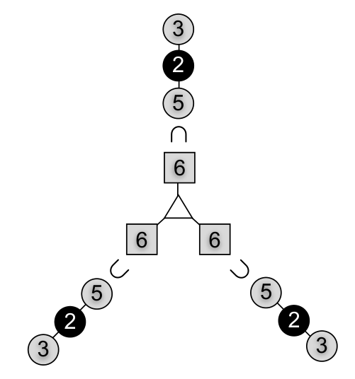
Here, a $SO(2N-1)$ gauge group in each tail is gauging the subgroup of $SO(2N)$ flavor symmetry associated with $\odot$ on the sphere. The sphere with three $\odot$ expresses a theory with $SO(2N)^{3}$ flavor symmetry and no marginal gauge coupling. This theory is denoted by $T_{SO(2N)}$ in [4].⁵⁵ 5 This is the $SO(2N)$ counterpart of $T_{N}$ theory studied in [1]. We can determine the anomalies $a$ and $c$ of $T_{SO(2N)}$ theory so that the total anomaly of the quiver is the same as that of the original linear quiver with gauge group (2.6). Following [2], we define $n_{v}$ and $n_{h}$ for $T_{SO(2N)}$ theory so that its conformal anomalies $a$ and $c$ are written as

The explicit expression for $n_{v}$ and $n_{h}$ of $T_{SO(2N)}$ theory was calculated in [4] as

We can also consider a theory with $SO(2N)\times USp(2N-2)^{2}$ flavor symmetry without any marginal coupling, which we denote by $\widetilde{T}_{SO(2N)}$. Such a theory is constructed by considering a linear quiver of $6N-7$ gauge groups

whose G-curve is a sphere with $6N-4$ punctures of $\times$ (See figure 4). We now deform this curve so that it has a single tail with $2N-2$ punctures of $\times$ and two tails with $2N-1$ punctures of $\times$.

The former tail describes the the linear quiver with gauge groups (2.7). On the other hand, each of the latter tails involves a linear quiver with gauge groups

The three tails are connected to a sphere with a puncture of $\odot$ and two punctures of $\star$, which implies that the sphere describes $\widetilde{T}_{SO(2N)}$ theory. We can calculate $n_{v}$ and $n_{h}$ for this $\widetilde{T}_{SO(2N)}$ theory, exactly in the same way as for $T_{SO(2N)}$. The result is

Note that there is no similar theory with $USp(2N-2)^{3}$ or $SO(2N)^{2}\times USp(2N-2)$ flavor symmetry because the puncture $\star$ has a non-trivial $\mathbb{Z}_{2}$ monodromy around it [4].

Furthermore, we can also consider a Riemann surface of genus $g>0$ as a G-curve. Then, the low energy gauge theory is described by $2N$ M5-branes wrapping on the Riemann surface of genus $g$, which is not S-dual to any linear quiver theory. In general, theories which are related to each other by S-duality have the same punctures and genus of the G-curve. In the next section, we will consider the gravity dual of $SO/USp$ quivers whose G-curve has no puncture. The dual gravity for various $SO/USp$-type tails is studied in section 4.

The gravity duals of $SU(M)$ quivers that arise as the low energy theories of $M$ M5-branes on a Riemann surface was studied in [2]. In particular, when the Riemann surface has genus $g>1$ and no puncture, the near-horizon geometry of the M5-branes is identified with $AdS_{5}\times\Sigma_{g}\times S^{4}$, where $S^{4}$ is non-trivially fibered over the Riemann surface $\Sigma_{g}$. The corresponding eleven-dimensional metric is given by

where $W\equiv 1+\cos^{2}\theta$. The parameters $\theta,\psi,\phi$ and $\chi$ are the coordinates on $S^{4}$, while $r$ and $\beta$ parameterize a hyperbolic space. We obtain a Riemann surface by considering a quotient of the hyperbolic space by some group $\Gamma$. This metric has a symmetry $SU(2)\times U(1)$ which is suitable for the gravity dual of $d=4,\mathcal{N}=2$ theories. From the above metric, the conformal anomaly $c$ of the four-dimensional gauge theory is holographically evaluated as [20, 2]

where $G_{\rm N}^{d}$ is $d$-dimensional Newtonian constant and $R_{AdS_{5}}$ is the curvature radius of the $AdS_{5}$.

The result (3.2) in the gravity side matches with the field theory calculation. The field theory whose G-curve is a Riemann surface of genus $g$ without punctures is described by a quiver diagram as in figure 5, which involves mysterious $T_{M}$ theories with $SU(M)^{3}$ flavor symmetry and no marginal coupling [1].

The anomaly contributions $n_{v}$ and $n_{h}$ of $T_{M}$ theory can be read off via S-duality invariance [2], which leads to the following total contributions from the whole quiver:

Then the total anomaly coefficient $c$ is evaluated in the field theory side as

which agrees with the gravity side calculation (3.2) in the large $M$ limit. In [2], it was also shown that subleading contributions in (3.3) are also consistent with the anomaly polynomial of the six-dimensional $(2,0)$ theory which was calculated by considering the anomaly inflow from the bulk [21].

We now generalize the above argument to the $SO/USp$ superconformal quivers. The main difference from the $SU$-type quivers is the presence of a $\mathbb{Z}_{2}$-quotient. Namely, we consider $2N$ M5-branes on top of $\mathbb{R}^{5}/\mathbb{Z}_{2}$ which are wrapping on a Riemann surface of genus $g$ without punctures. From table 1 and table 2, we find that such a configuration gives D4-branes with O4^±-plane in the type IIA limit, which lead to $SO(2N),USp(2N-2)$ gauge groups in four dimensions. The $\mathbb{Z}_{2}$-quotient only affects $\mathbb{R}^{5}$ spanned by $x^{4,5,7,8,9}$, which replaces the $S^{4}$ surrounding M5-branes with $\mathbb{RP}^{4}$. Then, the corresponding gravity dual is described by the same metric (3.1) with $M=2N$ but now $\theta,\psi,\phi$ and $\chi$ parameterize $\mathbb{RP}^{4}$ rather than $S^{4}$.

As a $SO/USp$ superconformal quiver gauge theory whose G-curve is a Riemann surface of genus $g$ without punctures, we can consider a theory described by a quiver diagram depicted in figure 6.

It involves $(3g-3)$ $SO(2N)$ gauge groups and $(2g-2)$ $T_{SO(2N)}$ theories, and therefore the total contributions to $n_{v}$ and $n_{h}$ are

Then the conformal anomaly $c$ of the quiver gauge theory is evaluated as

On the other hand, the holographic calculation from the gravity dual gives

which agrees with (3.7) in the large $N$ limit. This supports the validity of (2.9) in the large $N$ limit, which was calculated via the S-duality invariance of the four-dimensional field theory.

For completeness, we here describe that the subleading terms in (3.5) and (3.6) are consistent with the anomaly polynomial of the six-dimensional field theory. A field theory on $2N$ M5-branes on top of $\mathbb{R}^{5}/\mathbb{Z}_{2}$ is the $D_{N}$-type $(2,0)$ theory. The anomaly polynomial of the theory is evaluated in [22] so that the anomaly coming from the polynomial is canceled by the anomaly inflow through the Chern-Simons coupling in eleven-dimensional gravity. The explicit expression for the anomaly eight-form is

where $p_{i}(\mathcal{B})$ is the $i$-th Pontryagin class of a bundle $\mathcal{B}$, and $\mathcal{N}$ is the normal bundle of the M5-brane world-volume. The eight-form $\mathcal{J}_{8}$ is the one-loop anomaly polynomial of a single $(2,0)$ tensor multiplet:

where $\mathcal{T}$ is the tangent bundle of the world-volume.

By integrating this $I_{8}$ along the Riemann surface, we can obtain the anomaly six-form $I_{6}$ of the four-dimensional theory. The anomaly coefficients of $I_{6}$ give R-symmetry anomalies in four dimensions, which are related to the conformal anomalies via superconformal symmetry. Therefore, we can read off $a$ and $c$ from the anomaly coefficients of $I_{6}$. In fact, such a calculation was carried out in the appendix of [23], which tells us that the resulting conformal anomalies are written as

By using (2.8), we can then read off $n_{v}$ and $n_{h}$ of the quiver gauge theory, which perfectly agree with (3.5) and (3.6).⁶⁶ 6 For some interesting observations on the anomaly polynomials of the $(2,0)$ theory in related topics, see [24, 25, 26].

We have other four-dimensional quiver gauge theories whose G-curve is the same $\Sigma_{g}$. For example, let us consider the simplest case $g=2$. In this case, we have previously considered the theory with three $SO(2N)$ gauge groups and two $T_{SO(2N)}$ theories. However, we can also consider a theory with two $USp(2N-2)$ and a single $SO(2N)$ gauge groups together with two $\widetilde{T}_{SO(2N)}$ theories, whose quiver diagram is shown in the right picture of figure 7.

The latter theory has two $USp(2N-2)$ gauge groups instead of $SO(2N)$. Recall that the M-theory lifts of $SO(2N)$ and $USp(2N-2)$ gauge theories for $\varphi=0$ are both given by $2N$ M5-branes on $\mathbb{R}^{5}\times\mathbb{R}^{5}/\mathbb{Z}_{2}\times S^{1}$. The only difference is that two of $2N$ M5-branes are localized at the $\mathbb{Z}_{2}$ fixed plane for $USp(2N-2)$ gauge theory. This “freezing” of two M5-branes is due to the non-vanishing torsion part of the four-form flux [11].

Since the torsion element of the four-form flux can be expressed by a flat three-form potential, we expect that such a torsion part does not affect the anomaly eight-form (3.9) evaluated by the anomaly inflow method. If this is the case, the two theories in figure 7 have the same conformal anomalies. In order to verify this, we calculate $n_{v}$ and $n_{h}$ for the right quiver of figure 7. By using the expressions (2.12) for the anomalies of the $\widetilde{T}_{SO(2N)}$, the total contributions to $n_{v}$ and $n_{h}$ are evaluated as

which are exactly the same as (3.5) and (3.6) for $g=2$. This strongly suggests that the two quiver gauge theories associated with the two quiver diagrams in figure 7 share the same metric of the dual gravity as studied in the previous subsection.

We can generalize the above argument on the conformal anomalies to theories with $\Sigma_{g}$ for $g>2$. Let us consider an arbitrary superconformal which is constructed from $SO(2N)$ and $USp(2N-2)$ gauge groups, $T_{SO(2N)}$ theories, and $\widetilde{T}_{SO(2N)}$ theories. An example is shown in figure 8.

Any such quiver can be obtained by replacing some $SO(2N)$ and $T_{SO(2N)}$ with $USp(2N-2)$ and $\widetilde{T}_{SO(2N)}$ in a quiver of figure 6. Since the $\widetilde{T}_{SO(2N)}$ theory has $SO(2N)\times USp(2N-2)^{2}$ flavor symmetry, such a replacement should be realized by repeating primitive replacements defined below.

The primitive replacement is defined as a replacement of a closed chain of $SO(2N)$ gauge groups and $T_{SO(2N)}$ theories of the form

$\displaystyle\parbox{426.79134pt}{\hbox{\includegraphics[width=426.79134pt]{chain_SO.pdf}}},$

with the following closed chain of $USp(2N-2)$ gauge groups and $\widetilde{T}_{SO(2N)}$ theories:

$\displaystyle\parbox{426.79134pt}{\hbox{\includegraphics[width=426.79134pt]{chain_USp.pdf}}}.$

Here the leftmost and rightmost gauge groups in each chain are identified. Since the original chain has equal numbers, say $k$, of $SO(2N)$ gauge groups and $T_{\rm SO(2N)}$ theories, the primitive replacement replaces $k$ $SO(2N)$ with $k$ $USp(2N-2)$ as well as $k$ $T_{SO(2N)}$ with $k$ $\widetilde{T}_{SO(2N)}$. What is important here is that this replacement keeps $n_{v}$ and $n_{h}$ invariant, which follows from

Since any quiver which only involves $SO/USp$ gauge groups and $T_{SO},\widetilde{T}_{SO}$ theories can be obtained by repeating the primitive replacements in a quiver of figure 6, it has the same $n_{v}$ and $n_{h}$ as (3.5) and (3.6). Hence, if a $SO/USp$ superconformal quiver has a G-curve $\Sigma_{g}$ without punctures, then its conformal anomalies are determined only by the genus $g$ of the G-curve and independent of the choice of gauge groups associated with the handles of $\Sigma_{g}$. This particularly suggests that they share the same metric of the dual gravity as the one studied in subsection 3.2. In the next subsection, we see how we can distinguish the gravity duals of such theories with the same G-curve $\Sigma_{g}$.

We have seen that there are several quiver gauge theories which have the same G-curve $\Sigma_{g}$ and the same anomaly contributions $n_{v},n_{h}$. In fact, such theories are further classified by the torsion part of the four-form flux in M-theory.⁷⁷ 7 The author thanks Yuji Tachikawa for pointing out this fact.

Let us first consider M5-branes on $\mathbb{R}^{5}\times\mathbb{R}^{5}/\mathbb{Z}_{2}\times S^{1}$. Since the spacetime (from which the M5-brane locus is removed) is contractible to $\mathbb{RP}^{4}\times S^{1}$, the topology of the three-form potential is measured by $H^{4}(\mathbb{RP}^{4}\times S^{1},\widetilde{\mathbb{Z}})$.⁸⁸ 8 Note here that, since the $\mathbb{Z}_{2}$-fixed plane carries M5 charge $-1$ (counted in the covering space), the four-form flux $[G_{4}/2\pi]$ itself is not a cohomology class in $H^{4}(\mathbb{RP}^{4}\times S^{1},\widetilde{\mathbb{Z}})$ [11]. To make an element of $H^{4}(\mathbb{RP}^{4}\times S^{1},\widetilde{\mathbb{Z}})$, we need to define a modified cohomology class $[\widetilde{G}_{4}/2\pi]\equiv\frac{1}{2}([G_{4}/\pi]-\chi_{\rm E})\in H^{4}(\mathbb{RP}^{4}\times S^{1},\widetilde{\mathbb{Z}})$, where $\chi_{\rm E}$ denotes the twisted Euler class. Then, the $H$-flux in type IIA limit is obtained by $\int_{S^{1}}[\widetilde{G}_{4}/2\pi]=[H/2\pi]\in H^{3}(\mathbb{RP}^{4},\widetilde{\mathbb{Z}})$. For more detail, see the appendix of [11]. As discussed in [11], the cohomology group $H^{4}(\mathbb{RP}^{4}\times S^{1},\widetilde{\mathbb{Z}})$ includes two-torsion:

where the integrations over $\mathbb{RP}^{4}$ and $S^{1}$ induce projections $H^{4}(\mathbb{RP}^{4}\times S^{1},\widetilde{\mathbb{Z}})\to\mathbb{Z}$ and $H^{4}(\mathbb{RP}^{4}\times S^{1},\widetilde{\mathbb{Z}})\to\mathbb{Z}_{2}$, respectively. This means that the first $\mathbb{Z}$ in (3.17) counts the number of M5-branes wrapping on $\mathbb{R}^{5}\times S^{1}$, while the torsion part $\mathbb{Z}_{2}$ can be identified with $H^{3}(\mathbb{RP}^{4},\widetilde{\mathbb{Z}})$ which measures the topology of NSNS $B$-field in the type IIA limit. In particular, the phase $\vartheta$ defined in (2.1) is equivalent to the integral of the four-form flux along $S^{1}\times\mathbb{RP}^{3}$.⁹⁹ 9 Since the flux is a twisted four-form and $\mathbb{RP}^{3}\times S^{1}$ is an untwisted cycle, this integral is well-defined as an element of $\mathbb{Z}_{2}$. Thus, the difference between O4⁺ and O4^--planes is lifted to a difference in the torsion part $\mathbb{Z}_{2}$.

Now, let us consider two types of “pairs of pants” in the G-curve as in figure 9, which correspond to the M-theory lifts of $T_{SO}$ and $\widetilde{T}_{SO}$-theories, respectively.

Each type of the pants has three tubes attached to it, and each such tube is associated with a one-cycle $S^{1}_{(i)}$ for $i=1,2,3$ with the orientation as in figure 9. The torsion part of the four-form flux associated to the $i$-th tube is measured by integrating the flux along $S^{1}_{(i)}\times\mathbb{RP}^{3}$. We denote such integral of the flux by $\vartheta_{i}$ for the $i$-th tube.¹⁰¹⁰ 10 For the same reason as before, this flux is the modified flux $[\widetilde{G}_{4}/2\pi]$. To be more specific, $\vartheta_{i}=\int_{S^{1}_{(i)}\times\mathbb{RP}^{4}}[\widetilde{G}_{4}/2\pi]$. The left and right examples in figure 9 have $(\vartheta_{1},\vartheta_{2},\vartheta_{3})=(0,0,0)$ and $(1,1,0)$, respectively. Since $\vartheta_{i}\in\mathbb{Z}_{2}$, one might think that a single pair of pants generally has four possibilities of $(\vartheta_{1},\vartheta_{2},\vartheta_{3})$ up to permutation. However, the fact $\sum_{i}S^{1}_{(i)}=0$ implies that

as an element of $\mathbb{Z}_{2}$, which forbids $(\vartheta_{1},\vartheta_{2},\vartheta_{3})=(1,0,0),\,(1,1,1)$. This is consistent with the absence of the four-dimensional theory which has $SO(2N)^{2}\times USp(2N-2)$ or $USp(2N-2)^{3}$ flavor symmetry and no marginal coupling.

The non-trivial torsion part of the four-form flux can be expressed by drawing a red line through tubes with $\vartheta_{i}\neq 0$, as in figure 9. Due to the absence of the pair of pants which has $SO(2N)^{2}\times USp(2N-2)$ or $USp(2N-2)^{3}$ flavor symmetry, such a red line should form a closed curve (figure 10). This particularly implies that the non-vanishing torsion part of the four-form flux is associated to one-cycles of the G-curve which are transverse to the M-theory circle, as long as the curve has no punctures.

References

- [1] D. Gaiotto, “N=2 dualities,” arXiv:0904.2715 [hep-th].
- [2] D. Gaiotto and J. Maldacena, “The Gravity duals of N=2 superconformal field theories,” arXiv:0904.4466 [hep-th].
- [3] J. M. Maldacena and C. Nunez, “Supergravity description of field theories on curved manifolds and a no go theorem,” Int. J. Mod. Phys. A 16 (2001) 822 [hep-th/0007018].
- [4] Y. Tachikawa, “Six-dimensional D(N) theory and four-dimensional SO-USp quivers,” JHEP 0907, 067 (2009) [arXiv:0905.4074 [hep-th]].
- [5] F. Benini, Y. Tachikawa and D. Xie, “Mirrors of 3d Sicilian theories,” JHEP 1009 (2010) 063 [arXiv:1007.0992 [hep-th]].
- [6] Y. Tachikawa, “N=2 S-duality via Outer-automorphism Twists,” J. Phys. A A 44 (2011) 182001 [arXiv:1009.0339 [hep-th]].
- [7] D. Nanopoulos and D. Xie, “More Three Dimensional Mirror Pairs,” JHEP 1105 (2011) 071 [arXiv:1011.1911 [hep-th]].
- [8] L. Hollands, C. A. Keller and J. Song, “From SO/Sp instantons to W-algebra blocks,” JHEP 1103 (2011) 053 [arXiv:1012.4468 [hep-th]].
- [9] O. Chacaltana and J. Distler, “Tinkertoys for the series,” arXiv:1106.5410 [hep-th].
- [10] L. Hollands, C. A. Keller and J. Song, “Towards a 4d/2d correspondence for Sicilian quivers,” JHEP 1110 (2011) 100 [arXiv:1107.0973 [hep-th]].
- [11] K. Hori, “Consistency Condition for Fivebrane in M theory on Orbifold,” Nucl. Phys. B 539 (1999) 35 [hep-th/9805141].
- [12] N. J. Evans, C. V. Johnson and A. D. Shapere, “Orientifolds, branes, and duality of 4-D gauge theories,” Nucl. Phys. B 505 (1997) 251 [hep-th/9703210].
- [13] K. Landsteiner, E. Lopez and D. A. Lowe, “N=2 supersymmetric gauge theories, branes and orientifolds,” Nucl. Phys. B 507 (1997) 197 [hep-th/9705199].
- [14] A. Brandhuber, J. Sonnenschein, S. Theisen and S. Yankielowicz, “M theory and Seiberg-Witten curves: Orthogonal and symplectic groups,” Nucl. Phys. B 504 (1997) 175 [hep-th/9705232].
- [15] J. de Boer, K. Hori, H. Ooguri and Y. Oz, “Branes and dynamical supersymmetry breaking,” Nucl. Phys. B 522 (1998) 20 [hep-th/9801060].
- [16] E. G. Gimon, “On the M theory interpretation of orientifold planes,” hep-th/9806226.
- [17] E. Witten, “Solutions of four-dimensional field theories via M theory,” Nucl. Phys. B 500 (1997) 3 [hep-th/9703166].
- [18] A. Hanany and E. Witten, “Type IIB superstrings, BPS monopoles, and three-dimensional gauge dynamics,” Nucl. Phys. B 492 (1997) 152 [hep-th/9611230].
- [19] D. Gaiotto, G. W. Moore and A. Neitzke, “Wall-crossing, Hitchin Systems, and the WKB Approximation,” arXiv:0907.3987 [hep-th].
- [20] M. Henningson and K. Skenderis, “The Holographic Weyl anomaly,” JHEP 9807 (1998) 023 [hep-th/9806087].
- [21] J. A. Harvey, R. Minasian and G. W. Moore, “NonAbelian tensor multiplet anomalies,” JHEP 9809 (1998) 004 [hep-th/9808060].
- [22] P. Yi, “Anomaly of (2,0) theories,” Phys. Rev. D 64, 106006 (2001) [hep-th/0106165].
- [23] L. F. Alday, F. Benini and Y. Tachikawa, “Liouville/Toda central charges from M5-branes,” Phys. Rev. Lett. 105 (2010) 141601 [arXiv:0909.4776 [hep-th]].
- [24] F. Benini, Y. Tachikawa and B. Wecht, “Sicilian gauge theories and N=1 dualities,” JHEP 1001 (2010) 088 [arXiv:0909.1327 [hep-th]].
- [25] G. Bonelli and A. Tanzini, “Hitchin systems, N=2 gauge theories and W-gravity,” Phys. Lett. B 691 (2010) 111 [arXiv:0909.4031 [hep-th]].
- [26] T. Nishioka and Y. Tachikawa, “Central charges of para-Liouville and Toda theories from M-5-branes,” Phys. Rev. D 84 (2011) 046009 [arXiv:1106.1172 [hep-th]].
- [27] Y. Tachikawa, “On W-algebras and the symmetries of defects of 6d N=(2,0) theory,” JHEP 1103 (2011) 043 [arXiv:1102.0076 [hep-th]].