Magneto-transport in a binary alloy ring

Paramita Dutta Email: paramita.dutta@saha.ac.in Affiliation: Theoretical Condensed Matter Physics Division, Saha Institute of Nuclear Physics, Sector-I, Block-AF, Bidhannagar, Kolkata-700 064, India Santanu K. Maiti Email: santanu@post.tau.ac.il Affiliation: School of Chemistry, Tel Aviv University, Ramat-Aviv, Tel Aviv-69978, Israel S. N. Karmakar Email: sachindranath.karmakar@saha.ac.in Affiliation: Theoretical Condensed Matter Physics Division, Saha Institute of Nuclear Physics, Sector-I, Block-AF, Bidhannagar, Kolkata-700 064, India

Abstract

Magneto-transport properties are investigated in a binary alloy ring subjected to an Aharonov-Bohm (AB) flux $\phi$ within a single-band non-interacting tight-binding framework. In the first part, we expose analytically the behavior of persistent current in an isolated ordere binary alloy ring as functions of electron concentration $N_{e}$ and AB flux $\phi$ . While, in the second part of the article, we discuss electron transport properties through a binary alloy ring attached to two semi-infinite one-dimensional metallic electrodes. The effect of impurities is also analyzed. From our study we propose that under suitable choices of the parameter values the system can act as a $p$ -type or an $n$ -type semiconductor.

Keywords:

Magneto-transport; Wave-guide theory; Persistent current; Binary alloy ring; Semiconducting behavior.

pacs

73.23.-b, 73.23.Ra, 71.23.An

I Introduction

The enormous advancements of nano-science and technology over the last few decades have allowed us to investigate electron transport in low-dimensional model quantum systems in a very tunable way. The precision instruments bestowed by nanotechnology have given indulgence to such low-dimensional systems with tailor-made geometries to become promising candidates for different nano-electronic devices. One of such geometries is a mesoscopic ring which looks very simple but has very high potential from the application perspective. Several quantum mechanical phenomena have been observed in this closed loop structure specially in presence of magnetic flux [1, 2, 3, 4, 5]. The existence of dissipationless current, the so-called persistent current, in a mesoscopic normal metal ring pierced by an AB flux $\phi$ is one of such remarkable effects which reveals the importance of phase coherence of electronic wave functions in low-dimensional systems. In 1983, Büttiker et al. [6] initially predicted this significant phenomenon through some theoretical arguments, but, its actual realization came much later after the nice experiment done by Levy et al. [7]. They have observed the oscillations with period $\phi_{0}/2$ ( $\phi_{0}=ch/e$ , the elementary flux-quantum) while measuring persistent current in an ensemble of $10^{7}$ independent Cu rings. Similar $\phi_{0}/2$ oscillations were also reported not only for an ensemble of disconnected $10^{5}$ Ag rings [8] but also for an array of $10^{5}$ isolated GaAs-AlGaAs rings [9, 10]. Later many other theoretical [11, 12, 13] as well as experimental [14, 15] attempts have also been made to reveal the actual mechanisms of persistent current in single-channel rings and multi-channel cylinders. Similar to persistent current in such isolated closed geometries, the non-decaying charge current is also observed in open systems [16, 17, 18, 19, 20, 21, 22, 23, 24] like, a mesoscopic ring with side attached electrodes.

Though a wealth of literature has already been generated involving the analysis of persistent current in conventional mesoscopic rings, cylinders, connected rings, ring with multi-arm structures, there is still need to look deeper into the problem to address several important issues those have not been explored earlier. In the present article we undertake an in-depth study of magneto-transport through a binary alloy mesoscopic ring in presence of the magnetic flux $\phi$ within a single-band non-interacting tight-binding framework. We analyze our results in two parts. In the first part, we describe the energy band structure and persistent current for an ordered binary alloy ring. We perform these results analytically. In the second part, we describe the magneto-transport properties in presence of external electrodes

Refer to caption — Figure 1: (Color online). A binary alloy ring, threaded by a magnetic flux $\phi$ , is composed of two different types of atomic sites, viz, $\alpha$ and $\beta$ those are represented by filled green and magenta circles, respectively.

which include transmission probabilities, persistent currents and related issues. Quite interestingly we examine that if we include some new additional atomic sites, called as impurities, those are not necessarily to be random, in any part of the binary alloy ring, some quasi-localized energy levels appear depending on the number of impurity sites within the band of extended regions. The positions of these nearly-localized energy levels can also be tuned with respect to the extended regions by means of some external gate voltages. It leads to the possibility of using such a system as a $p$ -type or an $n$ -type semiconductor by fixing the Fermi level at appropriate energy.

In what follows, we describe the model quantum systems and the results. In Section II we present the results and related discussions for an ordered binary alloy ring. Section III illustrates the model and the theoretical approach to calculate transmission probability, persistent current and related issues in presence of external leads, and the numerical results are described in Section IV. Finally, in Section V we draw our conclusions.

II Ordered binary alloy ring without external leads

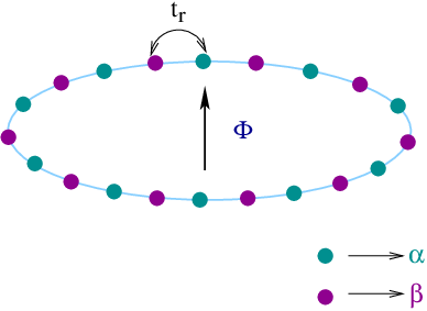
Model: The model quantum system is illustrated schematically in Fig. 1. An ordered binary alloy ring, subjected to an AB flux $\phi$ , composed of two different types of atoms, namely, $\alpha$ and $\beta$ those are placed alternately in a regular pattern. We use a non-interacting single-band tight-binding (TB) Hamiltonian to describe the model quantum of $\alpha$ and $\beta$ sites) binary alloy ring the TB Hamiltonian reads,

H_{R}=\sum_{l}(\epsilon_{l}c^{{\dagger}}_{l}c_{l}+t_{r}e^{i\theta}c^{{\dagger}}_{l}c_{l+1}+t_{r}e^{-i\theta}c^{{\dagger}}_{l+1}c_{l})

(1)

where, $\epsilon_{l}$ is the on-site energy and $t_{r}$ refers to the nearest-neighbor hopping strength. For the site $\alpha$ , $\epsilon_{l}$ is identical to $\epsilon_{\alpha}$ , while it is $\epsilon_{\beta}$ for the site $\beta$ . The phase factor $\theta=2\pi\phi/N$ appears into the Hamiltonian due to the magnetic flux $\phi$ threaded by the ring which is measured by the elementary flux-quantum $\phi_{0}$ . $c_{l}^{\dagger}$ ( $c_{l}$ ) is the creation (annihilation) operator for an electron at the site $l$ .

Energy spectrum: In order to explore the characteristic features of persistent current in an ordered binary alloy ring, let us begin with the energy band structure. We do it analytically. The energy dispersion

relation for the ordered binary alloy ring can be expressed mathematically as,

E=\frac{\epsilon_{\alpha}+\epsilon_{\beta}}{2}\pm\sqrt{\left(\frac{\epsilon_{\alpha}-\epsilon_{\beta}}{2}\right)^{2}+4\,t_{r}^{2}\,cos^{2}{\left(ka\right)}}

(2)

where, $a$ is the lattice spacing and $k$ is the wave vector. In presence of the AB flux $\phi$ , the quantized values of $k$ are obtained from the relation,

k=\frac{2\pi}{Na}\left(n+\frac{\phi}{\phi_{0}}\right)

(3)

where, $n$ is an integer and it is restricted within the range: $-N/2\leq n<N/2$ . As illustrative example, in Fig. 2 we plot the energy levels as a function of flux $\phi$ , obtained from Eq. 2, for a $40$ -site binary alloy ring considering $\epsilon_{\alpha}=-\epsilon_{\beta}=1$ and $t_{r}=1$ . It shows that two different sets of energy levels are obtained, forming two quasi-bands, and they are separated by a finite energy gap. This gap, on the other hand, is tunable by the parameter values describing the TB Hamiltonian Eq. 1. The origin of two different sets of energy levels is also clearly visible from Eq. 2. From the energy spectrum (Fig. 2) we see that at half-integer or integer multiples of flux-quantum, energy levels have either a maximum or a minimum and it results vanishing nature of persistent current at these specific values of $\phi$ , since the current is obtained by taking the first order derivative of energy $E(\phi)$ with

respect to flux $\phi$ [12]. All these energy levels vary periodically providing $\phi_{0}$ flux-quantum periodicity.

Persistent current: Once we get the energy eigenvalues as a function of flux $\phi$ , we can easily calculate persistent current for individual energy eigenstates. It is simply the first order derivative of energy with respect to flux $\phi$ . Therefore, for an $n$ -th energy eigenstate we can write the expression for the current as,

I_{n}=\pm\left(\frac{4\pi t_{r}^{2}}{Na\phi_{0}}\right)\frac{sin{\left[\frac{4\pi}{Na}\left(n+\phi/\phi_{0}\right)\right]}}{\sqrt{1+4t_{r}^{2}cos^{2}{\left[\frac{2\pi}{Na}\left(n+\phi/\phi_{0}\right)\right]}}}

(4)

where, $+$ ve or $-$ ve sign in the current expression appears depending on the choice of $n$ i.e., in which sub-band the energy level exists. At absolute zero temperature, total persistent current $I$ for a particular filling $N_{e}$ is obtained by taking the sum of individual contributions from the lowest $N_{e}$ energy eigenstates. Thus, we can write,

I=\sum_{n=1}^{N_{e}}I_{n}

(5)

As representative examples, in Fig. 3 we display the variation of persistent current for an ordered $120$ -site binary alloy ring considering $\epsilon_{\alpha}=-\epsilon_{\beta}=1$ and $t_{r}=1$ in the different filled band cases. For odd number of electrons the results are shown in Fig. 3(a) while, in Fig. 3(b) the results are given for even number of electrons. Both for the odd and even $N_{e}$ , persistent current shows saw-tooth like variation as a function of flux $\phi$ , similar to that of traditional single-channel mesoscopic rings. The sharp transitions at half-integer (for odd $N_{e}$ ) or integer (for even $N_{e}$ ) multiples of flux-quantum ( $\phi_{0}$ ) in persistent current appears due to the crossing of energy levels at these respective values of $\phi$ . Quite interestingly, we also examine that the current shows always diamagnetic in nature irrespective of the filling factor.

III Binary alloy ring with side-attached leads

In the rest of the present article we explore the essential features of magneto-transport properties for a binary alloy ring in presence of external leads i.e., for an open system.

Model: The model quantum system is depicted in Fig. 4 where a binary alloy ring, threaded by a magnetic flux $\phi$ , is attached to two semi-infinite one-dimensional metallic electrodes. The ring is composed of $N_{1}$ identical pairs of $\alpha$ - $\beta$ sites and $N_{2}$ identical foreign atomic sites, labeled as $\gamma$ sites, those are embedded in a small portion of the ring. These sites ( $\gamma$ sites) are often called as impurity sites. We label the atomic sites of two side-attached leads in a particular way, as shown in Fig. 4, and they are connected to the ring via the sites $\mu$ and $\nu$ . A single-band non-interacting tight-binding framework is used to describe the entire system. For the full system we can write the total Hamiltonian as a sum of three terms like,

H=H_{R}+H_{L}+H_{T}

(6)

where, $H_{R}$ , $H_{L}$ and $H_{T}$ correspond to the Hamiltonians for the ring, leads (left and right) and tunneling between the ring and leads, respectively. The first term ( $H_{R}$ ) looks exactly similar as in Eq. 1, but here $\epsilon_{l}$ has three possibilities for three different atomic sites ( $\alpha$ , $\beta$ and $\gamma$ ). We can also tune the site energy $\epsilon_{\gamma}$ by means of some external gate voltage $V_{g}$ , and thus, we can write it as $\epsilon_{\gamma}=\epsilon_{\gamma}^{0}+V_{g}$ , where $\epsilon_{\gamma}^{0}$ is the site energy in absence of any external potential. The other two terms of Eq. 6, $H_{L}$ and $H_{T}$ , can also be expressed in a similar fashion as,

H_{L}=\underbrace{t_{0}\sum_{m\leq 0}\left(b_{m}^{{\dagger}}b_{m-1}+h.c.\right)}_{\mbox{left lead}}+\underbrace{t_{0}\sum_{m\geq 1}\left(b_{m}^{{\dagger}}b_{m+1}+h.c.\right)}_{\mbox{right lead}}

(7)

and,

H_{T}=\left(\tau_{L}b_{0}^{{\dagger}}c_{\mu}+\tau_{R}b_{1}^{{\dagger}}c_{\nu}\right)+h.c.

(8)

The site energy dependent term in $H_{L}$ is omitted as we set the site energy for the identical sites in the leads to zero. $b_{m}^{{\dagger}}$ ( $b_{m}$ )

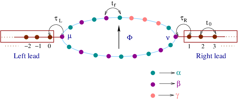
corresponds to the creation (annihilation) operator of an electron at the site $m$ of the leads and $t_{0}$ represents the nearest-neighbor hopping integral in these leads. $\tau_{L}$ is the coupling strength between the left lead and the ring, while it is $\tau_{R}$ for the other case.

Wave-guide theory: To find transmission probability across the ring and also to calculate persistent current in such an open ring system we adopt wave-guide theory [18, 21, 22]. Here we describe it very briefly.

Let us start with the Scrödinger equation $H|\psi\rangle=E|\psi\rangle$ , where $|\psi\rangle$ is the stationary wave function of the entire system. In the Wannier basis it ( $|\psi\rangle$ ) can be written as,

|\psi\rangle=\underbrace{\sum_{m\leq 0}B_{m}|m\rangle}_{\mbox{left lead}}+\underbrace{\sum_{m\geq 1}B_{m}|m\rangle}_{\mbox{right lead}}+\underbrace{\sum_{l}C_{l}|l\rangle}_{\mbox{ring}}

(9)

where, the co-efficients $B_{m}$ and $C_{l}$ correspond to the probability amplitudes in the respective sites. Assuming that the electrons are described by a plane wave we can express the wave amplitudes in the left and right leads as,

B_{m}=e^{ikm}+re^{-ikm},\hskip 8.5359pt{\mbox{for}}\hskip 8.5359ptm\leq 0

(10)

and

B_{m}=te^{ikm},\hskip 8.5359pt{\mbox{for}}\hskip 8.5359ptm\geq 1

(11)

where, $r$ and $t$ are the reflection and transmission amplitudes, respectively. $k$ is the wave number and it is related to the energy $E$ of the incident electron by the expression $E=2t_{0}\cos{k}$ . The lattice spacing $a$ is set equal to $1$ .

Now to find out the transmission amplitude $t$ , we have to solve the following set of coupled linear equations.

$\displaystyle EB_{0}$	$\displaystyle=$	$\displaystyle t_{0}B_{-1}+\tau_{L}C_{\mu}$
$\displaystyle(E-\epsilon_{l})C_{l}$	$\displaystyle=$	$\displaystyle t_{r}e^{i\phi}C_{l+1}+t_{r}e^{-i\phi}C_{l-1}+\tau_{L}B_{0}\delta_{l,\mu}$
		$\displaystyle~~~~~~~~~~~~+\tau_{R}B_{1}\delta_{l,\nu}$
$\displaystyle EB_{1}$	$\displaystyle=$	$\displaystyle t_{0}B_{2}+\tau_{R}C_{\nu}$	(12)

where, the co-efficients $B_{0}$ , $B_{-1}$ , $B_{1}$ and $B_{2}$ can be easily expressed in terms of $r$ and $t$ by using Eqs. 10 and 11, and they are in the form:

$\displaystyle B_{0}$	$\displaystyle=$	$\displaystyle 1+r$
$\displaystyle B_{-1}$	$\displaystyle=$	$\displaystyle B_{0}e^{ik}-2i\sin{k}$
$\displaystyle B_{1}$	$\displaystyle=$	$\displaystyle te^{ik}$
$\displaystyle B_{2}$	$\displaystyle=$	$\displaystyle te^{2ik}$	(13)

Thus, for a particular value of $E$ we can easily solve the set of linear equations and find the value of $t$ . Finally, the transmission probability across the ring becomes

T(E)=|t|^{2}

(14)

Now, to calculate persistent current between any two neighboring sites in the ring we use the following relation,

I_{l,l+1}=\frac{2et_{r}}{N\hbar}{\mbox{Im}}\left(C_{l}^{{\dagger}}C_{l+1}e^{-i\phi}\right).

(15)

IV Numerical Results and discussion

Throughout the calculations we set $\epsilon_{\alpha}=-\epsilon_{\beta}=1$ , $\epsilon_{\gamma}^{0}=0$ , $t_{r}=1$ , $\epsilon_{0}=0$ and $t_{0}=2$ . The energy scale is measured in unit of $t_{r}$ and we choose the units where $c=h=e=1$ .

IV.1 Transmission and ADOS spectra

In Fig. 5 we show the variation of transmission probability $T$ (red color) as a function of injecting electron energy $E$ for some typical binary alloy rings considering different number of impurity sites. The average density of states (ADOS) is also superimposed in each spectrum. Here, we fix $N_{1}=28$ and take three different values of $N_{2}$ those are presented in Figs. 5(a), (b) and (c), respectively. In all these cases the magnetic flux $\phi$ is set equal to zero. The results are quite interesting and important also. It is observed that in absence of impurity sites electron can transmit through the ring for two wide band of energies (see Fig. 5(a)). This transmission spectrum exactly overlaps with the ADOS profile ( $\rho$ - $E$ spectrum) which ensures that electronic transmission takes place through all the energy eigenstates of the binary alloy ring and they are extended in nature.

The band splitting for the ordered binary alloy ring is easily understood from our previous discussion (Sec. II) and the gap between these two bands are also tunable by the parameter values describing the system. The situation becomes really interesting when some additional impurities ( $\gamma$ sites) are introduced in any part of the binary alloy ring. Due to the inclusion of such atomic sites some energy levels appear within the band of extended regions those are no longer extended, but they are almost quasi-localized and do not contribute to the electronic transmission. This behavior is well explained in Figs. 5(b) and (c), where $T$ - $E$ and $\rho$ - $E$ spectra are superimposed with each other for two different numbers of impurity sites ( $N_{2}$ ). The transmission of electrons takes place mainly along the two band edges, while in the band centre, several energy levels are there which provide zero transmission probability. The number of these almost localized energy levels between the extended regions gets increased with the increase of impurity sites, and for large enough impurity sites they almost form a quasi-energy band of localized states. The location of the almost localized energy band can be shifted towards the edge of extended

regions simply by tuning the site energy of these foreign atoms, and here we do it by means of applying an external gate voltage $V_{g}$ . This phenomenon can be utilized to use such a geometry as a $p$ -type or an $n$ -type semiconductor by fixing the Fermi level in an appropriate place. To explore this fact in Fig. 6 we present the variation of transmission probability in addition to the ADOS for a much larger ring size where we consider $60$ identical pairs of $\alpha$ - $\beta$ sites and $44$ impurity sites. Two different cases are considered, one for the case when $\epsilon_{\gamma}$ is set at $0.6$ (Fig. 6(a)), and the other is shown for $\epsilon_{\gamma}=-0.6$ (Fig. 6(b)). For a quite large number of impurity sites we get almost quasi-energy bands (ADOS spectra) and quite nicely we see that when $\epsilon_{\gamma}$ is fixed at $0.6$ , a localized energy band for a wide range of energy is formed along the left edge of the extended region (Fig. 6(a)). Now if we choose the Fermi level around $E=-1.7$ , then many electrons in the localized region below the Fermi level can jump, even at much low temperature since the energy gap is almost zero, to the extended regions and can contribute to the current. Thus, we get a large number of excess electrons, depending on the localized energy levels and also the available extended energy states, in the conduction region which behave as n-type carriers. An exactly opposite behavior is obtained when we set $\epsilon_{\gamma}$ to $-0.6$ . In this case the wide band of localized states is formed in the right edge of the extended region

(see Fig. 6(b)). Therefore, if we set the Fermi energy level around $E=1.7$ , then the electrons from the filled extended levels below the Fermi level hop to the nearly empty localized levels, and these electrons do not contribute anything to the current. But some holes are formed in the extended regions which can carry current and we get $p$ -type carriers. So, in short, we can emphasize that by fixing the Fermi level in appropriate places the geometry can be utilized as a $p$ -type or an $n$ -type semiconductor.

Before we end this analysis, we would like to point out that here we present the results for a particular set of parameter values and establish how such a geometry can be utilized as a $p$ -type or an $n$ -type semiconductor upon the movement of the Fermi level. For a model calculation we choose some specific values of the parameters used in the numerical calculation, but all these physical phenomena are exactly invariant with the change of the parameter values. Only the numerical values will be altered. These features are also exactly valid even for a non-zero value of magnetic flux $\phi$ . The physical picture will be much more appealing if we consider larger rings with more impurity sites and it gives us the confidence to propose an experiment in this line. In a recent work Bellucci et al. [24] have done a detailed study of magneto-transport properties in quantum rings considering tunnel barriers in the presence of magnetic field and established how metal-to-insulator transition takes place in such a geometry. It has been shown that by controlling the strength and the positions of the barriers, the energy shift can be done in a tunable way and they have also proposed this model for experimental realization. This is quite analogous to our present study, and therefore, an experiment in this regard will be challenging.

IV.2 Persistent current

The behavior persistent current $I_{U}$ as a function of energy $E$ in the upper arm of an ordered binary alloy ring is presented in Fig. 7, where (a) and (b) correspond to $\phi=0$ and $\phi_{0}/4$ , respectively. The ring is symmetrically coupled to the side attached leads i.e., the upper and lower arms have identical length, and accordingly, the

current $I_{L}$ in the lower arm becomes exactly identical to the current obtained in the upper arm. From the spectra we observe that the current is available for two wide range of energies, separated by a finite gap, associated with the energy levels of the ring those are clearly visible from the ADOS profiles (red color). All these energy eigenstates are extended in nature since they provide a non-zero current, but the nature of the current is quite different for the two different cases i.e., when $\phi=0$ (Fig. 7(a)) and $\phi\neq 0$ (Fig. 7(b)). For $\phi=0$ , persistent current shows $+$ ve value for all the energy levels which predicts that the currents are in the same phase. While, for a finite value of $\phi$ , the phase of the current changes alternatively. So by measuring persistent current we can directly estimate the nature of the current i.e., whether it is paramagnetic or diamagnetic in nature and also predict the characteristics of energy eigenstates, which are somewhat interesting in the study of electron transport.

To explore the effect of impurities on persistent current in such a geometry, in Fig. 8, we display the results for a typical binary alloy ring ( $N_{1}=16$ ) in presence of some impurity sites ( $N_{2}=12$ ), where (a) and (b) represent the results for the upper and lower arms of the ring, respectively. The impurity sites are added in the upper arm of the ring. With the inclusion of impurity sites, the symmetry between the two arms is broken, and therefore, the currents in the upper and lower arms are no longer identical to each other as shown from the spectra (Figs. 8(a) and (b)). Unlike to the ordered binary alloy ring (Fig. 7), here all the energy eigenstates are not extended in nature. Some localized energy levels appear in the band of extended energy states due to the presence of impurity sites in the ring. This is clearly visible from the spectra since for these impurity levels no current is available. Thus, be calculating persistent current we can emphasize the nature of energy eigenstates very nicely, and this idea can be utilized to reveal the localization properties of energy eigenstates in any complicated geometry.

Analogous to our present model, few works [24, 25] have also been done very recently in some mesoscopic rings in presence of tunnel barriers or in presence of an artificial crystal. The nature of energy band structures and the behavior of persistent currents have been described in detail in these samples, and, we hope our results provide some extensions in this regard.

V Conclusion

In the present article we make a detailed study of magneto-transport through a binary alloy ring in presence of magnetic flux $\phi$ within a single-band non-interacting tight-binding framework. The essential results are analyzed in two parts. In the first part, we discuss the band structure and persistent current of an isolated ordered binary alloy ring. These results are done analytically. In the other part, we explore the magneto-transport properties of a binary alloy ring in presence of external leads. The effect of impurities are also addressed. Quite interestingly we see that in presence of some foreign atoms, those are not necessarily be random, in any part of the ring, some quasi-localized energy levels appear within the band of extended energy levels. The locations of these almost localized energy levels can also be regulated by means of some external gate voltage. This leads to a possibility of using such a system as a $p$ -type or an $n$ -type semiconductor by fixing the Fermi level in appropriate places.

References

[1] A. L. Yeyati and M. Buttiker, Phys. Rev. B 52, R14360 (1995).
[2] E. Buks, R. Schuster, M. Heiblum, D. Mahalu, V. Umansky, and H. Shtrikman, Phys. Rev. Lett. 77, 4664 (1996).
[3] S. Jana and A. Chakrabarti, Phys. Rev. B 77, 155310 (2008).
[4] S. Jana and A. Chakrabarti, Phys. Satus Solidi (b) 248, 725 (2011).
[5] P. Dutta, S. K. Maiti, and S. N. Karmakar, Solid State Commun. 150, 1056 (2010).
[6] M. Büttiker, Y. Imry, and R. Landauer, Phys. Lett. A 96, 365 (1983).
[7] L. P. Levy, G. Dolan, J. Dunsmuir, and H. Bouchiat, Phys. Rev. Lett. 64, 2074 (1990).
[8] R. Deblock, R. Bel, B. Reulet, H. Bouchiat, and D. Mailly, Phys. Rev. Lett. 89, 206803 (2002).
[9] B. Reulet, M. Ramin, H. Bouchiat, and D. Mailly, Phys. Rev. Lett. 75, 124 (1995).
[10] H. F. Cheung, Y. Gefen, E. K. Reidel, and W. H. Shih, Phys. Rev. B 37, 6050 (1988).
[11] P. Dutta, S. K. Maiti, and S. N. Karmakar, Eur. Phys. J. B (in press).
[12] S. K. Maiti, M. Dey, S. Sil, A. Chakrabarti, and S. N. Karmakar, Europhys. Lett. 95, 57008 (2011).
[13] S. K. Maiti, Solid State Commun. 150, 2212 (2010).
[14] D. Mailly, C. Chapelier, and A. Benoit, Phys. Rev. Lett. 70, 2020 (1993).
[15] H. Bluhm, N. C. Koshnick, J. A. Bert, M. E. Huber, and K. A. Moler, Phys. Rev. Lett. 102, 136802 (2009).
[16] M. Büttiker, Phys. Rev. B 32, R1846 (1985).
[17] E. Akkermans, A. Auerbach, J. E. Avron, and B. Shapiro, Phys. Rev. Lett. 66, 76 (1991).
[18] J.-B. Xia, Phys. Rev. B 45, 3593 (1992).
[19] P. A. Mello, Phys. Rev. B 47, 16358 (1993).
[20] P. A. Orellana, M. L. Ladrón de Guevra, M. Pacheco, and A. Latgé, Phys. Rev. B 68, 195321 (2003).
[21] A. M. Jayannavar and P. Singha Deo, Phys. Rev B 49, 13685 (1994).
[22] Y.-J. Xiong and X.-T. Liang, Phys. Lett. A 330, 307 (2004).
[23] T. P. Pareek, P. Singha Deo, and A. M. Jayannavar, Phys. Rev. b 52, 14657 (1995).
[24] S. Bellucci and P. Onorato, Physica E 41, 1393 (2009).
[25] S. Bellucci and P. Onorato, Eur. Phys. J. B 73, 215 (2010).