Thrust distribution resummation in $e^{+}e^{-}$ collisions.

Factorisation properties of event-shapes have been widely studied in the literature [34, 35, 36]. Referring to Fig. 1 we recast the cross section (6) as

	$\displaystyle R_{T}(\tau)=\,\,H\left(\frac{Q}{\mu},\alpha_{s}(\mu)\right)$	$\displaystyle\int dk^{2}d\bar{k}^{2}\mathcal{J}\left(\frac{k}{\mu},\alpha_{s}(\mu)\right)\mathcal{\bar{J}}\left(\frac{\bar{k}}{\mu},\alpha_{s}(\mu)\right)$
	$\displaystyle\times$	$\displaystyle\int dw\mathcal{S}\left(\frac{w}{\mu},\alpha_{s}(\mu)\right)\Theta(Q^{2}\tau-\bar{k}^{2}-k^{2}-wQ)+\mathcal{O}(\tau),$		(10)

where we neglected terms of order $\mathcal{O}(\tau)$ which are absorbed in the remainder function $D(\tau,\alpha_{s})$. We use the integral representation of the $\Theta$-function

$\displaystyle\Theta(Q^{2}\tau-\bar{k}^{2}-k^{2}-wQ)=\frac{1}{2\pi i}\int_{C}\frac{d\nu}{\nu}\,{\rm e}^{\nu\tau Q^{2}}{\rm e}^{-\nu k^{2}}{\rm e}^{-\nu\bar{k}^{2}}{\rm e}^{-\nu wQ},$

(11)

and the Laplace transform to recast Eq. (10) as

$\displaystyle R_{T}(\tau)=$

$\displaystyle H\left(\frac{Q}{\mu},\alpha_{s}(\mu)\right)\frac{1}{2\pi i}\int_{C}\frac{dN}{N}\,{\rm e}^{\tau N}\tilde{J}^{2}\left(\sqrt{\frac{N_{0}}{N}}\frac{Q}{\mu},\alpha_{s}(\mu)\right)\tilde{S}\left(\frac{N_{0}}{N}\frac{Q}{\mu},\alpha_{s}(\mu)\right)$

(12)

where we set $N=\nu Q^{2}$ and $N_{0}=e^{-\gamma_{E}}$.

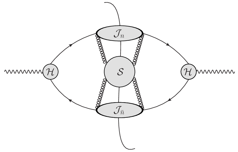
The soft subprocess $\tilde{S}\left({N_{0}}/{N}{Q}/{\mu},\alpha_{s}(\mu)\right)$ describes the interaction between the two jets of hard collinear particles through soft gluon exchange. It can be therefore defined in a gauge invariant way as a correlator of Wilson lines

$\displaystyle\tilde{S}\left(\frac{N_{0}}{N}\frac{Q}{\mu},\alpha_{s}(\mu)\right)=\frac{Q}{N_{c}}\int d\tau_{s}{\rm e}^{-\tau_{s}N}\sum_{k_{eik}}\langle 0|W^{\dagger}_{\bar{n}}(0)W^{\dagger}_{n}(0)|k_{eik}\rangle\mathcal{J}_{cut}(\tau_{s}Q)\langle k_{eik}|W_{n}(0)W_{\bar{n}}(0)|0\rangle,$

(13)

where we defined $\tau_{s}=w/Q$. $W_{n}$ and $W_{\bar{n}}$ are Wilson lines

$\displaystyle W_{n}(y)={\rm\textbf{P}}{\rm exp}\left(ig\int_{0}^{\infty}ds\,n\cdot A(ns+y)\right),$

(14)

describing the eikonal interaction of soft gluons with the fast moving quarks along the light-like directions $n^{\mu}$ and $\bar{n}^{\mu}$ respectively. $A(ns+y)$ in eq. (14) denotes the gluon field in QCD. The sum runs over the final states $|k_{eik}\rangle$ involving $k$ soft particles whose phase space is constrained according to the thrust trigger function $\mathcal{J}_{cut}(\tau Q^{2})$. Both soft and soft-collinear contributions are encoded into the soft subprocess. The two-loop expression was computed analytically in [29] by performing direct phase-space cuts. The results are in agreement with those presented in [32, 33]. The collinear subprocess $\mathcal{J}$ ($\mathcal{\bar{J}}$) describes the decay of the jet-initiating hard quark (antiquark) into a jet of collinear particles moving along the $n^{\mu}$ ($\bar{n}^{\mu}$) direction. It is therefore an inclusive quantity which can be found in many other relevant QCD processes such as deep inelastic scattering and heavy quarks decay [22, 37, 30]. The short-distance hard function $H\left({Q}/{\mu},\alpha_{s}(\mu)\right)=|\mathcal{H}\left({Q}/{\mu},\alpha_{s}(\mu)\right)|^{2}$ takes into account the hard virtual corrections to the quark-antiquark production subprocess. It is free of large logarithms and it can be generally defined such that Eq. (10) reproduces the fixed-order cross section up to power suppressed terms.
Using the Renormalisation Group evolution of the soft and collinear subprocesses [37, 30, 29], we can recast eq. (12) as

	$\displaystyle R_{T}(\tau)=$	$\displaystyle H\left(\frac{Q}{\mu},\alpha_{s}(\mu)\right)\frac{1}{2\pi i}\int_{C}\frac{dN}{N}\,{\rm e}^{\tau N}\tilde{J}^{2}\left(1,\alpha_{s}(\sqrt{\frac{N_{0}}{N}}Q)\right)\tilde{S}\left(1,\alpha_{s}(\frac{N_{0}Q}{N})\right)\times$
		$\displaystyle{\rm exp}\bigg\{-2\int_{\frac{N_{0}}{N}}^{1}\frac{du}{u}\left[\int_{u^{2}Q^{2}}^{uQ^{2}}\frac{dk^{2}}{k^{2}}\mathcal{A}(\alpha_{s}(k^{2}))+\mathcal{B}(\alpha_{s}(uQ^{2}))\right]\bigg\},$		(15)

where the two coefficients $\mathcal{A}(\alpha_{s})$ and $\mathcal{B}(\alpha_{s})$ can be computed in perturbation theory. The coefficient $\mathcal{A}(\alpha_{s})$ reads

$\displaystyle\mathcal{A}(\alpha_{s})$

$\displaystyle=\Gamma_{\rm{cusp}}(\alpha_{s})-\beta(\alpha_{s})\frac{\partial\Gamma_{\rm{soft}}(\alpha_{s})}{\partial\alpha_{s}},$

where $\Gamma_{\rm{cusp}}(\alpha_{s})$ and $\Gamma_{\rm{soft}}(\alpha_{s})$ are the cusp and the soft anomalous dimensions respectively. The former, together with the coefficient $\mathcal{B}(\alpha_{s})$ can be extracted from the asymptotic limit of the $P_{qq}(\alpha_{s},z)$ splitting function [38, 31] as $z\rightarrow 1$

$\displaystyle P_{qq}(\alpha_{s},z)\rightarrow 2\frac{\Gamma_{\rm{cusp}}(\alpha_{s})}{(1-z)_{+}}+2\mathcal{B}(\alpha_{s})\delta(1-z)+...$

(17)

The integration countour in eq. (15) runs parallel to the imaginary axis on the right of all singularities of the integrand. From eq. (15) we see that the $u$-integral in the exponent is regularised by the lower bound $\frac{N_{0}}{N}$. Such a bound acts as an infrared regulator which prevents the strong coupling constant from being evaluated at non-perturbative scales ($\leq\Lambda_{QCD}$). Then, the contour in eq. (15) should be set away from all the singularities (in particular from the Landau pole). Nevertheless, for resummation purposes we can set the contour on the left of the Landau singularity since it would contribute with a non-logarithmic effect suppressed with some negative power of the center-of-mass energy scale. The inversion of the Laplace transform can be performed analytically by using the residue theorem as shown in [11, 29] and results in

$\displaystyle R_{T}(\tau)=\bigg(1+\sum_{k=1}^{\infty}C_{k}\bigg(\frac{\alpha_{s}}{2\pi}\bigg)^{k}\bigg){\rm exp}\left[\log\frac{1}{\tau}g_{1}(\lambda)+g_{2}(\lambda)+\frac{\alpha_{s}}{\pi}\beta_{0}g_{3}(\lambda)+\left(\frac{\alpha_{s}}{2\pi}\right)^{3}G_{31}\log\frac{1}{\tau}\right],$

(18)

where

	$\displaystyle g_{1}(\lambda)=$	$\displaystyle\,\,\,f_{1}(\lambda),$
	$\displaystyle g_{2}(\lambda)=$	$\displaystyle\,\,\,f_{2}(\lambda)-\log\Gamma(1-f_{1}(\lambda)-\lambda f_{1}^{\prime}(\lambda)),$
	$\displaystyle g_{3}(\lambda)=$	$\displaystyle\,\,\,f_{3}(\lambda)+\left(f_{1}^{\prime}(\lambda)+\frac{1}{2}\lambda f_{1}^{\prime\prime}(\lambda)\right)\left(\psi^{(0)}(1-\gamma(\lambda))^{2}-\psi^{(1)}(1-\gamma(\lambda))\right)$
		$\displaystyle+f_{2}^{\prime}(\lambda)\psi^{(0)}(1-\gamma(\lambda))+C_{F}/\beta_{0}\left(\gamma_{E}\left(3/2-\gamma_{E}\right)-\pi^{2}/6\right).$		(19)

The functions $f_{i}(\lambda)$ as well as the constants $C_{1}$, $C_{2}$ and $G_{31}$ are defined in [29], while the $C_{3}$ constant term is still analytically unknown. We fit the latter numerically using the fixed order Monte Carlo parton-level generator EERAD3. The fit is performed by subtracting the $\mathcal{O}(\alpha_{s}^{3})$ logarithmic structure from the fixed-order result and taking (numerically) the asymptotic limit $\tau\rightarrow 0$.
EERAD3 is run with a technical cutoff $y_{0}=10^{-5}$ which affects the thrust distribution below $\tau_{0}\sim\sqrt{y_{0}}$. This forbids us from probing the far infrared region and we perform the fit for values of $\tau$ larger than $\tau_{0}$. Numerical fixed order results are obtained with $6\times 10^{7}$ points for the leading colour contribution and $10^{7}$ points for the subleading colour structures. Because of the presence of large fluctuations in the Monte Carlo results, each color contribution is fitted separately over an interval where the distribution is stable and the different results are combined to find the numerical value of $C_{3}$. As an alternative approach we first sum up all the color contributions and then fit $C_{3}$. We consider the difference between the two approaches as a systematic error and as final result we obtain

$$C_{3}=-1050\pm 180(\textrm{stat.})\pm 500(\textrm{syst.})\,.$$

(20)

In this section we match the obtained resummed distribution (18) to the NNLO fixed order prediction. The matching formalism must avoid double counting and allow to access theoretical uncertainties. We compare the $R$-matching and ${\rm log}(R)$-matching scheme described in [14].

In Figure 3 we compare the differential cross section of the new matched NNLL+NNLO results with the old NLL+NNLO derived in [42]. The modification due to the resummation is sizable, leading to a $8\%$ increase of the distribution around the peak region. The effect of the additional resummed subleading logarithms becomes progressively less important towards the multijet region, where the increase is nevertheless of about $5\%$. It is interesting to note that the matching of NNLO with NNLL resummation shifts the pure NNLO result also in the multijet region (Figure 5). This was not the case for NLL+NNLO, for which the impact of resummation in the region of large $\tau$ was negligible. This is another sign of the importance of the NNLL contribution.

The renormalisation scale dependence, which was observed to increase from pure NNLO to NLL+NNLO [42, 45] because of a mismatch in the cancellation of renormalisation scale logarithms, is obtained by varying $0.5<x_{\mu}<2$. It decreases at NNLL+NNLO by 20% in the peak region compared to NLL+NNLO. The magnitude of the scale uncertainty varies between 4% in the 3-jet region and 5% around the peak. In Figure 5 we compare the $R$-matching and the $\log(R)$-matching scheme predictions at NNLL+NNLO. The difference between the two matching prescriptions is tiny and lies well below the scale uncertainty. This implies a very good stability of the theoretical predictions under variation of the matching scheme.

One further source of arbitrariness is the choice of the logarithms to be resummed. In fact, it is not clear whether powers of $\alpha_{s}\log(1/\tau)$ or powers of e.g. $\alpha_{s}\log(2/\tau)$ have to be resummed. The origin of this arbitrariness has to do with how much of the non-logarithmic part of the fixed-order prediction is exponentiated together with the logarithms. We can express this arbitrariness by introducing a new parameter $x_{L}$, which rescales the logarithms as  [14]: $L\,\rightarrow\,\hat{L}=\log\left(1/(x_{L}\tau)\right)$.

We can estimate the related uncertainty by varying the parameter $x_{L}$. In Ref. [14] several prescriptions are given on how to set the correct variation range for $x_{L}$ for different observables. For the sake of simplicity and since we are not performing a fit of the strong coupling constant, we choose to vary $x_{L}$ within the canonical interval $0.5<x_{L}<2$, similarly to what is chosen to quantify the renormalisation scale uncertainty. This choice is also close to the nominal range of variation proposed in [14]. The impact of this variation is shown in Figure 6. The left plots show a comparison of the $x_{L}$-dependence between NLL+NNLO and NNLL+NNLO predictions. The lower plot allows to quantify the reduction of the uncertainty due to a variation $x_{L}$. Apart from the far infrared region, it is observed to decrease by $50\%$ in the peak region. The scale-dependence reduction is smaller towards the multijet region, where the contribution of the logarithmic part becomes less important. The resummation uncertainty at NNLL+NNLO varies between $2\%$ and $3\%$. In the right plot the same comparison is made at NNLL+NNLO using the $R$-matching and $\log(R)$-matching schemes. We observe a similar $x_{L}$-dependence in both schemes.