Super-aging correlation function and ergodicity breaking for Brownian Motion in logarithmic potentials

Ergodicity is a central concept in the theory of stochastic processes. A random variable $A$ is said to be ergodic when its time average $\bar{A}(t)=(1/t)\int_{0}^{t}dt^{\prime}A(t^{\prime})$ over a single realization in the limit of infinitely long times is equal to the equilibrium ensemble average $\langle A\rangle=\int dA\,AP(A)$ over many realizations of the process [1]. Here $P(A)$ is the equilibrium probability density for the random variable $A$. For ergodic variables, the width of the probability distribution of the random time average vanishes in the long-time limit, and the distribution reduces asymptotically to a delta function centered on the ensemble average, $Q\left(\bar{A},t\right)\rightarrow\delta\left(\bar{A}-\langle A\rangle\right)$. For nonergodic variables, the time average remains a stochastic quantity even in the infinite time limit. A general criterion for the ergodicity of a process is given by the Khinchin theorem [2], which asserts that a stationary process is ergodic if its autocorrelation function $\langle A(t)A(t_{0})\rangle\rightarrow\langle A\rangle^{2}$ when $|t-t_{0}|\rightarrow\infty$. However, for processes for which a stationary autocorrelation function does not exist, we cannot use the Khinchin theorem to predict the ergodic properties of the process. For specific systems, there are generalizations of the Khinchin theorem to the nonstationary case [3, 4], but for a general system, the ergodic properties are not straightforward to predict. Meanwhile, for finite times, the time average will be a random variable for any process, ergodic or not. Since in all experiments the measurement time might be large, but is always finite, it is essential to determine the properties of the distribution of the time average, as the latter cannot be evaluated using the equilibrium measure $P(A)$. The distribution of the time average has been investigated for continuous-time random-walk models [5], but no general theory exists. In Ref. [6], we have provided a general expression for the variance of the time-averaged position $\bar{x}(t)$ for an overdamped Brownian particle in a binding field and showed that, in the special case of a logarithmic potential, the ergodic hypothesis breaks down.

In the present paper, we study in more detail the variance $\bar{\sigma}^{2}(t)=\langle\bar{x}^{2}(t)\rangle-\langle\bar{x}(t)\rangle^{2}$ of the time-averaged position of an overdamped Brownian particle moving in a confining potential that is asymptotically logarithmic. This system defines an important class of processes which has found widespread applications in the description of the dynamics of particles near a long, charged polymer [7], momentum diffusion in dissipative optical lattices [8, 9, 10, 11, 12, 13, 14, 15], probe particles in one-dimensional driven fluids [16], self-gravitating Brownian particles [17], long-range interacting systems [18, 19, 20], and diffusion of fractals [21], as well as the dynamics of bubbles in DNA molecules [22, 23, 24, 25], of vortices [26], and of trapped nanoparticles [27]. A striking characteristic of these systems is that the equilibrium probability distribution possesses a power-law tail which may lead to diverging moments and ergodicity breaking [28]. Their anomalous behavior is controlled by a single parameter that is related to the depth of the potential. In the following, we derive explicit long-time expressions for the two-time correlation function and for the time-averaged variance of the position of the particle, and we investigate in detail the diffusive and ergodic properties of the system for large, but finite times. We show how a super-aging correlation function describes this system, even when the stationary Boltzmann distribution is normalizable.

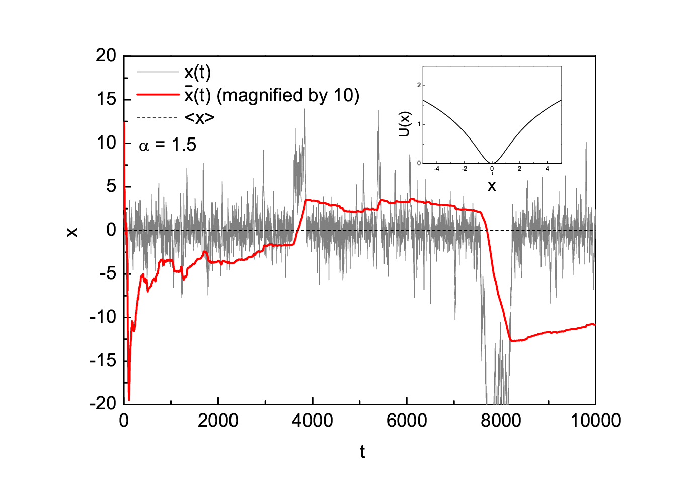
Figure 1 shows a typical trajectory of a Brownian particle in a logarithmic potential in the nonergodic phase, obeying the overdamped Langevin equation

$\displaystyle\frac{dx}{dt}=-\frac{1}{m\gamma}\frac{\partial U(x)}{\partial x}+F(t)$

(1)

with $U(x)=(U_{0}/2)\ln(1+x^{2})$ and the fluctuating Gaussian noise $F(t)$, $\langle F(t)F(t^{\prime})\rangle=(2k_{B}T/(m\gamma))\delta(t-t^{\prime})$. Here, $m$ is the mass of the particle, $\gamma$ is the friction coefficient, $k_{B}$ is the Boltzmann constant and $T$ is the temperature. Obviously the time average $\bar{x}(t)=(1/t)\int_{0}^{t}dt^{\prime}x(t^{\prime})$ does not converge to the ensemble average $\langle x\rangle=0$ even for long times. The reason for this behavior is the long excursions of the particle into the tails of the potential, where the slope and thus the restoring force tends to zero for $x\gg 1$. On average, these excursions get ever longer as time increases and thus dominate the time average for all times. Our goal is to characterize the nonergodic behavior of this process.

The outline of the paper is as follows. In Section II, we solve the Fokker-Planck equation corresponding to Eq. (1) for the Brownian particle by transforming it into a Schrödinger-like equation and using an eigenfunction expansion. In Section III, we explicitly construct the conditional probability density from the eigenfunction expansion and determine its asymptotic long-time behavior, as well as those of the first and second moments of the position variable. We then use the conditional probability density in Section IV to compute the two-time position correlation function, which exhibits either stationary behavior or nonstationary, super-aging behavior, depending on the depth of the potential. Finally, in Section V, we evaluate the variance of the time-averaged position and show the existence of a threshold for the potential depth below which ergodicity is broken. Parts of our results were obtained in Ref. [6] with the help of a scaling ansatz. We provide here a complementary and more detailed derivation.

We consider an overdamped Brownian particle moving in a symmetric ($U(x)=U(-x)$) potential $U(x)$ that is asymptotically logarithmic for large $|x|\gg a$, $U(x)\simeq U_{0}\ln(|x|/a)$; during the calculation, we will set $a=1$. For $a\neq 1$, the variable $x$ in our results should be replaced by $x/a$. An example for such a potential is $U(x)=(U_{0}/2)\ln(1+x^{2})$, which is what we use for our numerical Langevin simulations. The dynamics of the particle is governed by the Fokker-Planck equation for the probability density $W(x,t)$ corresponding to the Langevin equation (1),

$\displaystyle\frac{\partial}{\partial t}W(x,t)$

$\displaystyle=\frac{D}{k_{B}T}\frac{\partial}{\partial x}\left(U^{\prime}(x)W(x,t)\right)+D\frac{\partial^{2}}{\partial x^{2}}W(x,t)\ ,$

(2)

where $D=k_{B}T/(m\gamma)$ is the diffusion coefficient. In the following, we set the mass of the particle to $m=1$. The stationary equilibrium solution to Eq. (2) is given by $W_{\text{eq}}(x)=\exp(-U(x)/(k_{B}T))/Z$ with the normalizing partition function $Z=\int dx\exp(-U(x)/(k_{B}T))$. As we will see, the partition function $Z$ and thus the stationary probability density do not always exist for the logarithmic potential. Since for the logarithmic potential, we have asymptotically $U^{\prime}(x)\simeq U_{0}/|x|$, both the first (drift) and second (diffusion) term on the right-hand side of Eq. (2) scale as $1/x^{2}$ [29]. This scaling is responsible for the interesting effects discussed in the following. The addition of a linear force to the logarithmic potential breaks this scaling and leads to a very different behavior [30, 31, 32, 33].

Our goal is to evaluate the long-time behavior of the variance of the time-averaged position, $\bar{x}(t)=\int_{0}^{t}dt^{\prime}\,x(t^{\prime})/t$, which is given by,

	$\displaystyle\bar{\sigma}^{2}(t)$	$\displaystyle=\langle\bar{x}^{2}(t)\rangle-\langle\bar{x}(t)\rangle^{2}$
		$\displaystyle=\frac{1}{t^{2}}\left[\int_{0}^{t}dt^{\prime\prime}\int_{0}^{t}dt^{\prime}\,C(t^{\prime\prime},t^{\prime})\right.$
		$\displaystyle\quad\left.-\left(\int_{0}^{t}dt^{\prime}\langle x(t^{\prime})\rangle\right)^{2}\right]\ .$		(3)

For an ergodic system, we expect $\bar{x}(t)\rightarrow\langle x\rangle_{\text{eq}}=0$ and thus $\bar{\sigma}^{2}(t)\rightarrow 0$. The two-time position correlation function $C(t,t_{0})=\langle x(t)x(t_{0})\rangle$ in Eq. (3) can be expressed in the form [34],

$\displaystyle C(t,t_{0})$

$\displaystyle=\int_{-\infty}^{\infty}dx\int_{-\infty}^{\infty}dx_{0}\,xx_{0}P(x,t|x_{0},t_{0})W(x_{0},t_{0})\ ,$

(4)

where $P(x,t|x_{0},t_{0})$ is the conditional probability density. This expression is correct for a prior initial condition of a narrow diffusing packet (e.g. a Gaussian distribution centered on the origin) and sufficiently long times $t_{0}$. For power-law initial conditions, a different behavior is expected; see Refs. [35, 36]. For most potentials $U(x)$ (e.g. harmonic), $W(x,t_{0})$ in Eq. (4) can be replaced by the stationary probability density $W_{\text{eq}}(x)$. For the logarithmic potential, however, it turns out that the integrals in Eq. (4) do not always converge and we need to use the explicitly time-dependent probability density $W(x,t_{0})$. In order to solve the Fokker-Planck equation (2), we transform it into a Schrödinger equation and employ an eigenfunction expansion. Writing the probability density as $W(x,t)=\chi(x)\psi(x,t)$ with the function $\chi(x)=\exp{(-U(x)/(2k_{B}T))}$, we obtain the following equation for $\psi(x,t)$ [34],

	$\displaystyle-\frac{1}{D}\frac{\partial}{\partial t}\psi(x,t)=$	$\displaystyle-\frac{\partial^{2}}{\partial x^{2}}\psi(x,t)$
	$\displaystyle+\left(\frac{1}{4k_{B}^{2}T^{2}}\right.$	$\displaystyle U^{\prime 2}(x)+\left.\frac{1}{2k_{B}T}U^{\prime\prime}(x)\right)\psi(x,t)\ .$		(5)

Equation (5) has the form of an imaginary-time Schrödinger equation with the effective potential,

$\displaystyle U_{\text{eff}}(x)=\frac{1}{4k_{B}^{2}T^{2}}U^{\prime 2}(x)+\frac{1}{2k_{B}T}U^{\prime\prime}(x)\ .$

(6)

Its general solution is given by the expansion,

$\displaystyle\psi(x,t)=\sum_{\lambda}\eta_{\lambda}\psi_{\lambda}(x)\,e^{-D\lambda t}\ ,$

(7)

where $\psi_{\lambda}(x)$ are the eigenfunctions of Eq. (5),

$\displaystyle\left[-\frac{\partial^{2}}{\partial x^{2}}+U_{\text{eff}}(x)\right]\psi_{\lambda}(x)=\lambda\psi_{\lambda}(x)\ .$

(8)

Since the Hamiltonian is symmetric in $x$, we look for solutions of the eigenvalue equation (8) that have either even or odd parity [37]. To simplify the calculations, we use the potential

$\displaystyle U(x)=U_{0}\ln(|x|)\Theta(|x|-1)\ ,$

(9)

which has the desired asymptotic form $U(x)\simeq U_{0}\ln|x|$, $|x|>1$, and is zero for $|x|<1$. The asymptotic long-time behavior of the system is up to a constant factor independent of the potential near the origin and our calculation can be generalized to arbitrary, asymptotically logarithmic potentials [38]. For $|x|>1$, the eigenfunctions are given by [9],

	$\displaystyle\psi_{k,e}(x)$	$\displaystyle=A_{k}\sqrt{|x|}\left(a_{1k}J_{\alpha}(|kx|)+a_{2k}J_{-\alpha}(|kx|)\right),$
	$\displaystyle\psi_{0}(x)$	$\displaystyle=A\left(a_{1}|x|^{\frac{1}{2}-\alpha}+a_{2}|x|^{\alpha+\frac{1}{2}}\right),$		(10)
	$\displaystyle\psi_{k,o}(x)$	$\displaystyle=B_{k}\,\text{sgn}(kx)\sqrt{|x|}\left(b_{1k}J_{\alpha}(|kx|)+b_{2k}J_{-\alpha}(|kx|)\right),$

with $k=\pm\sqrt{\lambda}$ and

$\displaystyle\alpha=\frac{U_{0}}{2k_{B}T}+\frac{1}{2}\ .$

(11)

The subscript $e$ ($o$) refers to the even (odd) solutions, $J_{\alpha}(x)$ denotes the Bessel function of the first kind, $A$, $A_{k}$ and $B_{k}$ are normalization constants and $a_{i}$, $a_{ik}$ and $b_{ik}$ ($i,j\in\{1,2\}$) will be determined by the boundary conditions at $x=\pm 1$. The spectrum for $\alpha>1$ consists of a single discrete ground state for $k=0$, $\psi_{0}(x)$, which is an even function of $x$, and a continuum of excited states for $k>0$. For $\alpha<1$, the discrete solution $\psi_{0}(x)$ is non-normalizable (see below) and the spectrum is thus pure continuous. The parameter $\alpha>1/2$, which measures the ratio of the potential depth $U_{0}$ and the temperature $T$, will turn out to be the key quantity controlling the long-time behavior of the particle. The structure of the spectrum with the continuum of excited states starting at $k=0$ and thus no gap to the bound state [39] is responsible for the anomalous behavior and sensitive dependence on $\alpha$. Using the eigenstates (10), the solution of the Fokker-Planck equation (2) is

	$\displaystyle W(x,t)$	$\displaystyle=\mathfrak{a}_{0}\chi(x)\psi_{0}(x)$
		$\displaystyle+\chi(x)\int_{-\infty}^{\infty}dk\,\mathfrak{a}_{k}\psi_{k,e}(x)\,e^{-Dk^{2}t}$
		$\displaystyle+\chi(x)\int_{-\infty}^{\infty}dk\,\mathfrak{b}_{k}\psi_{k,o}(x)\,e^{-Dk^{2}t}\ .$		(12)

For convenience, we sum over $\pm k$ with $a_{ik}=a_{i(-k)}$ and $b_{ik}=b_{i(-k)}$. The coefficients $\mathfrak{a}_{k}$ and $\mathfrak{b}_{k}$ are determined by the initial condition. For $|x|<1$, the potential vanishes and thus the corresponding eigenfunctions are

	$\displaystyle\tilde{\psi}_{k,e}(x)$	$\displaystyle=A_{k}\cos(kx)\ ,$
	$\displaystyle\tilde{\psi}_{0}(x)$	$\displaystyle=A\ ,$
	$\displaystyle\tilde{\psi}_{k,o}(x)$	$\displaystyle=B_{k}\sin(kx)\ ,$		(13)

with the boundary conditions at $x=1$,

	$\displaystyle\psi_{k,e}(1)$	$\displaystyle=\tilde{\psi}_{k,e}(1)\ ,$
	$\displaystyle\psi_{k,e}^{\prime}(1)$	$\displaystyle=\tilde{\psi}_{k,e}^{\prime}(1)-\frac{U_{0}}{2k_{B}T}\psi_{k,e}(1)\ .$		(14)

The last term on the right-hand side stems from the discontinuity of $U^{\prime}(x)$ at $x=1$ (similar boundary conditions are obtained for the ground state and the odd eigenfunctions). From this, the coefficients for the ground state are easily seen to be $a_{1}=1$ and $a_{2}=0$.

The two integrals in the solution (12) can be regarded as Laplace transforms. The large $t$ behavior of the system is then determined by the small $k$ expansion of the eigenfunctions, according to the final value theorem [40]. Using the Taylor expansion of the Bessel function [41], (Eq. (9.1.7)),

$\displaystyle J_{\alpha}(k)$

$\displaystyle\simeq\frac{1}{\Gamma(\alpha+1)}\left(\frac{k}{2}\right)^{\alpha}\ ,$

(15)

and those of the sine and cosine, we find from Eqs. (10), (13) and (14) the coefficients of the excited states to leading order in $k$,

	$\displaystyle a_{1k}$	$\displaystyle\simeq-\Gamma(\alpha)\frac{2\alpha-1}{\alpha-1}\left(\frac{k}{2}\right)^{2-\alpha}\ ,$
	$\displaystyle a_{2k}$	$\displaystyle\simeq\Gamma(1-\alpha)\left(\frac{k}{2}\right)^{\alpha}\ ,$
	$\displaystyle b_{1k}$	$\displaystyle\simeq\Gamma(\alpha)\left(\frac{k}{2}\right)^{1-\alpha}\ ,$
	$\displaystyle b_{2k}$	$\displaystyle\simeq\Gamma(1-\alpha)\frac{2\alpha-1}{\alpha}\left(\frac{k}{2}\right)^{\alpha+1}\ .$		(16)

The probability density $W(x,t)$ should be properly normalized at all times. For the discrete ground state, the normalization integral reads,

$\displaystyle 2\int_{0}^{1}dx\,\tilde{\psi}_{0}^{2}(x)+2\int_{1}^{\infty}dx\,{\psi}_{0}^{2}(x)=1\ .$

(17)

As it turns out, the ground state is only normalizable for $\alpha>1$. The corresponding normalization constant is,

$\displaystyle A^{2}=\frac{\alpha-1}{2\alpha-1}=\frac{1}{Z}\ .$

(18)

Thus the discrete solution is $\psi_{0}(x)=(1/\sqrt{Z})\,|x|^{-\alpha+1/2}$, which is precisely the square root of the normalized stationary solution of the Fokker-Planck equation (2) for $|x|>1$. For $\alpha<1$, there is no normalizable ground state and thus no stationary probability density. Since the excited states form a continuum, they need to be normalized to a delta function,

	$\displaystyle 2$	$\displaystyle\int_{0}^{1}dx\,\tilde{\psi}_{k,e/o}(x)\tilde{\psi}_{k^{\prime},e/o}(x)$
		$\displaystyle+2\int_{1}^{\infty}dx\,{\psi}_{k,e/o}(x){\psi}_{k^{\prime},e/o}(x)=\delta(k-k^{\prime})\ .$		(19)

Realizing that the main contribution to the normalization integral (19) comes from large values of $x$, we use the asymptotic expansion of the Bessel function [41], (Eq. (9.2.1)),

$\displaystyle J_{\alpha}(kx)\simeq\sqrt{\frac{2}{\pi kx}}\cos\left(kx-\frac{\pi\alpha}{2}-\frac{\pi}{4}\right)\ ,$

(20)

to obtain the expressions,

	$\displaystyle A_{k}^{2}\simeq\frac{k}{4}\frac{1}{a_{1k}^{2}+a_{2k}^{2}+2a_{1k}a_{2k}\cos\left(2\phi_{\alpha}-\frac{\pi}{2}\right)}\ ,$
	$\displaystyle B_{k}^{2}\simeq\frac{k}{4}\frac{1}{b_{1k}^{2}+b_{2k}^{2}+2b_{1k}b_{2k}\cos\left(2\phi_{\alpha}-\frac{\pi}{2}\right)}\ ,$		(21)

where $\phi_{\alpha}=\alpha\pi/2+\pi/4$. Since the coefficients $a_{ik}$ and $b_{jk}$ are only known up to leading order in $k$, we further need to expand the normalization constants $A_{k}$ and $B_{k}$ to leading order in $k$ in order to be consistent. Since $\alpha>1/2$, $b_{1k}$ will always dominate $b_{2k}$ and we have

$\displaystyle B_{k}^{2}\simeq\frac{k}{4}\frac{1}{b_{1k}^{2}}\ .$

(22)

However, the relative magnitude of $a_{1k}$ and $a_{2k}$ depends on the value of $\alpha$. For $\alpha>1$, $a_{1k}$ dominates $a_{2k}$, and vice versa for $\alpha<1$. This leads to

$\displaystyle A_{k}^{2}\simeq\left\{\begin{array}[]{ll}\frac{k}{4}\frac{1}{a_{1k}^{2}}&\text{for}\quad\alpha>1\\[8.61108pt] \frac{k}{4}\frac{1}{a_{2k}^{2}}&\text{for}\quad\alpha<1\ .\end{array}\right.$

The final pieces of information needed to fully determine the solution (12) are the expansion coefficients $\mathfrak{a}_{k}$ and $\mathfrak{b}_{k}$. They are related to the initial condition $W(x,0)$ by,

	$\displaystyle\mathfrak{a}_{k}$	$\displaystyle=\int_{-\infty}^{\infty}dx\,\psi_{k,e}(x)\frac{W(x,0)}{\chi(x)}\ ,$
	$\displaystyle\mathfrak{a}_{0}$	$\displaystyle=\int_{-\infty}^{\infty}dx\,\psi_{0}(x)\frac{W(x,0)}{\chi(x)}\ ,$
	$\displaystyle\mathfrak{b}_{k}$	$\displaystyle=\int_{-\infty}^{\infty}dx\,\psi_{k,o}(x)\frac{W(x,0)}{\chi(x)}\ .$		(25)

The evaluation of the correlation function (4) requires the computation of the conditional probability density $P(x,t|x_{0},t_{0})$, the solution of the Fokker-Planck equation (2) with the initial condition $P(x,t_{0})=\delta(x-x_{0})$ [34]. Accordingly, it is of the form (12) with the time variable $t$ replaced by the time difference

$\displaystyle\tau=t-t_{0}\ .$

(26)

The expansion coefficients are then, from Eq. (25),

	$\displaystyle\mathfrak{a}_{k}$	$\displaystyle=\frac{\psi_{k,e}(x_{0})}{\chi(x_{0})}\ ,$
	$\displaystyle\mathfrak{a}_{0}$	$\displaystyle=\frac{\psi_{0}(x_{0})}{\chi(x_{0})}=A\ ,$
	$\displaystyle\mathfrak{b}_{k}$	$\displaystyle=\frac{\psi_{k,o}(x_{0})}{\chi(x_{0})}\ .$		(27)

As a result, we have for $x>1$ and $x_{0}>1$ (the behavior for negative $x$ and $x_{0}$ follows from symmetry),

		$\displaystyle P(x,t|x_{0},t_{0})=A\chi(x)\psi_{0}(x)$
		$\displaystyle\quad+2\frac{\chi(x)}{\chi(x_{0})}\int_{0}^{\infty}dk\,\psi_{k,e}(x_{0})\psi_{k,e}(x)e^{-Dk^{2}\tau}$
		$\displaystyle\quad+2\frac{\chi(x)}{\chi(x_{0})}\int_{0}^{\infty}dk\,\psi_{k,o}(x_{0})\psi_{k,o}(x)e^{-Dk^{2}\tau}$
		$\displaystyle\simeq A^{2}x^{1-2\alpha}+2\,x^{1-\alpha}x_{0}^{\alpha}\int_{0}^{\infty}dk$
		$\displaystyle\quad\times\Big[A_{k}^{2}\left(a_{1k}J_{\alpha}(kx_{0})+a_{2k}J_{-\alpha}(kx_{0})\right)$
		$\displaystyle\qquad\times\left(a_{1k}J_{\alpha}(kx)+a_{2k}J_{-\alpha}(kx)\right)e^{-Dk^{2}\tau}$
		$\displaystyle\qquad+B_{k}^{2}\left(b_{1k}J_{\alpha}(kx_{0})+b_{2k}J_{-\alpha}(kx_{0})\right)$
		$\displaystyle\qquad\times\left(b_{1k}J_{\alpha}(kx)+b_{2k}J_{-\alpha}(kx)\right)e^{-Dk^{2}\tau}\Big]\ .$		(28)

For completeness, the discussion of the cases where either $x$ or $x_{0}$ is smaller than $1$ is given in Appendix A. The very first term on the right-hand side of Eq. (28) is the contribution of the stationary state and only appears for $\alpha>1$ (since $A=0$ for $\alpha<1$). The expansion of the product in the integral yields four terms for the even contributions (those containing the $a_{ik}$-coefficients) and four terms for the odd contributions (those containing the $b_{jk}$-coefficients). Since the leading order of the normalization constant $A_{k}$ is different depending on whether $\alpha$ is larger or smaller than $1$ (see Eq. (II)), we have to examine 12 integrals in total (some of which are fortunately the same). However, all these integrals share the same basic structure:

	$\displaystyle\mathfrak{I}_{e/o,\mu,\nu}(z,y)$	$\displaystyle=c_{e/o,\mu,\nu}(z,y)$
		$\displaystyle\,\times\int_{0}^{\infty}du\,u^{\lambda_{e/o,\mu,\nu}}J_{\mu}(2uy)J_{\nu}(2uz)e^{-u^{2}}\ ,$		(29)

where $\mu$ and $\nu$ are equal to $\pm\alpha$ and both the $u$-independent factor $c_{e/o,\mu,\nu}(z,y)$ and the exponent $\lambda_{e/o,\mu,\nu}$ are different depending on the combination of $\mu$ and $\nu$. Here we have introduced the variables $u=k(D\tau)^{1/2}$, $z=x/(4D\tau)^{1/2}$ and $y=x_{0}/(4D\tau)^{1/2}$. We can then write Eq. (28) as,

	$\displaystyle P(x$	$\displaystyle,t|x_{0},t_{0})\simeq A^{2}x^{-2\alpha+1}$
		$\displaystyle\,+\sum_{e,o}\sum_{\mu,\nu=\pm\alpha}\,\left(\sqrt{D\tau}\right)^{2-\lambda_{e/o,\mu,\nu}}\mathfrak{I}_{e/o,\mu,\nu}(z,y)\ .$		(30)

It is important to note that the main contribution to the integrals $\mathfrak{I}_{e/o,\mu,\nu}(z,y)$ comes from small values of $u$ as the exponential factor causes the integrand to vanish exponentially for large values of $u$ and all other functions increase at most as a power of $u$. Table 1 gives a summary of all the values of $\mu$, $\nu$, and $\lambda_{e/o,\mu,\nu}$, as well as the prefactors $c_{e/o,\mu,\nu}(z,y)$ of the respective integrals.

References

• [1] A. Papoulis, Probability, Random Variables, and Stochastic Processes (McGraw-Hill, New York, 1991).
• [2] A.I. Khinchin, Mathematical Foundations of Statistical Mechanics (Dover, New York, 1949).
• [3] S. Burov, R. Metzler and E. Barkai, Proc. Natl. Acad. Sci. (U.S.A.) 107, 13228 (2010).
• [4] A. Weron and M. Magdziarz, Phys. Rev. Lett. 105, 260603 (2010).
• [5] A. Rebenshtok and E. Barkai, Phys. Rev. Lett. 99, 210601 (2007).
• [6] A. Dechant, E. Lutz, D.A. Kessler and E. Barkai, Phys. Rev. Lett. 107, 240603 (2011a).
• [7] G.S. Manning, J. Chem. Phys. 51, 924 (1969).
• [8] Y. Castin, J. Dalibard and C. Cohen-Tannoudji, Proceedings of the LIKE workshop pp. 5–24 (1990).
• [9] S. Marksteiner, K. Ellinger and P. Zoller, Phys. Rev. A 53, 3409 (1996).
• [10] H. Katori, S. Schlipf and H. Walther, Phys. Rev. Lett. 79, 2221 (1997).
• [11] E. Lutz, Phys. Rev. A 67, 051402(R) (2003).
• [12] P. Douglas, S. Bergamini and F. Renzoni, Phys. Rev. Lett 96, 110601 (2006).
• [13] Y. Sagi, M. Brook, I. Almog and N. Davidson, Phys. Rev. Lett. 108, 093002 (2012).
• [14] D. A. Kessler and E. Barkai, Phys. Rev. Lett. (accepted, 2012).
• [15] A. Dechant and E. Lutz, Phys. Rev. Lett. (accepted, 2012).
• [16] E. Levine, D. Mukamel and G.M. Schütz, Europhys. Lett. 70, 565 (2005).
• [17] P.H. Chavanis and R. Manella, Eur. Phys. J. B 78, 139 (2010).
• [18] F. Bouchet and T. Dauxois, Phys. Rev. E 72, 045103(R) (2005a).
• [19] F. Bouchet and T. Dauxois, J. Phys. Conf. Ser. 7, 34 (2005b).
• [20] P.H. Chavanis and M. Lemou, Eur. Phys. J. B 59, 217 (2007).
• [21] M. O. Vlad, Chaos, Solitons Fractals 4, 191 (1994).
• [22] H.C. Fogedby and R. Metzler, Phys. Rev. E 76, 061915 (2007a).
• [23] H.C. Fogedby and R. Metzler, Phys. Rev. Lett. 98, 070601 (2007b).
• [24] A. Bar, Y. Kafri and D. Mukamel, Phys. Rev. Lett. 98, 038103 (2007).
• [25] L.A. Wu, S.S. Wu and D. Segal, Phys. Rev. E 79, 061901 (2009).
• [26] A.J. Bray, Phys. Rev. E 62, 103 (2000).
• [27] A.E. Cohen, Phys. Rev. Lett. 94, 118102 (2005).
• [28] E. Lutz, Phys. Rev. Lett. 93, 190602 (2004).
• [29] D.A. Kessler and E. Barkai, Phys. Rev. Lett. 105, 120602 (2010).
• [30] E. Arvedson, M. Wilkinson, B. Mehlig and K. Nakamura, Phys. Rev. Lett. 96, 030601 (2006).
• [31] V. Bezuglyy, B. Mehlig, M. Wilkinson, K. Nakamura and E. Arvedson, J. Math. Phys. 47, 073301 (2006).
• [32] F. Mota-Furtado and P. F. O’Mahony, Phys. Rev. E 75, 041102 (2007).
• [33] A. T. Silva, E. K. Lenzi, L. R. Evangelista, M. K. Lenzi, H. V. Ribeiro and A. A. Tateishi, J. Math. Phys. 52, 083301 (2011).
• [34] H. Risken, The Fokker-Planck Equation (Springer, Berlin, 1986).
• [35] O. Hirschberg, D. Mukamel and G.M. Schütz, Phys. Rev. E 84, 041111 (2011).
• [36] O. Hirschberg, D. Mukamel and G. M. Schütz, J. Stat. Mech. 2, P02001 (2012).
• [37] R. Shankar, Principles of Quantum Mechanics (Plenum Publishers, New York, 1994).
• [38] A. Dechant, E. Lutz, D.A. Kessler and E. Barkai, J. Stat. Phys. 145, 1524 (2011b).
• [39] J. Farago, Europhys. Lett. 52, 379 (2000).
• [40] G. Doetsch, Introduction of the Theory and Application of the Laplace Transformation (Springer, Berlin, 1974).
• [41] M. Abramowitz and I. Stegun, Handbook of Mathematical Functions (Dover, New York, 1972).
• [42] I.S. Gradshteyn and I.M. Ryzhik, Table of Integrals, Series, and Products (Academic Press, Amsterdam, 2007).
• [43] E. Martin, U. Behn and G. Germano, Phys. Rev. E 83, 051115 (2011).
• [44] J.P. Bouchaud, J. Phys. I France 2, 1705 (1992).
• [45] G. Margolin and E. Barkai, J. Chem. Phys. 121, 1556 (2004).
• [46] P. Le Doussal, C. Monthus and D. S. Fisher, Phys. Rev. E 59, 4795 (1999).