A multiscale maximum entropy moment closure for locally regulated space–time point process models of population dynamics Thanks: M.R. is grateful for a postgraduate scholarship from the Principal’s development fund of the University of Glasgow, an overseas student award granted from the Department of Mathematics, University of Glasgow, and DARPA (Award ID:HR001-05-1-0057)
Abstract
The prevalence of structure in biological populations challenges fundamental assumptions at the heart of continuum models of population dynamics based on mean densities (local or global) only. Individual-based models (IBM’s) were introduced over the last decade in an attempt to overcome this limitation by following explicitly each individual in the population. Although the IBM approach has been quite insightful, the capability to follow each individual usually comes at the expense of analytical tractability, which limits the generality of the statements that can be made. For the specific case of spatial structure in populations of sessile (and identical) organisms, space–time point processes with local regulation seem to cover the middle ground between analytical tractability and a higher degree of biological realism. This approach has shown that simplified representations of fecundity, local dispersal and density–dependent mortality weighted by the local competitive environment are sufficient to generate spatial patterns that mimic field observations. Continuum approximations of these stochastic processes try to distill their fundamental properties, but because they keep track of not only mean densities, but also higher order spatial correlations, they result in infinite hierarchies of moment equations. This leads to the problem of finding a ‘moment closure’; that is, an appropriate order of (lower order) truncation, together with a method of expressing the highest order density not explicitly modelled in the truncated hierarchy in terms of the lower order densities. We use the principle of constrained maximum entropy to derive a closure relationship at second order using normalisation and the product densities of first and second orders as constraints, and apply it to one such hierarchy. The resulting ‘maxent’ closure is similar to the Kirkwood superposition approximation, or ‘power-3’ closure, but it is complemented with previously unknown correction terms that depend on integrals over the region for which third order correlations are irreducible. The region of irreducible triplet correlations is found as the domain that solves an integral equation associated with the normalisation constraint. This also serves the purpose of a validation check, since a single, non–trivial domain can only be found if the assumptions of the closure are consistent with the predictions of the hierarchy. Comparisons between simulations of the point process, alternative heuristic closures, and the maxent closure show significant improvements in the ability of the truncated hierarchy to predict equilibrium values for mildly aggregated spatial patterns. However, the maxent closure performs comparatively poorly in segregated ones. Although the closure is applied in the context of point processes, the method does not require fixed locations to be valid, and can in principle be applied to problems where the particles move, provided that their correlation functions are stationary in space and time.
1 Introduction
One of the most widely used models in theoretical ecology is the logistic equation [50, 56, 75]
| (1) | |||||
which describes the dynamics of a population in terms of a single state variable , which can be interpreted as the total population size or as the global density. The rate of change of the density in the logistic model is determined by three drivers. The first two are present in the net growth term , where and are respectively the per capita fecundity and intrinsic mortality rates. The third one is the density-dependent mortality rate, which is assumed to be proportional to the density, where the constant of proportionality is the ‘carrying capacity’, i.e. the maximum number of individuals per unit area or volume that can be supported by some unspecified limiting resource. This model is built on the following set of assumptions [4, 19, 44]:
- 1.
There are no facilitative interactions among conspecifics.
- 2.
Contributions to mortality due to competition are pairwise additive.
- 3.
The limiting resource is uniformly distributed in space, and shared proportionally by all individuals.
- 4.
There are no differences among individuals in age, size or phenotype.
- 5.
The spatial locations of the individuals are uncorrelated.
- 6.
Allocation to reproductive tissues is independent of the local resource availability.
- 7.
Density–dependent mortality occurs at the same temporal scales than fecundity and intrinsic mortality.
These assumptions are valid only for a rather restricted set of biological situations. For instance, facilitative interactions are known to play a determinant role alongside competition in shaping community structure and dynamics [9]. In plant communities, non-succesional positive interactions can result from additional resources being made available through synergies (e.g. hydraulic lift, microbial enhancement, mycorrhizal networks), a reduction in the impact of climate extremes and predation [31] or a combination of these. The assumption of pairwise additivity in density-dependent mortality enjoys some degree of empirical support for plant populations [76], but it is still an unresolved issue [17, 22]. Forms of population structure driven by size (or age), phenotype or spatial pre-patterning in the abiotic substrate having an impact on fecundity, recruitment and survivorship are ubiquitously observed both in the field and experimental literature [57, 73] [67]. Seed dispersal and competitive interactions are known to occur over a characteristic range of spatial scales rather than being uniformly distributed as is commonly assumed in the logistic model
[12, 29, 63, 67, 68, 70, 10].
These limitations have motivated the search for alternatives to the logistic equation that can address questions of broader biological interest, while simultaneously maintaining a reasonable degree of mathematical and computational tractability. Achieving this goal depends heavily on the development of multiscale modeling approaches capable of linking patterns manifested at the larger, population–level scales, to their drivers, which lie in biological processes occurring at the level of individuals; typically taking place over spatial and temporal scales that differ substantially from those at which the population–level regularities are detected [4, 6, 19, 23, 43, 44, 48, 45, 61].
Among all the possible paths suggested as one relaxes these assumptions (1–7), understanding the role of spatial structure, particularly that driven by biological processes alone, has received a considerable amount of interest [20, 44, 4, 5, 7, 62, 12, 8, 36]. The approaches that have been developed for the spatial problem have a number of commonalities. They usually consist of an individual-based model (IBM) [18, 30] which follows simplified representations of the life histories of each individual in the population. These representations include the biological processes believed to play a role in driving the population–level phenomena, and typically include a combination of
fecundity, dispersal, mortality and in some cases, growth. These are modeled in such a way that some form of density–dependent regulation is present in at least in at least one of them. Second, the density–dependent regulation is determined by the neighborhood configuration surrounding each focal individual, which leads to a local regulation of the process [3, 24, 26]. Third, the dynamics of the macroscopic patterns is obtained from an average of a sufficiently large number of independent realisations of the individual–level model. Insights about the emergence of various forms of population structure, in particular space, are gained as these broad scale patterns are allowed to vary with the characteristic scales that regulate the biological processes at the level of the individual organism [4, 43, 54, 55, 77].
This approach, albeit insightful, restricts severely the statements that can be made about how the processes present across various scales interact to produce pattern, since typically there is an absence of a model condensing the dynamics of pattern at the larger scale. To circumvent this deficiency, several attempts to derive population–level models from the IBM have been introduced in the literature. In the context of spatial pattern in plant population dynamics [4, 43, 36, 62], these models typically take the form of hierarchies of equations for relevant families of summary statistics where quantities in addition to the mean density capture spatial correlations among pairs, triplets etc, that quantify spatial pattern across a range of scales [12, 72]. These summary statistics are closely related to the central, factorial or raw spatial moments of the underlying spatial stochastic process. For pair configurations in plant population models, common choices are the spatial auto-covariance or the second order product density [12, 14, 21, 72]. A discussion of these various approaches in the development of continuum approximations to spatio-temporal stochastic processes in ecology can be found in a compilation edited by Dieckmann et al [20].
The non-linearities due to the presence of density–dependence in spatially explicit IBM’s inevitably result in infinite hierarchies of evolution equations for the summary statistics, where the dynamics of the correlations of order is tied to that of order . If one truncates the hierarchy at some order, the evolution equation at the order of the truncation will depend on the unknown density of the next higher order. Analysis of these hierarchies can only proceed after truncation for some small order. This requires the solution of two problems. The first, is identifying an appropriate order of truncation . The second is compensating for the resulting loss of information. The order of truncation in existing models is chosen on the basis of computational complexity, and rarely goes beyond two [69, 4, 43]. For the second problem, the density of order is replaced by a functional relationship of all the densities of order up to , usually called a ‘moment closure’. This functional dependence of higher order quantities on lower order ones is constructed mainly on heuristic reasoning [4, 19, 51]. For instance, when the order of truncation is two, assuming vanishing central moments of order three leads to the so-called ‘power–1’ closure [4]. The ‘power–2’ closure arises from an analogy with the pair approximation used in discrete spatial models [36, 19]. Assuming independence of the three pair correlations associated with each edge of a triplet for all spatial scales leads to the ‘power–3’ or Kirkwood superposition approximation [41, 19]. Although higher order closures do exist , they have restricted applicability due to the daunting computational problem that results at orders higher than three [69].
Despite some encouraging success that resulted in analytical solutions of the hierarchy at equilibrium for truncation at second order [4, 5, 7], and remarkably good fit of the numerical solution of the hierarchy with individual–based simulations with so–called asymmetric versions of previously used closures [44, 51], most predict poorly the equilibrium densities even for situations of mild spatial correlations. In the cases where they succeed over a broader range of regimes of spatial correlations (i.e. the asymmetric power–2), the closure depends on tuning a set of weighting constants whose values can presently be found only by comparison with simulations of the stochastic process. A significant obstacle in the widespread adoption of these continuum approximations and their closures is that none of them is equipped with a criterion for their domain of validity that does not depend on comparisons with simulations of the individual–based model. Nevertheless, many of these heuristic closures do provide a better approximation to the dynamics of a spatially structured population than the logistic equation, and illuminate a variety of mechanisms by which endogenously generated spatial pattern appears in plant populations.
Inspired by earlier results of Hillen [35] and Singer [69], who used the principle of constrained maximum entropy [66, 40] [38] to respectively derive closures for velocity jump processes [52] and the BBGKY hierarchy arising in the statistical mechanics of fluids [41], we develop a closure scheme based on constrained entropy maximisation for the moment hierarchy developed by Law & Dieckmann [43], constrained to satisfy normalisation and the product densities up to order two. In order to be able to relate the output of the entropy maximisation to the approximating dynamical system, we also reframe the hierarchy of Law & Dieckmann [43] in terms of product densities rather than the spatial moments. These two kinds of sets of summary statistics are very closely related, since the latter can be seen as estimators of the former. The approach of Hillen [35] consists of proving that the –norm over the space of velocities of the transport equation of Othmer et al [52] behaves like an entropy, with the velocity moments acting as constraints. Singer [69] treats the triplet product density as a probability density in order to construct an entropy from the point of view of information theory [66, 40, 38], using consistency of the marginals as constraints. Our approach differs from these two other maximum entropy maximisation methods in a number of ways. First, we use the information theoretical entropy functional for point processes [46, 16], based on the negative of the expected log–likelihood, and includes all the orders that contribute spatial information, not just order three. Second, the product densities which provide the constraints are incorporated into the entropy functional by means of an expansion that allows to express the likelihoods (or Janossy densities) in terms of product densities and vice versa [13, 14], this allows us to establish a formal connection between the entropy functional and the moment hierarchy. Third, our closure is implicit, in the sense that the density of order three appears at both sides of the closing relationship, thus allowing irreducible correlations of third order to be explicitly included. Fourth, the method presented here complements the Kirkwood (or power–3) closure with previously unknown correction terms that depend on the area for which the three points in the triplet become independent. These correction terms are important where the three particles in the triplet configuration are close to each other, but progressively vanish as these become separated, at which point the maximum entropy closure reduces to the classical Kirkwood superposition approximation. These correction terms lead to substantial improvements in the prediction of the equilibrium density for mildly aggregated patterns. In addition, the closure comes equipped with a criterion of validity stemming from the normalisation constraint. This validity check comes from an ancillary integral equation that returns the area of the domain at which the points become independent. This equation produces a single, non-trivial root when the correlations predicted by the moment hierarchy are consistent with the truncation assumptions, but fails to do so otherwise. The maximum entropy closure relationship we found is given by
| (2) | |||||
where are the first, second and third order product densities (the densities of the factorial moments of the underlying spatial point process), , and are vector distances respectively linking the pairs of particles and conforming a triplet configuration. The set is a circular domain of area that establishes the spatial scale for which triplet correlations are irreducible, and is the avoidance function (i.e. the probability of observing no points in ) of the spatial point process for the window [13, 14]. This set is found as the domain of integration that solves the normalisation condition
| (3) |
where is a circular domain of radius centered at the origin. The set is found by allowing the radius to take positive real values until the equality in (3) holds. This closure is applied if the three points in the triplet lie inside , and outside this region the classical Kirkwood closure applies. If the area of normalisation is small, the largest correction is due to the term since the integral correction terms in the numerator and denominator tend to cancel each other, in which case the maxent closure is simply given by
| (4) |
where the exponential term corresponds to the avoidance function of a Poisson point process of mean density normalised with respect to the window .
The paper is organized as follows. Section 2 discusses the locally regulated space-time point process model originally developed by Law & Dieckmann [43], and includes a Gillespie-type simulation algorithm [28, 59], together with known definitions and estimators for the product densities and some simulation results included for illustration purposes only. Broader simulation results for this process can be found elsewhere [44, 51, 58]. Section 3 reframes the spatial moment equations of Law et al [44] in terms of product densities. Section 4 discusses the moment closure for truncation at second order based on constrained entropy maximisation. Section 5 discusses the numerical implementation of the closure and compares its predictions against simulations of the point process for mildly aggregated patterns. Finally, section 6 presents a critique of the maximum entropy method method, and suggests further areas of development.
2 Spatio-temporal point process model
We consider a single population of identical individuals, each of which can occupy arbitrary locations on a 2-dimensional continuous and bounded spatial arena . The state of the population for each fixed time is modeled as a realisation of a spatial point process, called the configuration or point pattern [14, 72, 21],
| (5) |
where the are the spatial locations of all individuals found within . Alternatively we have
where stands for the total population counts within , and the cardinality operator counts the number of elements in a set. Note that in (5) both the locations and the total counts are random variables. The dynamics of the population is modeled by introducing a time component, where the updating times are also random variables, subject to local regulation [11, 14]. Two versions of this model have been introduced independently by Bolker & Pacala [4] and Dieckmann & Law [19]. Both share the key ingredients of non-uniform dispersal, and a density-dependent mortality term that depends on the configuration surrounding the focal individual which is the mechanism that introduces the local regulation. The configuration (5) evolves in time by sampling from two exponential distributions of waiting times that regulate the inter-event times between fecundity/dispersal and mortality events at the individual level, where the latter is determined from both intrinsic and density-dependent contributions.
| Parameter | symbol | units |
|---|---|---|
| fecundity | time-1 | |
| intrinsic mortality | time-1 | |
| density-dependent mortality | time-1 indiv-1 | |
| non-spatial carrying capacity | individuals | |
| dispersal scale | length | |
| competition scale | length | |
| initial population size | individuals | |
| spatial arena | length2 |
2.1 Dispersal and fecundity
Per capita waiting times between births are assumed to be exponentially distributed with constant parameter , the birth (or fecundity) rate. If a birth occurs, the newborn is displaced instantaneously from the location of its mother to a random new location , sampled from the probability density, the dispersal kernel, where is a parameter that measures the characteristic dispersal length. The index of the mother is chosen uniformly from the list of indices in the configuration.
2.2 Mortality
The probability that a given individual at location dies in the time interval is also assumed to be exponentially distributed with parameter , the total per capita mortality rate, given by
| (6) |
where , is the intrinsic mortality rate, and is the density–dependent mortality rate. In order to allow comparisons with the predictions of the logistic model (1) we defined it as , where is the non-spatial carrying capacity (the expected value at equilibrium under complete spatial randomness). This second ‘mortality clock’ is rescaled by a weighted average of the local configuration around the focal individual, so that mortality due to competition is more likely to occur in locally dense regions than in comparatively sparse ones. The contributions of neighbors to the mortality of are assumed to decay monotonically with distance. This is modeled by a normalized, radially symmetric weighting function , the mortality kernel, that vanishes outside a finite interaction domain , where is a parameter associated with the characteristic length scale of competitive interactions. This function is interpreted as an average effect that simplifies the details of the physiology of mortality due to crowding. The parameters of the model are summarized in Table 1.
2.3 Simulation algorithm
A sample path for the space-time point process with rates described in Sections 2.1 and 2.2 can be simulated by a variant of the Gillespie algorithm [28, 59]. The spatial arena can be identified with the unit square (after rescaling the parameters in the interaction kernels), with periodic boundary conditions. The initial population consists of individuals, and is the time interval of interest.
- 1.
Generate the configuration at time , from two independent sets of deviates from , and .
- 2.
While the elapsed time is less than do:
- (a)
Generate a birth waiting time from the exponential density with parameter , where is the number of individuals that are alive at time .
- (b)
Generate the set of mortality waiting times from a set of exponential densities, each with parameter , for each of the individuals in the configuration at time
- (c)
The time until the next event is given by .
- i.
A birth occurs if , in which case the location of the newborn individual is given by
where the index of the parent is drawn uniformly from the set of indices and the displacement is drawn from the dispersal kernel . The configuration is then updated to include the newborn
- ii.
If then the next event is a death in which case the -th individual in for which is removed from the configuration
- i.
- (d)
Update the elapsed time .
- (a)
2.4 Summary statistics
The specific configurations resulting from simulations of the algorithm in Section 2.3 are of limited interest. The fundamental question is understanding how spatial correlations develop from an unstructured initial condition, and how the equilibrium density departs from the logistic behavior when considering an ensemble of simulations for various combinations of the spatial scales of competition and dispersal [4, 43, 19]. This requires a set of summary statistics capable of distinguishing various forms of spatial structure for the same population size (see Figure 1). A useful set for this task are the product densities (or densities of the factorial moments), i.e the densities of the expected configurations involving one, two or more distinct points after removing self-configurations [72, 14, 21]. For spatially stationary point processes, these are functions of the inter–point distances between the points comprising an expected configuration of a certain order . The product densities are defined in terms of the population count observed through some window at time defined as [72, 11, 14]
| (7) |
where is the indicator function of the set defined by
The coarsest is the mean density (or intensity) which measures the expected number of individuals per unit area at each time, defined as
| (11) |
where is the open ball of radius centered around , and is the area of the window . Since the mortality and fecundity rates do not depend specific locations but on relative distances, and both the dispersal or competition kernels are symmetric by definition, the spatial point process is spatially stationary and isotropic, in which case the mean density is constant for each fixed time
A naïve estimator for the mean density from a single realisation is [72, 21]
| (12) |
where is as in (7). If an ensemble of independent replicates of the process is available, this estimate can be improved by averaging over the ensemble
| (13) |
For a Poisson process, the mean density (11) is a sufficient statistic for the process. More general cases require keeping track of spatial correlations. Higher order quantities are required to distinguish between aggregated (or clustered), random and segregated (or over–dispersed) point patterns with the same mean density (see Figure 1). For this purpose we need, at the very least, information about two-point correlations. These are measured by the pair correlation function, defined as the ratio
| (14) |
which requires knowledge of the density of the expected number of pairs at spatial lag , measured by the second order product density .
| (15) |
where and are small windows of observation respectively centered at the origin, and at distance
from the origin.
The Dirac measure in the second factor in the numerator removes the count at zero lag
from the second window in order to avoid self-configurations. In general, the definition
(15) centers the count for each specific location , but given that in our case the process is stationary and isotropic by construction, it can be translated to the origin without loss of generality, in which case
depends only on the spatial lag .
In the case of a spatially random configuration (a Poisson point process), the counts on non-overlapping windows are independent of each other and thus the second order density is simply the square of the mean density. Correlations of configurations involving points are simply the -th powers of the mean density [21, 72]. The pair correlation function (14) is the lowest order product density that allows detection of departures from complete spatial randomness. Thus, values of the pair correlation function greater than one for some lag indicate aggregation at that scale, whereas values below one signal segregation. Estimation of the pair correlation function requires an estimator of the squared density [72]
together with a kernel density estimator for the second order product density [64, 71],
| (16) |
where is the spatial lag, is the bandwidth of the kernel density estimate , the points belong to a configuration sampled at time , and is the Euclidean distance between the points and . The denominator is an edge corrector that rescales the count in the numerator by the area of the intersection of the window of observation shifted so that its centered around the point , with the window shifted around [11, 12, 72]
If an ensemble of independent realisations is available, the single realisation estimator (16) can be improved by means of an ensemble average
As before, the angle brackets represent an average of the estimates across a number of independent sample paths . For the smoothing kernel a common choice is the Epanechnikov kernel
where is the indicator function (2.4). Although empirical methods for selection of the bandwidth are widely used, for instance the rule [71]
data-driven methods for optimal choices of based on cross-validation have been recently introduced [33, 34]. In general, the product density of order is defined as [2]
| (17) |
where removes self -tuples for . In the case of spatial stationarity and isotropy, the specific locations can be replaced by the relative distances ,
and the -th correlation function becomes,
which is interpreted in a similar way to the pair correlation function, but
considering -plets instead of pairs.
2.5 Point process simulation results
For the convenience of the reader, simulation results for the point process are shown in Figure 2, with the same parameter values as in Law et al [44], but obtained from code developed independently. The spatial arena is the unit square, and the kernels are both radially symmetric Gaussians, but the mortality kernel is truncated (and renormalized) at . The left panel shows estimates of the mean density versus time for various values of the characteristic spatial scales of dispersal and mortality. The right panel shows the pair correlation function at the end of the simulation for each of the four spatial regimes for which the population persists. Both quantities were estimated from an ensemble of 300 independent sample paths.
Case (b) in both panels corresponds to dispersal and mortality kernels with large characteristic spatial scales (). In this situation there is enough mixing to destroy spatial correlations —confirmed by the almost constant pair correlation function— and the mean density equilibrates at a value that is very close to the non-spatial carrying capacity (). Case (a) shows results for a segregated (or regular) spatial pattern that arises from very local competitive interactions, but long range scales of dispersal (). In this situation local densities experienced by the focal individual are lower than the random case (the pair correlation function is below one), which results in equlibrium densities that equilibrate at higher values than the non– spatial carrying capacity. This results from the ability of newborns to escape locally crowded regions via the long range dispersal kernel. Case (c) is associated to a segregated pattern of clusters, which is the converse situation of the segregated pattern with very localized dispersal, and mild competition distributed over a longer range (). The oscillations of the pair correlation function indicate two scales of pattern. There is short scale aggregation, but the clusters themselves form a segregated pattern with respect to each other, so the local crowding due to clustering that should lead to high density-dependent mortality is compensated by the overdispersion. Overall, the local competitive neighborhood experienced by an individual in this situation is more crowded than in a random distribution of points, which results in a mean density that equilibrates at lower values than the non-spatial carrying capacity. Case (d) corresponds to a mildly aggregated pattern (), where there is a single scale of aggregation. Even for small departures from complete spatial randomness such as this one, the effect of the spatial pattern in the dynamics of the mean density is substantial, since we see a reduction of about in the equilibrium density in this case with respect to that of complete spatial randomness. Finally, case (e) indicates an extreme case of aggregation, with very intense, local mortality and dispersal (), where the population goes to extinction (exponentially) after a short growth transient.
3 Moment equations and the closure problem
The central problem associated with the space-time point process described earlier in Section 2.3 is to obtain a closed form expression for the finite dimensional distributions,
| (18) |
that determine the probability of observing points in the window , points in the window , and so forth up to the points in at time , from the definition of the space-time point process discussed in the previous section. Unfortunately, this seems to be remarkably difficult, due to the presence of the non-linearity in the mortality rate in (6), and the localized nature of dispersal [24]. However, the question of ecological interest is understanding the modifications that should be introduced to the logistic equation (1) in order to account for the effects of spatial correlations in the dynamics of the mean density. This can be accomplished by deriving evolution equations for the product densities (which are the densities of the factorial moments of (18)) from the transition rates of the point process discussed in the previous Section. Following a Master equation approach similar to that used by Bolker & Pacala [4] and Dieckmann & Law [19], we derive the following hierarchy of product density equations (see Appendix A). The first member in this hierarchy corresponds to the modified or ‘spatial’ logistic equation [49],
| (19) |
where , and is the mortality kernel in (6). is the carrying capacity, or the number of individuals per unit area that can be supported under random mixing
Equation (19) shows that the required modification of the logistic equation consists of substituting the quadratic term with an average of the second order product density weighted by the mortality kernel . This term computes the effective number of neighbors that contribute to density–dependent mortality,
Thus, the effect of mortality on the evolution of the mean density is tied to a weighted average of the mortality kernel with the two-point spatial correlations in the process. Equation (19) reduces to the logistic equation for the Poisson point process, in which case . In aggregated spatial patterns, exceeds for some domain. If mortality is modeled by a kernel that penalizes close proximity over the same range of scales where aggregation is detected, then the effect of mortality due to competition is stronger in this case than that of the logistic equation, in which case the density equilibrates below (Figure 2, cases (c),(d) and (e) ). The opposite situation occurs in segregated patterns, where is less than at the scales where the mortality kernel penalizes aggregation. As a result, the effect of competition on mortality is milder than in a random spatial pattern, in which case the mean density equilibrates at values greater than (Figure 2, case (a)). Equation (19) depends on the unknown second order density . A similar procedure to that used in the derivation of (19) one obtains the evolution equation for this quantity
| (20) | |||||
Here the role of dispersal and competition kernels as the main pattern drivers can be clearly discerned [4, 7, 19, 44]. The first two terms in (20), related to fecundity and dispersal, are
Both are nonnegative by definition for all values of and . The rate of change of increases due to their effect, and thus they drive aggregation at the scales controlled by the characteristic spatial scale of the dispersal kernel. The convolution measures the creation of pairs along due to dispersal of the third member of the triplet along the edge (Figure 3). The second term measures the creation of pairs along the edge due to the dispersal events generated the individual at the origin of . The remaining terms due to mortality are,
All the three terms are negative, and thus contribute to the destruction of pairs along the edge, leading to segregated patterns. The first term measures intrinsic mortality of both members of the pair and the remaining ones are related to density–dependent mortality. The second, measures mortality of the pairs due to competition at the scales controlled by the mortality kernel. The last term measures the destruction of the pair along the edge due to the effect of competition with the additional member of the triplet located along the edge.
These terms for both dispersal and mortality are initially calculated by fixing the count at the origin of and let the count at the end of vary according to the fecundity, dispersal and mortality terms. Symmetry considerations require consideration of the reverse situation, where the count at the end of is fixed, and the origin is allowed to vary. Since these are symmetric, these additional terms lead to the factor of on the left hand side of the equation for the second order product density.
4 Moment closure by Shannon entropy maximisation
The product density equations (19) and
(20)
cannot be
solved in that form because the
evolution equation for the second order density has a mortality term that
depends on a weighted average of the third order one. Although it is
possible to derive an additional
evolution equation for this quantity, it will involve an unknown fourth order
term, leading to a system that is not closed. In general, the evolution equation for
the density of order will depend on the density of
order . This gives rise to two problems, known together as ‘a moment closure’ [4, 43].
The
first is choosing an appropriate order of truncation , and the second is finding an
expression for the product density of order in terms of the densities of orders
up to
(or in the case of an implicit closure).
Ideally, the order of the
truncation should be based on an understanding of the convergence
properties of the hierarchy in order to establish error bounds.
In practice, the
order of the truncation is determined by the
computational cost of the numerical solution, which is determined by the size of the arrays that
can be stored and operated on efficiently. Explicit representation of third order terms already
requires
least
Gb of memory using double precision and a relatively coarse discretisation of
100 grid points per dimension. This situation pretty much constrains to three the highest
order density that can be represented explicitly.
From an applied perspective, the
first and second order terms are of greatest interest, since these respectively encode the dynamics
of the average density and the spatial covariance. The latter can be interpreted biologically as the
average environment experienced by an individual as a function of spatial
scale [43, 44]. The shape of the second order correlation function can be used to
distinguish between aggregated, random and segregated spatial patterns sharing the same average density
(see Section 2.4).
Closure problems are pervasive in the statistical mechanics of fluids where thermodynamic quantities are derived from the statistical properties of the particle distributions [69][60, 32, 65, 47, 41]. Here our intent is somewhat similar in the sense that a detailed individual-based model is used to inform a mean-field model that does not neglect the role of spatial fluctuations in density due to endogenously generated spatial structure structure [4, 5, 44]. Within spatial ecology, moment closures have been proposed with varying degrees of success, using a suite of methods, among which we have:
- •
- •
Distributional properties, where closures are based on assuming a functional form for the distribution of the process [42].
- •
In order to make the paper reasonably self-contained, we shall briefly review closures based on heuristic reasoning, which have dominated work in this problem. Additional information can be found in a recent review by Murrell et al [51].
4.1 Heuristic methods of moment closure
Heuristic closures are usually based on self–consistency arguments. For instance, they should be strictly positive and invariant under permutations of the arguments [21, 11, 14]. Also, if correlations are assumed to decay monotonically with distance, then there is a distance beyond which the particles become uncorrelated and thus higher order densities become simple powers of the mean density. Although a large number of functional forms can be chosen in order to satisfy these minimum requirements, the simplest ones usually involve additive combinations of various powers of the second and first moments. For instance, if one further assumes that central third moments vanish, the resulting expansion in terms of product densities, leads to the power–1 closure, dubbed that way because the highest occurring power of the second order density is one [4, 5, 7, 19],
| (21) |
This closure has the attractive property of preserving the linearity of the moment hierarchy, which allows the derivation of analytical results at equlibrium [4, 5]. It is quite successful at low densities () and 1–dimensional systems. However, at intermediate to high densities () aggregated patterns, this closure predicts extinction in situations where the point process persists (see dash-dot line in panel (a) in Figure 4), even for mild correlation regimes. It is nonetheless a useful benchmark result.
The power–2 closure is obtained as a continuous space analogue to the pair approximation used in discrete spatial systems [61],
| (22) |
this closure does predict a persisting population. However, it underestimates quite strongly the second order density, which leads to overshooting the mean density (see panel (b) in Figure 4, dashed black line). It is non-linear and thus solutions have to be obtained numerically. There are asymmetric versions of this closure that consist of rescaling each additive term in (22) with a set of weighting constants [44, 51]. Law et al [43] showed that a particular combination of weighting constants provides a very good fit to simulations. However, this result is difficult to generalize as there is no theory informing how these constants are chosen, since they depend on the details of the model [51], and can only be found by comparisons with simulations of the IBM.
Finally, the power–3 or Kirkwood closure (24) has a distinguished tradition in the statistical mechanics of fluids [41, 41]. Recently, Singer [69] showed that this closure can be obtained in the hydrodynamic limit after invoking a maximum entropy principle to truncate the BBGKY hierarchy. Earlier motivations for this closure were based on the assumption that each of the pair correlation functions associated with the three edges of the triplet configuration (see Fig. 3) occurs independently of each other at all spatial scales,
| (23) |
Substituting the definition of the -th correlation function in terms of the product densities (2.4) into (23) for yields a version of the Kirkwood closure (23) that can be used to close the equation at second order (20)
| (24) |
This closure also underestimates the second order density, but less dramatically so than the power–2 closure, which results in a slightly better prediction of the mean density (see panel (b) in Figure 4). Despite its appealing simplicity, the power–3 closure shares the same limitations of the other heuristic closures, e.g. there is no criterion of validity, and it provides poor fit to the equilibrium density even for mildly aggregated patterns [58] [19]. Heuristic closures have reasonably good performance in random and segregated spatial configurations, but are significantly more limited in aggregated regimes, with the sole exception of the asymmetric power-2. Their limitation arises from the implicit assumption that there are no irreducible triplet correlations at any scale, in the sense that after fixing a pair that forms an edge, for instance the points and (see Fig 3), the two other edges of the triplet formed with the third point occur independently of how the first edge is chosen. This can only be true when the three points are sufficiently far apart, but irreducible third order correlations are likely to occur when the three points are close together in aggregated patterns (Figure 6).
4.2 The Maxent closure
The concept of entropy from an information theoretic point of view, as opposed to the thermodynamical definition of entropy, is tightly related to the uncertainty (or information content) associated with an outcome of a random variable. It can be shown that the information content of a particular outcome of random variable with probability density , is given by [66, 40]. The entropy functional is constructed by taking the expected value of the information content over all the possible outcomes of [66, 38, 40].
To illustrate what this means, consider the uniform distribution on an interval . It is not surprising that this distribution maximizes the entropy functional if no constraints are introduced, since all the values in its domain of definition have the same probability weight, thus the uncertainty about a specific outcome of a random variable with this distribution is maximal. The opposite situation occurs for the Dirac delta distribution which is centered on one single value, say . In this situation, a single value occurs with probability one, and all the others have probability zero, therefore the uncertainty about an outcome of this (pathological) random variable is null.
The principle of maximum entropy is a powerful method that allows the derivation of probability distributions when only but a few average properties are all that is known. Maximizing the entropy functional subject to the constraints provided by these averages, leads to probability distributions that have the least bias with respect to the known information [38, 39, 66, 40]. For instance, maximisation of the entropy constrained to satisfy normalisation and a given mean value leads to the exponential density. Likewise, maximizing the entropy constrained to satisfy normalisation for a given mean and variance leads to the Gaussian density. For point processes [46, 16] the entropy is defined with respect to some spatial window of observation , and has two sources of uncertainty, the first is related to the counts within , and the second is related to the of the points inside this window. Truncating the hierarchy at order two assumes that only configurations involving up to three points possess irreducible spatial information. We carry that assumption forward onto the locational component of the full point process entropy functional, which we then maximise subject to the constraints of normalisation and product densities up to order two, which are given by the truncated hierarchy. We exploit formal relationships between the product densities and the probabilistic objects used to construct the entropy functional of a point process —the Janossy densities— that allow the incorporation of the product density constraints onto the entropy functional, and then translate the results of the maximisation procedure in terms of product densities in order to obtain a closure expression.
Our result differs from other maxent closures, like those of Singer [69] and Hillen [35], in a number of ways. First, it is implicit, in the sense that the third order density appears in both sides of the closing expression for truncation at second order. We do so because the Kirkwood closure arises naturally from independence considerations [69] for spatial scales larger than the minimum distance for which the pair correlation function is not constant, but it is not valid within the domain of irreducible triplet correlations, i.e. the probability of observing a third point in the triplet depends on how the first two are chosen. If improvements to the Kirkwood closure are to be made, irreducible triplet correlations must appear in the closure. In the maxent method we propose irreducible third order correlations are generated by iteration of the closure relationship, while the first and second order densities, generated by the hierarchy, are held fixed. Second, we assume that these irreducible third order correlations are confined to a finite window, or spatial scale , which is found by comparison of the normalisation condition for the correlated process with that of a Poisson process of the same mean density. Third, in contrast to other existing approaches, we used all the moments up to the order of the truncation (including the zeroth) to constrain the entropy functional. This is critically important because the zero-th moment is associated with the normalisation constraint, which allows the determination of the domain of triplet correlations.
The variational problem is formulated in terms of the locational entropy functional of the marginal spatial point process. In order to introduce the product densities as constraints, we exploit known expansions of these in terms of the Janossy densities [14, 37] that constitute the probabilistic objects (the likelihoods) required to construct the entropy functional. Whereas Singer [69] used the -th order product density to constrain an entropy functional, and Hillen [35], used an -norm of the moment hierarchy for this purpose, we used instead the classical definition of the entropy functional for a point process, based on the full battery of Janossy densities [46, 16].
The implicit, order two maxent closure (2) resembles the structure of the power–3 or Kirkwood closure (24), but is complemented by a number of correction terms that depend on averages of the product densities for each scale at which triplets are irreducible. Outside this domain, these correction terms vanish and the closure becomes identical to the power–3. There are two scales of relevance in the closure, one where irreducible triplet correlations are important, and another one where these can be expressed in terms of second and first orders only.
For the sake of completeness, we first discuss known results related to the entropy of spatial point processes in subsection 4.3, and the key expansions of Janossy densities in terms of product densities. This is followed by the derivation of the implicit maxent closure for truncation at order two (42).
4.3 The entropy of a point process
The Shannon (or information) entropy of a stochastic process , interpreted as the average uncertainty (or information content) associated with a given outcome of , is defined as minus the expected value of the log-likelihood [14, 16, 38, 39, 40, 66],
| (25) |
The specialisation of the entropy (25) to point processes requires a special form of the likelihood, given that in a realisation of a point process of the form in a window there are two sources of uncertainty. The first comes from uncertainty about the number of points within (the counts), which is controlled by an integer-valued probability distribution . Conditionally on the value of , the other contribution comes from the uncertainty associated with the locations of the points, which is given by a symmetric (in the sense of invariance under permutations of the indices) probability density on . Thus, the likelihood of a spatial point process is the probability of finding points within , each in one of the infinitesimal locations and nowhere else within . This coincides with the definition of the local Janossy density [14, 16, 37]
| (26) |
Separating the contributions due to the counts and those due to spatial information, we can represent the entropy of a point process on a window by [14, 16]
| (27) |
where the integrals calculate the contribution due to the locations, an the sums that of the counts. If we fix the expected number of points in , it can be shown that the first sum in (27) is maximized by the Poisson distribution [16, 40, 46],
Conditional on the counts , the second sum is maximized by the uniform density on
Thus, the point process of maximum entropy is the homogeneous Poisson point process with first order density [15, 16]. For closure purposes we use the definition (25) written in terms of the local Janossy densities
| (28) |
where division by ensures normalisation with respect to the permutations of the indices. Our method of closure consists of maximizing (28) constrained to satisfy the product densities up to the order of truncation. These can only be meaningfully incorporated as constraints if they can be expressed in terms of integrals over of the Janossy densities. We do this by using the expansion [14],
| (29) |
where the inverse relationship,
| (30) |
can be used to translate the results of the constrained optimisation procedure in terms of product densities in order to yield a closure for the product density hierarchy.
4.4 Maximum entropy closure at order
In the case of the non-homogeneous Poisson point process, which maximizes the entropy functional (28), all the points can in principle depend on the specific locations, but these are uncorrelated. For this special case the expansion of the likelihoods in terms of the product densities (30) takes the simplified form,
| (31) |
If the process is a spatially stationary and homogeneous Poisson point process, then all the product densities become simple powers of the mean density [21, 14], which further simplifies (30) to,
| (32) |
Thus the probability of observing points within a window is
| (33) |
which after substituting (32) into (33) leads to the Poisson distribution
We assume somewhat crudely that the Janossy expansions of the point process associated with the moment hierarchy have an intermediate structure between the two extreme cases (30) where the spatial configurations of all orders are irreducible, and the Poisson point process (32) where all the locations occur independently. This assumption can be justified from the truncation assumption, since truncating the hierarchy at order two implicitly assumes that terms of order equal or higher than four do not contribute to the formation of second and third order spatial correlations. Also we see in estimates of the pair correlation functions for the point process discussed in Section 2, shown in Figure (5) that there is a region in the parameters for which the spatial correlations of second order decay quickly. Case (a) corresponds to segregated clusters and thus the pair correlation oscillates around one. There are two different scales with pattern there. One associated with the clusters (the region where ) and another with the separation between the clusters themselves (). Case (b) on the other hand corresponds to a simply aggregated pattern. In this latter case we see clearly that there is a spatial scale for which the pair correlation function becomes constant and identical to one, therefore
for some spatial scale . This assumption is tantamount to requiring that the Janossy expansions of the process to have the form,
| (34) | |||||
where the first term corresponds to the terms that make contributions due to spatial correlations, and the second term is the (non-homogeneous) Poisson remainder. For , equation (35) becomes
| (35) | |||||
The closure assumption implies that only the Janossy densities of order up to make contributions to the locational entropy, in which case the entropy functional (28) becomes
| (36) | |||||
where is the avoidance probability in . The first constraint added to (36) is that of normalisation,
which after simplification with the assumption (35) can be added to the entropy functional
where is a (constant) Lagrange multiplier. The second constraint is that of the first order product density
| (37) | |||||
where is a vector of functional Lagrange multipliers, each associated with the permutations in the locations and comprising the triplet. Finally, the constraint for the second order product density is
| (38) | |||||
Likewise, the are the Lagrange multipliers associated with each of the permutations of the pairs in the triplet. The Euler–Lagrange equations of the functional (36)–(38) are
| (39) | |||||
It can be seen by inspection that each of the second variations is inversely proportional to minus the Janossy density of order . Since these are all probability densities, each of the second variations is negative and thus the extrema given in the first variation (39) are maxima. Solving the Euler-Lagrange equations (39) for the Lagrange multipliers yields
| (40) |
After substituting the Lagrange multipliers in (40) into the equation for the first variation with respect to in (39) yields an expression that relates the Janossy density of third order to the lower order ones under the assumption of maximum entropy constrained by the moments, namely
| (41) |
Equation (41) is formally similar to the Kirkwood closure. However, there are a number of important differences. First, it varies with the choice of the window , since it depends on the local likelihoods (see Figure 6) rather than the product densities used in the Kirkwood closure, which are global properties that do not depend on the window of observation. This domain depends on the spatial scale for which the third particle in the triplet becomes independent of the other two. Second, the closure is weighted by the avoidance probability . This term is conceptually similar to the exponential weight suggested by Meeron [47] and Salpeter [60], but now arises from a maximum entropy consideration. The relationship (41) can be used as a closure of the moment hierarchy after using the expansions (30) and (35) that allow the Janossy densities to be expressed in terms of product densities.
Since the underlying point process is spatially stationary by construction, then the
mean density is constant, and the densities of higher orders depend on the relative rather than absolute distances between points. After rescaling the product densities in the expansion by the area of the window (the product densities that come from the hierarchy are defined in terms of the much larger spatial window used to observe the full process) we have that the maxent closure is given by
if and and
| (42) | |||||
else
| (43) |
where the circular domain of radius is determined from the normalisation constraint (described below). The avoidance function is given by
| (44) | |||||
and the summation term is equal to
After simplifying we have
| (45) | |||||
In order to obtain the family of sets in the correction terms of the closure, we first need to identify the spatial scale beyond which two points become independent. This is equivalent to finding the smallest region for which the correlated point process has the same statistics of a Poisson process of the same mean density. This domain is obtained by comparing the avoidance functions for each case, which must coincide for this specific set. Since the avoidance probability for a homogeneous Poisson point process of intensity for some reference window is equal [14] to
| (46) |
Thus the set must satisfy
| (47) |
Substituting the rhs of (46) and (45) into (47) leads to the integral equation
| (48) |
where is the ball of radius centered at the origin. Since all the product densities are given by the hierarchy and the closure relationship (42), the only unknown in (48) is the domain that satisfies the equality (48). This can be found by evaluating the rhs of (48) for an increasing family of domains . The values of for that satisfy the equality are the roots of interest. There are four possible scenarios for these roots:
- 1.
The trivial root, is the only solution. This is always a solution by simple inspection.
- 2.
A single non-trivial root .
- 3.
A finite number of non trivial roots .
- 4.
An infinite number of roots.
A criterion of validity for the closure scheme can be built on the basis of the number of roots. Case 1 indicates that there is not a scale within the observed range of for which correlations decay as powers of the mean density, and thus truncation should be tried at a higher order. Case 2 indicates that there is a single Poisson domain and thus the closure assumptions are consistent with the predicted values of the hierarchy. Case 3 indicates that there are several scales of spatial pattern, due to correlations that oscillate as they decay, i.e. segregated clusters (see Figure 5). In this situation each scale of pattern should be treated separately. An infinite number of roots (case 4) indicates that the process is indistinguishable from a Poisson process at all scales.
Although the closure expression seems complicated, we note that if the area is small, then the integral correction terms are of similar magnitude, and relatively small in comparison with the correction introduced by avoidance probability, which by far dominates the closure. In this situation we have a much simpler approximation to the exact closure, given by
| (49) |
5 Numerical implementation
The numerical solution of the hierarchy with the maxent closure requires two separate modules of code: one for the integration of the hierarchy itself, and the other for the iterative procedure that computes the third order density. The first, which we call the ‘outer’ code, consists of a standard numerical integration scheme that predicts the first and second order product densities at a time using the first, second and third order ones at time as input, where is a small time step. The second module, or ‘inner code’, computes the third order density at time from the maxent closure. The inner code starts by computing an initial value for the area of normalisation using the values of the first and second order densities at time , and the third order density at time as an initial trial. This first value is then substituted in the maxent closure expression (42) to produce an updated value for the third order density. The area of normalisation is recalculated with the updated third order density to produce a new value ; if the relative difference between the old and the new radii associated with each normalisation area falls below some pre–specified tolerance, then the iteration stops and the final value of the third order density at time is the one being used to calculate the last iteration of area of normalisation. If not, the iterations continue until the tolerance is achieved. We now propose an algorithm for the implementation the maxent closure, and subsequently show its performance for a broad range of parameters of the spatial scales. Our numerical results are well behaved and convergence of the iteration scheme occurs rapidly for a sufficiently small time step (), where typically two or three iterations of the closure are sufficient for a relative error tolerance within one percent. The problem consists of solving the coupled system
where is the computational window. The initial condition
The window should be large enough to approximate correctly the integral terms so that the scale for which the second and third product densities respectively decay to and lie well within the computational window. This hierarchy can be closed at order 2 with the maxent closure (42)
| (56) | |||||
which is applied if each the three distance vectors ( and , see Figure 6) connecting the three points in the triple configuration fall within the normalisation domain . Outside of this region we apply the Kirkwood closure on the basis of probabilistic independence of the third point in the triplet, as discussed in the previous section
| (57) |
In the maxent closure (56) the avoidance function is given by
The circular domain is computed from the comparison between the normalisation constraint for the truncated hierarchy and that of a Poisson process of the same mean intensity. It is calculated by finding the value of that satisfies
| (58) |
where is the 2-dimensional ball of radius centred at the origin.
5.1 Algorithm for the numerical implementation
The coupled system of product density equations with the maxent closure can be solved from the following algorithm:
- 1.
From a sequence of radii , construct an increasing family of domains .
- 2.
At time the initial configuration is given by a homogeneous Poisson point process, thus all the product densities are powers of the mean density , where is the computational spatial arena, and is the population size at time .
- 3.
While the elapsed time do
- (a)
Integrate forward the densities and from the hierarchy using a standard numerical procedure.
- (b)
Use the value of the triplet density at the earlier time step as the initial guess in the normalisation condition for the Poisson area . Generate a sequence of values by calculating the the normalisation condition (58) for each the domains previously constructed in Step 1 according to
(59) where the are the areas for each of the .
- (c)
Find the largest value that satisfies by linear interpolation between the consecutive where changes sign.
- (d)
Use from Step 3c to generate the estimate of the Poisson domain .
- (e)
Loop the spatial arguments and over the computational spatial arena.
- (f)
Compute the magnitudes , and of the the distance vectors , and
- (g)
if and and apply the maxent closure
- (h)
else use the Kirkwood closure
(60) - (i)
- (j)
If the difference between the old radius and the new one falls within the error tolerance
then the third order density at time is the one calculated at Step 3e
else the old third order density becomes the new third order density
and repeat Steps 3c through 3i until the error falls within the tolerance.
- (a)
- 4.
update the elapsed time
5.2 Closure performance
We applied the simulation algorithm introduced in the previous Section 5.1 using a spatial discretisation of points per linear dimension, and the domain was the unit square . The spatial integrals were computed using the trapezoidal rule, and the convolution in (5) was calculated using the fast Fourier transform. For the solution of the moment hierarchy we use a fourth–order Runge-Kutta scheme (with a time step ). Convergence was checked by halving the time step and the spatial discretisation and no significant differences were found ( and , for ).
The maxent closure is expected work well in situations where the spatial scales of dispersal and mortality are similar, since this combination of parameters tends to produce a single scale of spatial pattern of mild aggregation (see Figure 5), where higher order terms are small. Figure 7 compares the dynamics of the mean density predicted by the maxent closure in a mildly aggregated regime ( ) against averages of the point process model and the other closure methods used in the literature, power–1, power–2 and power–3 (but the asymmetric power–2 is not used in the comparison). We see that the maxent closure outperforms the other closures. As before, in all cases the transient is predicted poorly. This is to be expected of the maxent method, because the locational entropy can be assumed to be maximised only once the stochastic process has reached its stationary distribution. For this reason, even with the correction terms, the truncated hierarchy with the maxent closure fails at capturing the transient behavior, which typically consists of long range spatial correlations that decay only once the density–dependent mortality term is large enough to cause mixing at longer scales, thus producing a shorter correlation scale.
The ability of the maxent closure to predict accurately the mean density changes dramatically when the two interaction kernels have very different characteristic scales. This combination of parameters leads to several scales of pattern, that can consist of short range aggregation compensated by long range segregation, or short scale segregation compensated by long range clustering. This occurs because the total number of pairs over sufficiently long ranges must be equal to the density squared. Thus, extreme aggregation over short scales must be compensated by segregation over the longer scales in order to preserve the total number of pairs. When dispersal has a much shorter characteristic scale than that of density–dependent mortality, the resulting pattern consists of segregated clusters. This situation violates the closure assumptions (that require a single scale of pattern), and we expect the validity checks in the maxent closure to be activated in this situation. This is illustrated for two types of aggregated patterns in Figure 8. The upper three panels correspond to segregated clusters (), and the lower three to the mild aggregation case discussed earlier (). The left column conformed by panels (a) and (b) show typical point patterns obtained at the same time at which the numerical solution of the hierarchy stopped, in (a), because of the validity check, and in (b) which was long enough to reach equilibirium. The center column, consisting of panels (c) and (d), displays kernel density estimates of the pair correlation function for the point patterns shown to the left. We see in panel (c) a very high degree of aggregation at short scales followed by long range segregation. Finally, panels (e) and (f) show the dynamics of the area of correlations for both regimes. We see failure of the maxent closure to find a non-trivial root for in panel (e) after a short transient, as should be expected due to the presence of various scales of pattern detected in the pair correlation function in panel (c). In this situation, the extreme form of ‘checkerboard’ aggregation requires truncation at a higher order. Since the pair correlation function is clearly not constant, but yet the normalisation constraint only finds the trivial root zero, the validity check is activated and the numerical solution of the hierarchy stops. By contrast, in the lower panels when the degree of clustering is comparatively smaller, the method succeeds in finding a single root that eventually reaches a single equilibrium (see panel (f)).
We carried out a systematic exploration of the behavior of the maxent closure for a wide range of combinations (441 in total) of the spatial parameters falling within the range that correspond to those explored earlier by Law et al [44], and compare the results with the predictions of the point process, and the product density hierarchy with the power–3 closure. This allows the assessment of the relative importance of the correction terms in the maxent closure. The upper limit in the parameter domain was chosen because for that scale () there is only a very small departure from complete spatial randomness. Figure 9 shows various equilibrium values predicted by the product density hierarchy with the maxent closure. Panel (a) corresponds to the mean density, panel (b) shows the equilibrium value of the second moment at the origin, normalized by the mean density squared, and finally, panel (c) shows the area of normalisation at equilibrium. The removed regions (white) in panel (a) result from the application of the validity check of normalisation, since for this parameter the area of correlations is zero (see panel (c)), but the second order product density indicates the existence of spatial pattern.

In Figure 10 we compare the mean equilibrium density predicted from an average of the the space–time point process (a), the maxent closure (b), and the power–3 closure (c). The maxent closure is not a good predictor of the mean density for intermediate to low ranges of mortality combined with long range dispersal; in this regime both the qualitative and quantitative behavior of the closure is poor. We see a sharp drop in the values of the mean density, whereas in the point process model it grows monotonically before reaching the plateau that occurs when both dispersal and mortality act over long scales. This combination of parameters leads to segregation at short scales and long range (albeit mild) aggregation. The maxent method detects only the scale of aggregation, which produces comparatively larger values of the area of correlations (see panel (c) in Figure 9). This leads to over–correction in the maxent closure, which results in an equilibrium density that falls well below that predicted by the point process model. In this regime, the power–3 closure provides a much more precise prediction of the equilibrium density, both qualitatively and quantitatively.
For sufficiently short ranges of dispersal together with short to intermediate ranges of mortality the point process model predicts extinction, as already noted earlier by [43, 44]. In this regime, neither the maxent closure nor the power—3 closure is capable of predicting the persistance/extinction threshold, and the maxent validity check does not seem to operate either. However, for intermediate ranges of aggregation close or above the main diagonal (), the maxent closure does provide an improved prediction of the equilibrium density, with the added benefit of the criterion of validity being activated when dispersal is short range with long range mortality, which leads to different scales of pattern.
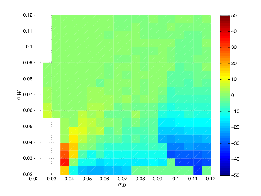
We computed the relative error between the equilibrium density of the point process, and that predicted by the moment equations with the two closures, shown in Figure 10. Panel (a) corresponds to the maxent closure and panel (b) to the power–3. We see that the maxent closure has larger relative error than the power–3 for values located below the diagonal (), which are associated with segregated spatial patterns (see Figure 9, panel (b)). In contrast, the power–3 closure performs quite well in this region. The advantage of the maxent closure becomes more noticeable on, and above the diagonal, which is associated with aggregated patterns. The ability to predict correctly the equilibrium density in this regime is nearly optimal; particularly when the two scales have similar magnitudes, even when both dispersal and mortality act over short ranges. The regions of the parameter space for which each of the two closures is relatively more useful are shown in Figure 12, which displays the difference in relative error between the two closures . Positive values of indicate that the error in the power-3 closure is larger than the maxent closure, and vice versa for negative values of . As discussed above the largest improvement of the maxent closure around to the region where the two scales are of similar magnitude.


6 Discussion
The results of this research resonate with previous work [4, 44, 53] that demonstrates that the analysis of stochastic, locally-regulated, individual-based models of population dynamics in continuous space is feasible [53, 4, 44]. The numerical implementation of the maxent closure is computationally more expensive (about twice as much) than existing closure methods, but is nonetheless faster than resorting to direct simulation of the point process; if one is willing to approximate, the simplified closure based solely on the exponential correction (49) is substantially simpler to implement, and produces very small errors in comparison with the full maxent closure. Although a number of moment closures have been proposed in the literature, some using heuristic arguments, and others based on constrained entropy maximisation, very few, if any have a criterion of validity, with the exception of Ovaskainen & Cornell [53] who were able to derive a series expansion for the mean density of a spatially explicit metapopulation problem, and show rigorously that their approximation to the mean density is exact in the limit of long range interactions. The principal benefit of the maxent method lies in the fact that the normalisation constraint used to find the domain for the correction terms fails to find a non-trivial root when the closure assumptions are not met. This situation occurs when higher order terms are required in order to fully capture the dynamics, or when correlations extend over a range that goes beyond the window of observation. This property constitutes a validation check, not present in other proposed closure schemes.
Although the power–3 or Kirkwood closure had previously been derived from maximum entropy arguments [69] (but using a different set of constraints and a different definition of the entropy functional), the correction terms presented here are new, and extend the probabilistic interpretation of the Kirkwood closure to situations where there is a region of irreducible triplet correlations. These correction terms introduce significant improvements in the agreement between the simulations of the stochastic process (for mildly aggregated patterns) and its deterministic approximation by the product density hierarchy. It remains to be seen how the maxent closure behaves for other functional forms of the interaction kernels, particularly for those that have tails that decay algebraically ( i.e. power laws) instead of exponential. Another area of further work would be related to changes in the value of the non–spatial carrying capacity . For higher densities, spatial effects become less important.
Since the derivation of the method does not depend on the details of the model, but only on that its equilibrium distribution is of maximum locational entropy with moment constraints, the maxent closure may be useful beyond spatial ecology where unclosed hierarchies for particle distribution functions are also commonly found, for instance in the statistical mechanics of fluids where the Kirkwood closure was first introduced [69], or in problems where the organisms move in space [1, 25, 78], provided that the correlation functions in those models are stationary in both space and time. A limitation of the method is its poor ability to predict the transient. This is to be expected, since maximum entropy is a meaningful property of the equilibrium distribution only when detailed balance is satisfied [74, 27, 38] and the transitions due to fecundity and dispersal events coincide with mortality.
Other areas of current and future work include the generalisation of the moment hierarchy and the maxent closure to an arbitrary order of truncation, extensions to marked spatial point processes for populations with both spatial and size structure.
Appendix. Derivation of moment equations In order to derive the equation for , we start by fixing a small region of observation (so that the count inside is either 0 or 1) and write a Master equation for the probabilities of change in the count during a small time interval , defined as
These come from the birth and death transitions. Births are given by the probability that the count increases by one in due to a birth in
This probability is controlled by the fecundity rate and the dispersal kernel,
| (61) | |||||
where is the birth rate, is the dispersal kernel, is the configuration of points at time and is the area of the 2-dimensional domain . For the death of the individual in , we have the transition
controlled by
| (62) | |||||
where and are positive constants defined in Section 2, the density–independent, and density–dependent contributions to the mortality and is the mortality kernel). This probability is conditional on there being an individual in . The change in the count is then given by both contributions
so
| (63) | |||||
Taking expectations (ensemble averaging) on both sides and dividing by the duration of a small time interval yields
after rearranging the second term, dividing both sides by and multiplying the second sum by we get
taking the limits as and go to zero, and using definition of the product density (17)
since the process is spatially stationary by construction and exploiting the fact that the dispersal kernel integrates to unity, yields
finally, after taking the limit as we get,
| (64) |
On setting , we get the the generalisation of the logistic equation to the spatial case obtained by Law & Dieckmann [43] and Law et al,law03, but derived explicitly in terms of product densities,
| (65) |
Since is unknown, we need an additional evolution equation for this object. We follow a similar procedure to that used for the mean density, but considering the expected change of the product of the counts in two observation regions and . This requires the consideration of how pairs of points are created and destroyed as individuals disperse and die. There are three possible ways in which changes to occur. The first if to fix the count and allow only to change. The second is the reverse situation, fixing and allowing only to change. The third is when both and change in a small time interval. We have that
| (66) | |||||
where the Dirac delta distribution is used to remove self-pairs. The following derivation for the second order product densities is based on the symmetry in the probabilities of a birth or a death event occurring at both extremes of the distance vector linking and . We also assume that a simultaneous change in both and is negligible
and thus the transitions of second order can be written as
| (67) |
Since we already have an expression for , given by (63), (67) becomes
Taking expectations, and dividing by both sides by gives
After dividing by and , using the definition of product densities (17) and taking the continuum limit in both space and time, one arrives at the evolution equation for the second order product density
| (68) | |||||
where we see the dependence on the third order product density in the last integral
acknowledgements
M.R acknowledges the support granted by the International Institute for Applied Systems Analysis (IIASA) to participate in the Young Scientist Summer Program where part of this research was conducted during the summer of 2004. M.R. is grateful to Richard Law who suggested to work on this problem and generously shared his time and insights, Kenneth Lindsay who kindly shared his probabilistic and simulation expertise, and fruitful discussions with Jonathan Dushoff. The authors are also grateful with Benjamin Bolker, David Murrell and David Grey who helped with details on the simulations of the point processes and generously provided access to code and manuscripts. The support of Simon A. Levin and Ioannis G. Kevrekidis is gratefully acknowledged.
References
- [1] Birch, D.A., Young, W.R.: A master equation for a spatial population model with pair interactions. Theoretical Population Biology 70(1), 26–42 (2006)
- [2] Blaszczyszyn, B.: Factorial moment expansion for stochastic systems. Stochastic Processes and their Applications 56, 321–335 (1995)
- [3] Blath, J., Etheridge, A., Meredith, M.: Coexistence in locally regulated competing populations and survival of branching annihilating random walk. The Annals of Applied Probability 17(5/6), 1474–1507 (2007)
- [4] Bolker, B., Pacala, S.W.: Using moment equations to understand stochastically driven spatial pattern formation in ecological systems. Theoretical Population Biology 52, 179–197 (1997)
- [5] Bolker, B., Pacala, S.W.: Spatial moment equations for plant competition: Understanding spatial strategies and the advantages of short dispersal. American Naturalist 153(6), 575–602 (1999)
- [6] Bolker, B., Pacala, S.W., Neuhauser, C.: Spatial dynamics in model plant communities: What do we really know. The American Naturalist 162(2), 135–148 (2003)
- [7] Bolker, B., W., P.S., Levin, S.A.: Moment methods for ecological processes in continuous space. In: U. Dieckmann, R. Law, J.A. Metz (eds.) The Geometry of Ecological Interactions, Cambridge Studies in Adaptive Dynamics, vol. 1, pp. 388–411. Cambridge University Press (2000)
- [8] Borgogno, F., D’Odorico, P., Laio, F., Ridolfi, L.: Mathematical models of vegetation pattern formation in ecohydrology. Reviews of Geophysics 47 (2009). DOI 10.1029/2007RG000256
- [9] Brooker, R.W., Maestre, F.T., Callaway, R.M., Lortie, C.L., Cavieres, L.A., Kunstler, G., Liancourt, P., Tielboerger, K., Travis, J.M.J., Anthelme, F., Armas, C., Coll, L., Corcket, E., Delzon, S., Forey, E., Kikvidze, Z., Olofsson, J., Pugnaire, F., Quiroz, C.L., Saccone, P., Schiffers, K., Seifan, M., Touzard, B., Michalet, R.: Facilitation in plant communities: the past, the present, and the future. Journal of Ecology 96(1), 18–34 (2008). DOI 10.1111/j.1365-2745.2007.01295.x
- [10] Condit, R., Ashton, P.S., Baker, P., Bunyavejchewin, S., Gunatilleke, S., Gunatilleke, N., Hubell, S.P., Foster, R., Itoh, A., LaFrankie, J.V., Seng Lee, H., Losos, E., Manokaran, N., Sukumar, R., Yamakura, T.: Spatial patterns in the distribution of tropical tree species. Science 288, 1414–1418 (2000)
- [11] Cressie, N.A.: Statistics for Spatial Data. John Wiley and Sons (1991)
- [12] Dale, M.R.: Spatial Pattern Analysis in Plant Ecology. Cambridge Studies in Ecology. Cambridge University Press (1999)
- [13] Daley, D., Vere-Jones, D.: An Introduction to the Theory of Point Processes. Springer Series in Statistics. Springer-Verlag (1988)
- [14] Daley, D., Vere-Jones, D.: An Introduction to the Theory of Point Processes. Volume I:Elementary Theory and Methods, second edn. Probability and Its Applications. Springer-Verlag (2003)
- [15] Daley, D., Vere-Jones, D.: An Introduction to the Theory of Point Processes. Volume II: General Theory and Structure, second edn. Probability and Its Applications. Springer-Verlag (2008)
- [16] Daley, D.J., Vere-Jones, D.: Scoring probability forecasts for point processes: The entropy score and information gain. Journal of Applied Probability, Special Volume 41A, 297–312 (2004)
- [17] Damgaard, C.: On the hyperbolic competition model: a comment to Weigelt et al. (2007). Journal of Ecology 95(4), 599–600 (2007). DOI 10.1111/j.1365-2745.2007.01238.x
- [18] DeAngelis, D.L., M., M.W.: Individual-based modeling of ecological and evolutionary processes. Annual Review of Ecology Evolution and Systematics 36, 147–168 (2005)
- [19] Dieckmann, U., Law, R.: Relaxation projections and the method of moments. In: U. Dieckmann, R. Law, J.A. Metz (eds.) The Geometry of Ecological Interactions, Cambridge Studies in Adaptive Dynamics, vol. 1, pp. 412–455. Cambridge University Press (2000)
- [20] Dieckmann, U., Law, R., Metz, J.A. (eds.): The Geometry of Ecological Interactions, Cambridge Studies in Adaptive dynamics, vol. 1. Cambridge University Press (2000)
- [21] Diggle, P.J.: Statistical Analysis of Spatial Point Patterns. Academic Press (1983)
- [22] Dormann, C., Roxburgh, S.: Experimental evidence rejects pairwise modelling approach to coexistence in plant communities. Proceedings of the Royal Society B-Biological Sciences 272(1569), 1279–1285 (2005). DOI 10.1098/rspb.2005.3066
- [23] Durret, R.: Stochastic spatial models. In: V. Capasso, O. Dieckmann (eds.) Mathematics Inspired by Biology, Lecture Notes in Mathematics, vol. 1714, pp. 39–94. Springer-Verlag (1999)
- [24] Etheridge, A.M.: Survival and extinction in a locally regulated population. Annals of Applied Probability 14(1), 188–214 (2004)
- [25] Flierl, H., et al.: From individuals to aggregations: The interplay between behavior and physics. Journal of Theoretical Biology 196, 397–454 (1999)
- [26] Fournier, N., Méléard, S.: A microscopic probabilistic description of a locally regulated population and macroscopic approximations. Annals of Applied Probability 14(4), 1880–1919 (2004)
- [27] Gardiner, C.: Handbook of Stochastic Methods, second edn. Springer-Verlag (1985)
- [28] Gillespie, D.: General method for numerically simulating stochastic time evolution of coupled chemical reactions. Journal of Computational Physics 22, 403–434 (1976)
- [29] Gratzer, G., Canham, C., Dieckmann, U., Fisher, A., Iwasa, Y., Law, R., Lexer, M.J., Sandmann, H., Spies, T.A., Splechtna, B.E., Szwagryzk, J.: Spatio-temporal development of forests-current trends in field methods and models. Oikos 107(1), 3–15 (2004)
- [30] Grimm, V.: Ten years of individual-based modelling in ecology:what have we learned and what could we learn in the future? Ecological Modelling 115, 129–148 (1999)
- [31] Gross, K.: Positive interactions among competitors can produce species-rich communities. Ecology Letters 11, 929–936 (2008)
- [32] Grouba, V., Zorin, A., Sevastianov, L.: The superposition approximation: A critical review. International Journal of Modern Physics B 18(1), 1–44 (2004)
- [33] Guan, Y.: A composite likelihood cross-validation approach in selecting the bandwidth for the estimation of the pair correlation function. Scandinavian Journal of Statistics 34(2), 336–346 (2007)
- [34] Guan, Y.: A least-squares cross-validation bandwidth selection approach in pair correlation function estimations. Statistics & Probability Letters 77, 1722–1729 (2007)
- [35] Hillen, T.: On the L2-moment closure of transport equations: The cattanneo approximation. Discrete and Continuous Dynamical Systems, Series B 4(4), 961–982 (2004)
- [36] Iwasa, Y.: Lattice models and pair approximations in ecology. In: U. Dieckmann, R. Law, J.A. Metz (eds.) The Geometry of Ecological Interactions, Cambridge Studies in Adaptive Dynamics, vol. 1, pp. 227–251. Cambridge University Press (2000)
- [37] Janossy, L.: On the absorption of a nucleon cascade. Proceedings of the Royal Irish Academy of Sciences, Section A 53, 181–188 (1950)
- [38] Jaynes, E.T.: Information theory and statistical mechanics. Physical Review 106(4), 620–630 (1957)
- [39] Jaynes, E.T.: On the rationale of maximum entropy methods. Proceedings of the IEEE 70(9), 939–952 (1982)
- [40] Khinchin, A.I.: Mathematical Foundations of Information Theory. Dover Publications (1957)
- [41] Kirkwood, J.G., Boggs, E.M.: The radial distribution function in liquids. Journal of Chemical Physics 10, 394–402 (1942)
- [42] Krishnarajah, I., Cook, A., Marion, G., Gibson, G.: Novel moment closure approximations in stochastic epidemics. Bulletin of Mathematical Biology 67(4), 855–873 (2005)
- [43] Law, R., Dieckmann, U.: Moment approximations of individual-based models. In: U. Dieckmann, R. Law, J.A. Metz (eds.) The Geometry of Ecological Interactions, Cambridge Studies in Adaptive dynamics, vol. 1, pp. 252–270. Cambridge University Press (2000)
- [44] Law, R., Murrell, D.J., Dieckmann, U.: Population growth in space and time: Spatial logistic equations. Ecology 84(1), 252–262 (2003)
- [45] Levin, S.A.: Patchiness in marine and terrestrial systems: from individuals to populations. Philosophical Transactions of the Royal Society of London, Series B 3, 99–103 (1994)
- [46] McFadden, J.: The entropy of a point process. Journal of the Society for Industrial and Applied Mathematics 12(4), 988–994 (1965)
- [47] Meeron, E.: Series expansion of distribution functions in multicomponent fluid systems. Journal of Chemical Physics 27(6), 1238–1246 (1957)
- [48] Moorcroft, P.R., Pacala, S.W.: A method for scaling vegetation dynamics: The ecosystem demography model. Ecological Monographs 71(4), 557–586 (2001)
- [49] Murray, J.: Mathematical Biology, Springer Series in Applied Mathematics, vol. 85. Springer-Verlag (1992)
- [50] Murray, J.D.: Mathematical Biology, Biomathematics, vol. 19. Springer-Verlag (1993)
- [51] Murrell, D., Dieckman, U., Law, R.: On moment closures for population dynamics in continuous space. Journal of Theoretical Biology 229(3), 421–432 (2004)
- [52] Othmer, H., Dunbar, S., Alt, W.: Models of dispersal in biological systems. Journal of Mathematical Biology 26, 263–298 (1988)
- [53] Ovaskainen, O., Cornell, S.J.: Asymptotically exact analysis of stochastic metapopulation dynamics with explicit spatial structure. Theoretical Population Biology 69, 13–33 (2006)
- [54] Pacala, S.W., Levin, S.A.: Biologically generated spatial pattern and the coexistence of competing species. In: D. Tilman, P. Kareiva (eds.) Spatial Ecology: The Role of Space in Populations and Interspecific Interactions, Monographs in Population Biology, vol. 30, chap. 9, pp. 204–232. Princeton University Press (1997)
- [55] Pascual, M., Levin, S.A.: From individuals to population densities: Searching for the intermediate scale of nontrivial determinism. Ecology 80(7), 2225–2236 (1999)
- [56] Pearl, R., Reed, L.: On the rate of growth of the population of the United States since 1790 and its mathematical representation. Proceedings of the National Academy of Sciences 6, 275–288 (1920)
- [57] Purves, D.W., Law, R.: Experimental derivation of functions relating growth of Arabidopsis thaliana to neighbour size and distance. Journal of Ecology 90, 882–894 (2002)
- [58] Raghib Moreno, M.: Point processes in spatial ecology. Ph.D. thesis, Department of Mathematics, University of Glasgow (2006)
- [59] Renshaw, E.: Modelling Biological Populations in Space and Time, Cambridge Studies in Mathematical Biology, vol. 11. Cambridge University Press (1991)
- [60] Salpeter, E.: On mayers theory of cluster expansion. Annals of Physics 5(3), 183–223 (1958)
- [61] Satō, K., Iwasa, Y.: Pair approximations for lattice-based ecological models. In: U. Dieckmann, R. , J.A. Metz (eds.) The Geometry of Ecological Interactions, Cambridge Studies in Adaptive Dynamics, vol. 1, pp. 341–358. Cambridge University Press (2000)
- [62] Scanlon, T.M., Caylor, K.K., Levin, S.A., Rodriguez-Iturbe, I.: Positive feedbacks promote power-law clustering of Kalahari vegetation. Nature 449(7159), 209–U4 (2007). DOI 10.1038/nature06060
- [63] Schneider, M.K., Law, R., Illian, J.B.: Quantification of neighbourhood-dependent plant growth by bayesian hierarchical modelling. Journal of Ecology 94(2), 310–321 (2006)
- [64] Scott, D.W.: Multivariate density estimation: Theory, Practice, and Visualization. Wiley series in Probability and Statistics. Wiley-Interscience (1992)
- [65] Sese, L.: Triplet correlations in the quantum hard-sphere fluid. Journal of Chemical Physics 123(10) (2005). DOI 10.1063/1.2009733
- [66] Shannon, C.E., Weaver, W.: The Mathematical Theory of Communication. University of Illinois Press (1949)
- [67] Silvertown, J., Doust, J.L.: Introduction to Plant Population Biology. Blackwell Scientific Publications (1993)
- [68] Silvertown, J., Wilson, J.B.: Spatial interactions among grassland plant populations. In: U. Dieckmann, R. Law, J.A. Metz (eds.) The Geometry of Ecological Interactions, Cambridge Studies in Adaptive Dynamics, vol. 1, pp. 28–46. Cambridge University Press (2000)
- [69] Singer, A.: Maximum entropy formulation of the Kirkwood superposition approximation. Journal of Chemical Physics 121(8), 3657–3666 (2004)
- [70] Stoll, P., Weiner, J.: A neighborhood view of interactions among individual plants. In: U. Dieckmann, R. Law, J.A. Metz (eds.) The Geometry of Ecological Interactions, Cambridge Studies in Adaptive Dynamics, vol. 1, pp. 11–27. Cambridge University Press (2000)
- [71] Stoyan, D., Helga, S.: Fractals, random shapes and point fields. Wiley (1994)
- [72] Stoyan, D., Kendall, W.S., Mecke, J.: Stochastic Geometry and its Applications, second edn. Wiley Series in Probability and Statistics. John Wiley & sons. (1995)
- [73] Turnbull, L.A., Coomes, D.A., Purves, D.W., Rees, M.: How spatial structure alters population and community dynamics in a natural plant community. Journal of Ecology 95(1), 79–89 (2007). DOI 10.1111/j.1365-2745.2006.01184.x
- [74] Van Kampen, N.: Stochastic Processes in Physics and Chemistry. North-Holland (2001)
- [75] Verhulst, P.: Notice sur la loi que la population suit dand son accroissement. Correspondence Mathematique et Physique 10, 113–121 (1838)
- [76] Weigelt, A., Schumacher, J., Walther, T., Bartelheimer, M., Steinlein, T., Beyschlag, W.: Identifying mechanisms of competition in multi-species communities. Journal of Ecology 95(1), 53–64 (2007). DOI 10.1111/j.1365-2745.2006.01198.x
- [77] Wilson, H.B., Keeling, M.J.: Spatial scales and low–dimensional deterministic dynamics. In: U. Dieckmann, R. Law, J.A. Metz (eds.) The Geometry of Ecological Interactions, Cambridge Studies in Adaptive dynamics, vol. 1, pp. 209–226. Cambridge University Press (2000)
- [78] Young, W.R., Roberts, A.J., Stuhne, G.: Reproductive pair correlations and the clustering of organisms. Nature 412, 328–331 (2001)