The Gaseous Environment of High- Galaxies:
Precision Measurements of Neutral Hydrogen
in the Circumgalactic Medium of Galaxies in the Keck Baryonic Structure Survey
Alternate Affiliation: Based on data obtained at the W.M. Keck Observatory, which is operated as a scientific partnership among the California Institute of Technology, the University of California, and the National Aeronautics and Space Administration, and was made possible by the generous financial support of the W.M. Keck Foundation.
Abstract
We present results from the Keck Baryonic Structure Survey (KBSS), a unique spectroscopic survey of the distant universe designed to explore the details of the connection between galaxies and intergalactic baryons within the same survey volumes, focusing particularly on scales from kpc to a few Mpc. The KBSS is optimized for the redshift range , combining S/N Keck/HIRES spectra of 15 of the brightest QSOs in the sky at with very densely sampled galaxy redshift surveys within a few arcmin of each QSO sightline. In this paper, we present quantitative results on the distribution, column density, kinematics, and absorber line widths of neutral hydrogen (H I) surrounding a subset of 886 KBSS star-forming galaxies with and with projected distances physical Mpc from a QSO sightline. Using Voigt profile decompositions of the full Ly forest region of all 15 QSO spectra, we compiled a catalog of individual absorbers in the redshift range of interest, with log(). These are used to measure H I absorption statistics near the redshifts of foreground galaxies as a function of projected galactocentric distance from the QSO sightline and for randomly chosen locations in the intergalactic medium (IGM) within the survey volume. We find that and the multiplicity of velocity-associated H I components increase rapidly with decreasing galactocentric impact parameter and as the systemic redshift of the galaxy is approached. The strongest H I absorbers within physical kpc of galaxies have orders of magnitude higher than those near random locations in the IGM. The circumgalactic zone of most significantly enhanced H I absorption is found within transverse distances of kpc and within km s-1 of galaxy systemic redshifts. Taking this region as the defining bounds of the circumgalactic medium (CGM), nearly half of absorbers with log() 15.5 are found within the CGM of galaxies meeting our photometric selection criteria, while their CGM occupy only 1.5% of the cosmic volume. The spatial covering fraction, multiplicity of absorption components, and characteristic remain significantly elevated to transverse distances of 2 physical Mpc from galaxies in our sample. Absorbers with cm-2 are tightly correlated with the positions of galaxies, while absorbers with lower are correlated with galaxy positions only on Mpc scales. Redshift anisotropies on these larger scales indicate coherent infall toward galaxy locations, while on scales of physical kpc peculiar velocities of km s-1 with respect to the galaxies are indicated. The median Doppler widths of individual absorbers within 1-3 of galaxies are larger by % than randomly chosen absorbers of the same , suggesting higher gas temperatures and/or increased turbulence likely caused by some combination of accretion shocks and galactic winds around galaxies with M M⊙ at .
Subject headings
cosmology: observations — galaxies: high-redshift — galaxies: evolution — galaxies: formation — intergalactic medium — quasars: absorption linesI. Introduction
Hydrogen, comprising three quarters of the baryonic mass of the universe, is the principal component of all luminous objects in the universe. It is the fuel source for stars and therefore for star formation. Thus, in order to understand the formation and evolution of galaxies, one must understand and be able to trace the inflow and outflow of this fuel.
There exist very poor observational constraints on the movement of baryons in and out of galaxies. At high redshift in star-forming systems, it has been argued that the outflow rate must be similar to the star-formation rate (Pettini et al. 2000) and that the inflow rate must be similar to the combined star-formation rate and outflow rate (Erb 2008; Finlator & Davé 2008).
Recently there has been a flurry in the theoretical literature predicting the prevalence of accretion of cold gas (log() K) onto high-z galaxies via filamentary “cold flows” (Birnboim & Dekel 2003; Kereš et al. 2005; Ocvirk et al. 2008; Brooks et al. 2009; Faucher-Giguère et al. 2011; van de Voort et al. 2011a; van de Voort et al. 2011b). In this model, the baryons stream into galaxies along the filamentary structure of the cosmic web, accreting onto galaxies without experiencing virial shocks. A wide range of predictions has been made concerning the efficiency of the transport of this material into galaxy halos, as well as its role in fueling ongoing star formation (van de Voort et al. 2011b; Faucher-Giguère et al. 2011). Further, there may be substantial suppression of the cold accretion rate caused by galaxy-scale mass outflows, evidence for which is commonly observed in the spectra of high- star-forming systems (Pettini et al. 2001; Shapley et al. 2003; Adelberger et al. 2005a; Steidel et al. 2010). Mapping the gas distribution surrounding galaxies is critical to constraining these models (Faucher-Giguère & Kereš 2011; Fumagalli et al. 2011), and would be a significant step toward understanding and quantifying the exchange of baryons between the sites of galaxy formation and the nearby intergalactic medium (IGM).
There has been a large amount of recent theoretical examination of the nature of IGM absorbers and their relation to galaxies using simulations. Ly is believed to broadly trace the filamentary large-scale structure (Cen et al. 1994; Zhang et al. 1995; Miralda-Escudé et al. 1996; Hernquist et al. 1996; Rauch et al. 1997; Theuns et al. 1998; Davé et al. 1999; Schaye 2001) although there are indications (Barnes et al. 2011) that winds could blow spatially extended halos of gas which may have recently been observed both in absorption (Steidel et al. 2010) and in Ly emission (Steidel et al. 2011). There seems to be general agreement that galactic winds are responsible for metal absorbers in the IGM. Booth et al. (2010) suggest that mostly low mass (M M⊙) galaxies must be responsible for the pollution, while Wiersma et al. (2010) suggest only half of the metals would originate from galaxies with M M⊙. Wiersma et al. (2010) also studied the history of the ejection of these metals and found that half of the metals observed at redshift 2 were ejected during the time between . Using cosmological “zoom-in” simulations Shen et al. (2011) found a “Lyman Break”-type galaxy could distribute metals to 3 virial radii by . Simcoe (2011) recently considered this problem observationally, finding that indeed 50% of the metals observed in the IGM at were placed there since , i.e. in 1.3 Gyr. Oppenheimer & Davé (2008) and Oppenheimer et al. (2010) studied the fate of winds using cosmological simulations and found that while galactic winds are likely responsible for the metallic species seen in the IGM, much of the outflowing gas may be bound to galaxies and may fall back in. In their simulations the recycling timescale scaled inversely with mass because winds emanating from more massive galaxies experienced greater hydrodynamic drag due to the increased abundance of dense IGM surrounding them. Further, in these simulations the largest source of gaseous fuel for star formation after was recycled wind material.
To date, systematic attempts to jointly study high- galaxies and their intergalactic environs have been made by Adelberger et al. (2003); Adelberger et al. (2005a) (Crighton et al. 2011, see also). These studies focused primarily on H I and C IV absorption in the spectra of background QSOs whose sightlines probed regions covered by Lyman break galaxy (LBG) surveys. This work allowed for a first glimpse of the distribution of diffuse gas surrounding forming galaxies at high redshift, and, perhaps more tantalizing, evidence for interactions between the IGM and galaxies during the epoch when galaxies are expected to be most active. Generally, Adelberger et al. (2003) and Adelberger et al. (2005a) found excess H I absorption out to h-1comoving Mpc (cMpc) of galaxies [2 physical Mpc (pMpc) at using the cosmology adopted in this paper]. C IV systems were found to correlate strongly with the positions of galaxies suggesting a causal connection. Unfortunately, these papers could not consider physical properties of the gas such as its column density or temperature because the data were not of sufficiently high quality to perform Voigt profile analysis. As such these papers focused on the transmitted flux which could be applied to a wider range of data qualities.
In this work, we provide high-accuracy analysis of the spectral regions surrounding 886 high- star-forming galaxies as seen in absorption against the spectra of background hyper-luminous QSOs using data drawn from the Keck Baryonic Structure Survey (KBSS; Steidel et al, in prep). The KBSS was specifically designed to allow for the observation of gas absorption features surrounding high-redshift star-forming galaxies, providing unique insight into the IGM/galaxy interface at high redshift. The size and quality of the KBSS sample allow us to map the distribution and properties of gas near to individual star-forming galaxies with direct physical parameters such as the column density as opposed to proxies such as the equivalent width. This paper is the first in a series designed to study the physical properties of star-forming galaxies at high redshift using Voigt profile analysis of this data sample. The complementary analysis presented by Rakic et al. (2011b) describes the pixel statistics of the QSO spectra from the KBSS and the correlation of H I optical depth with the positions and redshifts of galaxies.
In §II we discuss the galaxy and QSO data and present the Voigt profile analysis of the QSO spectra in §III. The distributions of H I absorbers as a function of velocity, impact parameter, and 3D distance are presented in §IV. In §V we consider the geometric distribution of the gas using the covering fraction and incidence of absorbers. §VI focuses on 2D “maps” of the absorber distribution around galaxies. In §VII we analyze the velocity widths of individual absorbers and their correlation with the proximity of galaxies. We discuss the results and their possible interpretation in §VIII with a brief summary of the paper and our conclusions in §IX.
Throughout this paper we assume a -CDM cosmology with km s-1 Mpc-1, , and . All distances are expressed in physical (proper) units unless stated otherwise. We use the abbreviation pkpc and pMpc to indicate physical units, and ckpc or cMpc for co-moving units. At the mean redshift of the galaxy sample (), 300 pkpc is 210h-1pkpc (physical) or h-1ckpc; the age of the universe is 2.9 Gyr, the look-back time is 10.9 Gyr, and 8.2 pkpc subtends one arcsecond on the sky.
II. Observations
The data presented in this paper are drawn from the Keck Baryonic Structure Survey (KBSS) and include a large sample of rest-UV (2188) and rest-optical (112) spectra of UV-color selected star-forming galaxies at . These galaxies were photometrically selected to lie in the foreground of one of 15 hyper-luminous QSOs in the redshift range for which we have obtained high-resolution, high signal-to-noise ratio (S/N) echelle spectra.
The redshift range of this survey has important significance in the history of the universe – it coincides with the peak of both universal star formation (Reddy et al. 2008, see ) and super-massive black hole growth (Richards et al. 2006, see ). Spectroscopic observations of star-forming galaxies during this epoch commonly exhibit signatures of strong outflowing winds (Pettini et al. 2001; Shapley et al. 2003; Adelberger et al. 2005a; Steidel et al. 2010). At the same time, the baryonic accretion rate onto galaxies is predicted to be near its peak at (e.g., van de Voort et al. 2011b; Faucher-Giguère et al. 2011; van de Voort et al. 2011a.) Thus, the signatures of galaxy formation within the IGM should be at their peak as well.
The redshift range offers a number of practical advantages as well: first, the rapidly-evolving forest has thinned enough to allow measurements of individual H I systems and to enable the detection of important metallic transitions falling in the same range (notably, O VI , 1036); second, the astrophysics-rich rest-frame far-UV becomes accessible to large ground-based telescopes equipped with state-of-the-art optical spectrographs; third, the rest-frame optical spectrum is shifted into the atmospheric transmission windows in the near infrared, allowing for observations of a suite of diagnostic emission lines (H, H, [O II] 3726,3729, [O III]4363,4959,5007, and [S II] 6717,6732) neatly packed into the J, H, and K bands.
| Name | RA | Dec | aaThe redshift of the QSO | bbThe minimum wavelength covered in the HIRES QSO spectrum | range | NgalccThe number of galaxies in our LRIS survey with 3 pMpc and spectroscopic redshifts in the correct range given in the previous column. | S/N LyddThe average signal to noise ratio per pixel of the QSO spectrum in the wavelength range pertaining to CGM Ly and Ly absorption. | S/N Ly ddThe average signal to noise ratio per pixel of the QSO spectrum in the wavelength range pertaining to CGM Ly and Ly absorption. |
|---|---|---|---|---|---|---|---|---|
| Q0100+130 (PHL957) | 01:03:11.27 | 13:16:18.2 | 2.721 | 3133 | 2.0617– 2.6838 | 47 | 77 | 50 |
| HS0105+1619 | 01:08:06.4 | 16:35:50.0 | 2.652 | 3230 | 2.1561– 2.6153 | 53 | 127 | 89 |
| Q014209 (UM673a) | 01:45:16.6 | 09:45:17.0 | 2.743 | 3097 | 2.0260– 2.7060 | 65 | 71 | 45 |
| Q0207003 (UM402) | 02:09:50.71 | 00:05:06.5 | 2.872 | 3227 | 2.1532– 2.8339 | 46 | 82 | 55 |
| Q04491645 | 04:52:14.3 | 16:40:16.2 | 2.684 | 3151 | 2.0792– 2.6470 | 50 | 73 | 41 |
| Q0821+3107 | 08:21:07.62 | 31:07:51.17 | 2.616 | 3239 | 2.1650– 2.5794 | 37 | 50 | 33 |
| Q1009+29 (CSO 38) | 10:11:55.60 | 29:41:41.7 | 2.652eeThe redshift of this QSO was revised after the fitting of the HIRES spectrum was completed. The redshift assumed for the km s-1 is 2.6395 | 3186 | 2.1132– 2.6031 | 36 | 99 | 58 |
| SBS1217+499 | 12:19:30.85 | 49:40:51.2 | 2.704 | 3098 | 2.0273– 2.6669 | 43 | 68 | 38 |
| HS1442+2931 | 14:44:53.67 | 29:19:05.6 | 2.660 | 3152 | 2.0798– 2.6237 | 46 | 99 | 47 |
| HS1549+1919 | 15:51:52.5 | 19:11:04.3 | 2.843 | 3165 | 2.0926– 2.8048 | 54 | 173 | 74 |
| HS1603+3820 | 16:04:55.38 | 38:12:01.8 | 2.551ffThe redshift of this QSO was revised after the fitting of the HIRES spectrum was completed. The redshift assumed for the km s-1 is 2.5420 | 3181 | 2.1087– 2.5066 | 37 | 108 | 58 |
| Q1623+268 (KP77) | 16:25:48.83 | 26:46:58.8 | 2.5353 | 3126 | 2.0544– 2.4999 | 133ggThe photometry and spectroscopy in fields Q1623, HS1700, and Q2343 cover larger areas than a single LRIS footprint. As such, they represent the fields in which we sample the galaxy-IGM connection at 2 pMpc. | 48 | 28 |
| HS1700+64 | 17:01:00.6 | 64:12:09.4 | 2.751 | 3138 | 2.0668– 2.7138 | 110ggThe photometry and spectroscopy in fields Q1623, HS1700, and Q2343 cover larger areas than a single LRIS footprint. As such, they represent the fields in which we sample the galaxy-IGM connection at 2 pMpc. | 98 | 42 |
| Q2206199 | 22:08:52.1 | 19:43:59.7 | 2.573 | 3084 | 2.0133– 2.5373 | 45 | 88 | 46 |
| Q2343+125 | 23:46:28.30 | 12:48:57.8 | 2.5730 | 3160 | 2.0884– 2.5373 | 84ggThe photometry and spectroscopy in fields Q1623, HS1700, and Q2343 cover larger areas than a single LRIS footprint. As such, they represent the fields in which we sample the galaxy-IGM connection at 2 pMpc. | 71 | 45 |


II.1. The Galaxy Sample
The KBSS galaxy sample, a subset of which is used in this paper (Figure 1), is described in detail by Steidel et al (2012); here we present a brief summary. Galaxies were selected for spectroscopy using their rest-frame UV colors (i.e., LBGs) according to the criteria outlined by Steidel et al. (2004) and Adelberger et al. (2004) for and by Steidel et al. (2003) for . In combination, these criteria have been devised to efficiently select star-forming galaxies over the redshift range . In total, the KBSS galaxy sample includes (5-10Å) rest-UV spectra of 2188 star-forming galaxies obtained at the W.M. Keck Observatory using the Keck 1 10m telescope and the blue arm of the Low Resolution Imaging Spectrometer (LRIS-B; Oke et al. 1995; Steidel et al. 2004.)
Most of the observations were conducted using a 400 lines mm-1 grism (blazed at 3400 Å in first order) in combination with a dichroic beamsplitter sending all light shortward of Å into the blue channel, where the wavelength coverage for a typical slit location was Å with a resolving power using 12 wide slits (Steidel et al. 2010). Some of the spectra were obtained using the d560 beamsplitter (beam divided near 5600 Å) together with a 600 lines mm-1 grism (4000 Å blaze), typically covering Å with a resolving power . Observations obtained after July 2007 made use of the Cassegrain Atmospheric Dispersion Corrector, thus minimizing the effects of differential atmospheric refraction over the spectral range of interest. Wavelength calibration was accomplished using Hg, Cd, Zn, and Ne lamps, with zero point corrections based on night sky emission lines on each individual exposure.11 1 An extensive discussion of the LRIS/KBSS wavelength calibration errors (including slit illumination and atmospheric dispersion) is given in Steidel et al. (2010).
The exposure times allocated to individual galaxies ranged from 1.5-7.5 hours depending on the number of separate masks containing the same target; typically galaxies were observed on either 1 or 2 masks, each mask receiving a total integration of 1.5 hours. Further details on the selection, observing strategy, and data reduction for KBSS galaxies are presented elsewhere (Steidel et al. 2010, Steidel et al. 2012).
The rest-UV spectra of LBGs are dominated by the continuum emission of O and B stars, over which are superposed numerous resonance absorption lines of metallic ions and H I. The H I line at 1215.67 Å may be seen in emission or absorption (and often in both). The absorption features arise in cool interstellar gas in the foreground of the OB stars; they are most commonly observed to be blue-shifted by 100 – 800 km s-1 with respect to the systemic velocity of the stars, as measured from either rest-frame optical nebular emission lines or stellar photospheric lines in stacked spectra (Pettini et al. 2001; Shapley et al. 2003; Adelberger et al. 2005a; Steidel et al. 2010, see) or from the redshift-space symmetry of Ly absorption in the nearby IGM (Rakic et al. 2011a). Common lines observed include: O VI 1031,1036, Si II , , Si II+O I (blend),Si III 1206, Si IV 1393,1402, N V 1238,1242, C II 1334, C III 977, and C IV 1548,1550. The profile of the Ly emission or absorption line is modulated by the optical depth of the material closest to the systemic velocity of the stars, which has been shown to correlate most significantly with the baryonic mass (Steidel et al. 2010) and the physical size (Law et al., in prep) of the galaxy.
The sample used in this study includes 886 galaxies within the redshift range where at minimum Ly and Ly are observed in the HIRES spectrum and with redshifts placing them at least 3000 km s-1 blue-ward of the redshift of the QSO. The latter criterion was selected to avoid proximate systems that originate within material ejected from the QSO itself and/or the region affected by its ionizing radiation field.
A typical galaxy in the spectroscopic survey has a bolometric luminosity of L⊙ (Reddy et al. 2008; Reddy et al. 2011), a star-formation rate (SFR) of M⊙ yr-1 (Erb et al. 2006b), a stellar age of Gyr (Erb et al. 2006c), and a gas-phase metallicity of (Erb et al. 2006a). The galaxies inhabit dark matter halos of average mass M⊙ (Adelberger et al. 2005b; Conroy et al. 2008, Trainor & Steidel, in prep; Rakic et al, in prep) and average dynamical masses of M⊙ (Erb et al. 2006c) and generally exhibit dispersion-dominated kinematics (Law et al. 2009). The luminous parts of the galaxies are dominated by baryons, typically half stars and half cold gas (Shapley et al. 2005; Erb et al. 2006c), with half-light radii of pkpc (Law et al. 2011). The spectroscopic sample includes objects with apparent magnitudes , where is equivalent to mAB(6830 Å). At the mean redshift of the sample () the faint limit corresponds to a galaxy of 0.25L (Reddy & Steidel 2009).
The redshift distribution of the galaxy and QSO sample is presented in Figure 1, and the distribution of physical impact parameters, , between the galaxies and the QSO lines of sight is shown in Figure 2.
At present, 112 galaxies in the full KBSS sample have been observed spectroscopically in the near-IR using using NIRSPEC (McLean et al. 1998) on the Keck II telescope. 87 of these galaxies lie in our chosen redshift interval. The NIRSPEC target selection, data, and reductions are discussed in Erb et al. (2006b); Erb et al. (2006c). The NIR redshifts, generally based on the H emission line, are estimated to be accurate to 60 km s-1 or at .
II.2. Measured and Calibrated Redshifts
Because the most prominent features in the UV spectra of star forming galaxies are not at rest with respect to a galaxy’s systemic redshift, , corrections must be applied to avoid substantial systematic redshift errors. The velocity peak and centroid of the emission line, when present, tend to be redshifted with respect to by several hundred km s-1, while the strong UV absorption features () tend to be similarly blue-shifted with respect to (Shapley et al. 2003; Adelberger et al. 2003; Steidel et al. 2010). These observations are generally interpreted as strong evidence for the presence of galaxy-scale outflows.
Here we adopt estimates of galaxy systemic redshifts () computed in the manner proposed by Adelberger et al. (2005a) and later updated by Steidel et al. (2010) and Rakic et al. (2011a). Adelberger et al. (2005a) and Steidel et al. (2010) analyzed the subset of the UV sample for which both rest-UV and rest-optical spectra had been obtained. They measured the average offset between redshifts defined by H emission versus and to estimate average corrections. The H line traces the ionized gas in star-forming regions and is therefore a reasonable proxy for the systemic velocity of the stars, which are more difficult to measure due to the weakness of the UV photospheric absorption lines. Rakic et al. (2011a) used the QSO and galaxy data set presented here and calibrated velocity offsets appropriate for various classes of LBGs by insisting that the average IGM absorption profiles should be symmetric with respect to galaxy redshifts. In both cases, the offsets represent those of the ensemble while in reality there is some scatter between individual objects even if their spectral morphology is similar. However, as we will demonstrate, the adopted must be generally quite accurate in order to produce the trends described below.
The formulae used for estimating from and measurements are reproduced below. For galaxies with H-based redshifts (87/886), we set . For galaxies which have measured with or without the presence of emission (691/886),
| (1) |
where
| (2) |
is the velocity shift needed to transform the observed redshift into its systemic value, is the measured redshift from the centroids of interstellar absorption lines, and corresponds to the estimated systemic redshift of the galaxy.
For galaxies which have redshifts measured only from Ly in emission (90/886), we compute the redshift as
| (3) |
where
| (4) |
is the velocity shift needed to transform the observed redshift into its systemic value, is the measured redshift from Ly, and is adopted systemic redshift.
For galaxies with measurements of both and , we verify that . If the corrected absorption redshift is not bracketed by the two measured redshifts (18/886 galaxies)22 2 In these cases, and have very similar values and therefore taking their average generally provides a systemic redshift with less potential error than in those galaxies for which an average shift (as in equations 1 and 3) is required., then we use the average of and :
| (5) |
The residual redshift errors have a significant impact on our ability to interpret the kinematic information in the data; thus, their amplitude will be important to consider in the examination of the line-of-sight distribution of H I. Steidel et al. (2010) found this method generally corrects the redshifts to within km s-1 of the systemic velocity.
II.3. QSO Observations
The 15 hyper-luminous () QSOs in the center of the KBSS fields (Table 1) were observed with the High Resolution Echelle Spectrometer (Vogt et al. 1994, HIRES;) on the Keck I telescope. All available archival data for these 15 QSOs have been incorporated, including data taken with UVES (Dekker et al. 2000) on the VLT for Q2206-199 and Q2343+125. We obtained additional HIRES observations in order to reach a uniformly high S/N ratio over the spectral range of primary interest, Å. The final HIRES spectra have (FWHM km s-1), S/N per pixel, covering at least the wavelength range 3100 – 6000Å with no spectral gaps. The significant improvement in the UV/blue sensitivity of HIRES resulting from a detector upgrade in 2004 enabled us to observe Ly down to at least in all 15 KBSS sightlines, and to significantly lower redshifts in many (see Table 1.) The additional constraints provided by Ly (and in many cases, additional Lyman series transitions) allow for much more accurate measurements of H I for cm-2 (see §III); this is particularly important since these column densities are typical of H I gas in the CGM at these redshifts (see §V).
The QSO spectra were reduced using T. Barlow’s MAKEE package which is specifically tailored to the reduction of HIRES data. The output from MAKEE is a wavelength-calibrated33 3 The wavelength calibration of the HIRES spectra introduce negligible error into our analysis. The HIRES spectra have calibration errors less that 0.5 km s-1. extracted spectrum of each echelle order, corrected for the echelle blaze function and transformed to vacuum, heliocentric wavelengths. The spectra were continuum-normalized in each spectral order using low-order spline interpolation, after which the normalized 2-D spectrograms were optimally combined into a single one-dimensional, continuum-normalized spectrum resampled at 2.8 km s-1 per pixel.

Three of the KBSS QSO spectra contain a damped Lyman (DLA) system ( cm-2), and three contain a sub-DLA ( cm-2). Special care must be taken in the continuum fit to the regions surrounding these systems, as the damping wings of the absorption lines extend for thousands of km s-1 from line center. In these regions, we carefully fit a Voigt profile to the core of the absorber and adjusted the original continuum fit so that the Voigt profile produced a good fit to the damping wings, as shown in the top panel of Figure 3. The final Voigt profile fit is divided into the true spectrum, resulting in a new spectrum where the wings of the DLA have been removed, as illustrated in the bottom panel of Figure 3. The re-normalized spectrum can then be used to fit additional absorption systems superposed on the damping wings.
The redshifts of the QSOs are measured from rest-frame optical emission lines using lower-dispersion NIR spectra. The details of this procedure and the expected errors in the QSO redshifts are reported upon in Trainor & Steidel (2011, submitted). The precise QSO redshifts do not affect our analysis.
III. Analysis of QSO Absorption Spectra
The process of accurately measuring H I in the forest of QSO spectra is complicated by the saturation of moderately strong absorbers and the blending of H I features with other H I or with lines of metallic species that happen to fall in the forest region.
Our analysis includes a full Voigt-profile decomposition of the Ly forest from the lowest redshift for which Ly is available in each spectrum up to km s-1 blue-ward of the QSO redshift; Table 1 shows the relevant redshift range used for each QSO in the sample. The cut-off at the high redshift end is to avoid H I systems which could be ejected from and/or ionized by the QSO itself; the low-redshift cut is necessary due to the high frequency of systems with cm-2 that will be saturated in Ly44 4 Note that the exact saturation point for the line and for any other line depends on the line width (i.e. the Doppler parameter) and thus the internal properties of the absorbing cloud.. For saturated systems, the fit to Ly is degenerate between an increase in column density or an increase in the width of the line, . The best way to resolve this degeneracy is to measure higher-order Lyman lines where decreasing oscillator strengths allow accurate determination.
Simultaneous fits were made to as many Lyman lines as were both (1) available in the observed spectral range and (2) needed to measure an unsaturated and uncontaminated profile in the highest-order line. The exact number of higher-order Lyman lines used therefore depended upon both the redshift of the absorber and the degree of contamination in the spectral region containing the higher-order Lyman series absorption features. Higher-order lines, whether saturated or unsaturated, were used whenever doing so provided additional constraints on the overall fit.
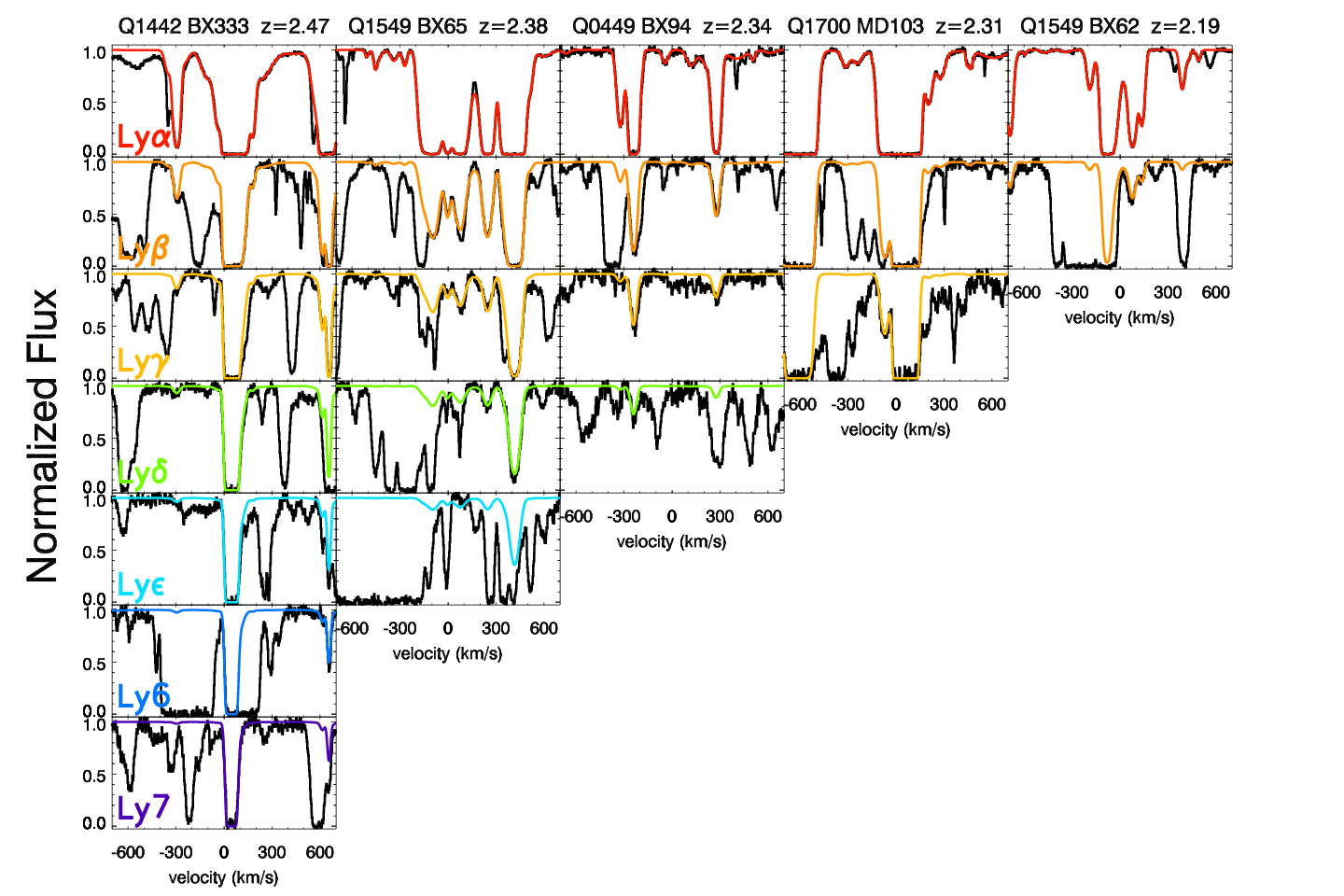
Example Voigt profile fits to the H I absorption in regions surrounding the systemic redshift of five galaxies from our sample are shown in Figure 4. Note that for galaxies with redshifts significantly larger than , many higher-order Lyman transitions can be measured.
To facilitate the fitting of the Lyman forest, we developed a semi-automatic line-fitting code. Briefly described, the code works with km s-1 sections of spectrum at a time55 5 Note, the choice of 1500 km s-1 was made largely out of convenience. This velocity window is the largest window which can be easily displayed to check the goodness of fit and for which the number of components allows for a reasonable VPFIT run time., fitting to Ly and as many higher-order lines as are accessible within the HIRES spectrum at the redshift of the H I systems being fit. The algorithm first searches for systems by cross correlating a template hydrogen absorption spectrum (i.e., a single non-saturated H I absorption component) with the HIRES spectrum. Peaks in the cross correlation are taken as initial estimates of the centroids of absorption lines. We fit Gaussians to these lines to estimate column densities and Doppler parameters. Residual absorption features (i.e., those inconsistent with ) in the Ly portion of the spectrum are assumed to be metal lines. Residual absorption in the higher-order Lyman series sections of the spectra are assumed to be lower-redshift H I systems. The fits begin with at the high-redshift end of the range so that their higher-order Lyman absorption can be flagged as a known contaminant for fitting lower-redshift H I absorbers.
Once estimates of the locations, column densities, and Doppler parameters of all the absorption lines are complete, they are input into the minimization code VPFIT66 6 http://www.ast.cam.ac.uk/ rfc/vpfit.html; © 2007 R.F. Carswell, J.K. Webb written by R.F. Carswell and J.K. Webb. VPFIT simultaneously fits all transitions of H I as well as the specified contaminating lines. The results are checked by eye, alterations made where the fit is inappropriate, and the process is repeated iteratively until a good fit (reduced ) is achieved. At this point, the multiple sections of spectrum are spliced together until a full fit to the forest is achieved.
It should be noted that the Voigt profile fit to a spectrum does not represent a unique solution. In this work, we fit each set of absorbers with the minimum number of components, adding additional components only when they significantly improve the . Median errors in reported by VPFIT are 0.07 dex for absorbers with 13 ¡ log() ¡ 14 and 0.03 dex for absorbers with 14 ¡ log() ¡ 16; however in many cases the systematic errors will exceed these values. The largest source of error in our fits to low column-density systems is uncertainty in the continuum level; for high column-density absorbers, it is the possibility of unrecognized sub-component structure.
The complete decomposition of the Ly forest in these 15 lines of sight includes Voigt profile fits to distinct H I absorption systems with cm-2, making it the largest absorber catalog ever compiled at these redshifts. It increases by an order of magnitude the number of intermediate absorbers measured with the additional constraint of higher-order Lyman lines.
IV. Circumgalactic H I


In the following sections, we discuss the statistics of individual H I absorption systems with respect to the redshifts and transverse positions of galaxies. We do not uniquely ‘‘assign’’ each absorber to a specific galaxy or vice versa. Instead we rely on comparisons between the absorption measured close to galaxies with that typical of ‘‘random’’ locations77 7 A “random” location, as described later in this section, is in effect a random redshift from our galaxy redshift catalog and an independent random position on the sky from our galaxy position catalog. in the IGM. This allows us to quantify the significance of any apparent correlation with galaxies.
In principle, it would be preferable to compare absorbers found close to galaxies with those found in IGM locations known to be far from galaxies; however, because the galaxy sample is spectroscopically incomplete compared to our photometrically selected targets,88 8 Our photometric sample is also incomplete at the faintest apparent magnitudes (Reddy et al. 2008, see), and no attempt is made to include galaxies with . we do not measure the redshifts of all galaxies in our survey volume. As a consequence, we do not know which locations in 3D space do not have a nearby galaxy. Thus, we can only compare locations near to galaxies with random locations in the IGM (irrespective of the positions of galaxies).
In order to reproduce the absorber distributions for a typical place in the IGM, we compiled a catalog of 15,000 random locations (in both redshift space and on the plane of the sky). The redshifts are drawn from the actual galaxy redshift list and therefore reproduce the typical IGM absorption associated with the redshift ranges covered by our galaxy sample. With each redshift, we also associate a randomly drawn QSO and an impact parameter to the QSO sightline from the real galaxy impact parameter list. We can then study the distribution of absorption systems around these 15,000 random locations and thereby understand how the presence of a galaxy alters the distributions.
Below we consider the distribution of H I surrounding galaxies: first along the line of sight, then on the plane of the sky, and finally as a function of 3D distance. These measurements are used to determine the relevant velocity and transverse scales of circumgalactic H I.
IV.1. Velocity-Space Distribution of H I Near Galaxies
The properties of H I gas near galaxies in our sample can be quantified in several ways. First, we consider the line of sight velocity distribution of absorbers relative to the redshifts of galaxies. Shown in Figure 5 is the velocity distribution of all absorbers with cm-2 within 1400 km s-1 in redshift and 1 pMpc in projected distance from a galaxy. We define the velocity offset, , of an absorber,
| (6) |
where is the absorption system redshift and is the adopted systemic redshift of the galaxy from §II.2. With this definition, absorbers blue-shifted with respect to galaxies have negative .


We define ,) as the number of absorbers per galaxy at a given and within the specified range of impact parameters . The solid histogram in Figure 5 represents the distribution of H I around galaxies, whereas the hatched histogram shows the average number of absorbers expected relative to randomly chosen redshifts, as described above. The number of absorbers is clearly higher near galaxies, with an excess peaking near (the galaxy systemic redshift) and confined to km s-1.
Figure 6 shows a similar pattern; in this case, each absorption system is weighted in proportion to log() such that high-column density systems contribute more significantly to the histogram. Each absorber with log() contributes [log() ] to the histogram, which is normalized by the number of galaxies considered. Taken together, Figures 5 and 6 indicate that there is an increase near galaxies of both the number and the column density of H I absorbers. The narrow peak of the distribution has an apparent half-width of 300 km s-1, while the full excess extends to km s-1 (most clearly shown in the right-hand panel of Figure 6).
As has been argued by Shapley et al. (2003); Adelberger et al. (2003); Steidel et al. (2010); Rakic et al. (2011a), these velocity distributions are also useful for checking our redshift calibration; their symmetry about km s-1 is a sensitive probe of systematic errors in our galaxy systemic redshift calibration, while the width of the distribution provides an upper limit on the random errors.99 9 The width is an upper limit because it includes both redshift errors and any peculiar velocity of absorbers relative to galaxies. A Gaussian fit to Figure 5 yields a mean with a standard deviation of km s-1.
An alternative method of quantifying the column density dependence in Figure 6 is to examine the distribution of as a function of . Figure 7 shows the median as a function of for all absorbers within pkpc of a galaxy1010 10 We choose 300 pkpc as our distance cut because the majority of the excess absorption is found within that zone, as described in §IV.2. . The asterisks indicate the median value of for each bin in velocity space. The dark vertical lines represent the dispersion in the median computed through the bootstrap method1111 11 To bootstrap the dispersion in the median, we draw (with replacement) sets of data with the same size as the real distribution. For each set the median is computed; 100 such data sets are evaluated, and then we take the 1- symmetric bounds on the distribution of the medians, i.e. the 16th and 84th percentiles.. The value of the median column density across all velocity bins for the random distribution is shown as the dark horizontal bar; the light shaded contours are the 1- bootstrapped dispersions in the median of the random sample, where we consider samples of the same size as those from the real distribution. Note that there is an enhancement by a factor of in the median out to 300 km s-1 relative to galaxy redshifts. However, for 300 km s-1, the measurements are consistent with random places in the IGM.
Shown in Figure 8 are the individual measurement of as a function of for all absorbers within 1000 km s-1 of a galaxy within pkpc of a QSO sightline. Notably, the higher- absorbers cluster strongly near the galaxy systemic redshift with a full width of km s-1.
In summary, Figures 5 8 clearly illustrate an enhancement in both the column density and number of absorption systems near the systemic velocities of galaxies. The most significant enhancement of column density is seen within 300 km s-1 (Figure 7), but there is a higher number of absorbers out to at least 700 km s-1 (Figures 5 and 6).
IV.2. Transverse Distribution of Absorbers
In addition to the strong velocity alignment of absorption systems with the systemic redshift of nearby galaxies, there is also a significant increase in the column densities, , of individual absorbers with decreasing projected (or transverse) distance between the galaxy and the line of sight, . Here, we suppose that, as an ensemble, these galaxies show similar circumgalactic absorption signatures. Therefore, because galaxies fall at various discrete impact parameters from the QSO line of sight, we can combine the information from each galaxy to make a sparsely sampled map of the absorption as a function of relative to the ensemble galaxy.
We introduce two related statistics designed to trace the change in column density as a function of . Recalling that km s-1 encompassed the bulk of the “excess” absorption (§IV.1), for each galaxy we define max(,700km s-1) to be the value of log() for the strongest absorber with 700 km s-1 of the galaxy systemic redshift. The left panel of Figure 9 shows the median value of max(,700km s-1) as a function of impact parameter. A second statistic is the logarithm of the total , sum(), of all absorbers with 700 km s-1. The statistics of the median value of sum(,700km s-1) versus is shown in the right-hand panel of Figure 9. Generally, the values of these two statistics are quite similar because the in most velocity windows is dominated by the single highest- absorber. We consider the sum because it is most easily compared to results of numerical simulations, as it does not require the fitting of Voigt profiles to simulated data and can instead be compared to a simulation “collapsed” along the line of sight.
Figure 9 clearly demonstrates that both max() and sum() increase rapidly as one approaches a galaxy. In the bin corresponding to the smallest impact parameters, pkpc, the median value of max() is more than two orders of magnitude higher than that of a random location. Moving outwards, the median value decreases with increasing to 300 pkpc, at which point the statistic “plateaus” and remains significantly higher than the random sample out to 2 pMpc. The plateau value in the galaxy-centric sample is max() cm-2, while that of the random distribution is max() cm-2. As we will discuss in §IV.2.1, max() begins to decline for pMpc.


A relevant question concerns the dependence of these statistics on the size of the velocity window considered. In Figure 9 we considered the maximum column density absorber within km s-1 of the systemic velocity of each galaxy. This corresponds to the full width of the velocity distribution shown in Figure 6. However, it is clear from Figures 6 and 7 that the majority of the excess strength of absorption falls within km s-1, especially for those systems with small impact parameters. Figure 10 shows max(,300km s-1); the trends are similar, though in the more restricted velocity window the peak on small scales is higher relative to random IGM locations–the median value in the first bin is 3 dex higher than the random redshift sample, and the extended floor of absorption is increased to at least .5 dex above the median of the random-redshift distribution. The more significant excess over random of the 300 km s-1 version is primarily due to the exclusion of unrelated absorbers at large velocity separation; however, we note that at pkpc, the differential Hubble velocity associated with this distance along the line of sight is km s-1, meaning that for large it may be more appropriate to adopt max(,700km s-1) as the relevant statistic. Regarding the sum statistic for the smaller velocity window (not shown), the value of the plateau and that of the random sample is dex higher for sum(,300 km s-1) than for max(,300 km s-1), similar to the variation in the statistics shown in Figure 9.
As we will argue in §V and §VIII.1, the velocity and spatial scales of 300 km s-1 and 300 kpc capture the most significant excess in both the column density and the number of absorbers near galaxies. In Figure 11 we provide the individual measurements max(, 300 km s-1) for all galaxies in the sample with pkpc. Note the large intrinsic scatter in max(), even at fixed impact parameter. For the 10 galaxies with the smallest impact parameters ( pkpc), the relevant portions of the QSO spectra within 1000 km s-1 of Ly at are reproduced in Figure 12.
IV.2.1 The large-scale distribution of H I
We now consider the larger-scale distribution H I around galaxies. Unfortunately, the sampling of galaxies with pMpc is comparatively poor in our sample due to the survey geometry of most of the KBSS fields (typically arcmin on the sky). This scale is imposed by the footprint of LRIS; with each field roughly centered on the bright QSO, the maximum observed impact parameter would be pMpc at . However, three out of 15 survey fields (see Table 1) were imaged with other instruments covering larger angular sizes and thus provide information on larger transverse scales. In Figures 9 and 10 we use wider bin sizes for absorbers with 1 pMpc in order to consider the large-scale distribution. This reduces the shot noise in the bins with 2 pMpc. Figures 9 and 10 demonstrate that max() remains higher than the global median value in the IGM (dark horizontal line) out to 2 pMpc, and then begins to decline. For larger , the data suggest column densities at or below that of random places in the IGM.
Again, considering the degree of scatter in max() at fixed impact parameter, Figure 13 shows max(,700km s-1) for various bins in , as indicated. The top row of panels correspond to pkpc, while the bottom two rows of panels consider larger impact parameters. Each panel shows the Kolmogorov-Smirnov probability that the two histograms are drawn from the same parent distribution. Notably, only the pMpc bins have a distribution of max() consistent with the random sample.
Thus, we have shown that the column density of H I peaks sharply at the position of galaxies in the transverse direction, that the width of the peak is pkpc, and that there remains a significant excess of H I gas to pMpc. In §VIII we discuss the implications of these results.
IV.3. 3D Distribution of
The 3D distance, , is computed using the quadrature sum of the physical impact parameter () and the line-of-sight distance calculated assuming the velocity differences are due entirely to the Hubble flow,
| (7) |
The 3D distance is therefore
| (8) |
where is given by
| (9) |
such that in our cosmology is
| (10) |
In this formalism, each absorber has a unique with respect to a galaxy in the same field.

The 3D distance, due to its strong dependence on , requires that absorbers have both small and very small values of in order to populate bins at small values of . As a result, has the effect of isolating those absorbers most likely to be associated with the galaxy without imposing a velocity cut.
Figure 14 shows that the median stays above that of an average place in the universe out to 3 pMpc.1212 12 Note, this is consistent with the quadratic sum of the extent of the velocity and transverse distance excesses seen in previous sections. The decline of as a function of is quite smooth, but again strongly peaked at the position of galaxies. The pixel analysis of the KBSS sample recently completed by Rakic et al. (2011b) studies in detail the 3D distribution of H I optical depths. There is excellent agreement between the optical depths measured in Rakic et al. (2011b) and the trends shown in Figure 14. The smoothness of the decline is caused by the shifting of absorbers with small and modest into bins at larger . Thus, the signal appearing in the inner 300 pkpc in Figure 9 is distributed across a larger number of bins in as a result of the velocity distribution of the absorbers.
The nature of the velocity width of the excess absorption will be discussed at length in §VI; however, it should be noted that all measurements of rely on the accuracy of the galaxy redshifts and in addition are affected by whatever peculiar velocities are present, whether due to random motion, inflows, or outflows.
IV.4. Connection to Galaxy-Galaxy Pair Results
Steidel et al. (2010) presented a sample of 512 close angular pairs of galaxies with different redshifts (drawn primarily from the same KBSS catalogs used in the present paper), using the spectrum of the background galaxy to probe gas associated with that in the foreground. They were able to measure the strength of absorption from H I and several metallic species over a range in impact parameter pkpc. The principal advantage of this method is that it allows for probes at very small angular separation ()–obtaining statistical results for galaxies at such small separations from QSOs is difficult due both to the “glare” of the QSO and the relative rarity of QSO-galaxy pairs with very small separations (the smallest QSO sightline–galaxy separation is pkpc or ) . As such, the galaxy pair results are highly complementary to the QSO sightline study described in this paper.
Using background galaxies instead of QSOs results in two important differences between these studies: first, background galaxies have a projected “beam size” of 1 kpc at the location of the foreground galaxy, whereas background QSOs have a projected beam of order pc. As a result, the absorption seen against background galaxies measures a combination of the covering fraction of gas on kpc scales and the column density of absorbers. Further, background galaxies are faint and therefore only low-dispersion, low-S/N spectra can be obtained. Steidel et al. (2010) thus used stacks of background galaxy spectra shifted into the rest frame of the foreground galaxies to quantify the average absorption profile surrounding these galaxies. The lower-resolution spectra do not separate into individual components as would be found in individual QSO spectra. As such, the galaxy pair method allows for the measurement of equivalent widths () only. As discussed by Steidel et al. (2010) interpretation of is complicated by its sensitivity to the covering fraction and velocity extent of the absorbing material, and its relative insensitivity to ionic column density.
Steidel et al. (2010) measured of H I, C IV, C II, Si IV, and Si II in bins of impact parameter (). The large , particularly at pkpc, seemed to require high line-of-sight velocity spread in the gas– likely higher than could be easily explained by gravitationally-induced motions, but easily accounted for by the high velocities observed “down the barrel” in the spectra of LBGs, which typically reach km s-1 for galaxies with properties similar to those in our sample.
Steidel et al. (2010) found that a simple geometric and kinematic model of outflows from LBGs could account simultaneously for the behavior of as a function of as well as the shape of the blue-shifted line profiles of strong interstellar absorption features observed along direct sightlines to the same galaxies. The presence of detected C II absorption to pkpc was cited as evidence for a non-negligible covering fraction of H I gas having cm-2 at such large galactocentric distances. Steidel et al. (2010) remarked that 90 kpc is very close to the expected virial radius for LBGs similar to those in the current sample. Our max() statistic agrees well with this inference (Figure 9); in fact, we find a covering fraction % for absorbers with cm-2 for – see § 5.
In addition, Steidel et al. (2010) used the same HIRES spectra as this work to show that the measured from the relevant portions of the high resolution spectra, averaged in the same way as the background galaxy spectra, are consistent with an extrapolation to pkpc of the trend seen in the galaxy-galaxy pairs results; a similar conclusion was reached by Rakic et al. (2011b), also using equivalent width analysis of the QSO spectra, where a smooth trend was noted out to pMpc.
IV.5. Comparison to previous studies at
Adelberger et al. (2003); Adelberger et al. (2005a) conducted the first systematic studies of high- galaxies and their surrounding IGM using sightline surveys of the IGM paired with large LBG surveys designed to probe galaxies in the same volume. Adelberger et al. (2003) analyzed the transmitted flux in the Ly forest of background QSOs, evaluated near the redshifts of survey galaxies. At the time, this was most easily accomplished using LBGs and background QSOs. These authors did not attempt Voigt profile decompositions (as in the present work) but focused on transmitted flux because it made for easier comparisons to theory and because the spectra covered the transition only, making measurements of column density or optical depth difficult due to limited dynamic range for any cm-2. Based on 8 QSO sightlines covering , Adelberger et al. (2003) found that excess H I absorption (i.e., lower transmitted flux than the average IGM at the same redshift) was present within h-1comoving Mpc (cMpc) of galaxies [1.7 physical Mpc (pMpc) at using the cosmology adopted in the present work], and an intriguing but not highly significant lack of H I very close to these galaxies (h-1cMpc or pkpc). C IV absorption was observed to be correlated with galaxy positions to out to 2.4h-1cMpc (or 800 physical kpc). The cross-correlation of C IV systems with LBGs was found to be similar to the LBG auto-correlation, suggesting that metal enriched IGM and galaxies shared the same volumes of space. The strongest C IV absorbers were so strongly correlated with LBG positions that the authors concluded that they must be causally connected to one another.

Adelberger et al. (2005a) extended similar studies to , using a larger number of QSO sightlines and a wider range of QSO spectra for the analysis. Based once again on the transmitted flux statistics, the large-scale excess near galaxies was consistent with the results of Adelberger et al. (2003), but the “turnover” of H I absorption on the smallest scales was not confirmed using the larger sample at somewhat lower redshift. Generally, the transmitted flux was decreasing with galactocentric distance, though it was still the case that % of the galaxies with the smallest impact parameters showed a lack of strong absorption, interpreted as evidence that the gas is clumpy. The results for C IV were extended, and it was shown that the correlation with galaxies grows increasingly strong as increases; the correlation length of cm-2 absorption systems was similar to that of the autocorrelation length of the galaxies. The authors attempted to correlate the observed IGM properties with galaxy properties, but no significant correlations were found given the relatively small sample of galaxies at small impact parameters.
There is no overlap in the data sample used in this paper with that of Adelberger et al. (2003) which focused on higher-redshift galaxies and QSOs. Three of the fields (Q1623, HS1700, and Q2343) included in our analysis were also included in Adelberger et al. (2005a) which considered similar redshifts to this work; however, we have increased the S/N of the QSO spectra and also added many galaxy redshifts to our catalogs for these fields since the earlier analysis. The most surprising result of the Adelberger et al. (2003) sample, especially in light of the work presented here, was the reported deficit of absorption found within 0.5 cMpc or 170 pkpc of galaxies. Adelberger et al. (2005a), with a larger data set, found that 1/3 of galaxies had relatively-little H I absorption (consistent with the pixel statistics of our sample presented in Rakic et al. 2011b), but that the majority of galaxies were associated with significant absorption. In our sample, only 1/21 galaxies with 170 pkpc has a sum(, 300 km s-1) value less than the median of the random sample. As such we concur with the argument of Adelberger et al. (2005a) suggesting that the reported deficit was due to the small sample size presented. Further, we note that a measure of shows that the majority of galaxies do have excess H I absorption in their surroundings.
On larger physical scales, Adelberger et al. (2003) and Crighton et al. (2011) considered the large-scale distribution of H I absorbers at while Adelberger et al. (2005a) studied that at . All found evidence for increased absorption to 5-6 cMpc or 2 pMpc. This scale is roughly consistent with our measurements of the 3D distribution of absorption presented in Figure 14, as well as with the trends in optical depth vs. presented in Rakic et al. (2011b).
V. The Covering Fraction and Incidence of H I

| log() rangebblog() range: The range of considered; And the incidence, , and excess probability, PE considered over three ranges of . The quoted uncertainties in and PE are calculated assuming Poisson statistics. | PE | PE | PE | |||
|---|---|---|---|---|---|---|
| [cm-2] | pMpc | pMpc | pMpc | |||
| 13.0 13.5 | 1.1 0.3 | -0.1 0.3 | 1.3 0.2 | 0.1 0.1 | 1.33 0.04 | 0.17 0.04 |
| 13.5 14.0 | 1.4 0.4 | 1.0 0.5 | 1.2 0.2 | 0.8 0.3 | 0.87 0.03 | 0.44 0.06 |
| 14.0 14.5 | 0.6 0.2 | 0.7 0.7 | 0.7 0.1 | 1.4 0.4 | 0.53 0.03 | 0.80 0.09 |
| 14.5 15.0 | 0.8 0.3 | 4.4 1.9 | 0.7 0.1 | 3.4 0.8 | 0.32 0.02 | 1.03 0.13 |
| 15.0 16.0 | 0.9 0.3 | 12.7 4.6 | 0.4 0.1 | 4.9 1.4 | 0.22 0.02 | 1.59 0.20 |
| 16.0 17.0 | 0.7 0.3 | 38.214.8 | 0.2 0.1 | 9.7 3.4 | 0.06 0.01 | 1.78 0.40 |
As discussed in §IV.1, the scale of the strongest correlation between and the positions of galaxies is found within 300 km s-1 of . Adopting this value as the characteristic velocity scale for circumgalactic gas, we can examine other useful measures of the gas distribution around galaxies. The covering fraction () and the incidence of absorbers () are two ways of quantifying the geometry of the distribution as a function of both impact parameter and .
First, we define the covering fraction, (, N0), as the fraction of galaxies in a bin of impact parameter, , that have an absorber within km s-1 with N0. This is equivalent to the geometric fraction of the area of an annulus centered on the galaxy that is covered by gas with N0 and 300 km s-1. This quantity measures the variation within the sample of the decline of as a function of .
A related quantity is the incidence of absorbers, , defined to be the number of absorbers per galaxy within a given range of and , and with km s-1. Because this quantity can be greater than unity, it has larger dynamic range and so allows for a more-complete picture of the average multiplicity of absorbers at locations close to galaxies. Also, because we consider in differential bins of , it can be used to measure the degree to which absorbers of a given associate with galaxies.1313 13 To illustrate the difference between and , suppose that all absorbers have the same . Then for a sample of two galaxies, one with 3 absorbers and the other with none, =0.5 and = 1.5.
Figure 15 illustrates the dependence of on for various thresholds of (different panels). Within 100 pkpc, even for cm-2. Also, every galaxy has an absorber with log() within 100 pkpc and km s-1. The distribution within 2.5 pMpc of lower- absorbers is relatively uniform, with 0.5. However, at larger threshold (bottom three panels) we see that is high () only within 200 pkpc. We will return to our measured values of in §5 and §V.3 where we compare our measurements to those made at low- and also to results from numerical simulations.
Figure 16 shows the average incidence of absorbers, , as a function of distance, , and ranges of (different panels). Notably, in all panels (i.e., at all columns densities) the average is higher than random for 2 pMpc. For absorbers with cm-2 (three bottom panels), there is a clear peak at small values of . No similar peak is present in the distributions of absorbers with cm-2 (top panels). Clearly absorbers with 1014.5 cm-2 are more tightly correlated with the positions of galaxies than absorbers of lower column densities.
These distributions can also be used to determine the excess probability (over that of a random place in the IGM) of intersecting an absorber of a given column density, within a range of and within some . The excess probability, PE, is defined through comparison to the random distribution:
| (11) |
Table 2 summarizes the measured values of and PE for absorbers binned in for the velocity window km s-1 and three distance cuts: pkpc, pkpc, and pMpc.

V.1. Absorbers with 1014.5 cm-2
We have shown above that absorbers with 1014.5 cm-2 appear to trace the positions of galaxies in our sample with high fidelity. The incidence of absorbers with 1014.5 cm-2 and 300 km s-1, as shown in Figure 17, nicely encapsulates the “shape” of the CGM. Similar to Figure 9 for 300 pkpc, one sees rising values of as the galactocentric distance is reduced. From 300 pkpc 2 pMpc, reaches a plateau value with 0.5 [2 pMpc = 1.4 h-1 pMpc 4.6 h-1 cMpc (at )]. For 2 pMpc, drops to values consistent with the average IGM.
Recalling the quantity P(,), defined in §IV.1 as the probability, per galaxy, of intersecting an absorber at a given and within the specified range of , here we consider the velocity distribution of absorbers with 1014.5 cm-2 in bins of as shown in Figure 18.
Fitting a Gaussian to the excess absorbers near galaxies compared to random gives a deviation () of 187 km s-1 again suggesting that the velocity scale of the excess is 300 km s-1.
Integrating the distribution in the first panel of Figure 18 corresponding to 300 kpc results in an incidence averaged over 350 km s-1 () and 300 pkpc, . Similarly, comparing the value of measured in the real and random distribution one infers that strong absorbers () are 4 times (P) more likely to be found within 300 kpc and km s-1 of a galaxy in our sample, than at a random place. The parameters of the Gaussian fits in Figure 18, as well as the inferred and PE, are listed in Table 3.
In this section, we have shown that the covering fraction, , of absorbers with log() 14.5 is roughly uniform and 0.5 out to 2 pMpc, but that those with higher only have 0.5 within 200 kpc (Figure 15). Consideration of the incidence, , indicates that absorbers with log() 14.5 are more directly related to galaxies (Figure 16). Those absorbers nicely encapsulate the “shape” of the CGM (Figure 17) and are 4 times more likely to be found within 350 km s-1 and 300 pkpc of a galaxy in our sample than at a random place in the IGM (Figure 18).

| bb:The window considered; : the Gaussian velocity centroid and its associated error; : the standard deviation of the Gaussian fit and its associated error; window: the velocity window used to compute and PE (comparable to ); : the incidence, PE: the excess probability. The quoted uncertainties in are calculated assuming Poisson statistics. The error in PE is dominated by the variation in individual realizations of the random sample: typically the variation in PE is except for the first bin (0 300 pkpc) where the variation is . | window | PE | |||
|---|---|---|---|---|---|
| [pkpc] | [km s-1] | [km s-1] | [km s-1] | ||
| 0–300 | 433 | 164 28 | -350 to 350 | 1.700.02 | 4.1 |
| 300–600 | -7450 | 253 49 | -550 to 450 | 1.070.01 | 1.19 |
| 600–900 | 2949 | 389 49 | -750 to 850 | 1.310.01 | 0.80 |
| 900–1200 | -4378 | 407 87 | -850 to 750 | 1.600.01 | 1.14 |
| 1200–1500 | 6178 | 335 80 | -650 to 750 | 1.200.01 | 0.76 |
| 1500–1800 | 4296 | 344109 | -650 to 750 | 1.060.01 | 0.63 |
V.2. Covering Fractions: Comparison with Simulations
Motivated by the desire to predict the observational signatures of cold accretion streams, two recent theoretical papers have considered the covering fraction of absorbers of various surrounding galaxies. Faucher-Giguère & Kereš (2011) consider the covering fraction of Lyman Limit (LLS, 17.2 log() 20.3) and Damped Lyman Alpha (DLA, log() 20.3) absorbers originating within cold streams near two simulated star-forming galaxies at using cosmological zoom-in simulations that do not include galactic winds. Since these authors explicitly did not consider galactic winds, their covering fractions are approximately1414 14 These values are only a lower-limit in the case that outflowing winds do not affect the gas distribution within the filamentary cold streams. van de Voort et al. (2011b) found that the wind prescription in simulations has little effect on the amount of gas that accretes onto halos but does affect the amount which is delivered into the ISM of the galaxy itself. Faucher-Giguère et al. (2011) argue that energetic winds can undergo hydrodynamical interactions with cold-streams removing some of the inflowing gas. a lower limit on the expected values. They considered a galaxy slightly less massive than those in our sample (M M⊙), as well as one comparable to those in this work (M M⊙).
For comparison, we consider the fraction of sightlines at a given for which sum(,700 km s-1) falls within the specified column density range. This is most akin to the results of Faucher-Giguère & Kereš (2011) as they measure the column density of absorbers after projecting their simulated cube onto a 2D plane. Note that here we use differential bins in (17.2 log() 20.3), and since we are considering sum() rather than max(), we use to denote the associated covering fraction (to differentiate it from the measured earlier in this section).
| Sample | log() [cm-2] | (1 ) | (2 ) |
|---|---|---|---|
| M M⊙ | 11% | ||
| 4% | |||
| M M⊙ | 12% | 4% | |
| 3% | 1% | ||
| This workaaThe tabulated here from “this work” are the fraction of galaxies with a sum() statistic in the column density range. This is subtly different from the presented earlier. Note that while we use a velocity cut of 700 km s-1 here, the results would be the same if we used a 300 km s-1 window. Had we considered as opposed to , we would have calculated 20% for the LLS covering within both 1 and 2 . The uncertainties quoted for ”this work” are 1- errors calculated assuming follows a binomial distribution. | 3014% | 249% | |
| 0%bbWe calculate the 1- upper limit on this non-detection as
where is the number of systems considered. |
44% |
Our measurements are compared with the Faucher-Giguère & Kereš (2011) simulation results in Table 4. Particularly in the case of LLS gas, we find times higher within and times higher within 2 compared with the simulations. However, if the simulations results are treated as lower limits, then clearly they are consistent with the observations.
Fumagalli et al. (2011) also considered the covering fraction of H I surrounding 6 LBG-type galaxies at using cosmological zoom-in simulations with galactic winds included (though they are relatively weak with their particular implementation). They consider absorbers within and 2 for various thresholds in log() : , , , and cm-2. A comparison with the observations is given in Table 5. The models of Fumagalli et al. (2011) clearly under-predict the presence of log() gas surrounding galaxies. Similar to Faucher-Giguère & Kereš (2011), they also seem to under predict the radial extent of gas with cm-2.
| Sample | log() [cm-2] | (1 ) | ( 2 ) |
|---|---|---|---|
| Fumagalli et al. | 38% | 22% | |
| 16% | 7% | ||
| 6% | 3% | ||
| 3% | 1% | ||
| This workaaValues in “this work” are computed as described in Table 4. Were we to consider km s-1 rather than km s-1, only the for log() 15.5 within 2 would change. The value for 300 km s-1 would be 6010%. | 909% | 689% | |
| 3014% | 289% | ||
| 109% | 85% | ||
| 0% | 44% |
V.3. Evolution of the CGM from to
| Sample | log() | ||||
|---|---|---|---|---|---|
| mÅ | [cm-2] | pkpc | km s-1 | ||
| 350 | ¡330 | 500 | 72% | ||
| ¿14 | ¡330 | 500 | 835% | ||
| 50 | 13 | ¡300 | 400 | 96% | |
| 300 | 14 | ¡300 | 400 | 70% | |
| 50 | 13 | ¡1000 | 400 | 70% | |
| 300 | 14 | ¡1000 | 400 | 38% | |
| ¿13 | ¡300 | 400 | 100%bbWe calculate the 1- lower limit on this 100% detection as
where is the number of systems considered. | ||
| ¿14 | ¡300 | 400 | 816% | ||
| ¿13 | ¡1000 | 400 | 951% | ||
| ¿14 | ¡1000 | 400 | 703% | ||
| 50 | 13 | ¡200 | 400 | 75% | |
| 50 | 13 | ¡ 400 | 400 | 81% | |
| 50 | 13 | ¡1000 | 400 | 49% | |
| 50 | 13 | ¡2000 | 400 | 48% | |
| 50 | 13 | ¡3000 | 400 | 39% | |
| 300 | 14 | ¡200 | 400 | 46% | |
| 300 | 14 | ¡400 | 400 | 44% | |
| 300 | 14 | ¡1000 | 400 | 24% | |
| 300 | 14 | ¡2000 | 400 | 22% | |
| 300 | 14 | ¡3000 | 400 | 20% | |
| 400 | 100%ccWe calculate the 1- lower limit on this 100% detection as
where is the number of systems considered. | ||||
| 400 | 982% | ||||
| 400 | 951% | ||||
| 400 | 941% | ||||
| 400 | 941% | ||||
| 400 | 925% | ||||
| 400 | 825% | ||||
| 400 | 713% | ||||
| 400 | 642% | ||||
| 400 | 612% | ||||
There have been numerous studies of the low- galaxy-IGM connection. In the interest of brevity, below we compare our measured with a small number of studies with comparable size and statistical power.

As discussed by Davé et al. (1999) and Schaye (2001), due to the expansion of the universe, the collapse of structure, and the evolution in the intensity of the metagalactic ionizing background, the associated with a fixed overdensity declines with redshift (e.g., an absorber at would have 20 times lower than would be measured at the same overdensity at ). As a consequence, absorbers with the same at different redshifts trace different structures, and have very different incidence rates. For example, there are no regions of the forest at that have zero H I absorbers in a velocity window of km s-1 – every galaxy in our sample can be associated with (generally) a large number of absorbers. This is not the case at low-, where absorption-line spectra are sparsely populated and generally galaxies would be associated with very few (possibly no) H I absorbers. Similarly, the continued growth of structure and the rapid decline in the star-formation rate density toward means that a typical low- galaxy is expected to be in a very different place on its evolutionary sequence compared to a “typical” galaxy at . Large differences are also expected for gas fractions and baryonic accretion rates at low- compared to high. Thus, one might reasonably expect circumgalactic gas to differ as well.
With these caveats in mind, we compare the covering fraction, , of the sample with results at low-.

V.3.1 The CGM at
Chen et al. (2001) considered 47 galaxies with and pkpc 1515 15 The ranges quoted here have been adjusted from the cosmology considered in Chen et al. (2001) to the cosmology used in this paper at the mean redshift of the sample, .. Their galaxy sample covered a wide range of properties, with 68% having L L. The QSO spectra used were generally not of sufficient quality to allow for Voigt profile decompositions and thus the authors measured the equivalent width () of Ly absorption. Chen et al. (2001) considered absorbers to be associated with galaxies if 500 km s-1 (Morris & Jannuzi 2006).
For mÅ ( cm-2) and pkpc, 34/47 galaxies in their sample had detectable Ly absorption, corresponding to . In the sample there are 48 galaxies with 330 pkpc. Using the same velocity window 500 km s-1, we find 40/48 (83%) have Ly absorption with cm-2, consistent with the measurements from Chen et al. (2001). For clarity, the results from the low- studies as well as our measurements are reproduced in Table 6.
V.3.2 The CGM at
Prochaska et al. (2011) studied the association of galaxies in 14 fields surrounding background QSOs. Similar to the Chen et al. (2001) study, they generally relied on conversions of published measurements into using an assumed . In total, their galaxy survey included 37 galaxies with 300 pkpc and 1200 galaxies in all with . They use a velocity window of 400 km s-1. For the 26 galaxies with L 0.1 L∗ within 300 pkpc, 25 had accompanying Ly absorption with cm-2, or 96%. In our sample, there are 43 galaxies with 300 pkpc, all of which have a cm-2 absorber within 400 km s-1 (=100%).
These values appear consistent; however, the covering fraction of cm-2 gas is a very poor measure of the extent of the CGM at high redshift. For example, if we consider the same velocity window ( 400 km s-1) and the same threshold ( cm-2), we find 95% within 1 pMpc and 94% within 2 pMpc; i.e., there is no appreciable change in the of gas of this with increasing distance. Prochaska et al. (2011) find =70% for 1 pMpc in their sample.
Measurements with a higher threshold have larger dynamic range; for cm-2, Prochaska et al. (2011) measure 70% for 300 pkpc, and 38% for 1 pMpc. For our sample, we measure % for 300 pkpc and 70% for 1 pMpc.
V.3.3 The CGM in the Local Universe: km s-1
Wakker & Savage (2009) (hereafter, WS09) studied the gaseous distribution around local galaxies ( km s-1) along 76 lines of sight. The galaxy catalog considered included local galaxies. The absorber catalog included 115 intergalactic Ly absorbers (i.e., not from the Galaxy) over the same redshift range. They calculate in cumulative distance bins (e.g. 200 pkpc).
For comparison to the WS09 sample, we use a velocity window 400 km s-1 with respect to galaxy redshifts in our high redshift sample. From WS09 (Table 10) we use the values of measured for the galaxy sample with L 0.25 L∗. 1616 16 Our spectroscopic sample includes galaxies to . This is equivalent to L 0.25 L∗ at . They consider two classes of absorbers, those with 50mÅ ( cm-2) and 300 mÅ ( cm-2). We make a direct comparison to our sample with the same threshold in Figure 19 and Table 6. Our measurements are shown in the solid histogram, the random high- sample is plotted in the (dark-blue) cross-hatched histogram, and the WS09 sample is represented by the (red) vertically-hatched histogram. One can clearly see that at all and for both thresholds in , the sample shows significantly less covering than the high- sample.
As mentioned above, absorbers of fixed are theoretically expected to trace higher-overdensity gas at low redshift than at high redshift. By considering various thresholds in our own data, we found that of the low- 50mÅ( cm-2) sample was most comparable to high- absorbers with cm-2; similarly, the WS09 300mÅ( cm-2) can be matched to our high- absorbers with cm-2. Note that we chose the threshold which best reproduced measured on Mpc scales.
These two comparisons, shown in Figure 20, exhibit remarkably similar patterns in the covering fraction of as a function of . It therefore appears that low- absorbers with log() = N0 on average trace the same physical regions around galaxies as gas with log() N at . While we do not directly measure universal overdensity, these results lend observational support to the predictions by Davé et al. (1999) and Schaye (2001) that gas at the same universal overdensity at low- and high- would have lower at low-. These measurements also suggest that the physical size of the CGM around a typical galaxy is 300 pkpc at both and .
VI. Mapping the Circumgalactic Medium


Another way to visualize the distribution of neutral hydrogen surrounding star-forming galaxies is to “map” the distribution along the transverse direction and the line of sight at the same time. As in §IV.3, we use to compute a line-of-sight distance assuming it is entirely due to the Hubble flow. In Figures 21 - 24, the vertical axes represent the velocity scale line-of-sight distribution of gas. The horizontal axes correspond to the physical impact parameter between the galaxy and the QSO line of sight, . Colors encode the incidence, , of the gas in a given pixel in the map and the black and white shading represents the signal-to-noise ratio (S/N) with which is detected.
The S/N is determined using Poisson statistics. For a given bin in and , we count the total number of absorption lines found in the random distribution, , and the number of random locations considered at that impact parameter, . We also count the number of real galaxies at that impact parameter, . The “noise” level of the map is then taken to be:
| (12) |
where the quantity inside the square root is the number of absorption systems expected (based on the incidence for the random sample) given the number of galaxies in the real sample at a given . The square root of this quantity represents the Poisson uncertainty in the number of absorbers that would be detected; the division by results in an expression for the error in per galaxy. This value is akin to the shaded error bars surrounding the median value of the random sample in Figure 9. The signal-to-noise ratio is then taken to be:
| (13) |
The maps are generated using three different bin sizes. We consider the intermediate bin size (200 x 200 pkpc) for two cuts in (Figures 21 and 23) which cover impact parameters out to 3 pMpc. For high- absorbers which exhibit a peak at small scales, we also consider maps with 100 x 100 pkpc bins (Figure 22). For low- absorbers, we provide a map with 400 x 400 pkpc bins to emphasize the large scale distribution (Figure 24). After the number of absorbers per bin is measured, the values are placed onto a 10 times finer grid and smoothed by a gaussian kernel with a full width half maximum equal to the bin size in impact parameter (x-axis) and a velocity scale of 140 km s-1 or 600 pkpc in Hubble distance (y-axis). Binning and smoothing is required to make maps of this type as the values of impact parameter and velocity are discrete. The scale of the smoothing, however, is motivated by the data. The smoothing in is selected to obtain a large enough sampling of the inner and outer bins such that the noise in the random distribution is reduced. The velocity scale smoothing corresponds roughly to the amplitude of the redshift uncertainties (see §II.2).
In Figures 21 – 24, the normalization of the color bar is re-scaled from the raw per 100 x 100, 200 x 200, or 400 x 400 pkpc bin by the multiplicative factor , where:
| (14) |
where (bin) is either 100, 200, or 400 pkpc. For the 100 pkpc bins, . This renormalization brings the scale of into agreement with that shown in Figures 16 and 17.
Recently, Rakic et al. (2011b) constructed similar maps to those presented here using pixel optical depth analysis (instead of Voigt profile fits) for a subset of the data presented here. Many of the conclusions discussed in the following section are corroborated by the independent analysis of Rakic et al. (2011b, §4).
VI.1. Absorbers with cm-2
Shown in Figure 21 is a map of for 1014.5 1017 cm-2. Here we compare a map of the absorber distribution around galaxies (left-most panel) to a map which represents the general IGM as measured using the random distribution (third panel from left). Clearly, the incidence of cm-2 absorbers is higher near galaxies than in the general IGM. remains significantly and consistently higher than that seen in the random map within 300 km s-1 along the line of sight and out to 2 pMpc in impact parameter.
The maps presented in Figure 22 which show the inner distance and velocity ranges at higher resolution, allow one to compare the scales of the absorption excess in Hubble distance and in in order to detect redshift anisotropies indicative of particular kinematic patterns. Galaxy redshift errors and peculiar velocities of gas with respect to galaxies will generally expand the line-of-sight velocity distribution.1717 17 One exception to this “rule” is the case of inflowing gas on large scales where the inflow velocities counter the relative Hubble flow causing a reduction in the line-of-sight velocity distribution. Therefore, if the signal along the line of sight is elongated more than expected given the redshift errors and the scale of the transverse distribution, the remaining velocity structure may be attributed to peculiar velocities of the gas with respect to galaxies.
Based on Figure 22, adopting the green contours as representative of the most extreme portion of the overdensity of gas (conservatively) corresponds to a velocity scale of 300 km s-1 and a physical impact parameter 125 pkpc1818 18 Maps produced using a symmetric smoothing kernel of 200 pkpc in both the line-of-sight and transverse distance (not shown) also yield excess absorption to 300 km s-1 along the line of sight. The extent of the line-of-sight distribution is robust to reductions in the line-of-sight smoothing kernel; however, the S/N associated with the excess is improved by the adopted smoothing kernel.. Subtracting in quadrature the 140 km s-1 smoothing (which corresponds roughly to our redshift errors) leaves a residual velocity scale of km s-1. This velocity, were it due to pure Hubble flow, would indicate a distance of pMpc. In order to consider the portion of the line-of-sight elongation likely due to peculiar velocities, we can subtract in quadrature the extent of the transverse distribution – in effect subtracting a possible Hubble flow broadening. Subtracting the = 125 pkpc or km s-1 leaves km s-1; in other words, peculiar velocities of 260 km s-1 are indicated by the data.1919 19 Or, we have seriously underestimated the magnitude of our galaxy redshift errors.
VI.2. Absorbers with cm-2

Figure 23 displays a map of the incidence of lower-column density absorbers (10 cm-2). Again comparing the left-most panel (galaxy positions) to the third panel from the left (random IGM), one sees that the incidence of these absorbers is higher in the regions near galaxies than in the general IGM; however, the low- map exhibits no strong peak at small galactocentric distances.
Since there is little structure on small scales in Figure 23, the map has been more heavily smoothed to emphasize larger scales. Drawing attention to the edge of the red contours in Figure 24, it appears that the scale of the excess absorption is marginally smaller along the (line-of-sight) axis (1.5 pMpc) than along the transverse distance (2 pMpc). This suggests there may be coherent infall motion on Mpc scales compressing the distribution along the line of sight, the Kaiser (1987) effect. Rakic et al. (2011b) analyze the pixel statistics in the KBSS survey and discuss the kinematics of the circumgalactic gas in detail. They find a significant detection of compression of the signal along the line of sight which they interpret as large-scale infall.
VI.3. Median Column Density Maps
An alternative visualization of the distribution of H I surrounding galaxies, avoiding the division of absorbers into low and high column density, is a map of the median in a given bin. Figure 25 shows maps where the color bar represents the median in a given bin of and . On small scales, the behavior is similar to the high- absorbers, with significant elongation in the line of sight direction, due to a combination of peculiar motions of the gas and error in .
In this section we have shown that the kinematics of absorbers with log()14.5 are consistent with a peculiar velocity component of km s-1 within pkpc of galaxies, and separately that absorbers with log()14.5 may exhibit the kinematic signature of retarded Hubble flow on scales 1 pMpc.
VI.4. Explaining the Gas-Phase Kinematics
The kinematics of the gas surrounding galaxies may provide important clues about the physical processes occurring near galaxies. The two most plausible scenarios for the origin of the observed gas is that it traces the large scale structure (in which case it is likely falling onto the halo) or that it is the result of galactic winds, known to operate in these galaxies. Most likely, it is some combination of the two phenomena. Unfortunately, the sign of the velocity offset (red-shifted or blue-shifted) cannot tell us what the relative motion of the gas is with respect to the galaxy since its position along the line of sight is not known. For example, gas which is redshifted with respect to the galaxy might be behind the galaxy, and thus be either outflowing or moving with the Hubble flow at larger distance. Conversely, redshifted absorbers could be foreground gas that is redshifted because it is falling onto the galaxy. There is no way to know a priori which scenario holds in which cases.
We recall that in §IV.1 it was shown that the full extent in spanned by absorbers comprising the net excess over random is km s-1, with the most significant portion of the excess within km s-1. Our map of high- systems confirms the 300 km s-1 excess and allows us to measure the extent of the peculiar velocities. After accounting for our estimated galaxy redshift errors (§ VI.1), the range of significant excess becomes km s-1.
In-falling cool gas is likely to be moving at relative velocities smaller than the galaxy circular velocity (Faucher-Giguère & Kereš 2011):
| (15) |
where we assume M⊙ and pkpc (see §II.1 and §VIII.3). Since we measure only the line-of-sight component of this velocity, km s-1 might serve as an approximate upper limit on the line-of-sight velocity component due to graviationally induced peculiar velocities. Unless we have significantly underestimated the measurement uncertainties in , accreting gas would be expected to have a “quieter” velocity field than observed.
On the other hand, outflows observed in the galaxy spectra regularly show blue-shifted velocities as high as 800 km s-1, and large velocity widths appear to be required to explain the strength of strongly saturated absorption at modest impact parameters ( pkpc), based on the galaxy-galaxy pairs analysis of Steidel et al. (2010). In the context of their simple model, the envelope of is simply the component of the outflow speed projected along an observers line of sight; this maximum velocity also dictates how strong the resulting absorption features will be, with increasing proportionally to . To model the behavior of with impact parameter, was the principle normalization factor and the inferred values were km s-1 depending on the ion. In the present work, the first bin in extends from 50-100 pkpc, with a median pkpc, with median log() . Assuming the Steidel et al. (2010) geometric/kinematic model (with pkpc) would predict that a line of sight with kpc would have (equivalent to an observable velocity range between and km s-1) and a threshold cm-2 [analogous to our max() statistic], both compatible with the observations from the QSO sightlines discussed above.
VII. The Doppler Width


In addition to and , the third component of a Voigt profile fit is the Doppler width, . In the case of an unsaturated line, the Voigt profile is well approximated by a Gaussian in optical depth, with a Doppler parameter:
| (16) |
In the case of purely thermal broadening, the gas temperature can be inferred directly from the Doppler parameter:
| (17) |
where is the mass of the ion and is the Boltzmann constant. For H I,
| (18) |
noting that 26 km s-1 is the median value of in the full absorber catalog.
The physical state of the IGM is predicted to be governed by the balance of two principle processes: the adiabatic cooling caused by the expansion of the Universe and photoionization heating, generally from the UV background. In the regime where this holds and in the case that the baryonic overdensity roughly traces the dark matter overdensity, a natural consequence is a relationship between the temperature of the gas, , and its density, . Higher-density regions, having more gravitational resistance to the Hubble flow, cool less and thus have higher temperatures on average (Hui & Gnedin 1997; Schaye et al. 1999, see e.g.,). And indeed, observed distributions of thermally broadened absorption lines exhibit higher for absorbers with higher (Pettini et al. 1990; Schaye et al. 2000; Bryan & Machacek 2000; Ricotti et al. 2000; McDonald et al. 2001).
Other processes can also broaden individual absorption components. For the most diffuse and physically extended absorbers, generally with lower , the Hubble flow itself can contribute significantly to the line width. Turbulence (here meaning bulk motions of the gas) can also broaden absorption features such that:
| (19) |
where is the turbulent component of the line width.
In this section we discuss the distribution of Doppler widths () observed in absorption systems as a function of their galactocentric distance. The observed trends are much more subtle than those in , but their utility in discerning the physical state of the gas motivates a careful analysis.
VII.1. The Dependence of on Proximity to Galaxies,


Figure 26 shows the Doppler width () of absorbers with cm-2 versus . While considerably more noisy than the column density trends in the previous section, it appears that within the second bin (corresponding to 100 200 pkpc) the median value of is considerably higher than that of the random sample.
We consider the trend in versus for both the sample of absorbers close to galaxies and that of the full absorber catalog. In this way, we can examine the of absorbers at fixed , as shown in Figure 27, in order to evaluate the effect of the relationship on this result. Here, each of the four closest bins in (Figure 26) is broken into individual panels. The asterisks represent the absorbers close to galaxies. The black horizontal lines and shading refer to the full absorber catalog. 2020 20 Note that within the full catalog for absorbers whose growth is expected to remain approximately linear ( cm-2, ), the median values (black horizontal lines) exhibit increasing with increasing , as one would expect for the relation. Considering first the top right-hand panel with pkpc (the bin with the majority of the signal in Figure 26) for cm-2, the median of absorbers close to galaxies is larger than the median of the full absorber sample at fixed . This suggests that the larger cannot be attributed solely to a dependence on as in the relation.
Figure 27 shows that the median for the sample of absorbers within pkpc of galaxies is systematically larger than that of absorbers from the full absorber catalogue across most bins in . However, the absorbers closest to galaxies ( 100 pkpc; top left panel of Figure 27) do not appear to exhibit the same systematic “excess” in median (cf. Figure 26). There are too few galaxies in this inner bin to determine whether the result is statistically significant.
In order to quantify the statistical significance of the apparent excess in the range pkpc, we performed a Monte Carlo simulation. This was done by drawing random samples of absorbers from the full absorber catalogue with the same distribution in and of the same size as the absorber sample close to galaxies. The figure of merit was taken to be the average difference computed as follows: in each bin of the difference between the median bd,MC from the Monte Carlo sample and the median in the full absorber catalog was computed (asterisks minus black bars in Figure 27). The differences from the bins were then averaged. The fraction of Monte Carlo samples whose average excess is greater than that of the pkpc sightline sample is 0.005, meaning the excess is significant at approximately the level.
VII.2. Doppler Widths vs. 3D Distance
In Figure 28 we consider the distribution of as a function of , which allows one to consider trends as a function of distance without pre-selecting a velocity window. Here again, is elevated for bins close to galaxies ( 400 pkpc). In the first bin, the median 35 km s-1 compared to 27 km s-1 for the random sample.
We again perform a comparison at fixed and since the median monotonically decrease with increasing , we consider cumulative distance bins. For absorbers with 600 pkpc, the median for absorbers with cm-2 is larger than the median measured in the full absorber catalog. Notably, for 15 log() 16, absorbers close to galaxies ( 400 pkpc) have a median km s-1. If interpreted as the result of an increase in gas temperature, the change in is equivalent to more than doubling . We also note that these intermediate systems that are characteristic of the CGM tend also to be associated with the strongest high ionization metals (O VI, C IV), often exhibiting evidence that the ionization has been produced by shocks in addition to photoionization (Simcoe et al. 2002).
As previously stated, the 3D distance is strongly influenced by the magnitude of . Notably, the first three bins in (those with the most significant deviation in ) correspond to absorbers with 150 km s-1.
VII.3. Doppler Parameter: Possible Physical Explanations
The trends in Doppler widths, , could have a variety of physical origins. As previously discussed, elevated could be related to the observed trend in through the relation in the IGM. However, we showed that at fixed , the median of absorbers close to galaxies is still significantly larger than in the full absorber catalog (Figures 27 and 29). This suggests that the relationship alone cannot account for the broader absorption lines close to galaxies.
Another possible contributor to increasing near galaxies is a change in the ionization at a given . If the galaxy itself produces a significant fraction of the local ionizing radiation field (i.e., in excess of that of the metagalactic UV background), then / would be smaller near galaxies. The fraction of the ionizing photons which escape the ISM of the galaxy is small (Nestor et al. 2011, Steidel et al. in prep), but their number, compared to the UV background is likely significant within 100 pkpc. In this case, the relation could hold, but the mapping of to would be altered. If this were the case, we would expect the locations of the asterisks in Figures 27 and 29 to be consistent with a leftward shift of the black bars. However, this scenario is at odds with the observation that the median of absorbers with cm-2 and 100 200 pkpc is higher than the median for any bin in observed in the full absorber catalog (Figure 27). The same is true of absorbers with 400 pkpc and cm-2 (Figure 29).
Assuming that overdensity is not the main cause of the increased , we consider other plausible processes which could lead to an increase in the temperature or turbulence of the gas. In principle it is possible to disentangle the source of the broadening (turbulent vs. thermal) by comparing the widths of absorption lines arising from ions with different atomic weights. The thermal broadening component, (T), depends on atomic mass, while the turbulent broadening component will remain constant so long as the ions reside in the same gas. While the HIRES QSO spectra in our sample include metal absorption lines which could be used for this purpose, the analysis of the metal lines is beyond the scope of this paper and will be presented elsewhere. At present, we consider the implications of both possible effects (temperature and turbulence).
Referring to Figure 28, there is an increase in the median from 27 km s-1 to 35 km s-1. Assuming purely thermal broadening, these values would indicate K and K, respectively, or an increase in temperature of 68%. If we consider the absorbers with 40 km s-1 as in Figure 29, these suggest a temperature of K. If instead the increase in line width is due to turbulence, an excess turbulent velocity of 20-30 km s-1 would account for the departure from the = 27 km s-1 global median. In either case, it is curious that the elevated Doppler widths occur in gas with 100 300 pkpc but are not detected in the bin from 0 - 100 pkpc. While the non-detection at the smallest impact parameters is likely not significant, clearly, whichever mechanism is responsible for this increase in width is acting significantly outside of the typical galaxy virial radius ( 90 pkpc).
Unless AGN are involved (galaxies with detected AGN signatures were not used in our analysis), excess photo-heating for material closer to galaxies seems unlikely, since the UV radiation field from local stellar sources is likely to be (if anything) softer than the metagalactic background believed to dominate at an average IGM location.
There are at least two plausible processes which could increase in the CGM of galaxies: galactic winds (outflows) and baryonic accretion. Accreting gas can be heated by shocks forming as the gas falls into galaxy halos. The galaxies in our sample have halo masses comparable to the theoretically expected transition mass between “cold mode” and “hot mode” accretion (van de Voort et al. 2011b; Faucher-Giguère et al. 2011; Kereš et al. 2009; Ocvirk et al. 2008); most of these authors predict that both hot and cold accretion occur in such halos at . The virial temperature for galaxies with halos of mass is expected to be K (van de Voort et al. 2011b), and Kereš et al. (2009) suggest that this hot gas may fill the volume surrounding galaxies to a few . The H I absorbers in our sample are unlikely to trace gas this hot, however gas cooling from this temperature would be detectable.
The interaction of cool dense gas with either a hot halo or a rarified wind fluid is also expected to produce turbulent boundary layers via both Rayleigh-Taylor2121 21 Rayleigh-Taylor instabilities would form in the case of a lighter, less-dense fluid lying deeper in the gravitational potential of the galaxy than a denser cold-stream. and Kelvin Helmholtz2222 22 Kelvin Helmholtz instabilities would form in the condition where the dense stream was moving with respect to the hot medium. This is especially plausible in the case of a fast moving galactic wind or a filament moving at the free-fall velocity. instabilities (Kereš & Hernquist 2009; Faucher-Giguère & Kereš 2011). These boundary layers are also where metallic ions such as O VI are expected to be most abundant.
Galactic super winds can naturally explain either thermal or turbulent broadening, potentially to large distances away from galaxies. The favored mechanism for large scale winds is shocks from supernovae which could easily increase the gas temperature of the ambient medium. Although the distance to which galactic winds propagate is not well constrained, there is evidence that they expand to at least (Steidel et al. 2010). Shen et al. (2011) recently considered high-resolution ‘‘zoom-in’’ simulations of a single Lyman Break Galaxy2323 23 Lyman Break Galaxies at have very similar properties to the galaxies studied in this paper. at . In their model, the LBG itself (as opposed to its satellite galaxies) enriches the IGM with metals from supernovae-driven winds to 3 (see their Figure 9). Kollmeier et al. (2006) considered the effect of winds on the CGM of star-forming galaxies at and found that winds could have a profound effect on the temperature of nearby gas: varying the energy released by supernovae in their simulations by a factor of 5 changed the temperature of gas close to galaxies by % (see their Figure 10). More recently, van de Voort & Schaye (2011) considered the physical properties of gas surrounding galaxies with halo masses M M⊙ at as a function of the kinematics of the gas (i.e. inflowing vs. outflowing). They found a radial temperature profile of outflowing gas qualitatively consistent with the observed increase in . Outflows are also predicted to drive gas turbulence outside of virial halos through the conversion of kinetic energy from supernova driven bubbles into random motions through gas instabilities (Evoli & Ferrara 2011, see e.g.,).
While the exact cause of the enlarged line widths is not apparent, it is clear that the physical state of the gas within 300 pkpc is markedly different from that in “random” locations in the IGM - suggesting that galaxies and their potential wells deeply affect their surrounding CGM. This fact may introduce significant complications to studies of the general IGM which will be discussed further in §VIII.5.
VIII. General Discussion
In §IV – VII we presented measurements and plausible interpretations of the properties of neutral hydrogen gas surrounding star-forming galaxies at high . Here, we speculate on the possible implications of the observed trends.
VIII.1. Gaseous “Zones” around Galaxies
The distribution of strong absorbers (Figure 9) and of the incidence of absorbers (Figures 16 and 17) suggest three distinct “zones” in the gaseous envelopes surrounding galaxies.
- 1.
The first zone corresponds to the volume within 300 pkpc. For scale, the virial radius of a typical galaxy in our sample is pkpc. Inside 300 pkpc, the values of the max() statistic are significantly elevated and rise toward the position of the galaxy (Figure 9). Figure 16 shows rising with decreasing for the three bins within 300 pkpc. Similarly, at 300 pkpc, for absorbers with drops sharply. In Figure 17, again at 300 pkpc one sees a rapid drop in the incidence of all absorbers with cm-2.
- 2.
- 3.
The third zone corresponds to 2 pMpc. The transition between the second and third zone is not a sharp feature; rather between pMpc, the distribution of absorbers as seen in the max() and statistics drops to become consistent with (or below that of) the IGM median.
Three distinct zones are also evident in the velocity distribution of absorbers.
- 1.
- 2.
- 3.
Note that in Figure 7, the median of absorbers with 300 pkpc exhibits a sharp drop-off at 300 km s-1 suggesting that absorbers at 300 pkpc are likely responsible for the excess absorption at 300 700 km s-1.
VIII.2. Defining the CGM
We adopt a working definition of the “circumgalactic medium” (CGM) as the region within 300 km s-1 and 300 pkpc of a galaxy. Figure 30 shows (in red) the fraction of absorbers from the full absorber catalog which fall within the CGM of a galaxy in our spectroscopic sample as a function of .

Our spectroscopic galaxy sample is 70% complete with respect to the photometric parent sample within 300 pkpc of the line-of-sight to the QSOs.2424 24 Our absorption line catalogue is essentially 100% complete for absorbers with log() 13. The blue histogram in Figure 30 has been corrected for this incompleteness assuming that unobserved galaxies have the same overall redshift distribution and similar CGM to those that have been observed. Figure 30 shows that 20% of all absorbers with log() 14.5 and % of those with log() arise in the CGM of galaxies that meet our selection criteria. Noting that the comoving number density of identically selected galaxies (with the same limiting magnitude of ) is cMpc-3 (Reddy et al. 2008), the CGM of LBGs at contains only % of the Universe’s volume but accounts for nearly half of the total gas cross-section for cm-2. This is perhaps surprising given that our sample includes only galaxies with and the faint-end slope of the UV luminosity function is very steep at ; however, it is consistent with previous results based on strong metal-line absorption around similar galaxies at comparable redshifts (Adelberger et al. 2003; Adelberger et al. 2005a; Steidel et al. 2010).
The situation changes substantially for cm-2; we have seen that these lower absorbers are more loosely associated with galaxies in our sample, though their incidence is enhanced by % relative to average locations in the IGM (e.g. see the top panels of Figure 16).
Stated another way, we have found that low and high- column density absorbers cluster differently with high-, UV-bright galaxies. We showed (Figure 16) that absorbers with log() exhibit a much stronger peak in incidence towards the positions of galaxies than do the absorbers with lower column densities. Similarly, in maps of the incidence (Figures 21 – 24) low-column density absorbers show only large scale correlation with the positions of galaxies while high-column density absorbers again showed a strong peak near galaxies both along the line of sight and in .
Collectively, these lines of evidence point to a circumgalactic zone defined by the boundaries of 300 km s-1 and 300 pkpc and dominated by absorbers with log() . They also suggest that only systems with log() cm-2 are confidently “IGM”– as increases beyond this limit, the likelihood that the gas lies within the CGM of a relatively bright galaxy increases very rapidly.
VIII.3. Small Scale Distribution of
In an effort to understand the physics responsible for the distribution of as a function of transverse distance from galaxies, we compare the data to two theoretical models. First we consider the possibility that the H I column density traces the dark matter halo density profile.
The typical dark matter halo hosting a galaxy in our sample is theoretically expected to follow a NFW (Navarro et al. 1997) density profile:
| (20) |
where is a normalization defined as
| (21) |
and is the critical density, is the concentration parameter of the dark matter halo which we take to be following Duffy et al. (2008), and is the virial radius for halos of average mass M⊙ (Conroy et al. 2008; Adelberger et al. 2005b, 91 pkpc; Trainor & Steidel, in prep;).

We define , the matter overdensity, as:
| (22) |
Noting the definition for the critical density:
| (23) |
we can then express the NFW profile as a function of overdensity, rather than density:
| (24) |
Using Jeans scale arguments, Schaye (2001) defined a scaling function which relates the gas overdensity () to an expected value of . While on the smallest scales where the growth is highly non-linear it is certainly not the case that is equal to , the matter overdensity (which is dominated by dark matter), the expectation is that they should mirror each other well at low overdensity () where the growth is yet to become significantly non-linear. We therefore assume , in order to compare our measured max() to theoretical density profiles. For the cosmology used in this paper, at the redshifts of our sample, the scaling function from Schaye (2001) is:
| (25) |
where is the gas temperature in units of K and is the hydrogen photoionization rate in units of s-1 where the normalization is taken from Faucher-Giguère et al. (2008). Using this relation, we can convert our max() statistic into which can then be compared to the rescaled NFW profile.
The values after converting max() to are shown in Figure 31. The (red) dashed curve is the NFW density profile (Equation 24). The NFW halo has a radial distribution similar to that of the inferred from our max() statistic for small , but falls well below the Jeans-scale-inferred overdensity for pkpc. This is expected since the NFW profile is measured in simulations for dark matter (DM) within the virial radius. In the following section, we compare to the DM density on larger scales using DM profiles drawn directly from simulations.
VIII.4. Large Scale Distribution of

Considering the distribution of gas around galaxies on Mpc scales, it is interesting to note the similarity between the scale over which circumgalactic gas has higher density than an average location in the IGM ( pMpc) and the galaxy-galaxy autocorrelation scale length recently measured from the same galaxies, cMpc ( pMpc at ; Trainor & Steidel, in prep). It would not be surprising if they were closely related.
Most of the recent work on the dark matter density profiles at several and beyond have focused on the local universe. Since we are interested in comparing the gas-inferred density profiles with an average dark matter profile at , we created median DM density profiles using the MultiDark simulation (Klypin et al. 2011). The radial density profile within 3 pMpc was computed from 100 halos with M M⊙2525 25 The halo mass was inferred from the number of particles found to “belong” to a halo using the Friends-of-Friends algorithm. The halo-mass cut of M⊙ is the same mass threshold which reproduces the clustering of galaxies in our spectroscopic sample, as described in Trainor & Steidel (in prep). The mean and median halo masses of galaxies with this halo-mass threshold are M⊙ and M⊙, respectively.. Here we consider the dark matter density profile measured in two ways presented in terms of universal overdensity as shown in Figure 31. (1) First, we consider the average density in concentric spherical shells of radius centered on the position of each halo. We take the median of this profile across the 100 halos considered (light orange dotted curve) and compare it to the max(, 300km s-1) statistic converted into overdensity using equation 25. (2) We also consider the average dark matter density profile computed within concentric cylindrical shells of radius and length km s-1 ( pkpc) as shown in the light (green) dash-dotted curve. We consider the effect of the velocity window used as well - the dark (purple) dash-dotted curve is analogous to the green curve, but with a cylinder length of 700 km s-1.
The spherically-averaged radial density profile is well-matched by the NFW profile on small scales as expected (Figure 31). After 200–300 pkpc (the same scale as the first “zone” of the CGM, §VIII.1), the spherically averaged radial density profile flattens compared with NFW. From 200–300 pkpc onwards, the inferred density declines smoothly, falling to the mean density of the universe [log()=0] at 3 pMpc.
The cylindrically averaged density profile significantly dilutes the signal in the inner bins of suggesting that the max() statistic traces more of a radial distribution than a “line-of-sight” distribution on small scales. On larger scales, the cylindrical and spherically averaged density profiles look quite similar. Between 1.5 - 2 pMpc, the two cylindrically averaged curves become consistent with each other. This suggests that on scales of 2 pMpc the density along a sightline between km s-1 and to km s-1 is similar – as one would expect far from galaxies as the density approaches the universal mean.
The density inferred from the H I measurements is markedly higher on pMpc scales than is predicted by either MultiDark DM density profile. There are three possible causes for this discrepancy: (1) It may be the case that the max() statistic traces high-density substructure while the radial density profiles drawn from the simulations are (by construction) smoothed - averaging over these structures. The assumption of Jeans smoothing intrinsic to the arguments of Schaye (2001) should minimize the discrepancy; however, it is likely still that substructure may affect our max statistics. (2) One or more of the assumptions used in the Schaye (2001) conversion between and could be invalid. For example one of the more uncertain quantities required in the conversion is the H I photoionization rate, .2626 26 refers to the photoionization rate in units of s-1. In Figure 32 we consider the change in the value of needed to bring the measured [max(, 300km s-1)] into agreement with the spherically averaged dark matter density profile. This plot suggests a normalization 40% lower than the estimates from Faucher-Giguère et al. (2008).2727 27 The temperature of the gas is another quantity that could be adjusted. The temperature assumed currently is K. To match our observations we would need to significantly lower the temperature assumed to K which is unlikely to be the case. If anything, 104 K is likely a lower limit on the temperature of the IGM at (Becker et al. 2011a, see e.g.,). (3) Another possibility is that Jeans scale arguments do not hold in detail on these scales.2828 28 We tested the agreement between the aforementioned models and our data converted using the Fluctuating Gunn-Peterson Approximation (Rauch et al. 1997, FGPA;), finding that the disagreement is larger. Rakic et al. (2011b) also compare several methods for converting between H I optical depth (akin to ) and overdensity (see their §4.5).
VIII.5. The Implications of the Distinct Physics of the CGM
The final point is a note of caution regarding the effect the CGM of luminous galaxies may have on measurements which rely on “average” locations in the IGM. In addition to the rising and observed in the CGM of galaxies, we have shown that the physical state of the absorbing gas in this region is also distinct from the general IGM. The Doppler widths, , of individual absorbers are significantly larger in the CGM zone, even when compared at fixed . Further, absorbers with cluster tightly with galaxies (Figures 16, 17, and 22), and these absorbers are found in the CGM zone with very high frequency (Figure 30).
Taken together, these observations suggest that the physics of the “IGM” which has long been leveraged for measurements varying from the metagalactic background to the matter power spectrum, may be significantly affected by the baryonic physics of galaxy formation; particularly, low-resolution IGM studies dominated by H I absorbers saturated in Ly ( cm-2) are likely to be affected by the presence of a nearby galaxy. Further observational and theoretical examination of this subject is crucial to a full understanding of the measurement power of the IGM.
In addition, studies of the distribution of metal absorption lines in the “IGM” often consider metallic species associated with HI absorbers of log() 14.5 (Cowie et al. 1995; Songaila & Cowie 1996; Ellison et al. 2000; Carswell et al. 2002; Simcoe 2011). To a large degree, this is a practical choice as the associated metal absorbers occurring in sub-solar metallicity gas must be found and measured in spectra of finite S/N. However, the properties of the CGM discussed above suggest that, as many authors have speculated, these measurements more directly probe the metallicity of the CGM than that of the IGM. Observations at generally cannot measure the associated with metal systems due to the line density of the forest, but they are likely to suffer from the same effect, adding credence to the idea that the recent discovery of the high- downturn of C IV (Ryan-Weber et al. 2006; Ryan-Weber et al. 2009; Becker et al. 2009; Becker et al. 2011b; Simcoe et al. 2011) likely also traces CGM gas.
The observations of circumgalactic and intergalactic gas and its association with forming galaxies have now progressed to the point that more stringent comparison to theoretical expectations is possible. Even using the comparatively “blunt” tool of gas covering fraction, we have shown (§5) that the distribution of HI gas around galaxies exceeds the expectations of the models to which they have been compared, with the discrepancy increasing as decreases below cm-2. It is clear that a combination of high-resolution (to capture the small-scale baryon physics) and cosmological (to provide sufficient statistical leverage) simulations will be required to make use of the more detailed physical measurements emerging from the observations: e.g., gas-phase kinematics, multi-phase velocity/density structure, redshift-space distortions, gas temperatures, turbulence, the distribution and mixing of metals, all as a function of galaxy properties. In order to match the real universe, simulations will need to realistically model the physics of feedback from star formation, supernovae, and AGN activity and its effect on gas-phase accretion from the CGM.
It will be important for future simulations to have sufficient dynamic range to make predictions about the distribution of neutral hydrogen with log() . The physical picture advocated by most modern theoretical treatments of the “IGM” is that the Ly forest traces gas of modest overdensity within the filaments of the “cosmic web”. The high covering fractions found in this study (e.g., the relatively large of saturated HI extending 2 pMpc from M⊙ dark matter halos; §V) suggest that if this picture holds, the size of these filaments may remain quite large even as they approach the positions of high-bias halos. These initial comparisons suggest that the topology of the neutral hydrogen gas may be less “filamentary” (at all column densities) than current simulations of the “cosmic web” and “cold accretion” predict. If such disagreement between simulations and observations are common and persist they may become key to a deeper understanding of the baryon physics that ultimately controls the process of galaxy formation.
IX. Summary
In this paper we have presented a detailed study of neutral hydrogen in the IGM surrounding 886 high- star-forming galaxies using spectra of background QSOs from the Keck Baryonic Structure Survey. We draw conclusions from the analysis of 15 sightlines to hyper-luminous high- QSOs using high-resolution (7 km s-1), high-signal-to-noise ratio (50-200) spectra. This study constitutes the largest absorption line catalog ever created at these redshifts through a complete Voigt profile decomposition of the Ly forest for all 15 sightlines. The high S/N and excellent UV/blue-wavelength coverage of the HIRES QSO spectra allow precise determination of the column densities of saturated H I absorption systems whose positions we have found to correlate strongly with those of the galaxies in our sample. This sample is also considered by Rakic et al. (2011b) who analyze the pixel statistics of the H I optical depth.
In this work, we study the absorption patterns of H I gas in the velocity and spatial locations surrounding each galaxy redshift. We have examined the correlations among column density (), covering fraction (), incidence (), absorption line width (), galactocentric transverse distance (), velocity offset (), and 3D distance (). Our principal results are as follows:
- 1.
The redshifts of H I absorption systems in the QSO spectra correlate strongly with the redshifts of galaxies (§IV.1). The distribution of relative velocities () is peaked at the systemic redshift of galaxies in our sample (Figure 5). The full excess absorption near galaxies falls within km s-1 with the majority of the excess (i.e. the higher column density absorbers) falling within km s-1 (Figures 6 and 7).
- 2.
The column density () of absorbers is strongly correlated with the impact parameter to a galaxy (, §IV.2). We consider the highest- absorber within km s-1 [max()] of each of the 10 galaxies within 100 physical kpc and find that the median value is 3 orders of magnitude higher than at random places in the IGM (Figure 10). A trend of rising column densities as a function of decreasing is observed within the inner 300 physical kpc (1 cMpc) surrounding galaxies (Figures 9, 10, and 11).
- 3.
The column densities () of absorbers as measured through the max() statistic plateau in the range 300 pkpc 2 pMpc (Figures 9 and 10, §IV.2.1). Interestingly, the plateau is elevated in with respect to random places in the IGM by dex. For 2 pMpc, the values of max() decline and become consistent with random places in the IGM.
- 4.
The median as a function of 3D distance2929 29 The 3D distance, , is computed using the quadratic sum of the physical impact parameter between the galaxy and the line of sight to the QSO () and the line-of-sight distance one would calculate assuming the of each absorber was due only to the Hubble flow, . smoothly declines with increasing and becomes consistent with random places in the IGM at pMpc (Figure 14, §IV.3).
- 5.
- 6.
For absorbers with log() cm-2, there is a strong peak in the incidence, , close to galaxies at 300 pkpc (Figure 16, §V). No such peak is seen in the distribution of lower-column density absorbers. This suggests that absorbers with log() cm-2 are more directly related to galaxies than absorbers of lower .
- 7.
- 8.
- 9.
Maps of the incidence, , of low and high- absorbers as a function of and allow for the measurement of redshift anisotropies (§VI). In low- gas [log() 14.5], on large scales (pMpc) the distribution along the line of sight is compressed compared to the distribution in the transverse direction. This is likely the signature of gas infall e.g. the Kaiser (1987) effect (Figure 24). In the high- gas [log() 14.5], we find the “finger of God” effect, the elongation of the distribution along the line of sight compared to the transverse distribution (Figure 22). Taking into account the effect of our redshift errors, the data are consistent with peculiar velocities of km s-1. These conclusions are in agreement with those presented in Rakic et al. (2011b) who used pixel optical depth analysis to demonstrate that the compression along the line of sight on large scales is highly significant ().
- 10.
The Doppler widths () of individual absorption lines in the HIRES spectra rise as the galactocentric distance is decreased (§VII). The majority of the increased width is found within km s-1 and 100 300 pkpc (Figures 26 and 28). The larger line widths could be caused by an increase in the gas temperature, the turbulence of the gas, or both. The median close to galaxies are consistent with a gas temperature K, or a turbulent contribution of km s-1.
- 11.
Based on these measurements, we suggest a working definition of the circumgalactic medium (CGM) to be all locations within 300 pkpc and 300 km s-1 of a galaxy. We find that the CGM of our completeness corrected galaxy sample can account for nearly half of all absorbers with log(NHI) 15.5 (Figure 30, §VIII.2). Notably, the CGM of these galaxies comprises only 1.5% of the universe’s volume at these redshifts.
These findings not only define relevant scales of the CGM of luminous galaxies at redshift , but also demonstrate that much of the moderately high- portion of the IGM likely originates in the regions surrounding luminous galaxies where the baryonic physics of galaxy formation appear to affect the physical state of the gas. This point may have important consequences for past and future studies of the “IGM” and should be considered in greater detail.
Our understanding of the physical properties of gas surrounding star-forming galaxies will greatly benefit from analysis of metallic absorption features in the HIRES spectra. These absorption lines probe the ionization state and metallicity of the gas and will provide direct constraints on the total mass in hydrogen and in metals that surround star-forming systems. This work is underway and will be published in the second paper in this series.
With this further analysis, we will have for the first time a quantitative snapshot of the baryonic interplay between the intergalactic medium and forming galaxies which is evidently central to the processes of galaxy formation and evolution.
References
- Adelberger et al. (2005a) Adelberger, K. L., Shapley, A. E., Steidel, C. C., Pettini, M., Erb, D. K., & Reddy, N. A. 2005a, ApJ, 629, 636
- Adelberger et al. (2005b) Adelberger, K. L., Steidel, C. C., Pettini, M., Shapley, A. E., Reddy, N. A., & Erb, D. K. 2005b, ApJ, 619, 697
- Adelberger et al. (2004) Adelberger, K. L., Steidel, C. C., Shapley, A. E., Hunt, M. P., Erb, D. K., Reddy, N. A., & Pettini, M. 2004, ApJ, 607, 226
- Adelberger et al. (2003) Adelberger, K. L., Steidel, C. C., Shapley, A. E., & Pettini, M. 2003, ApJ, 584, 45
- Barnes et al. (2011) Barnes, L. A., Haehnelt, M. G., Tescari, E., & Viel, M. 2011, ArXiv e-prints
- Becker et al. (2011a) Becker, G. D., Bolton, J. S., Haehnelt, M. G., & Sargent, W. L. W. 2011a, MNRAS, 410, 1096
- Becker et al. (2009) Becker, G. D., Rauch, M., & Sargent, W. L. W. 2009, ApJ, 698, 1010
- Becker et al. (2011b) Becker, G. D., Sargent, W. L. W., Rauch, M., & Calverley, A. P. 2011b, ApJ, 735, 93
- Birnboim & Dekel (2003) Birnboim, Y. & Dekel, A. 2003, MNRAS, 345, 349
- Booth et al. (2010) Booth, C. M., Schaye, J., Delgado, J. D., & Dalla Vecchia, C. 2010, ArXiv e-prints
- Brooks et al. (2009) Brooks, A. M., Governato, F., Quinn, T., Brook, C. B., & Wadsley, J. 2009, ApJ, 694, 396
- Bryan & Machacek (2000) Bryan, G. L. & Machacek, M. E. 2000, ApJ, 534, 57
- Carswell et al. (2002) Carswell, B., Schaye, J., & Kim, T. 2002, ApJ, 578, 43
- Cen et al. (1994) Cen, R., Miralda-Escudé, J., Ostriker, J. P., & Rauch, M. 1994, ApJ, 437, L9
- Chen et al. (2001) Chen, H.-W., Lanzetta, K. M., Webb, J. K., & Barcons, X. 2001, ApJ, 559, 654
- Conroy et al. (2008) Conroy, C., Shapley, A. E., Tinker, J. L., Santos, M. R., & Lemson, G. 2008, ApJ, 679, 1192
- Cowie et al. (1995) Cowie, L. L., Songaila, A., Kim, T.-S., & Hu, E. M. 1995, AJ, 109, 1522
- Crighton et al. (2011) Crighton, N. H. M., Bielby, R., Shanks, T., Infante, L., Bornancini, C. G., Bouché, N., Lambas, D. G., Lowenthal, J. D., Minniti, D., Morris, S. L., Padilla, N., Péroux, C., Petitjean, P., Theuns, T., Tummuangpak, P., Weilbacher, P. M., Wisotzki, L., & Worseck, G. 2011, MNRAS, 414, 28
- Davé et al. (1999) Davé, R., Hernquist, L., Katz, N., & Weinberg, D. H. 1999, ApJ, 511, 521
- Dekker et al. (2000) Dekker, H., D’Odorico, S., Kaufer, A., Delabre, B., & Kotzlowski, H. 2000, in Society of Photo-Optical Instrumentation Engineers (SPIE) Conference Series, Vol. 4008, Society of Photo-Optical Instrumentation Engineers (SPIE) Conference Series, ed. M. Iye & A. F. Moorwood, 534–545
- Duffy et al. (2008) Duffy, A. R., Schaye, J., Kay, S. T., & Dalla Vecchia, C. 2008, MNRAS, 390, L64
- Ellison et al. (2000) Ellison, S. L., Songaila, A., Schaye, J., & Pettini, M. 2000, AJ, 120, 1175
- Erb (2008) Erb, D. K. 2008, ApJ, 674, 151
- Erb et al. (2006a) Erb, D. K., Shapley, A. E., Pettini, M., Steidel, C. C., Reddy, N. A., & Adelberger, K. L. 2006a, ApJ, 644, 813
- Erb et al. (2006b) Erb, D. K., Steidel, C. C., Shapley, A. E., Pettini, M., Reddy, N. A., & Adelberger, K. L. 2006b, ApJ, 647, 128
- Erb et al. (2006c) —. 2006c, ApJ, 646, 107
- Evoli & Ferrara (2011) Evoli, C. & Ferrara, A. 2011, MNRAS, 413, 2721
- Faucher-Giguère & Kereš (2011) Faucher-Giguère, C.-A. & Kereš, D. 2011, MNRAS, 412, L118
- Faucher-Giguère et al. (2011) Faucher-Giguère, C.-A., Kereš, D., & Ma, C.-P. 2011, MNRAS, 1399
- Faucher-Giguère et al. (2008) Faucher-Giguère, C.-A., Lidz, A., Hernquist, L., & Zaldarriaga, M. 2008, ApJ, 688, 85
- Finlator & Davé (2008) Finlator, K. & Davé, R. 2008, MNRAS, 385, 2181
- Förster Schreiber et al. (2009) Förster Schreiber, N. M., Genzel, R., Bouché, N., Cresci, G., Davies, R., Buschkamp, P., Shapiro, K., Tacconi, L. J., Hicks, E. K. S., Genel, S., Shapley, A. E., Erb, D. K., Steidel, C. C., Lutz, D., Eisenhauer, F., Gillessen, S., Sternberg, A., Renzini, A., Cimatti, A., Daddi, E., Kurk, J., Lilly, S., Kong, X., Lehnert, M. D., Nesvadba, N., Verma, A., McCracken, H., Arimoto, N., Mignoli, M., & Onodera, M. 2009, ApJ, 706, 1364
- Fumagalli et al. (2011) Fumagalli, M., Prochaska, J. X., Kasen, D., Dekel, A., Ceverino, D., & Primack, J. R. 2011, MNRAS, 1589
- Hernquist et al. (1996) Hernquist, L., Katz, N., Weinberg, D. H., & Miralda-Escudé, J. 1996, ApJ, 457, L51+
- Hui & Gnedin (1997) Hui, L. & Gnedin, N. Y. 1997, MNRAS, 292, 27
- Kaiser (1987) Kaiser, N. 1987, MNRAS, 227, 1
- Kereš & Hernquist (2009) Kereš, D. & Hernquist, L. 2009, ApJ, 700, L1
- Kereš et al. (2009) Kereš, D., Katz, N., Davé, R., Fardal, M., & Weinberg, D. H. 2009, MNRAS, 396, 2332
- Kereš et al. (2005) Kereš, D., Katz, N., Weinberg, D. H., & Davé, R. 2005, MNRAS, 363, 2
- Klypin et al. (2011) Klypin, A. A., Trujillo-Gomez, S., & Primack, J. 2011, ApJ, 740, 102
- Kollmeier et al. (2006) Kollmeier, J. A., Miralda-Escudé, J., Cen, R., & Ostriker, J. P. 2006, ApJ, 638, 52
- Law et al. (2009) Law, D. R., Steidel, C. C., Erb, D. K., Larkin, J. E., Pettini, M., Shapley, A. E., & Wright, S. A. 2009, ApJ, 697, 2057
- Law et al. (2011) Law, D. R., Steidel, C. C., Shapley, A. E., Nagy, S. R., Reddy, N. A., & Erb, D. K. 2011, ArXiv e-prints
- McDonald et al. (2001) McDonald, P., Miralda-Escudé, J., Rauch, M., Sargent, W. L. W., Barlow, T. A., & Cen, R. 2001, ApJ, 562, 52
- McLean et al. (1998) McLean, I. S., Becklin, E. E., Bendiksen, O., Brims, G., Canfield, J., Figer, D. F., Graham, J. R., Hare, J., Lacayanga, F., Larkin, J. E., Larson, S. B., Levenson, N., Magnone, N., Teplitz, H., & Wong, W. 1998, in Society of Photo-Optical Instrumentation Engineers (SPIE) Conference Series, Vol. 3354, Society of Photo-Optical Instrumentation Engineers (SPIE) Conference Series, ed. A. M. Fowler, 566–578
- Miralda-Escudé et al. (1996) Miralda-Escudé, J., Cen, R., Ostriker, J. P., & Rauch, M. 1996, ApJ, 471, 582
- Morris & Jannuzi (2006) Morris, S. L. & Jannuzi, B. T. 2006, MNRAS, 367, 1261
- Navarro et al. (1997) Navarro, J. F., Frenk, C. S., & White, S. D. M. 1997, ApJ, 490, 493
- Nestor et al. (2011) Nestor, D. B., Shapley, A. E., Steidel, C. C., & Siana, B. 2011, ApJ, 736, 18
- Ocvirk et al. (2008) Ocvirk, P., Pichon, C., & Teyssier, R. 2008, MNRAS, 390, 1326
- Oke et al. (1995) Oke, J. B., Cohen, J. G., Carr, M., Cromer, J., Dingizian, A., Harris, F. H., Labrecque, S., Lucinio, R., Schaal, W., Epps, H., & Miller, J. 1995, PASP, 107, 375
- Oppenheimer & Davé (2008) Oppenheimer, B. D. & Davé, R. 2008, MNRAS, 387, 577
- Oppenheimer et al. (2010) Oppenheimer, B. D., Davé, R., Kereš, D., Fardal, M., Katz, N., Kollmeier, J. A., & Weinberg, D. H. 2010, MNRAS, 406, 2325
- Pettini et al. (1990) Pettini, M., Hunstead, R. W., Smith, L. J., & Mar, D. P. 1990, MNRAS, 246, 545
- Pettini et al. (2001) Pettini, M., Shapley, A. E., Steidel, C. C., Cuby, J., Dickinson, M., Moorwood, A. F. M., Adelberger, K. L., & Giavalisco, M. 2001, ApJ, 554, 981
- Pettini et al. (2000) Pettini, M., Steidel, C. C., Adelberger, K. L., Dickinson, M., & Giavalisco, M. 2000, ApJ, 528, 96
- Prochaska et al. (2011) Prochaska, J. X., Weiner, B., Chen, H. ., Mulchaey, J. S., & Cooksey, K. L. 2011, ArXiv e-prints
- Rakic et al. (2011a) Rakic, O., Schaye, J., Steidel, C. C., & Rudie, G. C. 2011a, MNRAS, 414, 3265
- Rakic et al. (2011b) —. 2011b, ArXiv e-prints
- Rauch et al. (1997) Rauch, M., Miralda-Escude, J., Sargent, W. L. W., Barlow, T. A., Weinberg, D. H., Hernquist, L., Katz, N., Cen, R., & Ostriker, J. P. 1997, ApJ, 489, 7
- Reddy et al. (2011) Reddy, N., Dickinson, M., Elbaz, D., Morrison, G., Giavalisco, M., Ivison, R., Papovich, C., Scott, D., Buat, V., Burgarella, D., Charmandaris, V., Daddi, E., Magdis, G., Murphy, E., Altieri, B., Aussel, H., Dannerbauer, H., Dasyra, K., Hwang, H. S., Kartaltepe, J., Leiton, R., Magnelli, B., & Popesso, P. 2011, ArXiv e-prints
- Reddy & Steidel (2009) Reddy, N. A. & Steidel, C. C. 2009, ApJ, 692, 778
- Reddy et al. (2008) Reddy, N. A., Steidel, C. C., Pettini, M., Adelberger, K. L., Shapley, A. E., Erb, D. K., & Dickinson, M. 2008, ApJS, 175, 48
- Richards et al. (2006) Richards, G. T., Strauss, M. A., Fan, X., Hall, P. B., Jester, S., Schneider, D. P., Vanden Berk, D. E., Stoughton, C., Anderson, S. F., Brunner, R. J., Gray, J., Gunn, J. E., Ivezić, Ž., Kirkland, M. K., Knapp, G. R., Loveday, J., Meiksin, A., Pope, A., Szalay, A. S., Thakar, A. R., Yanny, B., York, D. G., Barentine, J. C., Brewington, H. J., Brinkmann, J., Fukugita, M., Harvanek, M., Kent, S. M., Kleinman, S. J., Krzesiński, J., Long, D. C., Lupton, R. H., Nash, T., Neilsen, Jr., E. H., Nitta, A., Schlegel, D. J., & Snedden, S. A. 2006, AJ, 131, 2766
- Ricotti et al. (2000) Ricotti, M., Gnedin, N. Y., & Shull, J. M. 2000, ApJ, 534, 41
- Ryan-Weber et al. (2006) Ryan-Weber, E. V., Pettini, M., & Madau, P. 2006, MNRAS, 371, L78
- Ryan-Weber et al. (2009) Ryan-Weber, E. V., Pettini, M., Madau, P., & Zych, B. J. 2009, MNRAS, 395, 1476
- Schaye (2001) Schaye, J. 2001, ApJ, 559, 507
- Schaye et al. (1999) Schaye, J., Theuns, T., Leonard, A., & Efstathiou, G. 1999, MNRAS, 310, 57
- Schaye et al. (2000) Schaye, J., Theuns, T., Rauch, M., Efstathiou, G., & Sargent, W. L. W. 2000, MNRAS, 318, 817
- Shapley et al. (2005) Shapley, A. E., Steidel, C. C., Erb, D. K., Reddy, N. A., Adelberger, K. L., Pettini, M., Barmby, P., & Huang, J. 2005, ApJ, 626, 698
- Shapley et al. (2003) Shapley, A. E., Steidel, C. C., Pettini, M., & Adelberger, K. L. 2003, ApJ, 588, 65
- Shen et al. (2011) Shen, S., Madau, P., Aguirre, A., Guedes, J., Mayer, L., & Wadsley, J. 2011, ArXiv e-prints
- Simcoe (2011) Simcoe, R. A. 2011, ApJ, 738, 159
- Simcoe et al. (2011) Simcoe, R. A., Cooksey, K. L., Matejek, M. E., Burgasser, A. J., Bochanski, J., Lovegrove, E., Bernstein, R. A., Pipher, J. L., Forrest, W. J., McMurtry, C., Fan, X., & O’Meara, J. 2011, ArXiv e-prints
- Simcoe et al. (2002) Simcoe, R. A., Sargent, W. L. W., & Rauch, M. 2002, ApJ, 578, 737
- Songaila & Cowie (1996) Songaila, A. & Cowie, L. L. 1996, AJ, 112, 335
- Steidel et al. (2003) Steidel, C. C., Adelberger, K. L., Shapley, A. E., Pettini, M., Dickinson, M., & Giavalisco, M. 2003, ApJ, 592, 728
- Steidel et al. (2011) Steidel, C. C., Bogosavljević, M., Shapley, A. E., Kollmeier, J. A., Reddy, N. A., Erb, D. K., & Pettini, M. 2011, ArXiv e-prints
- Steidel et al. (2010) Steidel, C. C., Erb, D. K., Shapley, A. E., Pettini, M., Reddy, N., Bogosavljević, M., Rudie, G. C., & Rakic, O. 2010, ApJ, 717, 289
- Steidel et al. (2004) Steidel, C. C., Shapley, A. E., Pettini, M., Adelberger, K. L., Erb, D. K., Reddy, N. A., & Hunt, M. P. 2004, ApJ, 604, 534
- Theuns et al. (1998) Theuns, T., Leonard, A., Efstathiou, G., Pearce, F. R., & Thomas, P. A. 1998, MNRAS, 301, 478
- van de Voort & Schaye (2011) van de Voort, F. & Schaye, J. 2011, ArXiv e-prints
- van de Voort et al. (2011a) van de Voort, F., Schaye, J., Booth, C. M., & Dalla Vecchia, C. 2011a, MNRAS, 415, 2782
- van de Voort et al. (2011b) van de Voort, F., Schaye, J., Booth, C. M., Haas, M. R., & Dalla Vecchia, C. 2011b, MNRAS, 414, 2458
- Vogt et al. (1994) Vogt, S. S., Allen, S. L., Bigelow, B. C., Bresee, L., Brown, B., Cantrall, T., Conrad, A., Couture, M., Delaney, C., Epps, H. W., Hilyard, D., Hilyard, D. F., Horn, E., Jern, N., Kanto, D., Keane, M. J., Kibrick, R. I., Lewis, J. W., Osborne, J., Pardeilhan, G. H., Pfister, T., Ricketts, T., Robinson, L. B., Stover, R. J., Tucker, D., Ward, J., & Wei, M. Z. 1994, in Society of Photo-Optical Instrumentation Engineers (SPIE) Conference Series, Vol. 2198, Society of Photo-Optical Instrumentation Engineers (SPIE) Conference Series, ed. D. L. Crawford & E. R. Craine, 362–+
- Wakker & Savage (2009) Wakker, B. P. & Savage, B. D. 2009, ApJS, 182, 378
- Wiersma et al. (2010) Wiersma, R. P. C., Schaye, J., Dalla Vecchia, C., Booth, C. M., Theuns, T., & Aguirre, A. 2010, MNRAS, 409, 132
- Zhang et al. (1995) Zhang, Y., Anninos, P., & Norman, M. L. 1995, ApJ, 453, L57+