Clustering using Max-norm Constrained Optimization
Abstract
We suggest using the max-norm as a convex surrogate constraint for clustering. We show how this yields a better exact cluster recovery guarantee than previously suggested nuclear-norm relaxation, and study the effectiveness of our method, and other related convex relaxations, compared to other clustering approaches.
1 Introduction
Clustering as the problem of partitioning data into clusters with strong similarity inside the clusters and strong dissimilarity across different clusters is one of the main problems in machine learning. In this paper, we consider the problem of cut-based, or correlation, clustering [4] that has received a lot of attention recently [1, 22, 3]: Given on nodes with normalized symmetric affinity matrix (for all : and ), we want to partition into clusters so as to minimize the total disagreement
The first term, captures the internal disagreement inside clusters, and the second term captures the external agreement between nodes in different clusters. In an ideal cluster, the affinities between all members of the same cluster are and the affinities between members of two different clusters are zero and hence the objective is zero. This objective does not require the number of clusters to be known ahead of time—we may decide to use any number of clusters, and this is accounted for in the objective. Unfortunately, finding a clustering minimizing the disagreement is NP-Hard [4].
We formulate this problem as an optimization of a convex disagreement objective over a non-convex set of valid clustering matrices (Section 2) and then consider convex relaxations of this constraint. Recently, Jalali et al. [16] suggested a trace-norm (aka nuclear-norm) relaxation, casting the problem as minimizing an loss and a trace-norm penalty, and providing conditions under which the true underlying clustering is recovered. Instead of trace-norm, we propose using the max-norm (aka norm) [30], which is a tighter convex relaxation than the trace-norm. Accordingly, we establish an exact recovery guarantee for our max-norm based formulation that is strictly better then the trace-norm based guarantee. We show that if the affinity matrix is a corruption of an “ideal” clustering matrix, with a certain bound on the corruption, then the optimal solution of the max-norm bounded optimization problem is exactly the ideal clustering (Section 3.1). We also discuss even tighter convex relaxations related to the max-norm, and suggest augmenting the convex relaxation with a single-linkage post-processing step in case of non-exact recovery, showing the empirical advantages of these approaches (Section 5).
The approach we suggests relies on optimizing an objective subject to a max-norm constraint. A similar optimization problem with a trace-norm constraint (or trace-norm regularization) has recently been the subject of some interest in the context of “robust PCA” [8, 33] and recovering the structure of graphical models with latent variables [10]. As with the trace-norm regularized variant, the + max-norm problem can be formulated as an SDP and solved using standard solvers, but this is only applicable to fairly small scale problems. In Section 4, we discuss various optimization approaches to this problems, including approaches which preserve the sparsity of the solution.
1.1 Relationship to the Goemans Willimason SDP Relaxation
Our convex relaxation approach is related to the classic SDP relaxations of max-cut [13] and more generally the cut-norm [2]. In fact, if we are interested in a partition to exactly two clusters, the correlation clustering problem is essentially a max-cut problem, though with both positive and negative weights (i.e. a symmetric cut-norm problem), and our relaxation is essentially the classic SDP relaxation of these problems. Our approach and results differ in several ways.
First, we deal with problems with multiple clusters, and even when the number of clusters is not pre-determined. If the number of clusters is pre-determined, the correlation clustering problem can be written as an integer quadratic program, with a variables per node, and can be relaxed to an SDP. But this SDP will be very different from ours, and will involve a matrix of size , unlike our relaxation where the matrix is of size regardless of the number of clusters. Consequently, the rounding techniques based on (random) projections typically employed for classic SDP relaxations do not seem relevant here. Instead, we employ a single-linkage post-processing as a form of “rounding” imperfect solutions.
Second, the type of guarantees we provide are very different from those in the Theory of Computation literature. Most of the SDP relaxation work we are aware of (including the classical work cited above) focuses on worst case constant factor approximation guarantees. On one hand, this means the guarantee needs to hold even on “crazy” inputs where there is really no reasonable clustering anyway, and second, and on the other hand it is not clear how approximating the objective to within a constant factor translates to recovering an underlying clustering. Instead, we prove that when the affinity matrix is close enough to following some underlying “true” clustering, the true clustering will be recovered exactly. This type of guarantee is more in the spirit of compressed sensing, which where exact recovery of a support set is guaranteed subject to conditions on the input [16].
1.2 Other Clustering Approaches
There are several classes of clustering algorithms with different objectives. In hierarchical clustering algorithms such as UPGMA [28], SLINK [27] and CLINK [11] the goal is to generate a sequence of clusterings by produce a sequence of clustering by merging/splitting two clusters at each step of the sequence according to a local disagreement objective as opposed to our global . Because of this locality, these methods are known to be very sensetive to outliers.
Cut-based clustering algorithms such as -means/medians [31, 15], ratio association [26], ratio cut [9] and normalized cut [34] try to optimize an objective function globally. The main issue with these objectives is that they are typically NP-Hard and need to know the number of clusters ahead of time, since these objectives are monotone in the number of clusters.
In contrast, spectral clustering algorithms[32] try to find the first principal component of the affinity matrix or a transformed version of that [24]. These methods require the number of clusters in advance and has been shown to be tractable (convex) relaxations to NP-Hard cut-based algorithms [12]. These methods are again very sensitive to outliers as they might change the principal components dramatically.
2 Problem Setup
Our approach is based on representing a clustering through its incidence matrix where iff and belong to the same cluster in (i.e. for some ), and otherwise (i.e. if and belong to different clusters). The matrix is thus a permuted block-diagonal matrix, and can also be thought of as the edge incidence matrix of a graph with cliques corresponding to clusters in . We will say that a matrix is a valid clustering matrix, or sometimes simply valid, if it can be written as for some clustering (i.e. if it is a permuted block diagonal matrix, with s in the diagonal blocks).
The disagreement can then be written as either:
| (1) |
or as:
| (2) |
where the term does not depend on the clustering and can thus be dropped.
We now phrase the correlation clustering problem as matrix problem, where we would like to solve
| (3) |
The problem is that even though the objectives (1) and (2) are convex, the constraint that is valid is certainly not constraint. Our approach to correlation clustering will thus be to relax this non-convex constraint (the validity of ) to a convex constraint.
We note that although both the absolute error objective (1) and the linear objective (2) agree on valid clustering matrices (or more generally, on binary matrices ), they can differ when is fractional, and especially when is also fractional. The choice of objective can thus be important when relaxing the validity constraint to a convex constraint. More specifically, as long as is binary (i.e. ), and , even if is fractional, the two objectives agree. Non-negativity of is ensured in some, but not all, of the convex relaxations we study. When non-negativity is not ensured, the absolute error objective (1) would tend to avoid negative values, but the linear objective might certainly prefer them. More importantly, once the affinities are also fractional, the two objectives differ even for . While the linear objective would tend to not care much about entries with affinities close to , the absolute error objective would tend to encourage fractional values in thees cases.
The linear objective also has some optimization advantages over the absolute function as well. From a numerical optimization point of view, dealing with the linear objective function is easier since we do not need to compute the sub-gradients of the -norm.
3 Max-Norm Relaxation
As discussed in the previous Section, we are interested in optimizing over the non-convex set of valid clustering matrices. The approach we discuss here is to relaxing this set to the set of matrices with bounded max-norm [30]. The max-norm of a matrix is defined as
where, is the maximum of the norm of the rows, and the minimization is over factorization of any internal dimensionality. It is not hard to see that if is a valid clustering matrix, with , then . This is achieved, e.g., by a factorization with , and where each row of is a (unit norm) indicator vector with for and zero elsewhere.
Relaxing the validity constraint to a max-norm constraint, and using the absolute error objective, we obtain the following convex relaxation of the correlation clustering problem:
| (4) |
Alternatively, we could have used the linear objective (2) instead. In any case, after finding , it is easy to check whether it is valid, and if so recover the clustering from its block structure. If is valid, we are assured the corresponding clustering is a globally optimal solution of the correlation clustering problem.
3.1 Theoretical Guarantee
Assuming there exists an underlying true clustering, we provide a worst-case (deterministic) guarantee for exact recovery of that clustering in the presence of noise when the affinity matrix is a binary matrix using absolute objective. The flavor of our result is similar to [16] for trace-norm, except that we show the max-norm constraint problem recovers the underlying clustering with larger noise comparing to trace-norm constraint. This matches our intuition that max-norm is a tighter relaxation than trace-norm for valid clustering matrices.
To present our theoretical result, we start by introducing an important quantity that our main result is based upon. Suppose is the underlying true clustering. For a node and a cluster , let if and otherwise and
be the maximum of the disagreement ratios on the adjacency matrix. This definition is inspired by [16] but is slightly different. Notice that the larger is, the more noisy (comparing to ideal clusters) the graph is; and hence, the harder the clustering becomes. In particular for ideal clusters (fully connected inside and fully disconnected outside clusters), we have .
We would like to ensure that when is small enough, our method can recover . The following lemma helps us understand the information theoretic limit of , i.e. what value of is certainly not enough to ensure recovery, even information theoretically:
Lemma 1.
For any clustering and for all with , there exists an affinity matrix such that and the combinatorial program (3) does not output .

Note that the minimum of is attained when all clusters have equal sizes. If we have clusters of size , then and the bound in Lemma 1 asserts that if , then there are examples for which the original clustering cannot be recovered by the combinatorial program (3). This implies that cannot be scaled better than in general even without convex relaxation.
Suppose there exist a true underlying clustering with clusters. Let be the smallest size underlying true cluster and we are given an affinity matrix with . Introducing lagrange multiplier , we consider the optimization problem
| (5) |
The following theorem characterizes the noise regime under which the simple max-norm relaxation (5) recovers .
Theorem 1.
Remark 1: Consider the parameter in the theorem. Notice that for a balanced underlying clustering ( clusters of size ), this parameter is and as the underlying clustering gets more and more unbalanced, this parameter increases. That motivates to call it unbalanceness of the clustering. It is clear that as unbalanceness parameter increases, the region of for which our theorem guarantees the clustering recovery shrinks. We plot the admissible region of due to unabalanceness in Fig 1.
Remark 2: According to the Lemma 1, the bound on is order-wise tight and can be only improved by a constant in general.


3.2 Comparison to Single-Linkage Algorithm
Considering single-linkage algorithm (SLINK) [27] as a baseline for clustering, we compare the power our algorithm in cluster recovery with that. SLINK generates a hierarchy of clusterings starting with each node as a cluster. At each iteration, SLINK measures the similarity of all pairs of clusters and combines the most similar pair of clusters to a new cluster. We consider the closedness of the columns and as the similarity measure of nodes and .
Consider the graph shown in Fig. 2. With exhaustive search, one can show that the non-convex problem (3) outputs two clusters as shown. Running SLINK on this graph, the algorithm first finds two cliques of size 17 and nodes and as four separate clusters in the hierarchy. Next, it combines nodes and as a separate cluster since they are more similar to each other than to their own clusters. This means that single linkage algorithm will never find the correct clustering. However, it can be easily checked that our proposed max-norm constrained algorithm will recover the solution of (3).
3.3 Comparison to Trace-Norm Constrained Clustering
Since the max-norm constraint is strictly a tighter relaxation to the trace-norm constraint, we expect the max-norm algorithm to perform better. Our theorem shows improvement over the guarantees provided for trace-norm clustering. Comparing to the result of [16] on trace-norm (), the max-norm tolerates more noise. To see this, consider a balanced clustering, then trace-norm requires and max-norm requires which is larger than for all . The difference gets more clear for unbalanced clustering. Suppose we have one small cluster of constant size and other clusters are approximately of size . As scales, trace-norm guarantee requires that which is inverse proportional to the size of the smallest cluster, whereas, max-norm guarantee requires which is inverse proportional to the size of the largest cluster. This is a huge theoretical advantage in our theorem.
Besides comparing the provided guarantees, we compare max-norm clustering with trace-norm clustering both deterministically and probabilistically. Running Trace-Norm constrained minimization [16] on the graph shown in Fig. 2, the resulting clustering consists of two clusters and node belongs to the correct cluster. However, node belongs to both clusters! – The clustering matrix contains two blocks of ones and the row/column corresponding to the node contain all ones. Also, the diagonal entry corresponding to node is larger than one and the diagonal entry corresponding to the node is less than one. In short, this algorithm is confused as of which cluster the node belongs to.
Further, we compare our algorithm with trace-norm algorithm [16] and SLINK on a probabilistic setup. Start from two different ideal clusters on nodes: a) Balanced clusters: four ideal clusters of size , b) Unbalanced clusters: three ideal clusters of size and one ideal cluster of size . Then, gradually increase on both graphs and run all algorithms and report the probability of success in exact recovery of the underlying clusters. Although our theoretical guarantee is for binary affinity matrices, here, we run the same experiment for fractional affinity matrix. We run all experiments for both absolute and linear objectives. Fig. 3 shows that in all cases max-norm outperforms the trace-norm and the improvement is more significant for unbalanced clustering with fractional affinity matrix. Moreover, this experiments reveal that the absolute objective has slight advantage if the affinity matrix is binary and clusters are balanced; otherwise, the linear objective is better.
4 Max-norm + -norm Optimization
In this Section we consider optimization problems of the form (4). This problem recovers a sparse and low-rank matrix from their sum, considering max-norm as a proxy to rank. In Section 4.1, we discuss how (4) can be formulated as an SDP, allowing us to easily solve it using standard SDP solvers, as long as the problem size is relatively small. We then propose three other methods to numerically solve the optimization problem (4).
4.1 Semi-Definite Programming Method
Following Srebro et al. [30], we introduce dummy variables and reformulate (4) as the following SDP problem
These constraints are equivalent to the condition . This SDP can be solved using generic SDP solvers, though is very slow and is not scalable to large problems.
4.2 Factorization Method
Motivated by Lee et al. [20], we introduce dummy variables and let . With this change of variable, we can reformulate (4) as
This problem is not convex, but it is guaranteed to have no local minima for large enough size of the problem [7]. Furthermore, if we now the optimal solution has rank at most , we can take to be . In practice, we truncate to some reasonably high rank even without a known gurantee on the rank of the optimal solution. To solve this problem iteratively, Lee et al. [20] suggest the following update
The projection operates on rows of and ; if -norm of a row is less than one, it remains unchanged, otherwise it will be rescaled so that the -norm becomes one.
A possible problem with the above formulation is the lack of “sparsity” in the following sense: The objective is likely to yield and optimal solution with many non-zeros in , i.e. where is exactly equal to on some of the entries. However, gradient steps on the factorization are not likely to end up in exactly sparse solutions, and we are not likely to see any such sparsity in solutions obtained by the above method.
4.3 Loss Function Method
There are gradient methods such as truncated gradient [18] that produce sparse solution, however, these methods cannot be applied to this problem. We introduce a surrogate optimization problem to (4) by adding a loss function. For some large , solve
Here, the matrix is sparse and includes the disagreements. For sufficiently large values of , the loss function ensures that the matrix is close to the matrix that is a bounded max-norm matrix. To solve this problem iteratively, we use the following update
Here, operates on entries; if an entry has the same sign before and after the update, it remains unchanged; otherwise, it will be set to zero. Solving directly for large values of might cause some problems due to the finite numerical precision. In practice, we start with some small value say and double the value of after some iterations. This way, we gradually put more and more emphasis on the loss function as we get closer to the optimal point.
4.4 Dual Decomposition Method
Inspired by Rockafellar [25], we first reformulate (4) by introducing a dummy variable as follows
Then, introducing a Lagrange multiplier , we propose the following equivalent problem:
Here, is the trace of the product. This problem is a saddle-point convex problem in . To solve this, we iteratively fix and optimize over and then, using those optimal values of , update .
For a fixed , the problem can be separated into two optimization problems over and as
which can be solved using factorization method discussed above, and
which is a soft thresholding; if then, ; otherwise .
Using and , we update as follows
until it converges. One criterion for the convergence of this method is to round both matrices and check if they are equal. To use this criterion, we need to initialize the two matrices very differently to avoid the stopping due to the initialization.
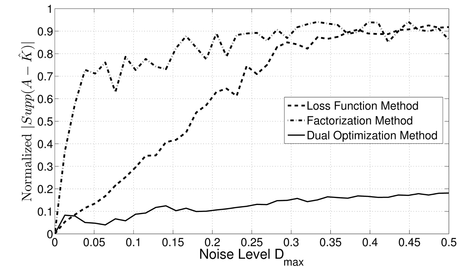


4.5 Numerical Comparison
We compare the performance of these methods. For three ideal clusters of size with noise level , we run all three algorithms for iterations. We consider an initial step size for all methods, and, for the loss function method, we doubel every iterations. For the dual method, we update for times and run iterations of the factorization method for the max-norm sub-problem at each update. We report the sparsity of the solution as well as the -norm of the error for each algorithm in Fig 4. This result shows that there is a trade-off between sparsity and the error – the dual optimization method provides consistently a sparse solution, where, factorization and loss function methods provide small error. The sparsity of loss function method gets worse as the noise increases.
5 Tighter Relaxations
In this section, we improve our basic algorithm in two ways: first, we use a tighter relaxation for valid clustering constraint and second, we add a single-linkage step after we recovered the clustering matrix. Although max-norm is a tighter relaxation comparing to trace-norm, we would like to go further and introduce tighter relaxations. Figure 5 summarizes different possible relaxations based on max-norm. The arrows in this figure indicated the strict subset relations among these relaxations. The tightest relaxation we suggest is based on the intuition that a clustering matrix is symmetric and has a trivial factorization , where, is non-zero if node belongs to cluster . Next lemma formalizes this result.
Lemma 2.
All relaxation sets shown in Fig. 5 are convex and the strict subset relations hold.


This suggests using the tightest convex relaxation, that is constraining to such that there exists with (the set of matrices with a factorization is called the set of completely positive matrices and is convex [5]). We optimize over this relaxation by solving the following optimization problem over :
| (6) | ||||
and setting . Although the constraint on is convex, the optimization problem (6) is not convex in .
5.1 Single-linkage Post Processing
The matrix extracted from (6) might diverge from a valid clustering matrix in two ways: firstly, it might not have the structure of a valid clustering and secondly, even if it has the structure, the values might not be integer. We run SLINK on as a “rounding scheme” to fix both of the above problems. SLINK gives a sequence of clusterings . To pick the best clustering, we choose
| (7) |
The matrix can be viewed as a refined version of the affinity matrix and hence the second step of the algorithm can be replaced by other hierarchical clustering algorithms. The criterion of choosing the best clustering in the hierarchy comes naturally from the correlation clustering formulation.
5.2 Comparison with Other Algorithms
We compare our enhanced algorithm with the trace-norm algorithm [16] followed by SLINK and SLINK itself. In all cases we pick a clustering from SLINK hierarchy using (7). The setup is identical to the experiment explained in Section 3.3. Fig 3 summarizes the results and shows that our enhanced algorithm outperforms all competitive methods significantly.
Besides the exact recovery of the underlying clustering, we would like to investigate that as noise level increases, how bad the output of our algorithm get. Using “variation of information” [23] as a distance measure for clusterings, we compare our algorithm with linear objective with trace-norm counterpart, SLINK and spectral clustering[32] for both balanced and unbalanced clusterings described before. For the spectral clustering method, we first find the largest principal components of and then, run SLINK on principal components. Fig 6(b) shows the result indicating that max-norm, even when the noise level is high and no method can recover the exact clustering, outputs a clustering that is not far from the true underlying clustering in our metric.
5.3 MNIST Dataset
To demonstrate our method in a realistic and larger scale data set, we run our enhanced algorithm, trace-norm and spectral clustering on MNIST Dataset [19]. For each experiment, we pick a total of data points from different classes ( from each class) and construct the affinities using Gaussian kernel as explained in [6]. We report the time complexities and clustering errors as previous experiment in Fig 7(b). For the spectral clustering, we take SVD using Matlab and pick the top 10 principal components followed by -means.
References
- [1] Ailon, N., Avigdor-Elgrabli, N., and Liberty, E. (2011). An improved algorithm for bipartite correlation clustering. European Symposium on Algorithms.
- [2] Alon, N. and Noar, A. (2006). Approximating the cut-norm via grothendieck’s inequality. SIAM Journal on Computing, 35.
- [3] Bagon, S. and Galun, M. (2011). Large scale correlation clustering optimization. Arxiv preprint arXiv:1112.2903.
- [4] Bansal, N., Blum, A., and Chawla, S. (2002). Correlation clustering. In Proceedings of the 43rd Symposium on Foundations of Computer Science.
- [5] Berman, A. and Shaked-Monderer, N. (2003). Completely Positive Matrices. World Scientific Publication.
- [6] Bühler, T. and Hein, M. (2009). Spectral clustering based on the graph p-laplacian. In Proceedings of the 26th Annual International Conference on Machine Learning, pages 81–88. ACM.
- [7] Burer, S. and Choi, C. (2006). Computational enhancements in low-rank semidefinite programming. Optimization Methods and Software, 21, 493–512.
- [8] Candes, E. J., Li, X., Ma, Y., and Wright, J. (2011). Robust principal component analysis? Journal of ACM, 58, 1–37.
- [9] Chan, P., Schlag, M., and Zien, J. (1994). Spectral k-way ratio cut partitioning. IEEE Trans. CAD-Integrated Circuits and Systems, 13, 1088–1096.
- [10] Chandrasekaran, V., Parrilo, P. A., and Willsky, A. S. (2010). Latent variable graphical model selection via convex optimization. arXiv:1008.1290.
- [11] Defays, D. (1977). An efficient algorithm for a complete link method. The Computer Journal (British Computer Society), 20, 364–366.
- [12] Dhillon, I., Guan, Y., and Kulis, B. (2005). A unified view of kernel k-means, spectral clustering and graph cuts. UTCS Technical Report TR-04-25, University of Texas at Austin.
- [13] Goemans, M. and Williamson, D. (1995). Improved approximation algorithms for maximum cut and satisfiability problems using semidefinite programming. Journal of ACM, 42.
- [14] Gray, L. and Wilson, D. (1980). Nonnegative factorization of positive semidefinite nonnegative matrices. Linear Algebra and its Applications, 31, 119–127.
- [15] Jain, A. K. and Dubes, R. C. (1981). Algorithms for Clustering Data. Prentice-Hall.
- [16] Jalali, A., Chen, Y., Sanghavi, S., and Xu, H. (2011). Clustering partially observed graphs via convex optimization. In ICML.
- [17] J.B., H.-U. and C., L. (1991). Convex Analysis and Minimization Algorithms I. Springer-Verlag, Netherland.
- [18] Langford, J., Li, L., and Zhang, T. (2009). Sparse online learning via truncated gradient. The Journal of Machine Learning Research, 10, 777–801.
- [19] LeCun, Y., Bottou, L., Bengio, Y., and Haffner, P. (1998). Gradient-based learning applied to document recognition. Proceedings of the IEEE, 86(11), 2278–2324.
- [20] Lee, J., Recht, B., Salakhutdinov, R., Srebro, N., and Tropp, J. (2010). Practical large-scale optimization for max-norm regularization. In NIPS.
- [21] Lee, T., Shraibman, A., and Spalek, R. (2008). A direct product theorem for discrepancy. In Proceedings of the IEEE 23rd Annual Conference on Computational Complexity.
- [22] Mathieu, C. and Schudy, W. (2010). Correlation clustering with noisy input. In Proceedings of the Twenty-First Annual ACM-SIAM Symposium on Discrete Algorithms, pages 712–728. Society for Industrial and Applied Mathematics.
- [23] Meilǎ, M. (2007). Comparing clusterings—an information based distance. Journal of Multivariate Analysis, 98, 873–895.
- [24] Meilǎ, M. and Shi, J. (2001). Learning segmentation by random walks. In NIPS.
- [25] Rockafellar, R. T. (1970). Convex Analysis. Prenticeton University Press; Princeton, NJ.
- [26] Shi, J. and Malik, J. (2000). Normalized cuts and image segmentation. IEEE Trans. Pattern Analysis and Machine Intelligence, 22(8), 888–905.
- [27] Sibson, R. (1973). Slink: an optimally efficient algorithm for the single-link cluster method. The Computer Journal (British Computer Society), 16(1), 30–34.
- [28] Sneath, P. M. A. and Sokal, R. R. (1973). Numerical Taxonomy. Freeman, San Francisco CA.
- [29] Srebro, N. (2004). Learning with Matrix Factorizations. Ph.D. thesis, Massachusetts Institute of Technology, Boston, MA.
- [30] Srebro, N., Rennie, J., and Jaakkola, T. (2005). Maximum-margin matrix factorization. In NIPS.
- [31] Steinhaus, H. (1957). Sur la division des corps matériels en parties. Bulletin de l’Acadbmie Polonaise des Sciences, 4, 801–804.
- [32] von Luxburg, U. (2007). A tutorial on spectral clustering. Statistics and Computing, Springer, 17.
- [33] Xu, H., Caramanis, C., and Sanghavi, S. (2012). Robust pca via outlier pursuit. IEEE Transactions on Information Theory.
- [34] Yu, S. X. and Shi, J. (2003). Multiclass spectral clustering. In International Conference on Computer Vision Proceedings.
Appendix A Proof of Lemma 2
Provided equivalences (1) and (2), it is clear that and are both convex sets. Since is the intersection of two sets and , it suffices to show that is a convex set. The set is called the set of completely positive matrices and has been shown to be a closed convex cone (see Theorem 2.2 in [5] for details).
For the proof of equivalence (1) see Lemma 15 in [29]. To prove equivalence (2), it is clear that . Now, suppose ; let and in contrary, assume that . This implies that at least one element on the diagonal of exceeds and hence . This is a contradiction and hence the equivalence (2) follows.
To show the relation (3), it suffices to show that the sub-set relation is strict, since the sub-set relation itself is trivial. By counter-example provided in [14], the sub-set relation is strict (i.e., there is a positive semi-definite and positive entry that does not belong to ).
Appendix B Proof of Lemma 1


We construct an example with that cannot be recovered. Consider the clustering shown in Fig. 8(a). It is clear that for this clustering, we have and
Now, consider the alternative clustering shown in Fig. 8(b). For this alternative clustering, we have
It is clear that (the alternative is a better clustering) for .
Appendix C Proof of Theorem 1
The proof has two main steps; in the first step, we characterize a sufficient optimality condition set based on the existence of a dual variable and in the second step, we construct such dual variable. For the sake of the proof, we consider a useful equivalent definition [21] of the max norm as
| (8) |
where, is the spectral norm (maximum eigenvalue) of the matrix and “” is the Hadamard element-wise product.
C.1 Notation
In this section, we introduce our notation and definitions used throughout the paper.
C.1.1 Residual Matrix Notations
In general, we do not expect the residual matrix to be sparse unless we threshold the affinity matrix (or we have adjacency matrix). However, to provide a guarantee, we need to characterize the sub-gradient of the -norm and hence distinguish between zeros and non-zeros of . Let
| (9) |
where, is the index set of non-zero entries. The orthogonal projection of a matrix to this space is defined to be a matrix of the same size with if and zero otherwise. The orthogonal complement of this space is denoted by and the projection is defined as .
C.1.2 Clustering Matrix Notations
Let be constructed as
| (10) |
Define to be the space of matrices sharing either row or column space with . The orthogonal projection to this space can be defined as
where,
Denote the orthogonal complement of the space by equipped with projection . Let be the contraction between the ideal clusters and disagreements (See Lemma 5 for more details on this definition). Under the assumption of the theorem, we have and hence, .
Using definitions in (11), let
where,
Notice that and hence . If we show that has spectral norm less than , then it is immediate that . Also, we have an eigenvalue decomposition , where, is as defined above and contains the eigenvector(s) corresponding to the maximum magnitude eigenvalue (with repetitions). To bound the spectral norm of , consider
The first inequality follows from Lemma 6. We make assumptions so that the last inequality holds.
We use the variational form (8) to characterize the sub-gradient of the max-norm at the point .
Lemma 3.
For a matrix , we have if , for some diagonal positive semi-definite matrix with and for some matrix with and .
C.2 Sufficient Optimality Conditions
We provide similar optimality conditions to those provided in plus trace norm minimization in the literature. The main difference here is the existence of the auxiliary variable in the conditions. The following lemma characterizes a sufficient optimality condition set.
Lemma 4 (Sufficient Optimality Condition.).
Proof.
Notice that since by construction has no zero entry (except for the very corner case where there are only two clusters both of size ), the matrix can take any value/sign on each entry by choosing the values of properly. Under these conditions, and also and the result follows from the standard first order optimality argument and zero duality gap of both and max norms.
∎
C.3 Dual Variable Construction
First notice that under the assumption of the theorem, we have and hence, by Lemma 5, we have and also is feasible. Second, we construct by using alternating projections. Consider the infinite sums
| (11) | ||||
By the proof of the Lemma 5, these sums converge geometrically with parameter (See Lemma 5 in [16] for the proof). Denoting element-wise division with “” (and ), let
It is easy to check that conditions (a) and (c) in lemma 4 are both satisfied for . To show condition (b), first notice that and hence, we have
The last inequality holds for . For the condition (d), we have
The last inequality holds for as assumed.
Lemma 5.
If then .
Proof.
We show that the projection has a norm strictly less than one. Then, if there exists a non-zero matrix , then is a trivial contradiction. Let and consider
The last step is attained by optimizing over and . This concludes the proof of the lemma.
∎
Lemma 6.
.
Proof.
For , we have , where, with . By definition of , we have . Thus,
The rest of the proof is straight forward as follows
This concludes the proof of the lemma.
∎