Locality in Theory Space

We define a local $N$-site cyclic moose with gauge group $\mathrm{SU}(n)$ by the Lagrangian

as shown in Figure 1. The $\mathfrak{su}(n)$-valued field strengths $F^{i}_{\mu\nu}(x)$ live on the sites $i=1,2,\dots,N$, and the link fields $\Sigma_{j}\in\mathrm{SU}(n)$ live on the links between sites $j$ and $j+1$.²² 2 For ease of notation, we freely raise and lower site indices on gauge and link fields. There is a periodic identification of sites and links by $i\simeq i+N$. The sites are shaded to represent gauge symmetries, as opposed to global symmetries which will be important in our discussion of the QCD moose in Section 6.1.

Our normalization for the $\mathfrak{su}(n)$ generators $T^{a}$ is

The gauge transformations of the link fields are

where $U_{j},U_{j+1}\in\mathrm{SU}(n)$ are in the fundamental representation, so $\Sigma_{j}$ transforms in the antifundamental $\overline{\mathbf{n}}$ of the site to its left and the fundamental $\mathbf{n}$ of the site to its right. This behavior is represented by the directional arrows on the link fields in Figure 1. The covariant derivative is defined by

where we use canonical normalization for the gauge fields so the gauge couplings $g_{j}$ appear explicitly.

Writing

the Lagrangian (3) becomes a nonlinear sigma model in 3+1 dimensions describing the interactions of the “pions” $\pi_{j}$ with themselves and the gauge fields $A^{i}_{\mu}$. Pursuing this analogy with low-energy QCD, we refer to $f_{j}$ as decay constants. With the normalization convention (4), we obtain canonically normalized kinetic terms for the $\pi$ fields after expanding the Lagrangian as a power series in the $\pi_{j}^{a}$. The remainder of the Lagrangian involving $\pi_{j}^{a}$ consists of derivative interactions suppressed by powers of $1/f_{j}$, all of which are nonrenormalizable operators. Thus, the nonlinear sigma model has some UV cutoff, which we will take to be the scale of tree-level unitarity violation $\Lambda$; we will define $\Lambda$ precisely in Section 4.1. Keeping only the leading terms with coefficients $1/f_{j}^{2}$, one can estimate the scale of unitarity violation by “naive dimensional analysis” [21],

Note that $\Lambda$ is determined by the minimum of the $f_{j}$ because $\pi_{i}$ and $\pi_{j}$ are decoupled for $i\neq j$, so each link has its own scale of unitarity violation, and unitarity violation for the whole moose is dominated by whichever one occurs first.

With the parameterization (7), each $\Sigma_{j}$ gets a vacuum expectation value (vev) $\langle\Sigma_{j}\rangle=\mathds{1}$ and the link fields spontaneously break the gauge symmetry at each site, with $\pi_{j}$ acting as Goldstone bosons which are eaten by the gauge fields $A^{j}_{\mu}$. The remaining unbroken gauge symmetry is the diagonal $\mathrm{SU}(n)$ subgroup, whose gauge coupling $g_{4}$ (in a notation suggestive of KK decomposition) is given by

Since this is a cyclic moose, there is also an uneaten linear combination of Goldstone modes $\tilde{\pi}=(\pi_{1}+\pi_{2}+\cdots+\pi_{N})/\sqrt{N}$, which we will sometimes refer to as the winding mode.

The mass-squared matrix for the now-massive gauge fields arises from the second term in Eq. (3) by setting $\Sigma_{j}=\langle\Sigma_{j}\rangle=\mathds{1}$. Setting the gauge couplings to a common value $g$,

This matrix has a zero eigenvalue for all choices of $f_{j}$, with eigenvector $A^{(0)}=(A_{1}+A_{2}+\cdots+A_{N})/\sqrt{N}$, corresponding to the diagonal subgroup mentioned above. If we further restrict the decay constants $f_{j}$ to be equal ($f_{j}\equiv f$), we have an analytic expression for the mass spectrum of the cyclic moose:

With the exception of Section 6.2 where we explore warped spaces, we will always set the decay constants and gauge couplings equal, $f_{j}\equiv f$ and $g_{i}\equiv g$, corresponding to a discrete translation invariance along the moose.

The Lagrangian (3) can be interpreted as a (4+1)-dimensional lattice gauge theory where only the compact fifth dimension has been latticized, with the $\Sigma_{j}$ providing the fifth component of the five-dimensional gauge field in the continuum limit where the lattice spacing goes to zero. The continuum limit is ordinary five-dimensional Yang-Mills

where $M,N=0,1,2,3,5$ and

Using this interpretation, known as dimensional deconstruction, we obtain a dictionary between parameters in the Lagrangian and parameters in the latticized theory [1]:

The last of these relations identifies the gauge coupling of the diagonal subgroup ($g_{4}$ in Eq. (9)) with the the effective four-dimensional gauge coupling of the KK zero mode of the five-dimensional theory after compactification.

The five-dimensional interpretation of the deconstruction can be confirmed in several ways. First, the dictionary preserves the usual relation between four- and five-dimensional gauge couplings after compactification:

Second, we can examine the mass spectrum of Eq. (11) in the continuum limit, $N\to\infty$ and $a\to 0$ with $R$ fixed:

for small integers $|k|$. This is precisely the KK spectrum of modes on a circle of circumference $R$, as one would expect from compactification of a fifth dimension. In this picture, the uneaten linear combination of Goldstone bosons corresponds to the nontrivial Wilson loop around the compact extra dimension, hence the name “winding mode” for $\tilde{\pi}$.

In the framework of dimensional deconstruction, locality in the latticized dimension is built into Eq. (3) through locality in theory space. Indeed, the field strengths $F^{i}_{\mu\nu}$ are decoupled at different sites $i\neq j$, and the $\Sigma_{j}$ only couple to nearest-neighbor gauge fields $A^{j}_{\mu}$ and $A^{j+1}_{\mu}$ through Eq. (6). In the continuum limit, $D_{\mu}\Sigma_{j}$ becomes a covariant derivative along the latticed direction, which is also local. In the original application of dimensional deconstruction, derived these local interactions by starting with a moose with additional fermions charged under a “color” gauge group, which confines to give the $\Sigma$ fields as fermion bilinears. However, in our analysis we take Eq. (3) as our starting point, with the $\Sigma_{j}$ as “fundamental” fields rather than composite operators.

The aim of this paper is to study nonlocality in theory space, which we will incorporate by perturbing the local moose (3) by a gauge-invariant operator $\epsilon f^{2}\mathcal{O}$, where $\epsilon$ is small and dimensionless and $f^{2}$ is inserted for normalization.³³ 3 While the squares of the decay constants $f_{j}^{2}$ must be positive for the $\pi_{j}$ kinetic terms to have the correct sign, there is no such restriction on the sign of $\epsilon$, although $\epsilon$ must be real. For $\mathcal{O}$ to be nonlocal, it must connect distant sites $i$ and $j$, and hence transform in the $\overline{\mathbf{n}}$ of $\mathrm{SU}(n)_{i}$ and the $\mathbf{n}$ of $\mathrm{SU}(n)_{j}$. We could simply define a new link field $\widetilde{\Sigma}$ connecting these sites, but we are interested in comparing theories with the same number of four-dimensional degrees of freedom. Moreover, the theory with this extra field has a pathological local limit, since as its decay constant $\tilde{f}$ goes to zero, $\widetilde{\Sigma}$ disappears but unitarity is violated immediately due to Eq. (8).⁴⁴ 4 Even if fields like $\widetilde{\Sigma}$ were present in the original Lagrangian, we could always decouple them with the plaquette operator $\mu^{2}f^{2}\,\mathrm{Tr}\,|\Sigma_{i}\Sigma_{i+1}\cdots\Sigma_{j}\widetilde{\Sigma}^{\dagger}|^{2}$. As we take $\mu\to\infty$, $\widetilde{\Sigma}$ becomes massive and decouples from the low-energy spectrum.

Instead, we choose to consider

for $i<j$, and we will refer to this as a “hopping” term with $N_{\text{hop}}=j-i$.⁵⁵ 5 The factor of 2 is purely conventional and simplifies some formulas in what follows. To preserve the discrete translation invariance in the compact dimension, we sum over all sites:

Figure 2 shows an example of a 6-site moose diagram with such nonlocal terms for both $N_{\text{hop}}=1$ and $N_{\text{hop}}=2$. The goal of Section 5 will be to study the effect of $\mathcal{O}_{N_{\text{hop}}}$ on the cutoff scale $\Lambda$. For simplicity, we will only consider perturbing the local moose by a nonlocal term with a single value of $N_{\text{hop}}$ (unlike in Figure 2) so that we can study the effect of nonlocality as a function of the nonlocal length scale. We will abbreviate $\mathcal{O}_{N_{\text{hop}}}\equiv\mathcal{O}_{\text{NL}}$ and display all results as a function of $N_{\text{hop}}$.

To construct the continuum version of this operator, we define the characteristic nonlocal length scale $\ell$ by

The deconstructed fields $\Sigma$ and $A_{\mu}$ are related to the continuum five-dimensional gauge field $\widehat{A}_{M}$ by

where $y$ is the coordinate along the fifth dimension and $P$ is the path-ordering symbol. These relations imply that in the continuum limit,

so our nonlocal operator is a nonlocal gauge kinetic term, connecting $\widehat{F}_{\mu 5}(x,y)$ and $\widehat{F}^{\mu 5}(x,y+\ell)$ by means of a Wilson line along the fifth dimension,

In the five-dimensional picture, Eq. (20) is the natural nonlocal operator to consider, as compared to operators like $|D_{\mu}(\Sigma_{i}\,\Sigma_{i+1}\,\cdots\Sigma_{j})|^{2}$. The continuum analogue of the latter is $|D_{\mu}W(y,y+\ell)|^{2}$, which does not have any simple interpretation. Moreover, such an operator is redundant, because

so this operator already contains kinetic terms for $\Sigma_{i}$ through $\Sigma_{j}$.⁶⁶ 6 This redundant nonlocal operator will appear in the three-site QCD moose in Section 6.1, and in the discussion of KK matching in Appendix A.3. As a result, to lowest order in $\epsilon$ the effect of $\epsilon|D_{\mu}(\Sigma_{i}\,\Sigma_{i+1}\,\cdots\Sigma_{j})|^{2}$ would be to simply shift the decay constant $f^{2}\to f^{2}(1+\epsilon)$, a trivial change which can be absorbed by a redefinition of the $\pi_{i}$. In addition, after subtracting off the kinetic terms from $\epsilon|D_{\mu}(\Sigma_{i}\,\Sigma_{i+1}\,\cdots\Sigma_{j})|^{2}$, we are left precisely with terms like $\mathcal{O}_{N_{\text{hop}}}^{(i)}$, but for all values of $N_{\text{hop}}\leq|j-i|$. To isolate a single nonlocal length scale $\ell$, we will only consider the nonlocal operator (21).

We are always free to add additional terms (local or nonlocal) which have more than two derivatives, as long as they respect the symmetries present in the original local Lagrangian. However, in a momentum power-counting scheme, it is consistent to truncate the effective Lagrangian to order $p^{2}$ provided we restrict the analysis to tree-level, as we will do in this paper. Indeed, two derivatives are the minimum required to have any nontrivial nonlocal interaction, and these nonlocal terms in Eq. (21) are the same order in momentum as the nonlinear sigma model kinetic terms $|D_{\mu}\Sigma|^{2}$ appearing in the local Lagrangian. If we wanted to study the effects of higher-derivative terms, then by Weinberg’s power-counting theorem [22], we would also have to consider one-loop amplitudes of two-derivative terms. Such effects are certainly important, but we leave an analysis to order $p^{4}$ to future work.⁷⁷ 7 This power-counting also explains why we do not consider nonlocal terms like $\mathrm{Tr}\,(F_{\mu\nu}\,\Sigma\,F^{\mu\nu}\,\Sigma^{\dagger})$; as is well-known from chiral perturbation theory, these terms count as $p^{4}$ in momentum.

The leading unitarity-violating pieces of massive gauge boson scattering amplitudes arise from the scattering of longitudinal polarization states. In the limit of high-energy scattering, for sufficiently small values of the gauge coupling $g$, the Goldstone equivalence theorem [23, 24] allows us to replace longitudinally-polarized gauge bosons by the corresponding (eaten) Goldstone modes when computing amplitudes.

Because the scattering amplitudes depend nontrivially on the gauge indices, computing the scale of unitarity violation for a given scattering channel $\pi^{a}\pi^{b}\to\pi^{c}\pi^{d}$ does not give the full information about the scale of unitarity violation for the whole collection of Goldstone modes. Instead, we use a coupled-channel analysis [25] where we compute the whole scattering matrix $\mathcal{T}^{abcd}$ and define the scale of unitarity violation using its largest eigenvalue $\lambda_{\rm max}$.

The conventional normalization of the scattering matrix for partial waves labeled by $J=0,1,\dots$ is (following the notation of ),

where $\langle\alpha|\mathcal{T}|\beta\rangle$ is the scattering amplitude between properly normalized in and out states $|\alpha\rangle$ and $|\beta\rangle$, and $P_{J}(\cos\theta)$ is the $J$-th Legendre polynomial. As in earlier applications of this coupled-channel analysis [25, 26, 27, 18], the $J=0$ $s$-wave piece provides the strictest bounds. Expressing the amplitudes in terms of the Mandelstam variables $s$, $t=-\frac{s}{2}(1+\cos\theta)$, and $u=-\frac{s}{2}(1-\cos\theta)$, the integration in Eq. (32) for $J=0$ amounts to the replacement $t,u\to-s/2$ in the amplitude $\mathcal{T}$ and simply contributes a factor of 2 from $d\cos\theta$.

For unitarity to hold, the largest eigenvalue of the $s$-wave partial amplitude must satisfy¹²¹² 12 The precise numerical value of the unitarity bound is not important for our analysis. If we wished, we could use this freedom to suppress the effects of unknown four-derivative terms, whose amplitudes grow as $p^{4}$. For example, imposing $|\text{Re}\,(a^{(0)})|<1/4$ (corresponding to the scale of “half-unitarity violation”) would suppress such terms by a factor of $(1/2)^{2}=1/4$. In our analysis, all that matters is the parametric dependence of $\Lambda_{\rm NL}/\Lambda_{\rm local}$ on $\epsilon$, which is unchanged by such manipulations. $|\text{Re}\,(a^{(0)})|<1/2$, leading to the condition on the amplitude¹³¹³ 13 Note that $\lambda(s)$ will be real for the tree-level amplitudes we consider in this paper, so $|\lambda(s)|$ is an absolute value and not a complex modulus.

where $\lambda(s)$ is the largest eigenvalue of the $\mathcal{T}$ matrix expressed as a function of the Mandelstam variable $s$ (after the replacement $t,u\to-s/2$). For the Goldstone equivalence limit we consider in this paper, the eigenvalues will be linear in $s$, so we can define $\lambda^{\prime}\equiv\partial\lambda/\partial s$. By solving for $\sqrt{s}$, we obtain the scale of unitarity violation:

Since the $\mathcal{T}$ matrix (expressed as a function of $s$) is related to the $s$-wave piece $a^{(0)}$ by numerical factors, we can work directly with $\mathcal{T}$ and get the scale of unitarity violation from Eq. (34).

To compute the gauge boson scattering matrix for the local moose in the high-energy limit, we can derive Feynman rules directly from the $|D_{\mu}\Sigma_{j}|^{2}$ part of the Lagrangian, expressed in terms of the Goldstone fields $\pi^{a}_{j}$. Because we work in the high-energy limit, we need not work in the basis of Goldstones which are eaten by the gauge boson mass eigenstates; rather, we work in a basis which makes the global symmetries of the scattering matrix manifest.¹⁴¹⁴ 14 In fact, computed all amplitudes in the mass eigenstate basis, but found that only a coupled-channel analysis reproduced the correct unitarity behavior. The dominant channel is precisely the one we find in the Goldstone basis.

The $\pi_{j}\to-\pi_{j}$ reflection symmetry of the Lagrangian (3) implies the absence of terms odd in $\pi_{j}$, and hence the leading-order interaction is a 4-point term,

The Feynman diagram contributing to $\pi\pi\rightarrow\pi\pi$ scattering is shown in Figure 3. Notice that for the local Lagrangian, $\pi_{i}$ and $\pi_{j}$ are totally decoupled for $i\neq j$.

Now, consider the $\mathcal{T}$ matrix for an SU(2) moose, which will be our starting point for introducing nonlocality in the following section. Because all of the $N$ link fields are decoupled, $\mathcal{T}$ consists of $N$ copies of the $\mathcal{T}$ matrix for one link, allowing us to drop link indices in what follows. The Goldstone modes are triplets of $\mathrm{SU}(2)$, so the two-particle scattering states decompose into irreducible representations of $\mathrm{SU}(2)$ as $\mathbf{3}\otimes\mathbf{3}=\mathbf{1}\oplus\mathbf{3}\oplus\mathbf{5}$. Borrowing the language of chiral perturbation theory, the pions $\pi^{a}$ are in the isospin $I=1$ representation, and scattering takes place between two-particle states of definite total isospin $I=0,1,2$.

By Bose symmetry, the $s$-wave scattering amplitude vanishes for the antisymmetric $I=1$ states. The remaining nonzero eigenvalues can be calculated analytically by diagonalizing $\mathcal{T}$:

so the largest eigenvalue (strictly speaking, the eigenvalue of largest magnitude) is in the $I=0$ sector. We will refer to the corresponding eigenvector as the gauge singlet state¹⁵¹⁵ 15 The additional normalization factor of $1/\sqrt{2}$ accounts for the fact that in the isospin basis, the final state particles for each isospin channel are identical.

As we will see, the fact that the gauge singlet is associated with the largest eigenvalue is the key property which implies the vanishing of the leading-order nonlocal contribution to the scattering matrix. Using $\lambda_{\rm max}\equiv\lambda_{I=0}$ in Eq. (34) gives a scale of unitarity violation

Note that this is stronger than the naive dimensional analysis bound (8) by a factor¹⁶¹⁶ 16 This leads to a very rough estimate of the effects of four-derivative terms at the cutoff. The NDA bound is the scale at which one-loop effects are comparable to tree-level effects, so at the actual cutoff, one can estimate the size of tree-level four-derivative terms as being suppressed relative to the local two-derivative terms by a factor of $(\Lambda_{\rm local}/\Lambda_{\rm NDA})^{2}\approx 1.6$. of $\sqrt{\pi/2}\approx 1.25$. Furthermore, the largest amplitude for any individual scattering channel $\pi^{a}\pi^{a}\to\pi^{b}\pi^{b}$ is a factor of 2 smaller than that of the gauge singlet; performing the coupled-channel analysis strengthens the unitarity bounds considerably. Including the results for $\overline{m}_{\rm local}$ from Eq. (30), the normalized ratio $\mathcal{R}$ for the local theory is

The effect of the nonlocal term (21) on the spin-1 mass matrix is straightforward. Any individual hopping term $\mathcal{O}_{N_{\text{hop}}}^{(i)}$ contains new covariant derivatives $D_{\mu}\Sigma_{i}$ and $D^{\mu}\Sigma_{i+N_{\text{hop}}}$. After setting $\Sigma_{i}$ to its vev $\langle\Sigma_{i}\rangle=\mathds{1}$, the contribution of $\mathcal{O}_{N_{\text{hop}}}^{(i)}$ to the mass matrix is

where the upper-left corners of the $2\times 2$ blocks are inserted at the positions $(i,i+N_{\text{hop}})$ and $(i+N_{\text{hop}},i)$. Unless $N_{\text{hop}}$ is equal to 0 or $\pm 1$ modulo $N$, the perturbation does not affect the diagonal elements, and hence $\mathrm{Tr}\,M^{2}$ is unchanged. Thus, the scale $\overline{m}$ is identical to the local case, as long as $1<N_{\text{hop}}<N-1$:

As desired from Section 3, $\overline{m}$ is insensitive to the nonlocal perturbation, allowing $\mathcal{R}$ to depend on nonlocality only through $\Lambda$. The case $N_{\text{hop}}\equiv\pm 1$ (mod $N$) can be considered as a discretization error arising from the fact that an $N$-site moose for finite $N$ has a minimum nonlocal length scale $\ell=a$, where $a$ is the lattice spacing.

In general, numerical methods are needed to compute the exact eigenvalues of the scattering matrix as a function of the nonlocal coefficient $\epsilon$. Here, we will resort to perturbation theory in $\epsilon$, considering the effect of small nonlocal terms. By ‘‘perturbation theory,’’ we mean finding the largest eigenvalue of the scattering matrix, using techniques familiar from nonrelativistic quantum mechanics.¹⁸¹⁸ 18 Of course, throughout this paper we are using ordinary perturbation theory appropriate to quantum field theory to compute scattering amplitudes from tree-level Feynman diagrams. Taking the finite-dimensional $\mathcal{T}$ matrix as our “Hamiltonian,” we can calculate the scattering matrix eigenvalues order-by-order in $\epsilon$ in terms of the unperturbed scattering eigenstates from the local Lagrangian.

As we will see below, the nonlocal terms change the kinetic matrix for the $\pi$ fields, requiring field redefinitions to compute scattering between canonically normalized states. Before the field redefinitions, only the nonlocal terms carry factors of $\epsilon$, but expanding the field redefinition matrix as a series in $\epsilon$, both the local and nonlocal terms can contribute to tree-level scattering amplitudes at all orders in $\epsilon$. To keep track of $\epsilon$ in the total amplitude, we have to apply perturbation theory to the somewhat unusual case of a matrix perturbed by contributions to all orders in $\epsilon$. To second order in $\epsilon$, the scattering matrix $\mathcal{T}$ and its largest eigenvalue $\lambda$ are

The fact that the nonlocal term still preserves the cyclic symmetry determines the structure of the eigensystem of the scattering matrix. Indeed, the eigenstates of the full scattering matrix must respect the cyclic symmetry, and in particular there is no mixing of states with different eigenvalues under the operator which implements translations from site $i$ to $i+1$. Thus we can work in the subspace of cyclically-invariant states with eigenvalue zero under this operator. An orthonormal basis of two-particle $\mathrm{SU}(2)$ singlet states $|q\rangle$ spanning this subspace is

For instance, in this notation we have

where $|S_{i}\rangle$ are the gauge singlet states introduced in Eq. (37), now with a link index. In the local theory, all of the $\mathrm{SU}(2)$ singlets $|S_{i}\rangle$ are degenerate with eigenvalue

so this is also the eigenvalue of $|0\rangle$. By the arguments above, the eigenstate of the nonlocal theory with the largest eigenvalue must contain $|0\rangle$, plus order $\epsilon$ contributions from $|q\rangle$:

With the correct basis in hand, the lowest-order contribution to $\lambda$ at first order in $\epsilon$ is

However, as we show in Section 5.4, this contribution vanishes identically for $N_{\text{hop}}<N$, due to a trace-related cancellation peculiar to the gauge structure of the singlet state and not because of any symmetry argument one can make at the Lagrangian level. Indeed, first-order shifts are generic for the other eigenvalues belonging to the $\bm{3}$ and $\bm{5}$ components of $\mathcal{T}$, and as we will see the vanishing of the shift for the singlet requires a detailed look at the structure of the relevant Feynman rules. The fact that the singlet state is associated with the largest eigenvalue is a necessary condition for locality to maximize $\Lambda$; otherwise, $\Lambda_{\rm NL}$ could be larger or smaller than $\Lambda_{\rm local}$ depending on the sign of $\epsilon$.

Because of the first-order cancellation, we must go to second order in $\epsilon$. The first-order eigenvector coefficients for Eq. (47) are

which is the usual formula from ordinary perturbation theory. Note that the usual energy denominator $\lambda^{(0)}-\lambda_{q}^{(0)}$ is replaced by just $\lambda^{(0)}$ because the $|q\rangle$ states for $q\neq 0$ have zero eigenvalues in the unperturbed $\mathcal{T}$ matrix. The second-order eigenvalue shift $\lambda^{(2)}$ is

which is the usual formula plus an extra term $\langle 0|\mathcal{T}_{2}|0\rangle$, which in this context contains contributions from both the local and nonlocal terms. As we will see below, the contribution from the eigenstates $|q\rangle$ is essential, giving the leading behavior in $N_{\text{hop}}$ and illustrating once again the necessity of doing a coupled-channel analysis rather than focusing on single scattering channels.

The nonlocal term (21) has several interesting effects on the scattering matrix and, by extension, on the scale of unitarity violation $\Lambda_{\text{NL}}$:

• •

  $\mathcal{O}_{\text{NL}}$ breaks the reflection symmetry $\pi_{j}\to-\pi_{j}$, so 3-point terms are present, unlike in the local Lagrangian.

• •

  Despite only transforming under the gauge symmetries corresponding to sites $i$ and $i+N_{\text{hop}}$, the operator $\mathcal{O}^{(i)}_{N_{\text{hop}}}$ contains all the link fields between sites $i$ and $i+N_{\text{hop}}$, and hence several new intermediate states in 3-point diagrams are available to contribute to the gauge singlet scattering channel. These will cause the matrix elements $\langle 0|\mathcal{T}_{2}|0\rangle$ to scale like $N_{\text{hop}}$, though $\langle 0|\mathcal{T}_{1}|q\rangle\sim N_{\text{hop}}$ will turn out to give the dominant contribution to $\lambda^{(2)}$.

• •

  As mentioned above, since $\mathcal{O}_{\text{NL}}$ contains $\partial_{\mu}\pi$ terms, it changes the kinetic matrix of the $\pi$ fields. One must perform a field redefinition in order to recover canonical kinetic terms corresponding to the physical fields which participate in scattering.

Before the necessary field redefinitions, the operators present in the Lagrangian are as follows, writing $i^{\prime}$ for $i+N_{\text{hop}}$ for ease of notation:

• •

  Local 4-point terms, independent of $\epsilon$:

• •

  Nonlocal 3-point terms, proportional to $\epsilon$:

• •

  Nonlocal 4-point terms, proportional to $\epsilon$:¹⁹¹⁹ 19 We have abbreviated the third line because it does not contribute to any relevant amplitudes in our calculation. The omitted terms simply involve various permutations of the group and site indices.

Lorentz indices are suppressed everywhere since the Lorentz structure of all terms is identical, summation over the group indices $a,b,c,d$ is assumed, and the group theory factors for $\mathrm{SU}(2)$ are ($a,b,c,d=1,2,3$)

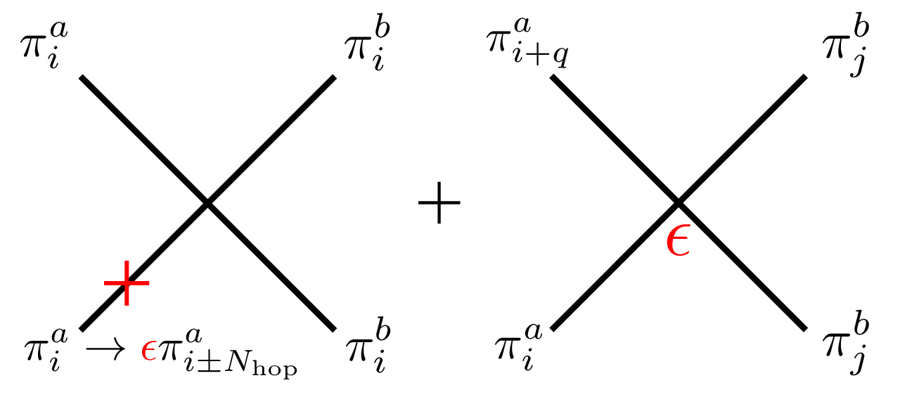
To take into account the field redefinition, we show in Appendix B.1 that to order $\epsilon^{2}$, the wavefunction factor $Z^{-1/2}_{ij}$ is

Note in particular that the diagonal elements $Z^{-1/2}_{ii}$ have no order-$\epsilon$ components. After the field redefinitions, we have the following contributions to the gauge singlet piece of the scattering matrix:

• •

  Order $\epsilon^{0}$: local 4-point diagrams only, with no field redefinitions (Figure 3). These contribute only to $\lambda^{(0)}$.

• •

  Order $\epsilon$: local 4-point diagrams with order-$\epsilon$ field redefinitions and nonlocal 4-point diagrams with no field redefinitions (Figure 4). Since $\langle 0|\mathcal{T}_{1}|0\rangle$ vanishes, these only contribute to $\langle 0|\mathcal{T}_{1}|q\rangle$, which dominates $\lambda^{(2)}$.

• •

  Order $\epsilon^{2}$: local 4-point diagrams with order-$\epsilon^{2}$ field redefinitions and nonlocal 4-point diagrams with order-$\epsilon$ field redefinitions (Figure 5), diagrams with two nonlocal 3-point vertices and no field redefinitions (Figure 6). These contribute to $\langle 0|\mathcal{T}_{2}|0\rangle$, which give a subleading (in $N_{\text{hop}}$) correction to $\lambda^{(2)}$. Note that the first appearance of 3-point terms comes at order $\epsilon^{2}$.

We now have all of the ingredients to calculate $\lambda$ to order $\epsilon^{2}$. First, we can show that the first-order shift vanishes for the singlet state as long as $N_{\text{hop}}<N$. As mentioned above, we must consider the local terms with field redefinitions and the nonlocal terms separately. The local terms (35) are all even in $\pi_{i}$, and so after field redefinitions according to (54), the order-$\epsilon$ pieces are odd in $\pi_{i}$, and thus do not contribute to the matrix element $\langle 0|\mathcal{T}_{1}|0\rangle$ between singlet states. The relevant nonlocal terms in Eq. (52) would be of the form $\epsilon\partial\pi_{i}^{a}\pi_{i}^{a}\partial\pi_{i\pm N_{\text{hop}}}^{b}\pi_{i\pm N_{\text{hop}}}^{b}$ for fixed group indices $a$ and $b$, but these terms vanish identically due to cyclicity of the trace.²⁰²⁰ 20 This argument breaks down when $N_{\text{hop}}\geq N$, because $\mathcal{O}_{\text{NL}}$ contains the redundant kinetic terms discussed in Section 2.3, which add extra terms to the second line of Eq. (52) and destroy the trace-related cancellation. This gives a contribution to the scattering matrix which goes like $\epsilon k^{2}$, where $k$ is the “winding number” around the fifth dimension. The structure of the field redefinition matrix also changes for $N_{\text{hop}}=kN$, giving a further local contribution. This can be seen explicitly by setting the appropriate indices equal in the second line of Eq. (52) and using $\mathrm{Tr}\,(T^{a}(T^{b})^{2}T^{a})=\mathrm{Tr}\,((T^{a})^{2}(T^{b})^{2})$. So there are no contributions to order $\epsilon$ in the singlet channel:

This result depends only on the cyclicity of the trace and not on the particular form of the group theory factors (53), and holds for any gauge group such that the largest eigenvalue corresponds to the singlet state.²¹²¹ 21 This is the case for $\mathrm{SU}(n)$ and is expected to be true for other gauge groups [26]. In fact, the vanishing of the first-order singlet amplitude does not depend on the cyclic symmetry. The relevant nonlocal terms in Eq. (52) vanish for each individual hopping term $\mathcal{O}_{N_{\text{hop}}}^{(i)}$, and the field redefinitions do not contain any order-$\epsilon$ diagonal terms, as we show in Appendix B.1, thus ensuring that the local terms do not contribute either.

Calculating the second-order eigenvalue shift requires the matrix elements $\langle 0|\mathcal{T}_{1}|q\rangle$ and $\langle 0|\mathcal{T}_{2}|0\rangle$ in Eq. (50). The matrix elements $\langle 0|\mathcal{T}_{1}|q\rangle$ come from terms in the Lagrangian schematically of the form

References

- (1) N. Arkani-Hamed, A. G. Cohen, and H. Georgi, (De)constructing dimensions, Phys.Rev.Lett. 86 (2001) 4757–4761, [hep-th/0104005].
- (2) J. M. Maldacena, The Large N limit of superconformal field theories and supergravity, Adv.Theor.Math.Phys. 2 (1998) 231–252, [hep-th/9711200].
- (3) S. Gubser, I. R. Klebanov, and A. M. Polyakov, Gauge theory correlators from noncritical string theory, Phys.Lett. B428 (1998) 105–114, [hep-th/9802109].
- (4) E. Witten, Anti-de Sitter space and holography, Adv.Theor.Math.Phys. 2 (1998) 253–291, [hep-th/9802150].
- (5) I. Heemskerk, J. Penedones, J. Polchinski, and J. Sully, Holography from Conformal Field Theory, JHEP 0910 (2009) 079, [arXiv:0907.0151].
- (6) I. Heemskerk and J. Sully, More Holography from Conformal Field Theory, JHEP 1009 (2010) 099, [arXiv:1006.0976].
- (7) A. Fitzpatrick, E. Katz, D. Poland, and D. Simmons-Duffin, Effective Conformal Theory and the Flat-Space Limit of AdS, JHEP 1107 (2011) 023, [arXiv:1007.2412].
- (8) R. Sundrum, From Fixed Points to the Fifth Dimension, arXiv:1106.4501.
- (9) A. Fitzpatrick and J. Kaplan, Analyticity and the Holographic S-Matrix, arXiv:1111.6972.
- (10) R. Chivukula, D. A. Dicus, and H.-J. He, Unitarity of compactified five-dimensional Yang-Mills theory, Phys.Lett. B525 (2002) 175–182, [hep-ph/0111016].
- (11) R. S. Chivukula and H.-J. He, Unitarity of deconstructed five-dimensional Yang-Mills theory, Phys.Lett. B532 (2002) 121–128, [hep-ph/0201164].
- (12) S. De Curtis, D. Dominici, and J. R. Pelaez, Strong tree level unitarity violations in the extra dimensional standard model with scalars in the bulk, Phys.Rev. D67 (2003) 076010, [hep-ph/0301059].
- (13) M. D. Schwartz, Constructing gravitational dimensions, Phys.Rev. D68 (2003) 024029, [hep-th/0303114].
- (14) H. Georgi, Vector Realization of Chiral Symmetry, Nucl.Phys. B331 (1990) 311–330.
- (15) L. Randall and R. Sundrum, A Large mass hierarchy from a small extra dimension, Phys.Rev.Lett. 83 (1999) 3370–3373, [hep-ph/9905221].
- (16) L. Randall and R. Sundrum, An Alternative to compactification, Phys.Rev.Lett. 83 (1999) 4690–4693, [hep-th/9906064].
- (17) H. Abe, T. Kobayashi, N. Maru, and K. Yoshioka, Field localization in warped gauge theories, Phys.Rev. D67 (2003) 045019, [hep-ph/0205344].
- (18) R. Chivukula, E. H. Simmons, H.-J. He, M. Kurachi, and M. Tanabashi, Deconstruction and Elastic pi pi Scattering in Higgsless Models, Phys.Rev. D75 (2007) 035005, [hep-ph/0612070].
- (19) L. Randall, Y. Shadmi, and N. Weiner, Deconstruction and gauge theories in AdS(5), JHEP 0301 (2003) 055, [hep-th/0208120].
- (20) A. Falkowski and H. D. Kim, Running of gauge couplings in AdS(5) via deconstruction, JHEP 0208 (2002) 052, [hep-ph/0208058].
- (21) A. Manohar and H. Georgi, Chiral Quarks and the Nonrelativistic Quark Model, Nucl.Phys. B234 (1984) 189.
- (22) S. Weinberg, Phenomenological Lagrangians, Physica A96 (1979) 327.
- (23) J. M. Cornwall, D. N. Levin, and G. Tiktopoulos, Derivation of Gauge Invariance from High-Energy Unitarity Bounds on the s Matrix, Phys.Rev. D10 (1974) 1145.
- (24) C. E. Vayonakis, Born Helicity Amplitudes and Cross-Sections in Nonabelian Gauge Theories, Nuovo Cim. Lett. 17 (1976) 383.
- (25) B. W. Lee, C. Quigg, and H. Thacker, The Strength of Weak Interactions at Very High-Energies and the Higgs Boson Mass, Phys.Rev.Lett. 38 (1977) 883–885.
- (26) S. Chang and H.-J. He, Unitarity of little Higgs models signals new physics of UV completion, Phys.Lett. B586 (2004) 95–105, [hep-ph/0311177].
- (27) R. N. Cahn and M. Suzuki, The Scalar bound state in nonminimal technicolor: A Surrogate Higgs boson, Phys.Rev.Lett. 67 (1991) 169–172.
- (28) D. Son and M. Stephanov, QCD and dimensional deconstruction, Phys.Rev. D69 (2004) 065020, [hep-ph/0304182].
- (29) R. S. Chivukula, M. Kurachi, and M. Tanabashi, Generalized Weinberg sum rules in deconstructed QCD, JHEP 0406 (2004) 004, [hep-ph/0403112].
- (30) M. Piai, A. Pierce, and J. G. Wacker, Composite vector mesons from QCD to the little Higgs, hep-ph/0405242.
- (31) C. Csaki, C. Grojean, H. Murayama, L. Pilo, and J. Terning, Gauge theories on an interval: Unitarity without a Higgs, Phys.Rev. D69 (2004) 055006, [hep-ph/0305237].
- (32) N. Arkani-Hamed, A. G. Cohen, and H. Georgi, Electroweak symmetry breaking from dimensional deconstruction, Phys.Lett. B513 (2001) 232–240, [hep-ph/0105239].
- (33) N. Arkani-Hamed, A. G. Cohen, T. Gregoire, and J. G. Wacker, Phenomenology of electroweak symmetry breaking from theory space, JHEP 0208 (2002) 020, [hep-ph/0202089].
- (34) N. Arkani-Hamed, A. Cohen, E. Katz, and A. Nelson, The Littlest Higgs, JHEP 0207 (2002) 034, [hep-ph/0206021].
- (35) M. Bando, T. Kugo, and K. Yamawaki, Nonlinear Realization and Hidden Local Symmetries, Phys.Rept. 164 (1988) 217–314.
- (36) G. Brown and M. Rho, Chiral symmetry restoration and the Georgi vector limit, Phys.Lett. B338 (1994) 301–307, [hep-ph/9408223].
- (37) A. Falkowski, C. Grojean, A. Kaminska, S. Pokorski, and A. Weiler, If no Higgs then what?, JHEP 1111 (2011) 028, [arXiv:1108.1183].
- (38) K. Kawarabayashi and M. Suzuki, Partially conserved axial vector current and the decays of vector mesons, Phys.Rev.Lett. 16 (1966) 255.
- (39) Riazuddin and Fayyazuddin, Algebra of current components and decay widths of rho and K* mesons, Phys.Rev. 147 (1966) 1071–1073.
- (40) N. Arkani-Hamed, H. Georgi, and M. D. Schwartz, Effective field theory for massive gravitons and gravity in theory space, Annals Phys. 305 (2003) 96–118, [hep-th/0210184].
- (41) N. Arkani-Hamed and M. D. Schwartz, Discrete gravitational dimensions, Phys.Rev. D69 (2004) 104001, [hep-th/0302110].
- (42) L. Randall, M. D. Schwartz, and S. Thambyahpillai, Discretizing gravity in warped spacetime, JHEP 0510 (2005) 110, [hep-th/0507102].
- (43) J. Gallicchio and I. Yavin, Curvature as a remedy or discretizing gravity in warped dimensions, JHEP 0605 (2006) 079, [hep-th/0507105].
- (44) R. Chivukula, M. J. Dugan, and M. Golden, Analyticity, crossing symmetry and the limits of chiral perturbation theory, Phys.Rev. D47 (1993) 2930–2939, [hep-ph/9206222].