Phase diagram and universality of the Lennard-Jones gas-liquid system

Hiroshi Watanabe¹, Nobuyasu Ito², and Chin-Kun Hu³ Note: E-mail: hwatanabe@issp.u-tokyo.ac.jp. Note: E-mail: huck@phys.sinica.edu.tw. Affiliation: ¹ The Institute for Solid State Physics, The University of Tokyo, Kashiwanoha 5-1-5, Kashiwa, Chiba 277-8581, JAPAN Affiliation: ² Department of Applied Physics, School of Engineering, The University of Tokyo, Hongo, Bunkyo-ku, Tokyo 113-8656, Japan Affiliation: ³Institute of Physics, Academia Sinica, Nankang, Taipei 11529, Taiwan

August 24, 2026

Abstract

The gas-liquid phase transition of the three-dimensional Lennard-Jones particles system is studied by molecular dynamics simulations. The gas and liquid densities in the coexisting state are determined with high accuracy. The critical point is determined by the block density analysis of the Binder parameter with the aid of the law of rectilinear diameter. From the critical behavior of the gas-liquid coexsisting density, the critical exponent of the order parameter is estimated to be $\beta=0.3285(7)$ . Surface tension is estimated from interface broadening behavior due to capillary waves. From the critical behavior of the surface tension, the critical exponent of the correlation length is estimated to be $\nu=0.63(4)$ . The obtained values of $\beta$ and $\nu$ are consistent with those of the Ising universality class.

pacs

02.50.Ng ,05.50.+q, 89.75.Da

I Introduction

University and scaling are key concepts in the study of critical systems [1, 2], including liquid-gas systems [3, 4, 5], Ising model [6, 7], percolation model [8, 9, 10, 11, 12], dimer model [13], etc. According to modern theory of critical phenomena [1, 2], critical systems can be classified into different universality classes such that the systems in the same class have the same set of critical exponents.

The Lennard-Jones (LJ) particle system has been extensively studied since it is the basic model of the off-lattice systems with short-range interactions. It is widely believed that the gas-liquid phase transition of the particle system with short-range interaction belongs to Ising universality class [14] and the LJ-particle system is no exception. However, there is no definite proof that the universality class of the liquid-gas phase transition of the LJ system is same as that of the Ising universality. In order to study the universality class of the LJ system, the precise information of the phase diagram, especially the location of the critical point, is required. Aside from the critical behavior, the determination of the phase boundary itself is important to study nonequilibrium phenomena such as bubble nuclei, etc [15].

Recently, due to the advance in the computational power, many researchers have tried to determine the value of the critical exponents as accurate as possible, in order to confirm whether the universality class of the LJ system is really the same as that of the Ising model. Panagiotopoulos proposed the Gibbs ensemble Monte Carlo (GEMC) method to calculate the phase equilibria of the coexisting phase [16]. The GEMC method involves two simulation boxes, one is in liquid phase and the other is in gas phase under a given temperature. There are three types of Monte Carlo (MC) steps; displacements of particles, changing volumes of simulation boxes, and exchanging particles between the simulation boxes. When the two systems reach their equilibrium states, we can obtain the physical quantities such as densities of gas and liquid phases, vapor pressure and chemical potential of the coexisting state in the given temperature. While this method is simple, the system can be unstable near the criticality, e.g., the simulation box may change its phase from gas to liquid and vice versa because of the fluctuation.

Möller and Fischer proposed a different approach, $NpT$ and test particle method [17]. This method involves $NpT$ simulation, i.e., the isobaric and isothermal condition. The chemical potential is observed as a function of temperature by Widom’s test-particle method [18], and the critical point is determined by the crossing point of the chemical potential of liquid and gas branches. This method is more stable than GEMC near the critical point; since only the volume fluctuates while both density and volume fluctuate in GEMC. Additionally, Okumura and Yonezawa [19] proposed $NVT$ and test particle method which is more stable than the last two methods since this method does not involve change in volume. However, the calculation of the chemical potential with Widom’s test-particle method is quite expensive, especially for larger systems. Wilding and Bruce combined the histogram reweighting (HR) techniques with the finite-size scaling (FSS) analysis [20]. The main idea of this method is to locate the apparent critical point from the matching condition between the ordering operator distribution and that of Ising model with the help of the mixed-field theory. Pérez-Pellitero et al. compared the HR techniques with the direct estimation of the critical point using Binder parameter [21].

While the HR techniques combined with FSS analysis are efficient to study the coexisting phase, the distribution of the order parameter of Ising model at the critical point is required for the reference. Additionally, most of past studies determined the critical point with the help of the knowledge of the Ising universality, and therefore, it is difficult to determine whether the gas-liquid phase transition of LJ-particle system belongs to the Ising universality class.

In the present study, we propose a simple method to study the gas-liquid coexisting phase using the molecular dynamics (MD) simulations. The main purpose of our method is to determine the critical properties of the LJ gas-liquid system without a priori knowledge of the Ising universality, such as the values of the critical exponents, the value of Binder parameter at the critical point, or the distribution of the order parameter, etc. The critical exponents of the order parameter is estimated from the liquid-gas coexisting density and the that of the correlation length is estimated from the interface thickness taking into account the effect of the capillary waves. We have found that the critical exponents of the order parameter and correlation length are $\beta=0.3285(7)$ and $\nu=0.63(4)$ , respectively, which are consistent with those of the Ising universality class [1, 22, 23, 24].

This paper is organized as follows. In Sec. II, we describe our model system and details of the simulation procedure. We first describe how to determine the coexisting curve in Sec. II A, then we describe how to locate the critical point using the Binder parameter with the aid of the law of rectilinear diameter in Sec. II B. In Sec. III, we present results of our simulation data and critical exponents determined from such data. Sec. IV contains our conclusions and discusses problems for further studies.

Refer to caption — Figure 1: Relaxation behaviors of potential energy (solid line) and temperature (dashed line). The system size is $64\times 64\times 128$ with the number of particles 180288. Aimed temperature is 0.9. While the relaxation of temperature is quick, that of the potential energy is slow. After thermalization, the heatbath is turned off.

II Model system and simulation procedure

II.1 Model system and coexisting curve

We use the truncated Lennard-Jones potential of the form

V(r)=\displaystyle 4\varepsilon\left[\left(\frac{\sigma}{r}\right)^{12}-\left(\frac{\sigma}{r}\right)^{6}+c_{2}\left(\frac{r}{\sigma}\right)^{2}+c_{0}\right],

(1)

with the well depth $\varepsilon$ and atomic diameter $\sigma$ [25]. The coefficients $c_{2}$ and $c_{0}$ are determined so that $V(r_{c})=V^{\prime}(r_{c})=0$ with the cut-off length $r_{c}$ , i.e., the values of potential and force become continuously zero at the truncation point and $V(r)=0$ for $r>r_{c}.$ The two additional terms are introduced for good conservation of the total energy. The extra terms, which makes the force continuous at the truncation point, are required to perform the MD simulations stably for long time and it is unnecessary for MC simulations. In the following, we use the physical quantities reduced by $\sigma$ , $\varepsilon$ , and the Boltzmann constant $k_{\mathrm{B}}$ , e.g., the length is measured with the unit of $\sigma$ , and so forth. We set the cutoff length as $r_{c}=3.0$ . The simulation box is a rectangular parallelepiped with sizes $L_{x}\times L_{y}\times L_{z}$ . The periodic boundary condition is taken for all directions. We set the ratio of $L_{x}:L_{y}:L_{z}=1:1:2$ in order to achieve the gas-liquid coexisting phase. The studied system sizes are $L_{x}=32,64,96,$ and $128$ . We setup the initial configuration by placing particles densely in the region $z<L_{z}/2$ and sparsely in the region $z\geq L_{z}/2$ , and we equibrate the system with the heatbath. Nosé–Hoover heatbath is used for controlling temperature [26]. Time integration scheme is the second order RESPA [27] for isothermal simulations and the second order symplectic integrator for isoenergetic simulations. The time step is chosen to be $0.005$ throughout the simulations. We check whether the system has reached the equilibrium state by observing the potential energy, since the relaxation of the potential energy is much slower than that of the temperature (see Fig. 1). The potential energy $U(t)$ behaves as $U(t)-U_{\mathrm{eq}}\propto\exp(-t/\tau)$ with the equilibrium value $U_{\mathrm{eq}}$ and the relaxation time $\tau$ . We perform thermalization at least ten times longer than the relaxation time. Then we turn off the heatbath and start observation of the density profile at and near gas-liquid phase interface and surface tension. The simulations are performed with MPI parallelized MD program [28, 29]. The largest run, involving 1583504 particles and 5000000 steps, takes about 8 hours using 1024 cores at SGI Altix ICE 8400 EX.

The functional form of the density profile at and near the gas-liquid interface is of the form,

\rho(z)=\frac{(\rho_{\mathrm{l}}-\rho_{\mathrm{g}})}{2}\left(\tanh{\left[(z_{c}-z)/\lambda\right]}+1\right)+\rho_{\mathrm{g}},

(2)

where $\rho_{\mathrm{l}}$ , $\rho_{\mathrm{g}}$ , and $\lambda$ are the density of liquid, the density of gas, and the thickness of the interface. The typical density profile is shown in Fig. 2. By fitting Eq. (2) to the simulation results, we obtain the gas density $\rho_{\mathrm{g}}$ , the liquid density $\rho_{\mathrm{l}}$ , and the thickness $\lambda$ as functions of temperature. The thickness $\lambda$ is associated with the correlation length, and becomes longer as the temperature approaches to the critical point. The finite-size effect can be ignored while $\lambda$ is sufficiently shorter than the system size $L_{x}$ . This means that larger system size allows us to approach closer to the critical point. Typical configurations of particles below, near, and above the critical point are shown in Figs. 3(a), 3(b), and 3(c), respectively.

II.2 Surface tension

When the phase interfaces are normal to the $z$ -axis, the surface tension $\gamma$ is defined by the following equation

2\gamma L_{x}L_{y}=\int\mathrm{d}\textbf{r}\left(\pi_{zz}(\textbf{r})-\frac{\pi_{xx}(\textbf{r})+\pi_{yy}(\textbf{r})}{2}\right),

(3)

where $\pi_{xx}$ , $\pi_{yy}$ and $\pi_{zz}$ are the diagonal components of the stress tensor [30]. The integral taken over the whole volume of the simulation box. The factor $2$ of the l.h.s. comes from the fact that there are two interfaces in the system due to the periodic condition. For the particles interacting via two body potential $V(r)$ , Eq. (3) reduces as

2\gamma L_{x}L_{y}=\sum_{i<j}\frac{x_{ij}^{2}+y_{ij}^{2}-2z_{ij}^{2}}{2}V^{\prime}(r_{ij}),

(4)

where $r_{ij}$ is the distance between particles $i$ and $j$ , $V^{\prime}(r_{ij})$ is the derivative of $V(r_{ij})$ with respect to $r_{ij}$ , $x_{ij}$ is the $x$ component of the relative position vector between particles $i$ and $j$ , and so forth. The sum is taken over all pairs. Note that, the kinetic term of the stress tensor is omitted since the kinetic term does not contribute to the surface tension. After the thermalization, the surface tension is sampled every 1000 steps and averaged. The observation is performed for 100000 steps for each temperature.

II.3 Critical behavior

The order parameter of the gas-liquid transition is the density difference $\Delta\rho\equiv\rho_{\mathrm{l}}-\rho_{\mathrm{g}}$ . The order parameter becomes zero at the critical temperature $T_{c}$ , and the behavior near the criticality is

\Delta\rho\sim\varepsilon^{\beta},

(5)

with the reduced temperature $\varepsilon\equiv|T_{c}-T|/T_{c}$ and the critical exponent $\beta$ . The surface tension $\gamma$ and the thickness of the interface $\lambda$ also show critical behavior as follows,

	$\displaystyle\gamma$	$\displaystyle\sim$	$\displaystyle\varepsilon^{2\nu},$		(6)
	$\displaystyle\lambda$	$\displaystyle\sim$	$\displaystyle\varepsilon^{-\nu},$		(7)

with the critical exponent of the correlation length $\nu$ . It is difficult to determine the critical temperature and the critical exponents simultaneously only from the above scaling relations without assuming the Ising universality. Therefore, we determine the critical point using the Binder parameter [31].

In order to compute the fluctuation of density from $NVT$ or $NVE$ simulations, we adopt the block distribution analysis [32]. The main idea of this method is to divide the system into small cells, and each cell exhibits approximately the grandcanonical ensemble, while cells are not completely independent from each other. Suppose there are a cubic system with linear dimension $L$ containing $N$ particles. The simulation box with linear dimension $L$ is divided in to cells of size $L/M_{b}$ , where $M_{b}$ is an integer. Each cell contains different number of particles, and therefore, has different density $\rho_{i}$ , $i$ being the label of the cells. The moments of density required for calculation of Binder parameter are defined to be,

$\displaystyle\bar{\rho}$	$\displaystyle=$	$\displaystyle\frac{1}{M_{b}^{3}}\sum_{i}\rho_{i},$	(8)
$\displaystyle m^{2}$	$\displaystyle=$	$\displaystyle\frac{1}{M_{b}^{3}}\sum_{i}(\rho_{i}-\bar{\rho})^{2},$	(9)
$\displaystyle m^{4}$	$\displaystyle=$	$\displaystyle\frac{1}{M_{b}^{3}}\sum_{i}(\rho_{i}-\bar{\rho})^{4}.$	(10)

Using the above definition, we can define the Binder parameters as follows:

U(M_{b})=\frac{\left<m^{4}\right>}{\left<m^{2}\right>^{2}},

(11)

where $\left<\cdots\right>$ denotes ensemble average. With different dividing number $M_{b}$ , we can obtain the Binder parameters for different volume sizes from a single run for a sufficiently large system.

The crossing point of the Binder parameter gives the critical point. Since we perform NVT ensemble, the density and the temperature should be given simultaneously. Therefore, we assume the law of rectilinear diameters [33] that the average density shows linear dependence on temperature as $(\rho_{\mathrm{g}}+\rho_{\mathrm{l}})/2=aT+b$ . While some fluids exhibit strong deviations from the above linear relation, simple pure fluids such as oxygen and xeon follow this law within high accuracy [34]. The studied system is a cube with linear dimension $L=128$ . First the system is thermalized for $200000$ steps with heatbath, and the Binder parameters are observed every 1000 steps. The observation is performed for $100000$ steps. The Binder parameters are calculated for $M_{b}=16,24,$ and $32$ .

While the critical exponent can be also estimated from the finite-size analysis of Binder parameter, it is better to estimate the critical exponent $\beta$ from the liquid-gas coexisting density. Because the coexisting density can be determined more accurate than Binder parameter, since the coexisting density is the first order moment of the density while Binder parameter contains the higher moments. Therefore, we use Binder parameter only for locating the critical point and we estimate the critical exponent from the liquid-gas coexisting density.

We first calculate the phase diagram, and determine the coefficients of the linear relation. Then we calculate the Binder parameter on the line in order to determine the critical temperature. Using the obtained critical temperature, we determine the critical exponents.

$T$	$N$	$\rho_{\mathrm{g}}$	$\rho_{\mathrm{l}}$	$\gamma$	$\lambda$
0.74	1575720	0.0097(2)	0.7696(3)	0.55(2)	1.343(5)
0.76	1579396	0.0120(2)	0.7591(2)	0.51(2)	1.417(4)
0.78	1583504	0.0145(2)	0.7477(2)	0.47(2)	1.457(5)
0.8	1524992	0.0174(2)	0.7367(2)	0.436(8)	1.556(5)
0.82	1535584	0.0209(2)	0.7249(2)	0.39(4)	1.633(5)
0.84	1541660	0.0246(2)	0.7125(2)	0.36(1)	1.734(6)
0.86	1486940	0.0292(2)	0.7002(2)	0.32(2)	1.804(5)
0.88	1501948	0.0344(2)	0.6870(2)	0.289(5)	1.983(6)
0.9	1450732	0.0402(2)	0.6730(2)	0.26(2)	2.110(7)
0.92	1469556	0.0468(2)	0.6581(2)	0.22(1)	2.298(7)
0.94	1422036	0.0543(2)	0.6436(2)	0.18(1)	2.446(7)
0.96	1445108	0.0628(2)	0.6273(2)	0.17(2)	2.630(8)
0.98	1401476	0.0729(2)	0.6097(2)	0.14(2)	2.959(9)
1.0	1374552	0.0856(2)	0.5891(1)	0.12(1)	3.229(8)
1.01	1389676	0.0934(1)	0.5788(1)	0.081(7)	3.483(8)
1.02	1352596	0.1000(2)	0.5674(1)	0.08(1)	3.771(9)
1.03	1369472	0.1092(1)	0.5562(2)	0.079(5)	3.92(1)
1.04	1335776	0.1192(1)	0.5428(2)	0.05(1)	4.46(1)
1.05	1354500	0.1302(1)	0.5272(1)	0.034(7)	4.88(1)
1.06	1324260	0.1412(1)	0.5112(1)	0.031(4)	5.77(1)
1.07	1318216	0.15748(10)	0.4924(1)	0.029(10)	6.97(2)
1.08	1317812	0.17863(9)	0.46640(8)	0.016(7)	8.19(2)

Table 1: The data obtained from the simulations with the size

128\times 128\times 256

. The listed quantities are temperature

T

, the number of particles

N

, the gas density

\rho_{\mathrm{g}}

, the liquid density

\rho_{\mathrm{l}}

, the surface tension

\gamma

, and the interface thickness

\lambda

, respectively.

III Results

The gas-liquid phase boundary obtained from the simulations are shown in Fig. 4. The obtained gas and liquid coexisting densities do not exhibit finite-size effect, i.e., the values of different system sizes are within the statistical errors. We also include the experimental data of neon which is denoted by “Exp” [35]. The obtained results for the largest systems $L_{x}=128$ are listed in Table. 1. We confirm that the law of rectilinear diameters $(\rho_{\mathrm{g}}+\rho_{\mathrm{l}})/2=aT+b$ is well satisfied. We determine the coefficients to be $a=-0.195(1)$ and $b=0.533(1)$ . The obtained line is shown as the dashed line in Fig. 4. Note that, we extend the line into the supercritical phase while the law of rectilinear diameters does not make sense outside the coexisting phase, since we want to calculate binder parameter in the region over the critical point in order to have the intersection point.

The Binder parameters are calculated on this line and they are shown in Fig. 5. The Binder parameter does not intersect exactly at one point as reported before [21], but we can determine the critical temperature with reasonable accuracy as $T_{c}=1.100(5)$ . Using the critical point, we determine the value of the critical exponent $\beta$ from the slope of $\ln\Delta\rho/\ln\varepsilon$ as shown in Fig. 6. The obtained value $\beta=0.3285(7)$ is consistent with the reported value $\beta=0.3269(6)$ of the spontaneous magnetization [1] of the three-dimensional Ising model on the simple cubic lattice obtained by Talapov and Blote [22] or $\beta=0.325(5)$ by Ito, et al. [23] of the Ising universality class. The critical behavior of the surface tension is shown in Fig. 7. The critical exponent of the correlation length is determined to be $\nu=0.640(4)$ which is slightly larger than that of the Ising universality class $\nu=0.63002(10)$ [24].

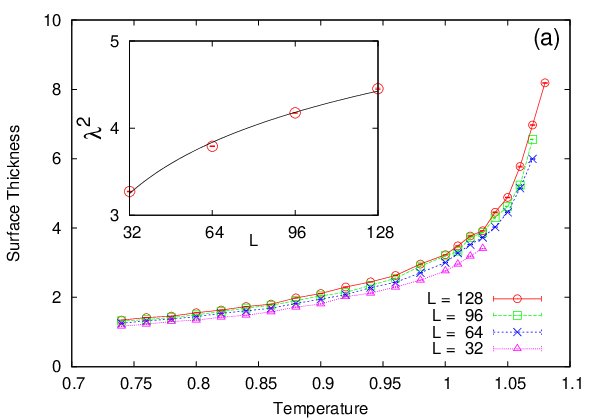
We also study the critical behavior of the interface thickness. We find that the interface thickness exhibits strong finite-size effect as shown in Fig. 8 (a), while the finite-size effect on the the surface tension is almost negligible. These finite-size dependencies come from the interface broadening due to the capillary waves [36, 37]. According to the capillary wave theory, the system size dependence of the interface thickness $\lambda$ is expressed to be,

\lambda^{2}=C+\frac{T}{4\gamma}\ln L,

(12)

where $C$ is a system-size independent constant for a fixed temperature. Note that, the temperature $T$ and system-size $L$ used here are dimensionless values. The system-size dependence of the interface thickness for $T=0.9$ is shown in the inset of Fig. 8 (a). From this finite-size dependence, we estimate the surface tension as a function of temperature. The critical behavior of the surface tension obtained from the interface thickness is shown in Fig. 8 (b). The critical exponent of the correlation length is determined to be $\nu=0.63(4)$ which is consistent with the value of the Ising universality class.

IV Discussions

We determine the phase boundary between gas and liquid phases by achieving gas-liquid coexisting state with MD. This method is simple and provides the phase boundary between liquid and gas phases with high accuracy. Since we have gas-liquid interface in the system, we can check the finite-size effect on the obtained results; if the linear length of the system $L_{z}$ is much longer than the interface thickness $\lambda$ , then the coexisting densities of liquid and gas are expected to be free from the finite-size effect. In our experience, the finite-size effect on the coexisting density is vanished when $L_{z}>10\lambda$ . We determine the critical temperature from the block density analysis of the Binder parameter, which allows us to perform finite-size analysis only from one simulation run with large system size. Additionally, this method does not require the distribution of order parameter of Ising model at the criticality, and therefore, we do not have to consider the mixed-field theory.

The critical exponents $\beta$ and $\nu$ are determined from the behaviors of the order parameter and the surface tension. While the critical exponents of the order parameter $\beta$ is consistent with the Ising universality class, the exponent of correlation length $\nu$ obtained from the surface tension is found to be slightly larger than that of the Ising universality. While this deviation can be due to the capillary waves, it is difficult to remove the effect since the surface tension does not exhibit apparent finite-size effect. Potoff and Panagiotopoulos studied the critical behavior of the surface tension using HR technique and FSS analyses, and reported $\nu=0.71(4)$ which is much larger than the Ising universality [38]. However, they did not consider the effect from the capillary waves. Considering the effect of the capillary waves, we obtained the critical exponent of the correlation length $\nu=0.63(4)$ which is consistent with the Ising universality. Note that, the statistical error became larger than that of the value obtained directly from the stress tensor using Eq. (4). This is because the surface tension analysis with considering the capillary waves requires two steps; first measuring the surface thicknesses for various system sizes and then extracting the surface tension from its size dependence. While the obtained values of exponents are consistent with that of the Ising universality class, it is still difficult to declare that the universality class of the LJ system belongs to the Ising universality since the accuracy is insufficient especially for the exponent of the correlation length. Some techniques are required which can estimate the surface tension accurately. Also the distances from the criticality is insufficient enough to discuss the universality class precisely. In order to get closer to the critical point, larger and longer simulations are necessary. It should be one of the further issues.

Some of the past studies reported the effect from the correction to scaling [20, 21]. They first obtained the apparent critical temperatures for several system size, and they took the infinite size limit considering the correction. However, we did not find any sign of the correction to scaling in Fig. 6. It is difficult to determine the value of the correction to scaling exponent if it exists. While the obtained values of critical exponents are consistent with the Ising universality without considering the correction, it would become more important in order to investigate more accurately.

Very recently, Ma and Hu [39, 40, 41, 42, 43] used MD to study relaxation and aggregation of polymer chains, in which neighboring monomers of a polymer chain are connected by rigid bonds [39, 41] or springs with various spring constants [40, 42]. They found that when the bending-angle depending potential and the torsion-angle depending potential are zero or very small, polymer chains tend to aggregate [41, 42, 43]. Such results are useful for understanding mechanism of protein aggregation [41, 42] related to neurodegenerative diseases, including Alzheimer’s disease (AD), Huntington’s disease (HD), Parkinson’s disease (PD), etc. One may argue that polymer chains can aggregate only when they are inside the phase boundary. It is of interest to extend the method of the present paper to calculate the phase diagram to calculate phase diagrams of polymer chains of various chain lengths [44]. Such phase diagrams will be useful for understanding under what temperature and density conditions, polymer chains would aggregate.

Acknowledgements

The computation was carried out by using facilities of the Supercomputer Center, Institute for Solid State Physics, University of Tokyo, and Information Technology Center, Nagoya University. We would like to thank K. Binder, N. Kawashima, S. Todo, and Y. Tomita for helpful discussions. This work was partially supported by Grants-in-Aid for Scientific Research (Contract No. 23740287), by KAUST GRP (KUK-I1-005-04), by Grants NSC 100-2112-M-001-003-MY2, and by NCTS (North).

References

[1] H. E. Stanley, Introduction to Phase Transitions and Critical Phenomena (Oxford Univ. Press, New York 1971).
[2] L. P. Kadanoff, Physica A, 163, 1 (1990)
[3] E. A. Guggenheim, J. Chem. Phys. 13, 253(1945).
[4] More recent experimental results for liquid-gas critical systems can be found in the paper V. Privman, P. C. Hohenberg and A. Aharony in Phase Transitions and Critical Phenomena: V. 14 edited by C. Domb and J.L. Lebowitz and C. Domb (Academic Press, London, 1991).
[5] B. M. Magnetti, et al., J. Chem. Phys. 130, 044101 (2009).
[6] L. Onsager, Phys. Rev. 65, 117(1944).
[7] F. G. Wang and C.-K. Hu, Phys. Rev. E 56, 2310 (1997).
[8] D. Stauffer and A. Aharony, Introduction to Percolation Theory, Revised 2nd. ed. (Taylor and Francis, London, 1994).
[9] C.-K. Hu, C.-Y. Lin, and J.-A. Chen, Phys. Rev. Lett. 75, 193 (1995) and 75, 2786(E) (1995); Physica A 221, 80 (1995)
[10] C.-K. Hu and C.-Y. Lin, Phys. Rev. Lett. 77, 8 (1996).
[11] H. Watanabe, S. Yukawa, N. Ito, and C.-K. Hu, Phys. Rev. Lett. 93, 19601 (2004). This paper contains some typos, see Ref. [12] for details; see also G. Pruessner and N. R. Moloney, Phys. Rev. Lett. 95, 258901 (2005).
[12] H. Watanabe and C.-K. Hu, Phys. Rev. Lett. 95, 258902 (2005); Phys. Rev. E 78, 041131 (2008).
[13] N. Sh. Izmailian, V. B. Priezzhev, P. Ruelle, and C.-K. Hu, Phys. Rev. Lett. 95, 260602 (2005); N. Sh. Izmailian, K. B. Oganesyan, M.-C. Wu, and C.-K. Hu, Phys. Rev. E 73, 016128 (2006).
[14] C. N. Yang and T. D. Lee, Phys. Rev. 87, 404 (1952); T. D. Lee and C. N. Yang, 87, 410 (1952).
[15] H. Watanabe, M. Suzuki, and N. Ito, Phys. Rev. E 82, 051604 (2010).
[16] A. Z. Panagiotopoulos, Mol. Phys. 61, 813 (1987); A. Z. Panagiotopoulos, J. Phys.: Condens. Matter 12, R25 (2000) .
[17] D. Möller and J. Fischer, Mol. Phys. 69, 463 (1990).
[18] B. Widom, J. Chem. Phys., 39, 2808 (1963).
[19] H. Okumura and F. Yonezawa, J. Chem. Phys. 113, 9162 (2000); H. Okumura and F. Yonezawa, J. Phys. Soc. Jpn. 70, 1990 (2001).
[20] N. B. Wilding and A. D. Bruce, J. Phys.: Condens. matter 4 3087 (1992); N. B. Wilding, Phys. Rev. E 52, 602 (1995).
[21] J. Pérez-Pellitero, P. Ungerer, G. Orkoulas, and A. D. Mackie, J. Chem. Phys. 125, 054515 (2006).
[22] A. L. Talapov and H. W. J. Bl $\ddot{o}$ te, J. Phys. A: Math. Gen. 29, 5727 (1996).
[23] N. Ito, K. Hukushima, K. Ogawa, and Y. Ozeki, J. Phys. Soc. Jpn. 69, 1931 (2000).
[24] M. Hasenbusch, Phys. Rev. B 82 174433 (2010).
[25] S. D. Stoddard and J. Ford, Phys. Rev. A 8, 1504 (1973).
[26] W. G. Hoover, Phys. Rev. A 31, 1695 (1985).
[27] M. Tuckerman, B. J. Berne, and G. J. Martyna, J. Chem. Phys. 97, 1990 (1992).
[28] http://mdacp.sourceforge.net/
[29] H. Watanabe, M. Suzuki, and N. Ito, Prog. Theor. Phys. 126, 203-235 (2011).
[30] J. A. McLennan, Introduction to Non-equilibrium Statistical Mechanics (Prentice Hall, 1996) .
[31] K. Binder, Z. Phys. B: Condens. Matter 43, 119 (1981).
[32] M. Rovere, D. W. Hermann, and K. Binder, Europhys. Lett., 6 585 (1988).
[33] J. A. Zollweg and G. W. Mulholland, J. Chem. Phys. 57, 1021 (1972); A. B. Cornfeld and H. Y. Carr, Phys. Rev. Lett. 29, 28 (1972); A. Z. Panagiotopoulos, Int. J. Thermophys. 15, 1057 (1994).
[34] J. Wang and M. A. Anisimov, Phys. Rev. E 75, 051107 (2007).
[35] M. W. Pestak, R. E. Goldstein, M. H. W. Chan, J. R. de Bruyn, D. A. Balzarini, and N. W. Ashcroft, Phys. Rev. B 36 599 (1987).
[36] W. Werner, F. Schmid, M. Müller, and K. Binder, Phys. Rev. E, 59, 728 (1999).
[37] R. L. C. Vink, J. Horbach, and K. Binder, J. Chem. Phys., 122, 134905 (2005).
[38] J. J. Potoff and A. Z. Panagiotopoulos, J. Chem. Phys., 112, 6411 (2000).
[39] W.-J. Ma and C.-K. Hu, J. Phys. Soc. Jpn 79, 024005 (2010).
[40] W.-J. Ma and C.-K. Hu, J. Phys. Soc. Jpn 79, 024006 (2010).
[41] W.-J. Ma and C.-K. Hu, J. Phys. Soc. Jpn 79, 054001 (2010).
[42] W.-J. Ma and C.-K. Hu, J. Phys. Soc. Jpn 79, 104002 (2010).
[43] C.-K. Hu and W.-J. Ma, Prog. Theor. Phys. Supp. 184, 369 (2010).
[44] Please note that Ref. [5] contains some phase diagrams of chain molecules.