Numerical studies of the ABJM theory for arbitrary at arbitrary coupling constant
Abstract:
We show that the ABJM theory, which is an superconformal Chern-Simons gauge theory, can be studied for arbitrary at arbitrary coupling constant by applying a simple Monte Carlo method to the matrix model that can be derived from the theory by using the localization technique. This opens up the possibility of probing the quantum aspects of M-theory and testing the duality at the quantum level. Here we calculate the free energy, and confirm the scaling in the M-theory limit predicted from the gravity side. We also find that our results nicely interpolate the analytical formulae proposed previously in the M-theory and type IIA regimes. Furthermore, we show that some results obtained by the Fermi gas approach can be clearly understood from the constant map contribution obtained by the genus expansion. The method can be easily generalized to the calculations of BPS operators and to other theories that reduce to matrix models.
Keywords:
AdS-CFT correspondence, Gauge-gravity correspondence, M-theory1 Introduction
Three-dimensional gauge theories with a Chern-Simons term have been studied extensively for their rich and beautiful mathematical structure [1] and for applications to quantum Hall systems in condensed matter physics. Their relevance to superstring/M-theory was realized in 2004 [2] by the appreciation that superconformal Chern-Simons theories coupled to matter fields capture the dynamics of M-theory on a multiple M2-brane background. The latter theory is expected to be obtained as an infrared fixed point of type IIA superstring theory on a D2-brane background, whose low-energy description is given by the maximally supersymmetric -dimensional Yang-Mills theory. In 2008, an explicit form of the Chern-Simons theory that describes the infrared fixed point was proposed by Aharony, Bergman, Jafferis and Maldacena (ABJM) [3], following important earlier works [4, 5]. It is a theory with Chern-Simons levels and coupled to bifundamental matters. The on-shell supersymmetric Lagrangian of the theory is given by
| (4) |
where and are gauge fields, and and are bosonic and fermionic complex bifundamental fields, respectively. This theory has supersymmetry for and supersymmetry for . It has been conjectured to be dual to M-theory on for , and to type IIA superstring on in the planar large- limit with the ’t Hooft coupling constant kept fixed.
From the viewpoint of quantum gravity, the ABJM theory is important since it may provide us with a nonperturbative definition of type IIA superstring theory or M-theory on backgrounds since the theory is well-defined for finite . One may draw a precise analogy with the way maximally supersymmetric Yang-Mills theories may provide us with nonperturbative formulations of type IIA/IIB superstring theories on D-brane backgrounds through the gauge/gravity duality [6, 7, 8, 9]. In particular, the M-theory limit is important given that M-theory is not defined even perturbatively, although there is a well-known conjecture on its nonperturbative formulation in the infinite momentum frame in terms of matrix quantum mechanics [10]. The planar limit, which corresponds to type IIA superstring theory, has interest on its own since it may allow us to perform more detailed tests of the gauge/gravity duality than in the case of . In particular, we may hope to calculate the corrections to the planar limit, which enables us to test the gauge/gravity duality at the quantum string level, little of which is known so far.
In all these prospectives, one needs to study the ABJM theory in the strong coupling regime. As in the case of QCD, it would be nice if one could study the ABJM theory on a lattice by Monte Carlo methods. This seems quite difficult, though, for the following three reasons. Firstly, the construction of the Chern-Simons term on the lattice is not straightforward, although there is a proposal [11, 12] based on its connection to the parity anomaly. Secondly, the Chern-Simons term is purely imaginary in the Euclidean formulation, which causes a technical problem known as the sign problem when one tries to apply the idea of importance sampling. Thirdly, the lattice discretization necessarily breaks supersymmetry, and one needs to restore it in the continuum limit by fine-tuning the coupling constants of the supersymmetry breaking relevant operators. (See, for instance, ref. [13].) This might, however, be overcome by the use of a non-lattice regularization of the ABJM theory [14] based on the large- reduction on [15, 16], which is shown to be useful in studying the planar limit of the 4d super Yang-Mills theory [17, 18, 19].
What we do here instead is to apply Monte Carlo methods not to the original theory (4) but to a matrix model obtained after a huge reduction of the degrees of freedom due to supersymmetry. In fact, it has been known for a while in certain supersymmetric theories that one can reduce the path integral to a finite dimensional matrix model by using the so-called localization technique. Such a technique was applied [20] to 4d super Yang-Mills theory, and some conjecture on the half-BPS Wilson loops11 1 This formula is also reproduced by a numerical simulation in the large- limit [17, 18]. [21, 22] has been confirmed. In ref. [23], the same technique has been applied to the ABJM theory on three-sphere , and its partition function was shown to reduce to a matrix integral
| (5) | |||||
which is commonly referred to as the ABJM matrix model.22 2 The localization of the ABJM theory and related theories on various manifolds such as [24], [25] and squashed [26] has also been considered. By using this matrix model, the free energy of the ABJM theory has been studied intensively [28, 29, 30, 31, 32, 33, 34, 35]. In ref. [29] the planar limit and the corrections33 3 There is also a study of non-planar corrections to anomalous dimensions by the integrability approach. See e.g., [27]. around it have been studied employing a technique from topological string theory, and the on-shell action of the type IIA supergravity on has been reproduced. In ref. [30] the free energy in the M-theory limit has been obtained using some ansatz for the eigenvalue distribution. In ref. [33] the genus expansion at strong ’t Hooft coupling has been considered and a resummed form was obtained in terms of the Airy function by using the holomorphic anomaly equation [36]. The obtained simple form was claimed to be valid to all orders in the genus expansion up to the worldsheet instanton effect. In ref. [35], the free energy in the M-theory regime at small has been calculated by the Fermi gas approach, and the result turns out to be given by the Airy function obtained in ref. [33] with some extra terms. These results, if correct, would enable us to shed light on the dynamical aspects of M-theory and to test the AdS/CFT duality including the string loop effect by studying the gravity side further.
In this paper we show that the ABJM matrix model can be rewritten in a form suitable for Monte Carlo simulations, which enables simple calculation of the partition function and BPS operators for arbitrary values of the rank and the level from first principles. In particular, we calculate the partition function explicitly for various and , which is supposed to contain the nonperturbative effects corresponding to the worldsheet instantons in string theory neglected in refs. [29, 33]. We find the well-known constant map contribution [36, 37, 38] is also correctly reproduced. The constant map contributions are of the order of , where is the genus. Note that these terms depend on the string coupling44 4 This is the string coupling in the context of topological string theory. The string coupling in the IIA superstring limit of the ABJM theory is . but not on the ’t Hooft coupling constant. In the planar limit, they correspond to a constant shift of the free energy, which becomes negligibly small in the large ’t Hooft coupling limit, and hence they do not spoil the agreement with the type IIA supergravity. They are negligible in the eleven-dimensional supergravity limit as well. However, when one considers quantum strings or M-theory, these terms should be taken into account since they have an explicit dependence. In fact, these terms become dominant at strong ’t Hooft coupling for .
This paper is organized as follows. In section 2 we review the previous results for the free energy of the ABJM matrix model in various limits, which are obtained by analytical methods. In section 3 we describe our numerical method. In section 4 we present our results, and discuss the discrepancies from the analytical results. In section 5 we show that these discrepancies can be interpreted as the constant map contributions. Section 6 is devoted to a summary and discussions. In Appendix A we explain the basics and some details of Monte Carlo simulation. In Appendix B we derive an alternative form of the ABJM matrix model, which is suitable for Monte Carlo simulation. In appendix C we show the equivalence between the constant map contribution and the Fermi gas result , which is derived by the large- and small- expansions, respectively.
Note added.
After the first version appeared on the arXiv, we were informed by Marcos Mariño that the discrepancies observed at genus 0, 1 and 2 between our numerical results and the formula proposed in ref. [33] can be naturally attributed to the constant map contributions. We greatly appreciate this important comment, which enabled us to deepen our argument in section 5.2.
2 Previous analytical results for the free energy
In this section we summarize some known analytical results for free energy of the ABJM theory, which is defined in terms of the partition function (5) as
| (6) |
2.1 Perturbative results for all
The free energy can be calculated by using a usual perturbative technique, and the result at the one-loop level is given as (See, for example, ref. [32].)
| (7) | |||||
| (8) |
where is the Barnes G-function . The -expansion is shown in the second line with Riemann’s zeta function and the Bernoulli numbers . The O() terms in (8) agree with the result (10) obtained in the planar limit. Note, however, that the expression (7) includes contributions to all orders in the -expansion.
2.2 with arbitrary
An exact expression for is obtained by Okuyama [34] as55 5 Note that the normalization of the partition function adopted in ref. [34] differs from ours as .
| (9) |
This result has been obtained by direct integration of (67). Since the expressions for the odd and even cases are different, the analyticity in (when one regards or equivalently the ’t Hooft coupling constant as a continuous variable) is not obvious a priori. However, as we will see in section 4, our numerical results suggest that the free energy is a smooth function of . The analyticity is important in the context of the AdS/CFT correspondence, in which one assumes the analyticity on the gravity side. Also the analysis in the planar limit usually assumes the analyticity implicitly.
2.3 Planar limit ( with fixed)
The free energy in the planar limit ( with fixed) has been calculated by Drukker, Marino and Putrov (DMP) [29]. These results have been obtained by a standard matrix model technique after the analytic continuation [28] to the lens space matrix model [39, 40], which is obtained from the pure Chern-Simons theory on . The validity of the analytic continuation is proved diagramatically in refs. [41, 42].
At weak coupling () the authors obtain
| (10) |
up to .
At strong coupling () the authors obtain
| (11) |
to all orders of the expansion. The leading behavior agrees with the dual type IIA supergravity prediction [29, 43] including the overall coefficient. It has been claimed that the free energy (11) at strong coupling receives the correction of the form
where is a polynomial in of degree (for ). This exponentially small correction has been interpreted in ref. [29] as the effect of the worldsheet instanton in the dual type IIA superstring, which corresponds to a string worldsheet wrapping a cycle in [45].
In section 4 we will show that another contribution of the order of O() due to the constant map needs to be added in comparing with precise numerical analysis. Although this term does not affect the agreement with supergravity, it must be taken into account when one compares the finite corrections with the string corrections.
2.4 M-theory limit ( with fixed)
In ref. [30], the free energy in the M-theory limit66 6 Strictly speaking, since the ABJM theory has been conjectured to be dual to the M-theory for , the limit with fixed is merely a sufficient condition. In the following, however, we simply call it “the M-theory limit”. ( with fixed) has been calculated and confirmed the prediction
| (12) |
from the dual eleven-dimensional supergravity, which shows the well-known scaling for the degrees of freedom in the theory of M2-branes [44]. Note also that (12) agrees with what one obtains formally from the leading large- behavior of the planar result (11) by replacing with .
The result (12) was obtained by imposing an ansatz for the eigenvalue distribution
which is necessary for the cancellation of long-range forces, and is also suggested by numerical studies of the saddle point equation. The parameter is chosen to be by requiring that all the short-range forces contribute to the free energy at the same order of in order to have nontrivial solutions.
2.5 expansion around the planar limit
Fuji, Hirano and Moriyama (FHM) [33] studied the free energy to all orders in the genus expansion neglecting the instanton contribution, which is of the order of . Their proposal for a resummed form is given by
| (13) |
where is the Airy function, and the “renormalized ’t Hooft coupling” is given by
| (14) |
The appearance of the Airy function [33] is also encountered in the context of M-theory flux compactification [46]. Note that the expression (13) reproduces (11) in the large- limit as one can easily see by using the asymptotic formula for . In section 4 we will show that (13) has another contribution, which is necessary for comparison with our numerical results.
The free energy at higher genus has been studied earlier [29, 31] by using a topological string technique after analytic continuation to the lens space matrix model. The analysis in ref. [33] has been performed by using the holomorphic anomaly equation [36], whose solution is the same as the one for the loop equation [47, 48] with some appropriate boundary conditions. In order to solve the holomorphic anomaly equation, one needs to provide some inputs such as the free energy at genus zero and one, which are taken to be
In this way the authors have found a general solution, which gives the free energy at all genus up to the worldsheet instanton effect. The integration constants were determined by assuming the absence of non-perturbative corrections of the type . Strictly speaking, what one obtains in this way is the “weight zero” contribution to the free energy in the language of topological string theory. It is claimed that one can turn this result into the one including contributions from all weights by making a replacement , which is given in (14).
This “renormalized ’t Hooft coupling” is different from the expectation from the gravity side [49] : . While it is possible that this disagreement may imply that the AdS/CFT does not hold at finite-/quantum string level, we should definitely gain more understanding on both gauge theory and gravity sides. The additional contribution to the FHM result from the constant map should be important also from this point of view.
2.6 , small
In ref. [35], the free energy with fixed small has been calculated by using the Fermi gas approach neglecting the quantum mechanical instanton effect (worldsheet instanton) and the terms which are suppressed exponentially at large (membrane instanton). In this approach, the partition function of the ABJM theory is regarded as an ideal Fermi gas system described by (65) with the Planck constant identified as . The result is given by
| (15) |
The leading large- behavior reproduces eq. (12) exactly. The function in (15) is given for as77 7 Although the Chern-Simons level must be integer in a physical setup, the integral (5) is itself well-defined also for non-integer and we can actually obtain numerical results, which turn out to be a smooth function of .
| (16) |
Since the first term in (15) can be obtained formally from the FHM result in (13) by replacing with , one can rewrite it as
| (17) |
where may be viewed as “quantum corrections” with the “Planck constant” . Note that the first term in (17) is valid for all although (16) is obtained at small . The authors note that the second and third terms in (16) are given by
| (18) | |||||
for . This is the power series with odd powers of unlike the usual genus expansion around the planar limit. The authors suggest that may encode the effect from D0-branes of the order of .
3 Numerical methods for the ABJM matrix model at arbitrary and
In this section we discuss how we can study the ABJM matrix model at arbitrary and by applying a standard Monte Carlo method. For the readers who are not familiar with Monte Carlo methods in general, we review the basic ideas in Appendix A. For an earlier work on Monte Carlo simulation of a one-matrix model, see ref. [50].
The ABJM matrix model in the form (5) is not suitable for Monte Carlo simulation since the integrand is not real positive.88 8 One might think of simulating a system without the phase factor , and including its effect afterwards by reweighting. While it is possible to obtain results for the case along this line, the calculation becomes more and more difficult for larger due to the sign problem. However, as we review in Appendix B in detail, one can rewrite the ABJM matrix model as follows.
| (19) |
In the case, one may view (19) as a mirror description of the ABJM theory in terms of the 3d SYM with adjoint and fundamental hypermultiplets, which is isomorphic to 3d SYM in the low-energy limit [51]. The important point here is that, in this form (19), the integrand is real positive, and we can perform Monte Carlo simulation in a straightforward manner as described in Appendix A.
We should also note that, while the level should be an integer in the original 3d gauge theory, nothing prevents us from considering non-integer in the integral (5). In what follows, we therefore extend the value of to any real number.
In order to calculate the free energy (6), which is the log of the partition function, we need to rewrite it in terms of expectation values of some quantities, which are directly calculable by Monte Carlo methods.99 9 For applications of such an idea on different supersymmetric systems, see refs. [52] and [53]. The basic idea in our case is to calculate the ratios of the partition functions for different or as expectation values. Since we know the results for or , we can obtain results for arbitrary and by calculating an appropriate product of the ratios. Depending on whether we change or , we have the following two methods, which give the same result within statistical errors as we have checked for various and . The second method is particularly useful in studying the M-theory limit, which corresponds to the large limit with fixed .
3.1 Calculating the ratio of partition functions with different
Let us consider a trivial identity
| (20) |
where we have defined
| (21) |
and stands for the expectation value with respect to the action
| (22) |
The quantity (20) can be calculated easily by the standard Monte Carlo method as far as and are sufficiently close.1010 10 As moves away from , the quantity fluctuate violently during the simulation of the system , which leads to larger statistical errors. Therefore, we can calculate the free energy as
| (23) | |||||
where and we have used in the last line. We have to make the adjacent values of close enough for the reason mentioned above.
3.2 Calculating the ratio of partition functions with different
Let us decompose into and consider the ratio
| (24) | |||||
where the symbol denotes the expectation value with respect to the “action” . Note that
| (25) |
due to the factorization of the potential terms. In order to calculate the right-hand side of (24) with good accuracy, it is necessary to take small enough to make sure that (25) does not fluctuate violently during the simulation. In actual calculation we use . Then by calculating (24) for , and by using the result
| (26) |
we can calculate the free energy for successively with a fixed value of .
4 Results for the free energy

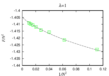
In this section we present our numerical result for the free energy of the ABJM theory. In order to test our code, we first study the case and compare our result against the exact result (9) obtained by Okuyama [34]. As can be seen from fig. 1, our result reproduces the exact result very accurately. We have also obtained results for non-integer values of , which are not obtained in ref. [34]. They are found to connect the results for integer smoothly.
4.1 Planar limit
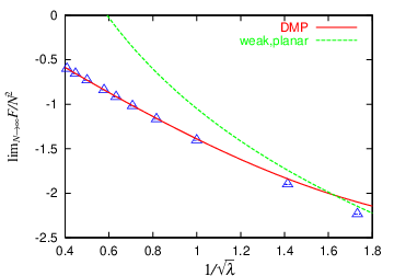
Next we consider the planar limit ( with fixed), which is conjectured to be dual to the classical type IIA superstring on . In fig. 2 we plot the normalized free energy against for various values of . Our results can be fitted well by as theoretically expected1111 11 The functions and defined here are related to and , which are defined in (29), as and . . In the left panel of fig. 3, we plot against . The results seem to interpolate the DMP result (11) at strong coupling and the perturbative result (10) at weak coupling. However, by looking more carefully into the asymptotic behavior for large , we find certain discrepancies. This can be seen from the right panel of fig. 3, in which we plot the difference , which is found to behave as
| (27) | |||
| (28) |
instead of the behavior expected from the worldsheet instanton effect. We consider that is consistent with zero since the fitting error may well be slightly underestimated. Since the discrepancy (27) vanishes at (assuming that in (27) is zero), it does not affect the agreement with the dual type IIA supergravity.
In section 5 we explain that this discrepancy can be understood as the constant map at genus . Similar discrepancies exist also in corrections around the planar limit as we will see.


4.2 M-theory limit
Next we consider the large- limit with fixed , which is conjectured to correspond to the eleven dimensional supergravity on . Figure 4 shows that the free energy grows in magnitude as with , and behaves as , which enables us to obtain the M-theory limit reliably.


In fig. 5 we plot against , which confirms the prediction (12) from eleven-dimensional supergravity for very precisely.

4.3 Finite effects
One of the important results on finite effects in the free energy is that the corrections around the planar limit are resummed in a closed form (13) neglecting the worldsheet instanton effect. In fig. 6 we plot our results for and and compare them with the FHM result (13) and the DMP result (11). We find that both FHM and DMP are close to our data at strong coupling, but the difference between them is too small to see whether FHM is doing any better than DMP. This is simply because the term (12), which commonly exists in both results, is dominating over the difference. We therefore plot against for (Left) and (Right) in fig. 7. The leading large- behavior of the plotted quantity is for FHM and for DMP, where the difference comes from the term in (14). The difference becomes negligible for , but it is significant for , in which case our data are indeed closer to FHM than to DMP.


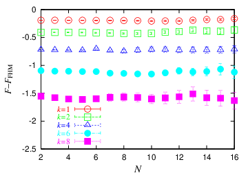
We also find some discrepancy between our result and FHM, which are almost independent of . To see it more directly, we plot in fig. 8 the difference between our result and the FHM result for various . It turns out that the discrepancies are indeed almost independent of . This strongly suggests that the FHM result correctly incorporates the finite effects except for a term which depends only on . Note that this discrepancy cannot be explained by the worldsheet instanton effect , which is neglected in FHM. While this discrepancy does not affect the M-theory limit corresponding to the strict limit for fixed , it is non-negligible when one considers corrections. As we will see in section 5, this discrepancy coincides with in eq. (17) by Fermi gas approach [35] for small and with the constant map contribution for all .
5 Interpretation of the discrepancies
In this section we provide an interpretation of the discrepancies between our data and the known analytical results, which we observe in the previous section.
5.1 Genus expansion
Let us consider the planar limit, in which is kept fixed. In that limit, the free energy can be expanded with respect to the genus as
| (29) | |||||
Below we consider the free energy order by order in this expansion.
Planar contribution
The planar contribution can be studied by the saddle point method, and the can be determined by solving [28, 29, 32, 54]
| (32) |
where is the Meijer G-function1212 12 The Meijer G-function is defined by where the path is chosen in an appropriate way depending on the parameters. See, for instance, ref. [55] for the details. and is the hypergeometric function. Note that these equations are exact for arbitrary , and hence they fully incorporate the worldsheet instanton effect. One can obtain by carrying out the integration over as
| (33) |
At weak coupling , in particular, one obtains
| (34) | |||||
| (35) |
By comparing this with the perturbative calculation (10), one finds .
At strong coupling , one obtains
| (36) | |||||
| (37) | |||||
where . Here is an “integration constant”, which has been set zero in the previous works, for instance, in ref. [29], which leads to eq. (11).
In fig. 9 we plot , where is evaluated numerically by performing the integral (33) explicitly. As increases, we find that approaches a nonzero constant
| (38) |
which coincides with obtained as the constant map contribution at genus zero [36, 37, 38]. The value of in (27) predicted from the above calculation is , which agrees well with the discrepancy (28) observed in the planar limit.

Higher genus contributions
Next we discuss the discrepancy at higher genus, which can be also interpreted as the constant map contributions as in the planar part. Let us note that the analytical results up to the constant map have been obtained for genus one and two in terms of modular forms as [29, 31, 48, 56]
| (39) | |||||
| (40) | |||||
where is the Dedekind eta function, is the Eisenstein series of weight , is the theta function, and is defined as
| (41) |
where is the complete elliptic integral of the first kind.


In fig. 10 we plot (Left) and (Right) against , where we have defined the weak coupling results
| (42) | |||||
| (43) |
at genus one and two, respectively, as can be read off from (8). We find in both cases that the result approaches a constant as , which gives
| (44) |
respectively. This suggests that in the weak coupling region there are additional terms given by
| (45) |
which precisely coincide with the constant map contributions [36, 37, 38]
| (46) |
Since the FHM result (13) reproduces the previous results in the genus expansion, the FHM result must also have the additional contributions
| (47) |
where the worldsheet instanton effect is neglected.
As we did in the case of planar contribution, we can test whether the discrepancy in the genus one contribution between our data and the previous analytical results can be explained by the additional terms identified above. In fig. 11 we extract the genus one contribution from our data in the following way. First we subtract from our data for the free energy, the planar contribution , where is obtained by (33), and subtract also the term that appears in the weak coupling result (42). Then we plot the result after these subtractions against in fig. 11 (Left), which can be nicely fitted to straight lines. The intercepts give the values of the genus one contribution for each , which are plotted against in fig. 11 (Right). We find that the result is in good agreement with the genus one contribution of after making a constant shift by determined as (44).


5.2 Finite effects
Let us see how well the FHM result with the corrections (47) does at finite . In fig. 12 we plot , i.e., the discrepancies between our result and the FHM result for and against . At , the data and the data are on top of each other as anticipated from fig. 8. In this regime, the discrepancies are in good agreement with the corrections (47) identified in section 5.1.
It is interesting to see what happens if we go to smaller region in fig. 12 although non-integer is not physical in the original gauge theory. Firstly we start to see some difference between and , which implies that there is some dependence which is not captured by the FHM result in this regime. We speculate that the dependence is due to the membrane instanton effect [31, 57], which behaves as , since the worldsheet instanton effect is negligible in this regime. Secondly, we find that the discrepancy between our result and the FHM result no longer agrees with (47) including corrections up to genus two. This is understandable since the higher genus terms become non-negligible as one goes to smaller (larger ).
On the other hand, the free energy at small is calculated by the Fermi gas approach as (17). We find that our data for interpolate nicely the behavior (17) at small and the behavior (47) at large . This also supports our speculation that the difference between the and data at small is due to the membrane instanton effect, which is neglected in the Fermi gas approach. Note, in particular, that the Fermi gas approach yields correction to the FHM result in odd powers of , whereas the genus expansion yields even powers of . Our data nicely interpolate the two asymptotic behaviors, which are smoothly connected around .


Finally let us consider the sum of the constant map contributions at all genus (46), which is given by1313 13 An assumption is needed to obtain (48) and (49). For details, see appendix C.
| (48) | |||||
In fig. 12 we find that this function agrees well with the discrepancy between our result and the FHM result for the whole range of investigated, including . Since the Fermi gas result (17) also gives accurate description there, it is natural to guess that they are actually the same. Indeed, as we show in appendix C, the sum of the constant map (48) can be expanded around as
| (49) | |||||
which exactly reproduces the result of the Fermi gas approach (17) to the term.1414 14 Note that the Fermi gas calculation has been done only to the term, and the higher order terms are just an educated guess. Calculations at higher orders would be an interesting future direction. Remarkably, the constant map contribution (48) and the expansion (49) are equivalent at any . Therefore, we expect that the result (49) is the all-order form of in the Fermi gas approach. In other words, we expect that the expansions of the free energy around (the constant map contribution) and (the Fermi gas approach) give the same answer after taking sums to all orders. In this sense the free energy around the planar and M-theory limits are smoothly connected with each other.
6 Summary and discussions
In this paper we have established a simple numerical method for studying the ABJM theory on a three sphere for arbitrary rank at arbitrary Chern-Simons level . The crucial point is that we are able to rewrite the ABJM matrix model, which is obtained after applying the localization technique, in such a way that the integrand becomes positive definite. By using this method, we have confirmed from first principles that the free energy in the M-theory limit grows proportionally to as predicted from the eleven-dimensional supergravity. We have also found that the FHM formula with the additional terms describes the free energy of the ABJM theory in the type IIA superstring and M-theory regimes. Analytic form of the additional terms is discussed in detail, and beautiful agreement between planar and M-theory regions is found. These additional terms become important when we consider the quantum string effect in the AdS/CFT duality.
There are many issues worth being addressed by using our method. Most importantly from the conceptual point of view, we can use the free energy obtained for finite and finite to test the AdS/CFT duality at the quantum string level. At the tree level, or equivalently in the planar limit, there is strong evidence that the gauge theory correctly describes the string effect. For example, the D0-brane quantum mechanics reproduces the correction to the black 0-brane solution in type IIA superstring theory [60]. However, no definite conclusion is obtained for quantum string corrections so far. In fact, as pointed out in ref. [33], the FHM formula does not seem to agree with a prediction from the string theory side [49]. This disagreement is not solved even if we take into account of the corrections found in this paper. Some of the possible solutions to this puzzle includes: (i) one has to consider some different gauge theory such as theory, which gives different corrections, (ii) one has to refine the argument on the string theory side, and (iii) the AdS/CFT does not hold at the quantum string level. In particular, the scenario (i) can be tested straightforwardly by extending our method.
We consider it equally important to study quantum M-theory. While there is very little knowledge on it so far, we may hope to get some insight through intensive numerical studies of the ABJM theory. In fact similar attempts have been made recently [61, 62] using the BFSS matrix theory [10]. Numerical studies suggest that the prediction from the dual string theory for the scaling dimension of a certain class of operators continues to hold in the M-theory region. Similar or possibly more striking features of M-theory may show up by studying the ABJM theory numerically.
While we have focused on the free energy as the most fundamental quantity in the ABJM theory, our method can be used to calculate the expectation values of BPS operators. For instance, it is possible to calculate the expectation value of the circular Wilson loop for various representations. They are conjectured to be related to the string worldsheet area and the D-brane world-volume in the type IIA superstring region, respectively. It would be interesting to test this conjecture and to see the stringy corrections.
Our method can be also applied to other theories, which have recently attracted much attention in connection to the F-theorem and the entanglement entropy. For example, one can study the necklace-type quiver discussed in ref. [63]. We can also study other gauge groups such as and studied in ref. [64, 65]. Detailed studies of these theories outside the planar limit, in particular, would be very interesting. For instance, the so-called orbifold equivalence, which is usually proven to hold only in the planar limit, can hold outside the planar limit in these models [66, 67]. Note also that the ABJM matrix model is related to the lens space matrix model, which appears in the context of the topological string theory. It is therefore conceivable that there might be some applications to the topological string theory as well.
We hope that the results of this work are convincing enough to show the power of the numerical approach, and that many more applications other than those listed above would reveal themselves as we proceed further.
Acknowledgment
The authors would like to thank N. Drukker, S. Hirano, D. Honda, I. Kanamori, M. Mariño, Y. Matsuo, T. Takimi and D. Yokoyama for valuable discussions. In particular, we greatly appreciate M. Mariño’s important comment on the constant map, which was crucial in arriving at complete understanding on the correction to the FHM formula. M. Hanada, M. Honda and J. Nishimura are grateful to the hospitality of the Kavli Institute for Theoretical Physics in UCSB, during the KITP program “Novel Numerical Methods for Strongly Coupled Quantum Field Theory and Quantum Gravity”. This research was supported in part by the National Science Foundation under Grant No. PHY11-25915. M. Honda, Y. Honma and S. Shiba are supported by Grant-in-Aid for JSPS fellows (No. 22-2764, 22-3677 and 23-7749). The work of J. Nishimura is supported in part by Grant-in-Aid for Scientific Research (No. 20540286 and 23244057) from JSPS. S. Shiba would like to thank the hospitality of theoretical physics group at Imperial College London. Computations have been carried out on PC clusters at KEK Theory Center and B-factory Computer System.
Appendix A Basics and details of the Monte Carlo simulation
In this section we explain the basics and details of the Monte Carlo simulation1515 15 There are many good references on Monte Carlo methods. See, e.g., ref. [58].. Let us consider the action
| (50) |
(Below we abbreviate as .) Let be an “observable”, which is a function of . In general, it is difficult to calculate the expectation value of defined by
| (51) |
A brute force integration is not practical unless the number of variables is very small such as . Monte Carlo simulation is a practical tool, which enables this calculation even for large .
In Monte Carlo simulation, a series of configurations
| (52) |
is generated in such a way that the probability with which a configuration appears approaches as the number of configurations increases. More precisely, we require that the probability with which a configuration appears at -th step converge to as
| (53) |
Then the expectation value can be obtained by simply taking an average over the configurations as
| (54) |
This can be achieved by generating the series with a transition probability , which (neglecting a few technical details) satisfies following conditions.
- •
Markov chain. — The transition probability from to does not depend on previous configurations .
- •
Ergodicity. — For any pair of configurations and , there is nonzero transition probability within finite steps.
- •
Aperiodicity. — The probability from to is always nonzero.
- •
Positive state. --- All configurations have finite mean recurrence time1616 16 If is the probability to get from to in -steps of the Markov chain, without reaching this configuration at any intermediate step, then the mean recurrence time of is defined by . .
- •
Detailed balance. — The following equality should hold for arbitrary pairs of configurations and .
(55)
There are many ways to satisfy these conditions. In this work we use the Hybrid Monte Carlo (HMC) method [59]. We introduce fictitious momentum variables , which are conjugate to , and consider a Hamiltonian
| (56) |
Starting with an initial configuration , we generate a series of configurations by repeating the following steps:
- •
Generate randomly, with a probability weight .
- •
Starting with a configuration , get a new configuration by the “molecular dynamics” explained below.
- •
“Accept” the new configuration (i.e. take ) with a probability , where and are the value of the Hamiltonian calculated with and , respectively. When the new configuration is rejected, we keep an old configuration, so that .
The “molecular dynamics” is defined as follows. First we introduce a fictitious time and consider the time evolution according to the Hamilton equations
| (57) |
If we solve the Hamilton equations exactly, the Hamiltonian is conserved. In practice, we solve them approximately by discretizing the differential equations, so the Hamiltonian is not conserved exactly. We denote the time step as and the number of steps as . Then and are calculated by using the following “leap-frog method”, starting with and .
- •
- •
- •
- •
- •
- •
- •
- •
Note that the leap-frog method is designed so that the reversibility is satisfied. Namely, by starting with the final configuration and and reversing the time, the initial configuration and is reproduced. As a result, the detailed balance condition is satisfied.1717 17 For simplicity, let us assume . (The argument for the case with is the same.) Because of the reversibility, the transition probabilities are (58) (59) and (60) (61) Therefore, (62) (63)
In the simulation, and should be chosen so that a good approximation is achieved with fewer configurations. For that purpose, (i) the change at each transition should be sufficiently large, and (ii) the acceptance rate should be large. The first condition is achieved by taking sufficiently large. However, if we fix and take larger , the Hamiltonian is not conserved at all, and the new configurations are hardly accepted. Therefore one has to take smaller so that the conservation of the Hamiltonian becomes better. In actual simulations (at and , for example), we took and , so that the acceptance rate is around 0.8. As an initial configuration, we choose to be a random number in .
In Monte Carlo simulation, configurations with larger path-integral weight (“important samples”) appear more often. For this reason it is called also the importance sampling. Since the region of configuration space, which gives dominant contribution to the path integral is typically quite limited, a good approximation can be achieved with a rather small number of important samples. This should be contrasted to the usual brute force integration, in which most of the CPU time is wasted for calculating the integrand for unimportant configurations.
In Monte Carlo simulation, as we have described above, configurations are generated with the probability . Therefore, the Monte Carlo method works only if the path-integral weight is real and positive. If the measure is not real and positive, the model is said to suffer from the sign problem or the phase problem; here “sign” and “phase” mean the negative sign and the complex phase of the integration weight. In the original form of the ABJM matrix model (5), the partition function is given by an integration of a complex function. Therefore it suffers from the sign problem, and the Monte Carlo method is not applicable.
Appendix B Derivation of the sign-problem-free form of the ABJM matrix model
In this section we derive the sign-problem-free form of the ABJM matrix model, which was used in ref. [51, 34, 35] for a different purpose. Let us start with the ABJM matrix model (5). We are going to use the Cauchy identity1818 18 See the appendix of ref. [51] for the proof of this identity.
| (64) |
Here runs through all permutations. By setting , it becomes
From this, we obtain
Therefore, the partition function can be written as
By using the formula
we obtain
Therefore, the partition function becomes1919 19 In the Fermi gas approach [35], the integrand is identified with a partition function for the ideal Fermi gas given by (65) where is interpreted as the one-particle density matrix (66)
| (67) | |||||
We use the Cauchy identity again:
Thus we arrive at the final expression
| (68) |
which does not have a sign problem.
Appendix C The relation between the constant map and the Fermi gas result
In this appendix we show the correspondence between the constant map contribution and the Fermi gas result , which is derived by the large- and small- expansions, respectively.
As we mentioned earlier, the constant map contribution is given by
| (69) |
where the coefficients are
| (70) |
In order to evaluate the summation more easily, we use the integral representation of the Bernoulli number,
| (71) |
By using this representation, we obtain
| (72) | |||||
This summation is easily performed by using a formula
| (73) |
Note that the series converges only for . However, since the result of the summation in the right hand side is well-defined even for , we analytically continue to the whole region including and assume that this does not affect the result of the integration2020 20 Even if this assumption is not valid, the discrepancy at small is expected to be at most. .
By substituting in the formula, the summation is rewritten as
| (74) |
By changing the variable as , we obtain a simpler form,
| (75) |
Although each term of the integrand is divergent at , this is canceled with each other, and therefore the integral gives a finite value. In order to make our analysis easier, we will apply the zeta-function regularization to the integral.
For later convenience, we decompose the integral as
| (76) |
Note that the first factor in the second term is the generating function of the Bernoulli number
| (77) |
Although this series also converges only for , we analytically continue it to the whole region and assume that this does not affect the result. Then by using the formula
| (78) |
the integral rewritten as
The first integral is easily performed by using
where is the Euler-Mascheroni constant. We obtain
| (80) | |||||
Next we evaluate the second integral
- •
For
By using the formula(81) we obtain
(82) - •
For
(83) - •
For
By using the formula(84) the integral becomes
(85)
Thus the constant map contribution is rewritten as
| (86) | |||||
Since , , and , we obtain
| (87) | |||||
| (88) |
which is same as derived by the Fermi gas approach [35] up to the order of . Therefore, we expect that this is the all-order form in the Fermi gas picture if we calculate higher order of .
Thus we conclude that the constant map contribution and the term in the Fermi gas result are the series expansions of the integral representation (75) around and , respectively, with the radius of convergence being finite. In other words, the two expansions are smoothly connected with each other by analytic continuation.
References
- [1] E. Witten, “Quantum Field Theory and the Jones Polynomial,” Commun. Math. Phys. 121 (1989) 351.
- [2] J. H. Schwarz, “Superconformal Chern-Simons theories,” JHEP 0411 (2004) 078 [hep-th/0411077].
- [3] O. Aharony, O. Bergman, D. L. Jafferis and J. Maldacena, “ superconformal Chern-Simons-matter theories, M2-branes and their gravity duals,” JHEP 0810 (2008) 091 [arXiv:0806.1218 [hep-th]].
- [4] J. Bagger and N. Lambert, “Gauge symmetry and supersymmetry of multiple M2-branes,” Phys. Rev. D77 (2008) 065008 [arXiv:0711.0955 [hep-th]].
- [5] A. Gustavsson, “Algebraic structures on parallel M2-branes,” Nucl. Phys. B 811 (2009) 66 [arXiv:0709.1260 [hep-th]].
- [6] J. M. Maldacena, “The Large limit of superconformal field theories and supergravity,” Adv. Theor. Math. Phys. 2 (1998) 231 [Int. J. Theor. Phys. 38 (1999) 1113] [hep-th/9711200].
- [7] S. S. Gubser, I. R. Klebanov and A. M. Polyakov, “Gauge theory correlators from noncritical string theory,” Phys. Lett. B 428, 105 (1998) [arXiv:hep-th/9802109].
- [8] E. Witten, “Anti-de Sitter space and holography,” Adv. Theor. Math. Phys. 2, 253 (1998) [arXiv:hep-th/9802150].
- [9] N. Itzhaki, J. M. Maldacena, J. Sonnenschein and S. Yankielowicz, “Supergravity and the large limit of theories with sixteen supercharges,” Phys. Rev. D 58 (1998) 046004 [hep-th/9802042].
- [10] T. Banks, W. Fischler, S. H. Shenker and L. Susskind, “M theory as a matrix model: A Conjecture,” Phys. Rev. D 55 (1997) 5112 [hep-th/9610043].
- [11] W. Bietenholz and J. Nishimura, “Ginsparg-Wilson fermions in odd dimensions,” JHEP 0107, 015 (2001) [hep-lat/0012020].
- [12] W. Bietenholz and P. Sodano, “A Ginsparg-Wilson approach to lattice Chern-Simons theory,” hep-lat/0305006.
- [13] J. Giedt, “Progress in four-dimensional lattice supersymmetry,” Int. J. Mod. Phys. A 24, 4045 (2009) [arXiv:0903.2443 [hep-lat]].
- [14] M. Hanada, L. Mannelli and Y. Matsuo, “Large-N reduced models of supersymmetric quiver, Chern-Simons gauge theories and ABJM,” JHEP 0911, 087 (2009) [arXiv:0907.4937 [hep-th]].
- [15] T. Ishii, G. Ishiki, S. Shimasaki and A. Tsuchiya, “N=4 Super Yang-Mills from the Plane Wave Matrix Model,” Phys. Rev. D 78, 106001 (2008) [arXiv:0807.2352 [hep-th]].
- [16] H. Kawai, S. Shimasaki and A. Tsuchiya, “Large N reduction on group manifolds,” Int. J. Mod. Phys. A 25, 3389 (2010) [arXiv:0912.1456 [hep-th]].
- [17] M. Honda, G. Ishiki, J. Nishimura and A. Tsuchiya, “Testing the AdS/CFT correspondence by Monte Carlo calculation of BPS and non-BPS Wilson loops in 4d N=4 super-Yang-Mills theory,” PoS LAT 2011, 244 (2011) [arXiv:1112.4274 [hep-lat]].
- [18] J. Nishimura, “Non-lattice simulation of supersymmetric gauge theories as a probe to quantum black holes and strings,” PoS LAT 2009, 016 (2009) [arXiv:0912.0327 [hep-lat]].
- [19] M. Honda, G. Ishiki, S. -W. Kim, J. Nishimura and A. Tsuchiya, “Supersymmetry non-renormalization theorem from a computer and the AdS/CFT correspondence,” PoS LATTICE 2010, 253 (2010) [arXiv:1011.3904 [hep-lat]].
- [20] V. Pestun, “Localization of gauge theory on a four-sphere and supersymmetric Wilson loops,” arXiv:0712.2824 [hep-th].
- [21] J. K. Erickson, G. W. Semenoff and K. Zarembo, “Wilson loops in supersymmetric Yang-Mills theory,” Nucl. Phys. B 582 (2000) 155 [hep-th/0003055].
- [22] N. Drukker and D. J. Gross, “An Exact prediction of SUSYM theory for string theory,” J. Math. Phys. 42 (2001) 2896 [hep-th/0010274].
- [23] A. Kapustin, B. Willett and I. Yaakov, “Exact Results for Wilson Loops in Superconformal Chern-Simons Theories with Matter,” JHEP 1003 (2010) 089 [arXiv:0909.4559 [hep-th]].
- [24]
D. L. Jafferis,
“The Exact Superconformal R-Symmetry Extremizes Z,”
arXiv:1012.3210 [hep-th],
N. Hama, K. Hosomichi and S. Lee, “Notes on SUSY Gauge Theories on Three-Sphere,” JHEP 1103, 127 (2011) [arXiv:1012.3512 [hep-th]],
D. L. Jafferis, I. R. Klebanov, S. S. Pufu and B. R. Safdi, “Towards the F-Theorem: N=2 Field Theories on the Three-Sphere,” JHEP 1106, 102 (2011) [arXiv:1103.1181 [hep-th]]. - [25]
S. Kim,
“The Complete superconformal index for N=6 Chern-Simons theory,” Nucl. Phys. B 821, 241 (2009) [arXiv:0903.4172 [hep-th]],
Y. Imamura, D. Yokoyama and S. Yokoyama, “Superconformal index for large N quiver Chern-Simons theories,” JHEP 1108, 011 (2011) [arXiv:1102.0621 [hep-th]]. - [26]
Y. Imamura and D. Yokoyama,
“N=2 supersymmetric theories on squashed three-sphere,”
Phys. Rev. D 85, 025015 (2012) [arXiv:1109.4734 [hep-th]],
N. Hama, K. Hosomichi and S. Lee, “SUSY Gauge Theories on Squashed Three-Spheres,” JHEP 1105, 014 (2011) [arXiv:1102.4716 [hep-th]]. - [27] C. Kristjansen, M. Orselli and K. Zoubos, “Non-planar ABJM Theory and Integrability,” JHEP 0903 (2009) 037 [arXiv:0811.2150 [hep-th]].
- [28] M. Marino and P. Putrov, “Exact Results in ABJM Theory from Topological Strings,” JHEP 1006 (2010) 011 [arXiv:0912.3074 [hep-th]].
- [29] N. Drukker, M. Mariño and P. Putrov, “From weak to strong coupling in ABJM theory,” Commun. Math. Phys. 306 (2011) 511 [arXiv:1007.3837 [hep-th]].
- [30] C. P. Herzog, I. R. Klebanov, S. S. Pufu and T. Tesileanu, “Multi-Matrix Models and Tri-Sasaki Einstein Spaces,” Phys. Rev. D 83, 046001 (2011) [arXiv:1011.5487 [hep-th]].
- [31] N. Drukker, M. Mariño and P. Putrov, “Nonperturbative aspects of ABJM theory,” arXiv:1103.4844 [hep-th].
- [32] M. Mariño, “Lectures on localization and matrix models in supersymmetric Chern-Simons-matter theories,” J. Phys. A44 (2011) 463001 [arXiv:1104.0783 [hep-th]].
- [33] H. Fuji, S. Hirano and S. Moriyama, “Summing Up All Genus Free Energy of ABJM Matrix Model,” JHEP 1108 (2011) 001 [arXiv:1106.4631 [hep-th]].
- [34] K. Okuyama, “A Note on the Partition Function of ABJM theory on ,” arXiv:1110.3555 [hep-th].
- [35] M. Mariño and P. Putrov, “ABJM theory as a Fermi gas,” arXiv:1110.4066 [hep-th].
- [36] M. Bershadsky, S. Cecotti, H. Ooguri and C. Vafa, “Kodaira-Spencer theory of gravity and exact results for quantum string amplitudes,” Commun. Math. Phys. 165, 311 (1994) [hep-th/9309140].
- [37] C. Faber and R. Pandharipande, “Hodge Integrals and Gromov-Witten theory,h [math.ag/9810173].
- [38] M. Marino, S. Pasquetti and P. Putrov, “Large N duality beyond the genus expansion,” JHEP 1007, 074 (2010) [arXiv:0911.4692 [hep-th]].
- [39] M. Marino, “Chern-Simons theory, matrix integrals, and perturbative three manifold invariants,” Commun. Math. Phys. 253, 25 (2004) [hep-th/0207096].
- [40] M. Aganagic, A. Klemm, M. Marino and C. Vafa, “Matrix model as a mirror of Chern-Simons theory,” JHEP 0402, 010 (2004) [hep-th/0211098].
- [41] R. Dijkgraaf and C. Vafa, “N=1 supersymmetry, deconstruction, and bosonic gauge theories,” hep-th/0302011.
- [42] R. Dijkgraaf, S. Gukov, V. A. Kazakov and C. Vafa, “Perturbative analysis of gauged matrix models,” Phys. Rev. D 68, 045007 (2003) [hep-th/0210238].
- [43] R. Emparan, C. V. Johnson and R. C. Myers, “Surface terms as counterterms in the AdS / CFT correspondence,” Phys. Rev. D 60, 104001 (1999) [hep-th/9903238].
- [44] I. R. Klebanov and A. A. Tseytlin, “Entropy of near extremal black p-branes,” Nucl. Phys. B 475, 164 (1996) [hep-th/9604089].
- [45] A. Cagnazzo, D. Sorokin and L. Wulff, “String instanton in AdS(4) x CP**3,” JHEP 1005, 009 (2010) [arXiv:0911.5228 [hep-th]].
- [46] H. Ooguri, C. Vafa and E. P. Verlinde, “Hartle-Hawking wave-function for flux compactifications,” Lett. Math. Phys. 74, 311 (2005) [hep-th/0502211].
- [47] J. Ambjorn, L. Chekhov, C. F. Kristjansen and Y. .Makeenko, “Matrix model calculations beyond the spherical limit,” Nucl. Phys. B 404, 127 (1993) [Erratum-ibid. B 449, 681 (1995)] [hep-th/9302014].
- [48] G. Akemann, “Higher genus correlators for the Hermitian matrix model with multiple cuts,” Nucl. Phys. B 482, 403 (1996) [hep-th/9606004].
- [49] O. Bergman and S. Hirano, “Anomalous radius shift in AdS(4)/CFT(3),” JHEP 0907, 016 (2009) [arXiv:0902.1743 [hep-th]].
- [50] N. Kawahara, J. Nishimura and A. Yamaguchi, Monte Carlo approach to nonperturbative strings – demonstration in noncritical string theory, JHEP 0706 (2007) 076 [arXiv:hep-th/0703209].
- [51] A. Kapustin, B. Willett and I. Yaakov, “Nonperturbative Tests of Three-Dimensional Dualities,” JHEP 1010, 013 (2010) [arXiv:1003.5694 [hep-th]].
- [52] W. Krauth, H. Nicolai and M. Staudacher, “Monte Carlo approach to M theory,” Phys. Lett. B 431, 31 (1998) [hep-th/9803117].
- [53] I. Kanamori, “A Method for Measuring the Witten Index Using Lattice Simulation,” Nucl. Phys. B 841, 426 (2010) [arXiv:1006.2468 [hep-lat]].
- [54] N. Halmagyi and V. Yasnov, “The Spectral curve of the lens space matrix model,” JHEP 0911, 104 (2009) [hep-th/0311117].
- [55] IS. Gradshteyn and Tyzhik, Table of integrals, series, and products (Academic Press, New York, 1980).
- [56] M. -x. Huang and A. Klemm, “Holomorphic Anomaly in Gauge Theories and Matrix Models,” JHEP 0709, 054 (2007) [hep-th/0605195].
- [57] K. Becker, M. Becker and A. Strominger, “Five-branes, membranes and nonperturbative string theory,” Nucl. Phys. B 456, 130 (1995) [hep-th/9507158].
- [58] H. J. Rothe, “Lattice gauge theories: An Introduction,” World Sci. Lect. Notes Phys. 74, 1 (2005).
- [59] M. A. Clark and A. D. Kennedy, “The RHMC algorithm for two flavors of dynamical staggered fermions,” Nucl. Phys. Proc. Suppl. 129, 850 (2004) [hep-lat/0309084].
- [60] M. Hanada, Y. Hyakutake, J. Nishimura and S. Takeuchi, “Higher derivative corrections to black hole thermodynamics from supersymmetric matrix quantum mechanics,” Phys. Rev. Lett. 102 (2009) 191602 [arXiv:0811.3102 [hep-th]].
- [61] M. Hanada, J. Nishimura, Y. Sekino and T. Yoneya, “Monte Carlo studies of Matrix theory correlation functions,” Phys. Rev. Lett. 104 (2010) 151601 [arXiv:0911.1623 [hep-th]].
- [62] M. Hanada, J. Nishimura, Y. Sekino and T. Yoneya, “Direct test of the gauge-gravity correspondence for Matrix theory correlation functions,” arXiv:1108.5153 [hep-th].
- [63] D. R. Gulotta, C. P. Herzog and S. S. Pufu, “From Necklace Quivers to the F-theorem, Operator Counting, and T(U(N)),” JHEP 1112, 077 (2011) [arXiv:1105.2817 [hep-th]].
- [64] D. R. Gulotta, J. P. Ang and C. P. Herzog, “Matrix Models for Supersymmetric Chern-Simons Theories with an ADE Classification,” arXiv:1111.1744 [hep-th].
- [65] D. R. Gulotta, C. P. Herzog and T. Nishioka, “The ABCDEF’s of Matrix Models for Supersymmetric Chern-Simons Theories,” arXiv:1201.6360 [hep-th].
- [66] M. Hanada, C. Hoyos and H. Shimada, “On a new type of orbifold equivalence and M-theoretic duality,” arXiv:1109.6127 [hep-th].
- [67] M. Hanada, C. Hoyos and A. Karch, “Generating new dualities through the orbifold equivalence: a demonstration in ABJM and four-dimensional quivers,” arXiv:1110.3803 [hep-th].