The closed knight tour problem in higher dimensions

Joshua Erde Address: Department of Pure Mathematics and Mathematical Statistics, Centre for Mathematical Sciences,
Wilberforce Road, Cambridge, CB3 0WB, UK Email address: jpe28@cam.ac.uk , Bruno Golénia Address: Department of Computer Science, University of Bristol, Merchant Venturers Building, Woodland Road
BRISTOL BS8 1UB, United Kingdom Email address: goleniab@compsci.bristol.ac.uk and Sylvain Golénia Address: Institut de Mathématiques de Bordeaux, Université Bordeaux

1

351

, cours de la Libération

33405

Talence cedex, France Email address: sylvain.golenia@u-bordeaux1.fr

Date: Version of August 24, 2026

Abstract.

The problem of existence of closed knight tours for rectangular chessboards was solved by Schwenk in 1991. Last year, in 2011, DeMaio and Mathew provide an extension of this result for $3$ -dimensional rectangular boards. In this article, we give the solution for $n$ -dimensional rectangular boards, for $n\geq 4$ .

Key words and phrases:

Chessboard, Hamiltonian cycle

2010 Mathematics Subject Classification

05C45,00A08

1. Introduction

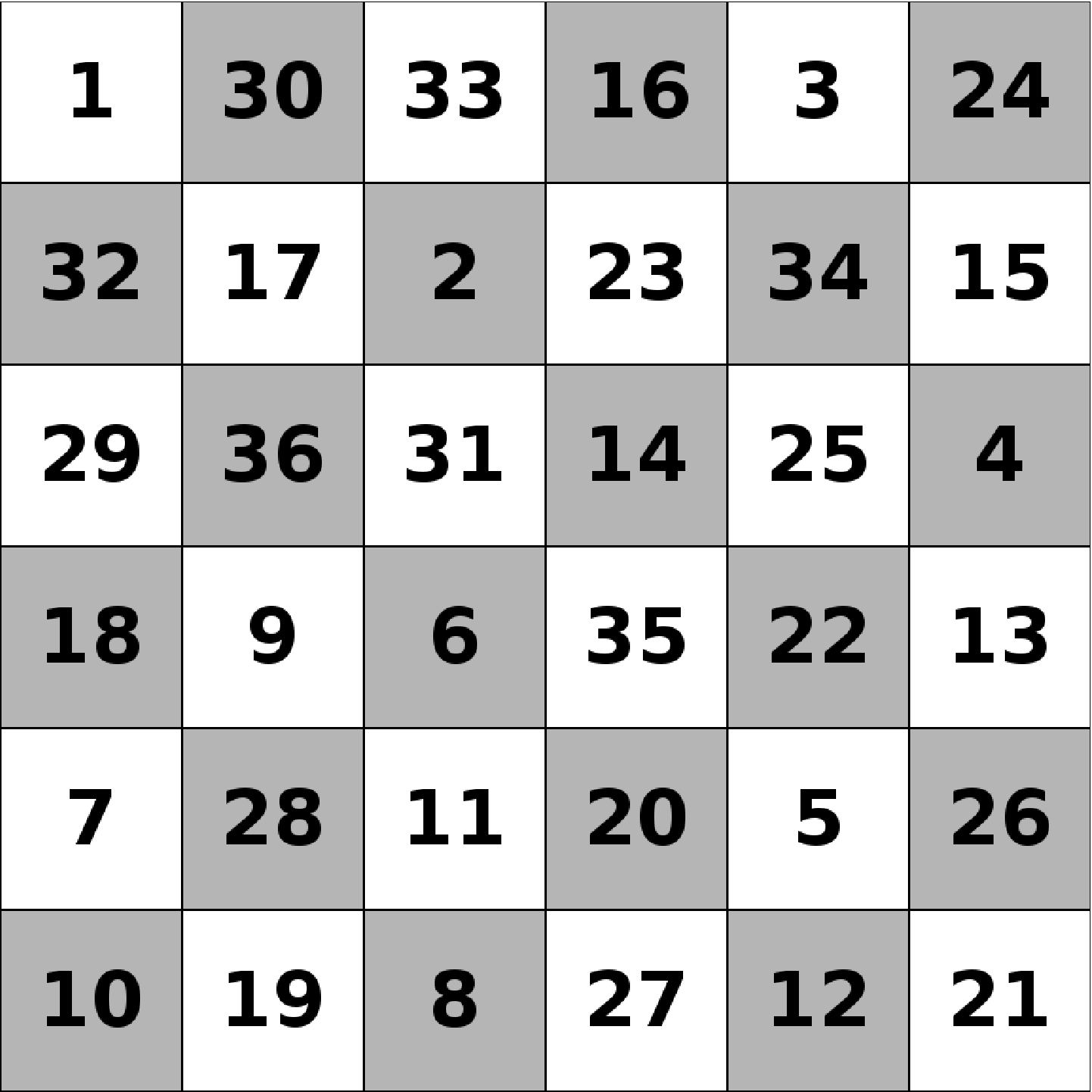
On a chessboard, a knight moves by two squares in one direction and by one square in the other one (like a L). A classical challenge is the so-called knight tour. The knight is placed on the empty board and, moving according to the rules of chess, must visit each square exactly once. A knight’s tour is called a closed tour if the knight ends on a square attacking the square from which it began. If the latter is not satisfied and the knight has visited each square exactly once, we call it an open tour.

Refer to caption — Figure 1. A $6\times 6$ closed tour

Some early solutions were given by Euler, see [Eul] and also by De Moivre (we refer to Mark R. Keen for historical remarks, see [Kee]). The problem was recently considered for various types of chessboards: as a cylinder [Wat1], a torus [Wat2], a sphere [Cai], the exterior of the cube [QiW], the interior of the cube [De], $\ldots$ It represents also an active field of research in computer science, e.g., [Pab] (see references therein). In this paper, we shall focus on rectangular boards.

In 1991, Schwenk considered the question of the closed knight tour problem in a $2$ -dimensional rectangular chessboard. He provided a necessary and sufficient condition on the size of the board in order to have a closed knight tour. He obtained:

Theorem 1.1 (Schwenk).

Let $1\leq m\leq n$ . The $m\times n$ chessboard has no closed knight tour if and only if one of the following assumption holds:

(a)

$m$ and $n$ are both odd,
(b)

$m\in\{1,2,4\}$ ,
(c)

$m=3$ and $n\in\{4,6,8\}$ .

We refer to [Sch] (see also [Wat]) for a proof. When conditions (a),(b), and (c) are not fulfilled, he reduced the problem to studying a finite number of elementary boards. On each of them, he exhibited a closed tour and then explained how to “glue” the elementary boards together, in order to make one closed tour for the union out of the disjoint ones given by the elementary blocks. We explain the latter on an example. Say we want a closed tour for a $12\times 6$ board. Write, side by side, two copies of Figure 1. Delete the connection between $21$ and $22$ for the left board and the connection between $28$ and $29$ for the right one. Then link $21$ with $28$ and $22$ with $29$ . The Hamiltonian cycle goes as follows:

	$\displaystyle 1[L]$	$\displaystyle\to 2[L]\to\ldots\to 21[L]\to 28[R]\to 27[R]\to\ldots\to 1[R]\to$
		$\displaystyle\to 36[R]\to\ldots\to 29[R]\to 22[L]\to 23[L]\to\dots\to 36[L]\to 1[L],$

where $[L]$ and $[R]$ stand for left and right, respectively.

We turn to the question for higher dimensions. In dimension $3$ or above, a knight moves by two steps along one coordinate and by one step along a different one. We refer to Section 2 for a mathematical definition. Stewart [Ste] and DeMaio [De] constructed some examples of $3$ -dimensional knight tours. Then, in 2011, in [DeM], DeMaio and Mathew extended Theorem 1.1 by classifying all the $3$ -dimensional rectangular chessboards which admit a knight tour.

Theorem 1.2 (DeMaio and Mathew).

Let $2\leq m\leq n\leq p$ . The $m\times n\times p$ chessboard has no closed knight tour if and only if one of the following assumption holds:

(a)

$m$ , $n$ , and $p$ are all odd,
(b)

$m=n=2$ ,
(c)

$m=2$ and $n=p=3$ .

The strategy is the same as in Theorem 1.1. We give an alternative proof of this result in Appendix A.2.

In this paper we extend the previous results to higher dimensional boards. We rely strongly on the structure of the solutions for the case $n=3$ to treat the case $n\geq 4$ . We proceed by induction. Before giving the main statement, we explain the key idea with Figure 1. We first extract two cross-patterns (cp). We represent them up to some rotation, see Figure 2. Note they are with disjoint support.

We construct a tour for a $6\times 6\times 2$ board first. We work with coordinates. The tour given in 1 is given by $(a^{i})_{i\in[\![1,36]\!]}$ , with $a^{1}:=(1,6)$ , $a^{2}:=(3,5)$ , $\ldots$ We take two copies of the tour given in 1 and denote them by $(a^{i},1)_{i\in[\![1,36]\!]}$ and $(a^{i},2)_{i\in[\![1,36]\!]}$ for the first and second copy, respectively. We can construct a tour as follows:

\displaystyle(3,2,1)\to(1,2,2)\to(3,3,2)\to\ldots\to(3,1,2)\to(1,1,1)\to\ldots\to(3,2,1).

We point out that we use coordinates in matrix way. To enhance the idea we rewrite it abusively by

\displaystyle(``36",1)\to(``30",2)\to(``31",2)\to\ldots\to(``29",2)\to(``1",1)\to\ldots\to(``36",1).

We explain how to treat a $6\times 6\times k$ board for $k\geq 3$ . As the proof is the same, we write the case $k=3$ . We use the two cp as follows:

	$\displaystyle(``36",1)$	$\displaystyle\to(``30",2)\to(``31",2)\to\ldots\to(``9",2)\to$
		$\displaystyle\to(``19",3)\to(``20",3)\to\ldots\to(``18",3)\to$
(1.1)			$\displaystyle\to(``10",2)\to(``11",2)\to\ldots\to(``29",2)\to$
		$\displaystyle\to(``1",1)\to\ldots\to(``36",1).$

Note that we have use only one cp on the first copy and one on last one. Two of them are still free. We can therefore repeat the procedure and add inductively further dimensions. For instance, we can go from a tour for a $6\times 6\times k$ board to one for a $6\times 6\times k\times l$ board, with $k,l\geq 2$ . One takes $l$ copies of the tour. By noticing that there are two cp on the initial tour, we proceed as in (1.1) for the tour. Thus, we will get a tour for the $6\times 6\times k\times l$ board, which contains in turn two cp. To prove all these facts, one can use coordinates. We refer to Section 3 for more details.

The strategy is now clear. We shall study the structure of the elementary boards, which are obtained in [DeM] and look for specific patterns into them. Then, we shall conclude by induction on the dimension. We obtain:

Theorem 1.3.

Let $2\leq n_{1}\leq n_{2}\leq...\leq n_{k}$ , with $k\geq 3$ . The $n_{1}\times\ldots\times n_{k}$ chessboard has no closed knight tour if and only if one of the following assumption holds:

(a)

For all $i$ , $n_{i}$ is odd,
(b)

$n_{k-1}=2$ ,
(c)

$n_{k}=3$ .

Note that the hypotheses are the same as the ones given in Theorem 1.2 when $k=3$ . In the same paper they asked about higher dimensional tours, This question was also asked by DeMaio [De] and Watkins [Wat3]. We mention that a conjecture for this theorem was given in [Kum].

The paper is organized as follows. In Section 2 we set the notation and define the graph structure induced by a knight on an $n$ dimensional board. Then, in Section 3 we introduce the notion of cross-patterns and explain how to use them in order to gain a dimension. In Section 4.1, we start the proof of Theorem 1.3 and provide all the negative answers. After that, in Section 4.3, we finish the proof of Theorem 1.3. In Section 5 we show we can apply this technique to the problem of knight’s tours with more general moves. Finally, in the appendix, we give an alternative proof of Theorem 1.2.

Acknowledgments: We would like to thank Imre Leader for useful discussions and comments on the script.

2. Notation

Let $\underline{n}:=(n_{1},\ldots,n_{k})$ be a multi-index where $n_{i}$ are with values in $\mathbb{N}\setminus\{0\}$ . We denote by $|\underline{n}|:=k$ , the size of the multi-index $\underline{n}$ . Set also $[\![a,b]\!]:=[a,b]\cap\mathbb{Z}$ . The chessboard associated to $\underline{n}$ is defined by

\mathcal{B}_{{\underline{n}}}:=[\![1,n_{1}]\!]\times\ldots\times[\![1,n_{|\underline{n}|}]\!].

We turn to the definition of the moves of the knight. We set:

	$\displaystyle\mathcal{C}_{\|{\underline{n}}\|}:=$	$\displaystyle\{(a_{1},\ldots,a_{\|\underline{n}\|})\in\mathbb{Z}^{\|{\underline{n}}\|},\quad\mbox{ such that }$
		$\displaystyle\hskip-14.22636pt\|\{i,a_{i}=0\}\|=\|{\underline{n}}\|-2,\quad\|\{i,a_{i}\in\{\pm 1\}\}\|=1,\quad\mbox{ and }\quad\|\{i,a_{i}\in\{\pm 2\}\}\|=1\}.$

We endow $\mathcal{B}_{{\underline{n}}}$ with a graph structure, as follows. We set $\mathcal{E}_{\underline{n}}:\mathcal{B}_{{\underline{n}}}\times\mathcal{B}_{{\underline{n}}}\to\{0,1\}$ be a symmetric function defined as follows:

(2.1)

\displaystyle\mathcal{E}_{\underline{n}}(a,b):=1,\quad\mbox{ if }\quad a-b:=(a_{1}-b_{1},\ldots,a_{|\underline{n}|}-b_{|\underline{n}|})\in\mathcal{C}_{|{\underline{n}}|}

and $0$ otherwise. In other words, $a$ is linked to $b$ by a knight move, if and only if $\mathcal{E}_{\underline{n}}(a,b):=1$ . The couple $\mathcal{G}_{\underline{n}}:=(\mathcal{B}_{\underline{n}},\mathcal{E}_{\underline{n}})$ is the non-oriented graph corresponding to all the possible paths of a knight on the chessboard associated to $\underline{n}$ .

Set $\phi:\mathcal{B}_{\underline{n}}\to\{-1,1\}$ given by $\phi(a_{1},\ldots,a_{|\underline{n}|}):=(-1)^{a_{1}\times\ldots\times a_{|\underline{n}|}}$ , i.e., we assign the color black or white to each square. Then note that given $a,b\in\mathcal{B}_{\underline{n}}$ such that $\mathcal{E}_{\underline{n}}(a,b)=1$ , one has $\phi(a)\times\phi(b)=-1$ . Therefore the graph $\mathcal{G}_{\underline{n}}:=(\mathcal{B}_{\underline{n}},\mathcal{E}_{\underline{n}})$ is bipartite.

Let $\{a^{i}\}_{i=1,\ldots,|\mathcal{B}_{\underline{n}}|}$ be some elements of $\mathcal{B}_{\underline{n}}$ . We say that $\{a^{i}\}_{i}$ is a Hamiltonian cycle if the elements are two by two distinct and if $\mathcal{E}_{\underline{n}}(a^{i},a^{i+1}):=1$ for all $i\in\{1,\ldots,|\mathcal{B}_{\underline{n}}|\}$ and if $\mathcal{E}_{\underline{n}}(a^{1},a^{|\mathcal{B}_{\underline{n}}|}):=1$ . Note that because of (2.1), $\mathcal{B}_{\underline{n}}$ has a closed knight tour is just rephrasing that fact that $\mathcal{G}_{\underline{n}}$ has a Hamiltonian cycle.

Remark 2.1.

Given a multi-index $\underline{n}$ and $\psi$ a bijection from $[\![1,|\underline{n}|]\!]$ onto itself, we set $\underline{m}$ of size $|\underline{n}|$ given by $m_{i}:=n_{\psi(i)}$ for all $i\in[\![1,|n|]\!]$ . Since $\mathcal{C}_{|\underline{n}|}=\mathcal{C}_{|\underline{m}|}$ is invariant under permutation, $\mathcal{G}_{\underline{n}}$ has a Hamiltonian cycle if and only $\mathcal{G}_{\underline{m}}$ has one.

3. Looking for patterns

In Proposition 3.7, see also Example 3.5 for $2$ -dimensional boards, we shall explain how to gain dimensions, for the question of closed tours, with the help of patterns.

Given an $n\times m$ board, we say that a pair of edges $((a_{1},b_{1}),(a_{2},b_{2}))$ and $((c_{1},d_{1}),(c_{2},d_{2}))$ in a tour is a site if

(|a_{1}-c_{1}|,|b_{1}-d_{1}|)=(|a_{2}-c_{2}|,|b_{2}-d_{2}|)\in\{(0,2),(2,0)\}

or if

(|a_{1}-c_{2}|,|b_{1}-d_{2}|)=(|a_{2}-c_{1}|,|b_{2}-d_{1}|)\in\{(0,2),(2,0)\}.

Roughly speaking, both endpoints of the two edges are two squares away from each other. The three possible configurations are given in Figure 3. The first will be cross-pattern and the two others parallel-patterns.

We generalize the definition for higher dimensional board. We denote by $(e_{i})_{i\in[\![1,d]\!]}$ the canonical basis of $\mathbb{R}^{d}$ .

Definition 3.1.

Given a Hamiltonian cycle $(a^{i})_{i\in I}$ for $\mathcal{G}_{\underline{n}}$ , we say that it contains the well-oriented parallel-pattern (wopp) if there are $c\in\mathcal{C}_{|{\underline{n}}|}$ , $n,m\in I$ , and $i\in[\![1,d]\!]$ so that:

	$\displaystyle a^{n+1}=a^{n}+c$	$\displaystyle\mbox{ and }a^{m}=a^{m+1}+c$
(3.1)		$\displaystyle a^{m}-a^{n+1}=a^{m+1}-a^{n}$	$\displaystyle\in\{\pm 2e_{i}\}.$

We denote this wopp by $(a^{n},a^{n+1},a^{m},a^{m+1})$ .

We say that it contains the non-well-oriented parallel-pattern (nwopp) if there are $c\in\mathcal{C}_{|{\underline{n}}|}$ , $n,m\in I$ , and $i\in[\![1,d]\!]$ so that:

	$\displaystyle a^{n+1}=a^{n}+c$	$\displaystyle\mbox{ and }a^{m+1}=a^{m}+c$
(3.2)		$\displaystyle a^{m}-a^{n}=a^{m+1}-a^{n+1}$	$\displaystyle\in\{\pm 2e_{i}\}$

We denote this nwocp by $(a^{n},a^{n+1},a^{m+1},a^{m})$ .

Note that the equality in (3.1) (resp. in (3.2)) is automatically satisfied by the condition with $c$ . We give an example in a $2$ -dimensional board in Figure 4.

We turn to cross-patterns. To each element $c:=(a_{1},\ldots,a_{\underline{n}})\in\mathcal{C}_{|{\underline{n}}|}$ , we associate two elements $e_{[c,1]}$ and $e_{[c,2]}$ of $\mathbb{Z}^{|{\underline{n}}|}$ , by setting

e_{[c,1]}(i):=\delta_{a_{i}\in\{\pm 1\}}\mbox{ and }e_{[c,2]}(i):=\delta_{a_{i}\in\{\pm 2\}},

where $\delta_{X}:=0$ if $X$ is empty and $\delta_{X}:=1$ otherwise. Note that:

c=\langle c,e_{[c,1]}\rangle e_{[c,1]}+\langle c,e_{[c,2]}\rangle e_{[c,2]}\in\{\pm 1e_{[c,1]}+\pm 2e_{[c,2]}\},

where $\langle\cdot,\cdot\rangle$ denotes the Euclidean scalar product in $\mathbb{R}^{|\underline{n}|}$ . We now flip $c$ with respect to $e_{[c,1]}$ . More precisely, we set

\tilde{c}:=-\langle c,e_{[c,1]}\rangle e_{[c,1]}+\langle c,e_{[c,2]}\rangle e_{[c,2]}.

Definition 3.2.

Given a Hamiltonian cycle $(a^{i})_{i\in I}$ for $\mathcal{G}_{\underline{n}}$ , we say that it contains the well-oriented cross-pattern (wocp) if there are $c\in\mathcal{C}_{|{\underline{n}}|}$ and $n,m\in I$ , so that:

(3.3)		$\displaystyle a^{n+1}=a^{n}+c$	$\displaystyle\mbox{ and }a^{m+1}=a^{m}+\tilde{c}$
	$\displaystyle a^{m}-a^{n}$	$\displaystyle=\langle c,e_{[c,1]}\rangle e_{[c,1]}.$

We denote this wocp by $(a^{n},a^{n+1},a^{m},a^{m+1})$ .

We say that it contains the non-well-oriented cross-pattern (nwocp) if there are $c\in\mathcal{C}_{|{\underline{n}}|}$ and $n,m\in I$ , so that:

(3.4)		$\displaystyle a^{n+1}=a^{n}+c$	$\displaystyle\mbox{ and }a^{m}=a^{m+1}+\tilde{c}$
	$\displaystyle a^{m+1}-a^{n}$	$\displaystyle=\langle c,e_{[c,1]}\rangle e_{[c,1]}.$

We denote this nwocp by $(a^{n},a^{n+1},a^{m+1},a^{m})$ .

Definition 3.3.

Given a Hamiltonian cycle $(a^{i})_{i\in I}$ , we say that $(a^{n},a^{n+1},a^{m},a^{m+1})$ is a well-oriented site (or pattern) if it is a wocp or a wopp. we say that $(a^{n},a^{n+1},a^{m+1},a^{m})$ is a non-well-oriented site (or pattern) if it is a nwocp or a nwopp.

The Properties (3.1) and (3.2) are important and we present the equivalent for cross-patterns. It would be extensively used in Example 3.5 and in the Proposition 3.7.

Remark 3.4.

In the case of the wocp (3.3), we have

a^{n+1}-a^{m}=a^{m+1}-a^{n}=\langle c,e_{[c,2]}\rangle e_{[c,2]}.

In particular, if $(a^{n},a^{n+1},a^{m+1},a^{m})$ is a well-oriented site, then there is an $i$ such that

a^{n+1}-a^{m}=\pm(a^{m+1}-a^{n})\in\{-2e_{i},2e_{i}\}.

In the case of the nwocp (3.4), we get

a^{n+1}-a^{m+1}=a^{m}-a^{n}=\langle c,e_{[c,2]}\rangle e_{[c,2]}.

This also yields that, if $(a^{n},a^{n+1},a^{m+1},a^{m})$ is a non-well-oriented site, then there is an $i$ such that

a^{n+1}-a^{m+1}=\pm(a^{m}-a^{n})\in\{-2e_{i},2e_{i}\}.

We now explain how to connect two Hamiltonian cycles and gain one dimension with the help of sites. We mention that, in the $2$ -dimensional case, the existence of sites will be discussed in Proposition 4.2.

Example 3.5.

Take $\mathcal{G}_{\underline{n}}$ , with $|\underline{n}|=2$ , such that it contains a Hamiltonian cycle $(a^{i})_{i\in I}$ , see Theorem 1.1. Take now $\underline{m}:=(\underline{n},2)$ . Note that $\mathcal{G}_{\underline{m}}$ contains two cycles:

(a^{i},1)_{i\in I}\mbox{ and }(a^{i},2)_{i\in I}.

Suppose there is a well-oriented site $(a^{n},a^{n+1},a^{m},a^{m+1})$ . Using Remark (3.4), we obtain immediately that $\mathcal{E}_{\underline{m}}((a^{n},1),(a^{m+1},2))=1$ and $\mathcal{E}_{\underline{m}}((a^{m},2),(a^{n+1},1))=1$ . We can construct a Hamiltonian cycle as follows:

\displaystyle(a^{n},1)\to(a^{m+1},2)\to(a^{m+2},2)\to\ldots\to(a^{m},2)\to(a^{n+1},1)\to\ldots\to(a^{n},1).

Suppose now there is a non-well-oriented site $(a^{n},a^{n+1},a^{m+1},a^{m})$ . Similarly, We construct a Hamiltonian cycle as follows:

\displaystyle(a^{n},1)\to(a^{m},2)\to(a^{m-1},2)\to\ldots\to(a^{m+1},2)\to(a^{n+1},1)\to\ldots\to(a^{n},1).

Note that we went backward on the second copy.

It is obvious that one can gain as many dimension as one has disjoint cross-patterns. However, the situation is much better: having solely two of them are enough to gain as many dimension as we want.

Definition 3.6.

A tour would be called bi-sited if it contains two sites with disjoint support, i.e., such that the endpoints of the four pair of edges are two by two disjoint.

We rely on the next Proposition.

Proposition 3.7.

Take $\mathcal{G}_{\underline{n}}$ . Suppose that it contains a bi-sited Hamiltonian cycle. Take now $\underline{m}:=(\underline{n},k)$ , with $k\geq 2$ . Then $\mathcal{G}_{\underline{m}}$ contains a bi-sited Hamiltonian cycle.

Proof.

As the demonstration is similar, we shall present only the case of two well-oriented sites. Set $(a^{i})_{i\in I}$ the Hamiltonian cycle. Note that $(a^{i},j)_{i\in I}$ , for $j\in[\![1,k]\!]$ , are $k$ disjoint cycle in $\mathcal{G}_{\underline{m}}$ . Take two well-oriented sites $(a^{n_{1}},a^{n_{1}+1},a^{m_{1}},a^{m_{1}+1})$ and $(a^{n_{2}},a^{n_{2}+1},a^{m_{2}},a^{m_{2}+1})$ . Let $k$ be even. Using Remark 3.4, we obtain

	$\displaystyle(a^{n_{1}},1)$	$\displaystyle\to(a^{m_{1}+1},2)\to(a^{m_{1}+2},2)\to\ldots\to(a^{n_{2}},2)\to$
		$\displaystyle\to(a^{m_{2}+1},3)\to(a^{m_{2}+2},3)\to\ldots\to(a^{n_{1}},3)\to$
		$\displaystyle\to(a^{m_{1}+1},4)\to(a^{m_{1}+2},4)\to\ldots\to(a^{n_{2}},4)\to\ldots$
(3.5)			$\displaystyle\to(a^{m_{2}+1},k-1)\to(a^{m_{2}+2},k-1)\to\ldots\to(a^{n_{1}},k-1)\to$
(3.6)			$\displaystyle\to(a^{m_{1}+1},k)\to(a^{m_{1}+2},k)\to\ldots\to(a^{m_{1}},k)\to$
(3.7)			$\displaystyle\to(a^{n_{1}+1},k-1)\to(a^{n_{1}+2},k-1)\to\ldots\to(a^{m_{2}},k-1)\to\ldots$
		$\displaystyle\to(a^{n_{2}+1},2)\to(a^{n_{2}+2},2)\to\ldots\to(a^{m_{1}},2)$
		$\displaystyle\to(a^{n_{1}+1},1)\to(a^{n_{1}+2},1)\to\ldots\to(a^{n_{1}},1).$

Finally note that $((a^{n_{2}},j),(a^{n_{2}+1},j),(a^{m_{2}},j),(a^{m_{2}+1},j))$ with $j\in\{1,k\}$ are well-oriented sites for this Hamiltonian cycle in $\mathcal{G}_{\underline{m}}$ . When $k$ is odd, we replace the lines (3.5), (3.6), and (3.7) by

		$\displaystyle\to(a^{m_{1}+1},k-1)\to(a^{m_{1}+2},k-1)\to\ldots\to(a^{n_{2}},k-1)\to$
		$\displaystyle\to(a^{m_{2}+1},k)\to(a^{m_{2}+2},k)\to\ldots\to(a^{m_{2}},k)\to$
		$\displaystyle\to(a^{n_{2}+1},k-1)\to(a^{n_{2}+2},k-1)\to\ldots\to(a^{m_{1}},k-1)\to\ldots$

In this case, we get $((a^{n_{2}},1),(a^{n_{2}+1},1),(a^{m_{2}},1),(a^{m_{2}+1},1))$ and $((a^{n_{1}},k),(a^{n_{1}+1},k),(a^{m_{1}},k),(a^{m_{1}+1},k))$ are well-oriented sites associated to the Hamiltonian cycle in $\mathcal{G}_{\underline{m}}$ . ∎

4. Into the proof

In this section we give the proof of Theorem 1.3 and consider boards associated to a multi-index $\underline{n}:=(n_{1},\ldots,n_{|\underline{n}|})$ , where $n_{i}\geq 2$ and $|\underline{n}|\geq 3$ .

4.1. Forbidden boards

We start with the sufficient part of Theorem 1.3. It is a straightforward generalization of the dimension $3$ . There are three main cases:

a) $n_{i}\in(2\mathbb{N}+1)$ , for all $i$ . A bipartite graph cannot have a Hamiltonian cycle if its cardinality is odd.

b) $\underline{n}:=(2,2,\ldots,2,k)$ , with $k\geq 2$ . Set $a^{0}:=(2,2,\ldots,2)\in\mathcal{B}_{n}$ . Let $(a^{i})_{i\geq 0}$ , be the elements of a Hamiltonian cycle. Note that $(a^{0}-a^{i})\in(\{1,2\},\ldots,\{1,2\},2\mathbb{Z})$ , for all $i\geq 0$ . Then, $(1,1,\ldots,1)$ is never reached. Contradiction.

c) $\underline{n}:=(n_{1},\ldots,n_{|\underline{n}|})$ , with $2\leq n_{1}\leq\ldots\leq n_{|\underline{n}|}\leq 3$ . Set $a:=(2,\ldots,2)\in\mathcal{B}_{n}$ and note that there is no $b\in\mathcal{C}_{|\underline{n}|}$ , such that $a+b\in\mathcal{B}_{\underline{n}}$ . Therefore, the graph $\mathcal{G}_{\underline{n}}:=(\mathcal{B}_{\underline{n}},\mathcal{E}_{\underline{n}})$ has no closed tour.

Remark 4.1.

Note that the two last cases correspond to disconnected boards.

4.2. Bi-sited boards in dimension $2$ and $3$

We start by the existence in dimension $2$ .

Proposition 4.2.

Every closed tour on an $n\times m$ board is bi-sited.

Proof.

First, there is no closed tour on a $2\times k$ and on $4\times k$ boards.

i) Case ${\bf 3\times k}$ , for ${\bf k\geq 10}$ : Note that $k$ is even. First one has $(1,1)$ which is linked to $(3,2)$ and to $(2,3)$ . The possible neighbors of $(1,3)$ are $(3,2)$ , $(2,1)$ , $(3,4)$ , $(2,5)$ . As we have a cycle, exactly two of them are linked to $(1,3)$ and three of them are part of a pattern (the second one forms a cross-pattern and the two last one parallel patterns). Then, there is at least one site. Secondly we repeat the argument for the upper right corner and get a new site. Since $k\geq 10$ , the two sites are with disjoint supports.

ii) Case ${\bf k\times l}$ , for ${\bf k\geq 5,}$ and ${\bf l\geq 6}$ : We flip the board and consider $l\times k$ . We repeat twice the first part of the point i) for the sub-board of size $3\times k$ that contains the upper left corner and for the one that contains the lower left corner. We get two disjoint sites. ∎

This proposition will be very useful in Appendix A.2. Indeed, combining it with Proposition 3.7, we infer:

Corollary 4.3.

If an $n\times m$ closed tour exists then so does an $n\times m\times p_{1}....\times p_{r}$ closed tour for any $p_{1},\ldots,p_{r}\in\mathbb{N}\setminus\{0\}$ .

We were not able to obtain an analogue to Proposition 4.2 for $3$ dimensional boards. However, for our purpose it is enough to prove the existence of specific bi-sited tours. In this section we will rely on the construction of [DeM] and in Appendix A.2, we will give a self-contained proof.

Theorem 4.4.

Let $2\leq m\leq n\leq p$ . The $m\times n\times p$ chessboard has a bi-sited closed tour if and only if one of the following assumption holds:

(a)

$m$ , $n$ , or $p$ is even,
(b)

$n\geq 3$ ,
(c)

$p\geq 4$ .

Proof.

Without going into details, we give a rough idea about the approach of [DeM]. Take $n\times m\times p$ , that is not satisfying the hypotheses a), b) and c) of Theorem 1.2. Note that at least one of them is even (say $n$ ). Subsequently, one basically works modulus $4$ : An $n\times m\times p$ block can be written as a union of the following ones: $2\times 4\times 4$ , $2\times 4\times 5$ , $2\times 4\times 6$ , $2\times 4\times 3$ , $2\times 5\times 5$ , $2\times 5\times 6$ , $2\times 5\times 3$ , $2\times 6\times 6$ , $2\times 6\times 3$ , $2\times 7\times 3$ , $4\times 3\times 3$ , $6\times 3\times 3$ . The list is rather long since one has no Hamiltonian cycle for $2\times 2\times 3$ and $2\times 3\times 3$ boards. Then, the authors construct some Hamiltonian cycle for each elementary blocks. After that, given two compatible blocks, by deleting one edge from each block and by creating two edges that are “gluing” these blocks together, they construct a Hamiltonian cycle for the union, starting with the two disjoint ones.

First, we study the elementary blocks that are exhibited in [DeM]. For each of them, we give the list of well-oriented cross-patterns (wocp), non-well-oriented cross-patterns (nwocp) and also the edges that are used to combine two different blocks, in order to create a Hamiltonian cycle for the union. We will not exhibit parallel-patterns. For the latter, we indicate the other figure that is glued with and denote it between square brackets. We also strike out all the wocp and nwocp which are incompatible with the gluing operation of [DeM]. For instance, in Figure $6$ , we struck $(2,3,21,20)$ out, because the edge $(20,21)$ is already used when one glues Figure $35$ .

\displaystyle\begin{array}[]{c}\begin{array}[]{|c|c|c|}\hline\cr\mbox{Wocp}&\mbox{Nwocp}&\mbox{Used edges [with Figure]}\\ \hline\cr(4,5,11,12)&(1,2,22,21)&(3,4)[6,11,14,17],(8,9)[6]\\ (7,8,28,29)&\makebox[0.0pt][l]{\hbox{$(2,3,21,20)$}}\rule[3.75pt]{51.11113pt}{0.5pt}&(10,11)[6],(14,15)[6],\\ &(13,14,18,17)&(20,21)[35],(25,26)[6],\\ &&(27,28)[6]\\ \hline\cr\end{array}\\ \\ \mbox{Case of the Figure }6:\mbox{ size }2\times 4\times 4\end{array}

\displaystyle\begin{array}[]{c}\begin{array}[]{|c|c|c|}\hline\cr\mbox{Wocp}&\mbox{Nwocp}&\mbox{Used edges [with Figure]}\\ \hline\cr(1,2,30,31)&(14,15,35,34)&(4,5)[20],(8,9)[20],\\ \makebox[0.0pt][l]{\hbox{$(4,5,31,32)$}}\rule[3.75pt]{51.11113pt}{0.5pt}&\makebox[0.0pt][l]{\hbox{$(16,17,23,22)$}}\rule[3.75pt]{61.11116pt}{0.5pt}&(10,11)[11],(11,12)[23],\\ \makebox[0.0pt][l]{\hbox{$(12,13,39,40)$}}\rule[3.75pt]{61.11116pt}{0.5pt}&&(16,17)[11],(17,18)[26],\\ (19,20,24,25)&&(31,32)[11],(37,38)[11],(39,40)[6]\\ \hline\cr\end{array}\\ \\ \mbox{Case of the Figure }11:\mbox{ size }2\times 4\times 5\end{array}

\displaystyle\begin{array}[]{c}\begin{array}[]{|c|c|c|}\hline\cr\mbox{Wocp}&\mbox{Nwocp}&\mbox{Used edges [with Figure]}\\ \hline\cr(1,2,3,4)&(14,15,47,46)&(4,5)[29],(9,10)[32],\\ (7,8,26,27)&&(28,29)[14],(29,30)[14],\\ (8,9,25,26)&&(30,31)[14],(36,37)[6],\\ (10,11,31,32)&&(39,40)[14],(43,44)[29],\\ (11,12,44,45)&&(47,48)[23]\\ (13,14,32,33)&&\\ (15,16,34,35)&&\\ \makebox[0.0pt][l]{\hbox{$(18,19,39,40)$}}\rule[3.75pt]{61.11116pt}{0.5pt}&&\\ (48,1,37,38)&&\\ \hline\cr\end{array}\\ \\ \mbox{Case of the Figure }14:\mbox{ size }2\times 4\times 6\end{array}

\displaystyle\begin{array}[]{c}\begin{array}[]{|c|c|c|}\hline\cr\mbox{Wocp}&\mbox{Nwocp}&\mbox{Used edges [with Figure]}\\ \hline\cr(8,9,21,22)&(2,3,7,6)&(4,5)[17],(5,6)[17],\\ (9,10,16,17)&&(7,8)[17],(11,12)[6],\\ (10,11,15,16)&&(20,21)[17,26,32,35]\\ \hline\cr\end{array}\\ \\ \mbox{Case of the Figure }17:\mbox{ size }2\times 4\times 3\end{array}

\displaystyle\begin{array}[]{c}\begin{array}[]{|c|c|c|}\hline\cr\mbox{Wocp}&\mbox{Nwocp}&\mbox{Used edges [with Figure]}\\ \hline\cr(3,4,38,39)&(9,10,24,23)&(20,21)[11],(43,44)[20],\\ (5,6,28,29)&(18,19,33,32)&(47,48)[11],(49,50)[20]\\ (8,9,25,26)&\makebox[0.0pt][l]{\hbox{$(19,20,50,49)$}}\rule[3.75pt]{61.11116pt}{0.5pt}&\\ (12,13,45,46)&\makebox[0.0pt][l]{\hbox{$(20,21,43,42)$}}\rule[3.75pt]{61.11116pt}{0.5pt}&\\ \makebox[0.0pt][l]{\hbox{$(14,15,47,48)$}}\rule[3.75pt]{61.11116pt}{0.5pt}&&\\ (17,18,30,31)&&\\ \hline\cr\end{array}\\ \\ \mbox{Case of the Figure }20:\mbox{ size }2\times 5\times 5\end{array}

One has to be careful with the block $2\times 5\times 6$ which is given in Figure $23$ of [DeM]. Indeed, one sees that $1$ cannot be reached from $60$ , therefore this is not a Hamiltonian cycle but just a path. To fix this, we propose to take:

We replace the table following the board, i.e., the table on the top of page $9$ . By

	Delete edges	Create edges
Vertical	$11-12$ top board, $12-13$ bottom board	$11-12$ , $12-13$
Horizontal	$32-33$ left board, $47-48$ right board	$32-47$ , $33-48$
Front	$1-2$ front board, $44-45$ back board	$1-44$ , $2-45$

This yields:

\displaystyle\begin{array}[]{c}\begin{array}[]{|c|c|c|}\hline\cr\mbox{Wocp}&\mbox{Nwocp}&\mbox{Used edges [with Figure]}\\ \hline\cr(6,7,53,54)&(3,4,52,51)&(1,2)[23],(12,13)[11],\\ (13,14,30,31)&(10,11,29,28)&(32,33)[14],(44,45)[23]\\ &(16,17,23,22)&\\ &(18,19,35,34)&\\ &(19,20,36,35)&\\ &(20,21,37,36)&\\ &(39,40,46,45)&\\ &(41,42,58,57)&\\ &(42,43,59,58)&\\ &(43,44,60,59)&\\ \hline\cr\end{array}\\ \\ \mbox{Case of the new Figure }23:\mbox{ size }2\times 5\times 6\end{array}

\displaystyle\begin{array}[]{c}\begin{array}[]{|c|c|c|}\hline\cr\mbox{Wocp}&\mbox{Nwocp}&\mbox{Used edges [with Figure]}\\ \hline\cr\makebox[0.0pt][l]{\hbox{$(6,7,23,24)$}}\rule[3.75pt]{51.11113pt}{0.5pt}&(3,4,22,21)&(14,15)[11],(23,24)[17],\\ &(9,10,16,15)&(27,28)[26],(29,30)[26]\\ &\makebox[0.0pt][l]{\hbox{$(11,12,28,27)$}}\rule[3.75pt]{61.11116pt}{0.5pt}&\\ &(12,13,29,28)&\\ &\makebox[0.0pt][l]{\hbox{$(13,14,30,29)$}}\rule[3.75pt]{61.11116pt}{0.5pt}&\\ \hline\cr\end{array}\\ \\ \mbox{Case of the Figure }26:\mbox{ size }2\times 5\times 3\end{array}

\displaystyle\begin{array}[]{c}\begin{array}[]{|c|c|c|}\hline\cr\mbox{Wocp}&\mbox{Nwocp}&\mbox{Used edges [with Figure]}\\ \hline\cr\makebox[0.0pt][l]{\hbox{$(15,16,62,63)$}}\rule[3.75pt]{61.11116pt}{0.5pt}&(2,3,69,68)&(15,16)[14],(22,23)[29],\\ (16,17,57,58)&(4,5,47,46)&(29,30)[14],(32,33)[29]\\ (47,48,72,1)&(6,7,37,36)&\\ &(7,8,36,35)&\\ &(10,11,51,50)&\\ &(12,13,39,38)&\\ &(20,21,53,52)&\\ &(23,24,70,69)&\\ &(27,28,64,63)&\\ &(30,31,43,42)&\\ &(31,32,42,41)&\\ \hline\cr\end{array}\\ \\ \mbox{Case of the Figure }29:\mbox{ size }2\times 6\times 6\end{array}

\displaystyle\begin{array}[]{c}\begin{array}[]{|c|c|c|}\hline\cr\mbox{Wocp}&\mbox{Nwocp}&\mbox{Used edges [with Figure]}\\ \hline\cr(6,7,15,16)&(3,4,14,13)&(11,12)[14],(18,19)[32],\\ (8,9,17,18)&(4,5,15,14)&(22,23)[32],(26,27)[17]\\ \makebox[0.0pt][l]{\hbox{$(18,19,31,32)$}}\rule[3.75pt]{61.11116pt}{0.5pt}&(25,26,34,33)&\\ (19,20,28,29)&\makebox[0.0pt][l]{\hbox{$(26,27,35,34)$}}\rule[3.75pt]{61.11116pt}{0.5pt}&\\ \hline\cr\end{array}\\ \\ \mbox{Case of the Figure }32:\mbox{ size }2\times 6\times 3\end{array}

\displaystyle\begin{array}[]{c}\begin{array}[]{|c|c|c|}\hline\cr\mbox{Wocp}&\mbox{Nwocp}&\mbox{Used edges [with Figure]}\\ \hline\cr(2,3,25,26)&(3,4,24,23)&(7,8)[6],(12,13)[35],\\ (6,7,19,20)&(5,6,22,21)&(13,14)[17],(14,15)[35]\\ \makebox[0.0pt][l]{\hbox{$(7,8,16,17)$}}\rule[3.75pt]{51.11113pt}{0.5pt}&(32,33,39,38)&\\ (8,9,15,16)&(33,34,40,39)&\\ \makebox[0.0pt][l]{\hbox{$(13,14,37,38)$}}\rule[3.75pt]{61.11116pt}{0.5pt}&&\\ \hline\cr\end{array}\\ \\ \mbox{Case of the Figure }35:\mbox{ size }2\times 7\times 3\end{array}

\displaystyle\begin{array}[]{c}\begin{array}[]{|c|c|c|}\hline\cr\mbox{Wocp}&\mbox{Nwocp}&\mbox{Used edges [with Figure]}\\ \hline\cr&(3,4,36,35)&(9,10)[39],(28,29)[39]\\ &\makebox[0.0pt][l]{\hbox{$(9,10,20,19)$}}\rule[3.75pt]{56.11115pt}{0.5pt}&\\ &(11,12,16,15)&\\ &\makebox[0.0pt][l]{\hbox{$(28,29,1,36)$}}\rule[3.75pt]{56.11115pt}{0.5pt}&\\ \hline\cr\end{array}\\ \\ \mbox{Case of the Figure }39:\mbox{ size }4\times 3\times 3\end{array}

\displaystyle\begin{array}[]{c}\begin{array}[]{|c|c|c|}\hline\cr\mbox{Wocp}&\mbox{Nwocp}&\mbox{Used edges [with Figure]}\\ \hline\cr(2,3,5,6)&(4,5,9,8)&(21,22)[40],(28,29)[40]\\ (10,11,15,16)&\makebox[0.0pt][l]{\hbox{$(18,19,29,28)$}}\rule[3.75pt]{61.11116pt}{0.5pt}&\\ (11,12,14,15)&(32,33,43,42)&\\ (13,14,16,17)&&\\ (19,20,22,23)&&\\ (20,21,25,26)&&\\ \makebox[0.0pt][l]{\hbox{$(21,22,24,25)$}}\rule[3.75pt]{61.11116pt}{0.5pt}&&\\ (36,37,49,50)&&\\ \hline\cr\end{array}\\ \\ \mbox{Case of the Figure }40:\mbox{ size }6\times 3\times 3\end{array}

In every case there is at least a pair cross-patterns which have disjoint supports. Now thanks to the proof of Theorem 1.2, we get there is a Hamiltonian cycle in $\mathcal{G}_{\underline{n}}$ which is obtained by gluing together Hamiltonian cycles coming from the elementary blocks that we have just discussed. Therefore, the Hamiltonian cycle is bi-sited.∎

4.3. Main result

We finish the proof of Theorem 1.3.

Proof of Theorem 1.3.

The sufficient part was proved in Section 4.1. We deal with the necessary part by an induction on:

$\mathcal{P}_{k}:=$ “Given a multi-index $\underline{n}=(n_{1},n_{2},\ldots,n_{k})$ , where $2\leq n_{1}\leq n_{2}\leq\ldots\leq n_{k}$ and such that:

(a)

There is $i_{0}\in[\![1,k]\!]$ such that $n_{i_{0}}$ is even,
(b)

$n_{k-1}\geq 3$ ,
(c)

$n_{k}\geq 4$ ,

then, $\mathcal{G}_{\underline{n}}$ contains a bi-sited Hamiltonian cycle.”

for all $k\geq 3$ .

Basis: Theorem 4.4 yields $\mathcal{P}_{3}$ .

Inductive step: Suppose that $\mathcal{P}_{k}$ holds true for some $k\geq 3$ . Take $\underline{n}=(n_{1},n_{2},\ldots,n_{\bf k+1})$ , where $2\leq n_{1}\leq n_{2}\leq\ldots\leq n_{k+1}$ , such that a), b) and c) hold true.

If all $n_{i}$ but one are odd, then, up to a permutation, we can always suppose that $n_{1}$ is odd. We set

(4.1)

\displaystyle\underline{n^{\prime}}=(n_{2},\ldots,n_{k+1}).

Otherwise, without operating a permutation, we set (4.1).

Note that $\mathcal{G}_{\underline{n}^{\prime}}$ satisfies the hypothesis a), b) and c) of $\mathcal{P}_{k}$ and therefore, by $\mathcal{P}_{k}$ , we get it contains a Hamiltonian cycle with at least well-oriented or two disjoint non-well-oriented cross-patterns. We apply Proposition 3.7 and get $\mathcal{P}_{k+1}$ is true.

Therefore, we have proved by induction that $\mathcal{P}_{k}$ is true for all $k\geq 3$ . In particular, this proves the theorem. ∎

Using Remark 4.1, we derive:

Corollary 4.5.

For $k\geq 3$ and $n_{i}\geq 2$ . Set $\underline{n}:=(n_{1},\ldots,n_{k})$ . Suppose that some $n_{i}$ is even. Then, a closed tour exists on $\mathcal{B}_{\underline{n}}$ if and only if $\mathcal{G}_{\underline{n}}$ is connected.

5. Generalised knight’s tours on a chessboard

The knight’s tour is a specific case of many general questions. A natural one to ask would be, what about more general moves? For example instead of the knight being able to move $(\pm 1,\pm 2)$ or $(\pm 2,\pm 1)$ what if the knight could move $(\pm\alpha,\pm\beta)$ or $(\pm\beta,\pm\alpha)$ ?

Given a chessboard $\mathcal{B}_{{\underline{n}}}$ and $\alpha,\beta\in\mathbb{N}\setminus\{0\}$ we define as before

	$\displaystyle\mathcal{C}^{\alpha,\beta}_{\|{\underline{n}}\|}:=$	$\displaystyle\{(a_{1},\ldots,a_{\|\underline{n}\|})\in\mathbb{Z}^{\|{\underline{n}}\|},\quad\mbox{ such that }$
		$\displaystyle\hskip-14.22636pt\|\{i,a_{i}=0\}\|=\|{\underline{n}}\|-2,\quad\|\{i,a_{i}\in\{\pm\alpha\}\}\|=1,\quad\mbox{ and }\quad\|\{i,a_{i}\in\{\pm\beta\}\}\|=1\}.$

and we endow $\mathcal{B}_{{\underline{n}}}$ with a graph structure, as follows. We set $\mathcal{E}^{\alpha,\beta}_{\underline{n}}:\mathcal{B}_{{\underline{n}}}\times\mathcal{B}_{{\underline{n}}}\to\{0,1\}$ to be the symmetric function defined as follows:

\displaystyle\mathcal{E}^{\alpha,\beta}_{\underline{n}}(a,b):=1,\quad\mbox{ if }\quad a-b:=(a_{1}-b_{1},\ldots,a_{|\underline{n}|}-b_{|\underline{n}|})\in\mathcal{C}^{\alpha,\beta}_{|{\underline{n}}|}

and $0$ otherwise. The couple $\mathcal{G}^{\alpha,\beta}_{\underline{n}}:=(\mathcal{B}_{\underline{n}},\mathcal{E}^{\alpha,\beta}_{\underline{n}})$ is the graph corresponding to all the possible paths of a generalised knight on the chessboard associated to $\underline{n}$ . Note that it is bipartite. We define an $(\alpha,\beta)$ -tour on $\mathcal{B}_{\underline{n}}$ to be a Hamiltonian cycle on $\mathcal{G}^{\alpha,\beta}_{\underline{n}}$ .

Knuth showed in [Knu] that in $2$ dimensions if $\alpha\geq\beta$ then $\mathcal{G}^{\alpha,\beta}_{(n_{1},n_{2})}$ is connected if and only if $\gcd(\alpha+\beta,\alpha-\beta)=1$ , $n_{1}\geq 2\alpha$ , and $n_{2}\geq\alpha+\beta$ .

Remark 5.1.

If an $(\alpha,\beta)$ -tour of $\mathcal{B}_{{\underline{n}}}$ exists then $\alpha$ and $\beta$ must be coprime. Indeed, $(1,1,\ldots,1)$ is connected to $(2,1,1\ldots,1)$ . Therefore, there are $k,l\in\mathbb{Z}$ such that $k\alpha+l\beta=1$ .

We extend the concept of sites to this setting and recall that $(e_{j})_{j\in[\![1,n]\!]}$ denotes the canonical basis of $\mathbb{R}^{n}$ .

Definition 5.2.

Given an $(\alpha,\beta)$ -tour $(a^{i})_{i\in I}$ , we say that it contains a well-oriented $\alpha$ -site if there are $n,m\in I$ and $j\in[\![1,n]\!]$ , such that

a^{n+1}-a^{m}=\pm(a^{m+1}-a^{n})\in\{-\alpha e_{j},\alpha e_{j}\}.

We denote it by $(a^{n},a^{n+1},a^{m},a^{m+1})$ .

Moreoever, we say that it contains a non-well-oriented $\alpha$ -site if there are $n,m\in I$ and $j\in[\![1,n]\!]$ , such that

a^{n}-a^{m}=\pm(a^{m+1}-a^{n+1})\in\{-\alpha e_{j},\alpha e_{j}\}.

We denote it by $(a^{n},a^{n+1},a^{m+1},a^{m})$ . We define similarly $\beta$ -sites.

As in Section 3 we can use $\alpha$ -sites and $\beta$ -sites to join together two cycles. The difference is that it connects two copies which are $\beta$ ( $\alpha$ resp.) far from one another.

Example 5.3.

More concretely, given an Hamiltonian $(a^{i})_{i\in I}$ on $\mathcal{G}^{\alpha,\beta}_{\underline{n}}$ that contains a well-oriented $\alpha$ -site $(a^{n},a^{n+1},a^{m},a^{m+1})$ , let ${\underline{m}}:=({\underline{n}},\beta+1)$ so that $\mathcal{B}_{\underline{m}}=(\mathcal{B}_{\underline{n}},1)\times(\mathcal{B}_{\underline{n}},2)\times\ldots\times(\mathcal{B}_{\underline{n}},\beta+1)$ . Noting that $\mathcal{G}_{{\underline{m}}}^{\alpha,\beta}$ contains the two cycles, $(a^{i},1)_{i\in I}$ and $(a^{i},\beta+1)_{i\in I}$ , we see that

	$\displaystyle(a^{n},1)$	$\displaystyle\to(a^{m+1},\beta+1)\to(a^{m+2},\beta+1)\to\ldots\to(a^{m},\beta+1)\to$
		$\displaystyle\to(a^{n+1},1)\to(a^{n+2},1)\to\ldots\to(a^{n},1)$

is a cycle on $(\mathcal{B}_{\underline{n}},1)\cup(\mathcal{B}_{\underline{n}},\beta+1)$ . The case for a non-well-oriented site is similar except that we reverse the orientation of the $(\beta+1)$ -th copy.

We first prove an analogue of Proposition 3.7 for $(\alpha,\beta)$ -sites.

Proposition 5.4.

Suppose that $\mathcal{G}^{\alpha,\beta}_{\underline{n}}$ contains a Hamiltonian cycle which contains $2$ $\alpha$ -sites and $2$ $\beta$ -sites, which are two by two disjoint. Take now $\underline{m}:=(\underline{n},k)$ , with $k\geq\alpha+\beta-1$ . Then $\mathcal{G}^{\alpha,\beta}_{\underline{m}}$ contains a Hamiltonian cycle which contains $2$ $\alpha$ -sites and $2$ $\beta$ -sites, which are two by two disjoint.

Proof.

Recall that by Remark 5.1 $\alpha$ and $\beta$ are coprime. Set $\alpha>\beta$ . As the demonstration is similar, we shall present only the case where all $4$ sites are well-oriented. Let $(a^{i})_{i\in I}$ be the Hamiltonian cycle. Note that $(a^{i},j)_{i\in I}$ , for $j\in[\![1,k]\!]$ , are $k$ disjoint cycles in $\mathcal{G}^{\alpha,\beta}_{\underline{m}}$ .

We start with the two $\alpha$ -sites $(a^{n_{1}},a^{n_{1}+1},a^{m_{1}},a^{m_{1}+1})$ and $(a^{n_{2}},a^{n_{2}+1},a^{m_{2}},a^{m_{2}+1})$ in $(a^{i})_{i\in I}$ . As in Proposition 3.7 and in the spirit of Example 5.3, for all $i\in[\![1,\beta]\!]$ , we connect the $i$ -th layer to the $i+\beta$ -th layer with the help of the first $\alpha$ -site, then the $i+2\beta$ -th layer with the help of the second $\alpha$ -site $\ldots$ until we have a cycle on

\mathcal{T}_{i}:=\bigcup_{c\in\big[\!\!\big[0,\lfloor\frac{k-i}{\beta}\rfloor\beta\big]\!\!\big]}(\mathcal{B}_{{\underline{n}}},\beta c+i),

for all $i\in[\![1,\beta]\!]$ . Note that $\cup_{i\in[\![1,\beta]\!]}\mathcal{T}_{i}$ is a partition of $\mathcal{B}_{\underline{m}}$ . More concretely, for the first layer and when $\lfloor\frac{k-1}{\beta}\rfloor$ is even, this gives:

	$\displaystyle(a^{n_{1}},1)$	$\displaystyle\to(a^{m_{1}+1},\beta+1)\to(a^{m_{1}+2},\beta+1)\to\ldots\to(a^{n_{2}},\beta+1)\to$
		$\displaystyle\to(a^{m_{2}+1},2\beta+1)\to(a^{m_{2}+2},2\beta+1)\to\ldots\to(a^{n_{1}},2\beta+1)\to$
		$\displaystyle\to(a^{m_{1}+1},3\beta+1)\to(a^{m_{1}+2},3\beta+1)\to\ldots\to(a^{n_{2}},3\beta+1)\to\ldots$
		$\displaystyle\to(a^{m_{2}+1},\textstyle{(\lfloor\frac{k-1}{\beta}\rfloor-1)}\beta+1)\to(a^{m_{2}+2},(\lfloor\frac{k-1}{\beta}\rfloor-1)\beta+1)\to\ldots\to(a^{n_{1}},(\lfloor\frac{k-1}{\beta}\rfloor-1)\beta+1)\to$
		$\displaystyle\to(a^{m_{1}+1},\textstyle{\lfloor\frac{k-1}{\beta}\rfloor\beta+1)}\to(a^{m_{1}+2},\lfloor\frac{k-1}{\beta}\rfloor\beta+1)\to\ldots\to(a^{m_{1}},\lfloor\frac{k-1}{\beta}\beta\rfloor+1)\to$
		$\displaystyle\to(a^{n_{1}+1},\textstyle{(\lfloor\frac{k-1}{\beta}\rfloor-1)}\beta+1)\to(a^{n_{1}+2},(\lfloor\frac{k-1}{\beta}\rfloor-1)\beta+1)\to\ldots\to(a^{m_{2}},(\lfloor\frac{k-1}{\beta}\rfloor-1)\beta+1)\to\ldots$
		$\displaystyle\to(a^{n_{2}+1},\beta+1)\to(a^{n_{2}+2},\beta+1)\to\ldots\to(a^{m_{1}},\beta+1)$
		$\displaystyle\to(a^{n_{1}+1},1)\to(a^{n_{1}+2},1)\to\ldots\to(a^{n_{1}},1)$

Note that $\big((a^{n_{2}},1),(a^{n_{2}+1},1),(a^{m_{2}},1),(a^{m_{2}+1},1)\big)$ and $\big((a^{n_{2}},\lfloor\frac{k-1}{\beta}\rfloor\beta+1),(a^{n_{2}+1},\lfloor\frac{k-1}{\beta}\rfloor\beta+1),\linebreak(a^{m_{2}},\lfloor\frac{k-1}{\beta}\rfloor\beta+1),(a^{m_{2}+1},\lfloor\frac{k-1}{\beta}\rfloor\beta+1)\big)$ are two “free” $\alpha$ -sites. When $\lfloor\frac{k-1}{\beta}\rfloor$ is odd, we replace the latter by $\big((a^{n_{1}},\lfloor\frac{k-1}{\beta}\rfloor\beta+1),(a^{n_{1}+1},\lfloor\frac{k-1}{\beta}\rfloor\beta+1),(a^{m_{1}},\lfloor\frac{k-1}{\beta}\rfloor\beta+1),(a^{m_{1}+1},\lfloor\frac{k-1}{\beta}\rfloor\beta+1)\big)$ .

We now use the two $\beta$ -sites $(a^{p_{1}},a^{p_{1}+1},a^{q_{1}},a^{q_{1}+1})$ and $(a^{p_{2}},a^{p_{2}+1},a^{q_{2}},a^{q_{2}+1})$ in $(a^{i})_{i\in I}$ to join $\mathcal{T}_{1},\ldots,\mathcal{T}_{\beta}$ into a Hamlitonian cycle. To lighten notation we denote by $[p_{1},i]$ (resp. $[p_{2},i]$ ) for $i\in[\![1,k]\!]$ , the $i$ -th copy of the first (resp. the second) $\beta$ -site. Let $d_{1}:=1$ and, for $i\in[\![2,\beta]\!]$ we set $d_{i}\in[\![1,\beta]\!]$ such that $d_{i}=d_{i-1}+\alpha\mod{\beta}$ . Since $\alpha$ and $\beta$ are coprime, we stress that $d_{i}$ is well-defined and that the map $i\mapsto d_{i}$ is a bijection onto $[\![1,\beta]\!]$ .

Using $[p_{1},d_{1}]=[p_{1},1]$ with $[p_{1},d_{1}+\alpha]$ , we connect $(\mathcal{B}_{\underline{n}},1)$ to $(\mathcal{B}_{\underline{n}},1+\alpha)$ . We have then constructed a Hamiltonian cycle for $\mathcal{T}_{d_{1}}\cup\mathcal{T}_{d_{2}}$ . The $\beta$ -sites $[p_{2},d_{1}]$ and $[p_{2},d_{1}+\alpha]$ will not be used anymore. Inductively, we connect $\mathcal{T}_{i-1}$ to $\mathcal{T}_{i}$ for all $i\in[\![2,\beta]\!]$ using $[p_{1},d_{i-1}]$ with $[p_{1},d_{i-1}+\alpha]$ . Note that it is possible since $k\geq\alpha+\beta-1$ and since $d_{i}\neq d_{i-1}+\alpha$ , recall that $\alpha>\beta$ . We conclude by recalling that $\cup_{i\in[\![1,\beta]\!]}\mathcal{T}_{i}=\cup_{i\in[\![1,\beta]\!]}\mathcal{T}_{d_{i}}$ . ∎

We turn to the main result of this section. As in the $(1,2)$ -tour case, it is sufficient to construct tours in a low dimension to show the existence of tours on all, sufficiently large, chessboards in higher dimensions.

Theorem 5.5.

Given $\alpha>\beta$ , $n_{1},n_{2}\geq 2\alpha+1$ and $n_{3},\ldots,n_{k}\geq\alpha+\beta-1$ , if an $(\alpha,\beta)$ -tour on an $n_{1}\times n_{2}$ chessboard exists then an $(\alpha,\beta)$ -tour on an $n_{1}\times n_{2}\times\ldots\times n_{k}$ chessboard exists.

Proof.

We proceed by induction on:

$\mathcal{P}_{k}:=$ “Given a multi-index $\underline{n}=(n_{1},n_{2},\ldots,n_{k})$ , such that

(a)

$\mathcal{G}^{\alpha,\beta}_{(n_{1},n_{2})}$ contains a Hamiltonian cycle,
(b)

$n_{1},n_{2}\geq 2\alpha+1$ ,
(c)

$n_{i}\geq\alpha+\beta-1$ for all $i\in[\![3,k]\!]$ ,

then, $\mathcal{G}^{\alpha,\beta}_{\underline{n}}$ contains a Hamiltonian cycle which has at least $2$ $\alpha$ -sites and $2$ $\beta$ -sites.”

for all $k\geq 2$ .

Basis: It is a straightforward generalization of Proposition 4.2 that for $n_{1},n_{2}\geq 2\alpha+1$ every $(\alpha,\beta)$ -tour on an $n_{1}\times n_{2}$ chessboard will contain $2$ $\alpha$ -sites and $2$ $\beta$ -sites, hence $\mathcal{P}_{2}$ holds.

Inductive step: Suppose that $\mathcal{P}_{k}$ holds true for some $k\geq 2$ . Take $\underline{n}=(n_{1},n_{2},\ldots,n_{\bf k+1})$ such that that a), b) an c) hold true. We set

\displaystyle\underline{n^{\prime}}=(n_{1},n_{2}\ldots,n_{k}).

We see that ${\underline{n}^{\prime}}$ satisfies the hypotheses of $\mathcal{P}_{k}$ and therefore, by $\mathcal{P}_{k}$ , we see that $\mathcal{G}^{\alpha,\beta}_{\underline{n^{\prime}}}$ contains a Hamiltonian cycle which has at least $2$ $\alpha$ -sites and $2$ $\beta$ -sites. . We apply Proposition 5.4 and get that $\mathcal{P}_{k+1}$ is true.

Therefore, we have proved by induction that $\mathcal{P}_{k}$ is true for all $k\geq 2$ . In particular, this proves the theorem. ∎

It is not known in general for which $\alpha,\beta$ $(\alpha,\beta)$ -tours exist on sufficiently large chessboards. In light of the conditional nature of Theorem 5.5 it seems natural to conjecture

Conjecture 5.6.

Take $\alpha,\beta$ such that $\gcd(\alpha+\beta,\alpha-\beta)=1$ . Then, there exists $M$ such that an $(\alpha,\beta)$ -tour exists on all $n_{1}\times n_{2}$ chessboards, where $n_{1}$ is even and $n_{1},n_{2}\geq M$ .

Appendix A An alternative construction of Tours in dimension $3$

A.1. Around the construction of Schwenk

For the sake of completeness, we discuss the Theorem of Schwenk.

Theorem A.1.

Let $1\leq m\leq n$ . The $m\times n$ bi-sited chessboard has a closed knight tour if and only if

(a)

$m$ or $n$ is even,
(b)

$m\notin\{1,2,4\}$ ,
(c)

$(m,n)\neq(3,4),(3,6)$ or $(3,8)$ .

At the end of the section, we give a proof for the existence of closed tours in the setting of Theorem 1.1. We refer to [Sch, Wat] for the proof of the non-existence of tours. Note that by Proposition 4.2, their structure would be used to reduce the number of cases to study in dimension $3$ . We start with two definitions.

Definition A.2.

Given a board of size $(m,n)$ , a (open or closed) tour is called seeded if it includes the edges $((1,m-2),(2,m))$ and $((n-2,1),(n,2))$ .

Some examples are given in Figures 12 and 13 below.

Remark A.3.

A board of size $(m,n)$ has an open (resp. closed) seeded tour if and only if one of size $(n,m)$ has.

Definition A.4.

Given a board of size $(4,m)$ , an open tour is called a $4\times m$ extender if the tour starts at $(4,m)$ and ends at $(4,m-1)$ .

We start by showing the existence.

Lemma A.5.

There exists a seeded $4\times m$ extender for all $m\neq 1,2$ or $4$ .

Proof.

The three elementary cases are given in Figure 9.

Then observe that if we place the Figure 10 below a seeded $4\times m$ extender and add the lines $((4,m-1),(3,m+1))$ and $((4,m),(2,m+1))$ then it will form a seeded $4\times(m+3)$ extender. Conclude by induction. ∎

Proposition A.6.

If a seeded $n\times m$ closed tour exists then a seeded $(n+4k)\times(m+4l)$ closed tour exists, for all $k,l\in\mathbb{N}$ .

Proof.

By Theorem 1.1, we get $m,n\neq 1,2$ or $4$ . Then, there exists a seeded $4\times m$ extender. Now if we place a seeded $4\times m$ extender to the left of a seeded $n\times m$ tour, as in Figure 11.

By removing the line $((6,m),(5,m-2))$ and adding in the two lines $((4,m),(5,m-2))$ and $((6,m),(4,m-1))$ we form a $(n+4)\times m$ tour. Note also that this tour is still seeded. Hence a seeded $(n+4)\times m$ tour exists. By induction we get a seeded $(n+4k)\times m$ tour. Then, by using Remark A.3 and by repeating the proof, we conclude. ∎

We are now ready to prove the result.

Proof of Theorem A.1.

By Proposition A.6, it is sufficient to exhibit a seeded $n\times m$ tour for all different pairs of residue modulo $4$ (excepting the cases where both are odd), and possibly some small cases. A quick check will show it is enough to use as base cases seeded $3\times 10$ , $3\times 12$ , $5\times 6$ , $5\times 8$ , $6\times 6$ , $6\times 7$ , $6\times 8$ , $7\times 8$ and $8\times 8$ tours, which appear in Figures 12–15.

To conclude, recall that Proposition 4.2 ensures that the tours are all bi-sited. ∎

A.2. An altenative proof for $3$ -dimensional tours

We are now in position to give an alternative proof of the result of DeMaio-Mathew and more precisely of Theorem 4.4. To reduce the number of cases we have to consider, we combine Theorem A.1 and Proposition 3.7. The non-tourable boards are discussed in Section 4.1. It remains to discuss the existence. In the remaining figures we will indicate the sites in the tours in red.

Proof.

For all $p\in\mathbb{N}\setminus\{0\}$ , Theorem A.1 and Proposition 3.7 ensure the existence of $3$ -dimensional bi-sited tours for all $n\times m\times p$ when an $n\times m$ chessboard admits a knight’s tour. Moreover, using Remark 2.1, this also holds true for any permutation of $n,m$ and $p$ . We will split the remaining tours into cases.

i) Case $\bf n\times m\times 2k$ , for $\bf n,m\geq 5$ and odd: We start by seeded and bi-sited open tours of size $n\times m$ , with $n,m\in\{5,7\}$ that starts at $(n,m)$ and ends two squares above at $(n,m-2)$ , see Figures 18 and 19.

Then we can construct a closed tour of an $n\times m\times 2$ board by putting two copies of the open tour on top of each other and adding the lines $((n,m,1),(n,m-2,2))$ and $((n,m,2),(n,m-2,1))$ . Then, repeating the proof of Proposition A.6, we get bi-sited closed tours for $(n+4p)\times(m+4q)\times 2$ boards. Finally, Proposition 3.7 yields bi-sited closed tours for $(n+4p)\times(m+4q)\times 2k$ boards for all $k\geq 1$ .

ii) Case $\bf 4\times 4\times k$ , for $\bf k\geq 2$ : We start by exhibiting a $4\times 4\times 2$ and a $4\times 4\times 3$ bi-sited tour in Figures 20 and 21.

Notice the sites in the top left corners of the top and bottom layers of each of them, that is the lines $1-32$ , $29-30$ , $18-17$ and $20-21$ in the $4\times 4\times 2$ tour and the lines $1-48$ , $45-46$ , $24-25$ and $28-29$ in the $4\times 4\times 3$ tour. So we can stack any number of these on top of each other to form bi-sited $4\times 4\times k$ tours for all $k$ . More concretely we can form a $4\times 4\times 4$ tour by removing the line $20-21$ from a copy of the $4\times 4\times 2$ tour and placing it on top of another copy with the line $1-32$ removed, then add in the lines $1-20$ and $32-21$ . In a similar fashion we can add any number of $4\times 4\times 2$ and $4\times 4\times 3$ tours together.

iii) Case $\bf 4\times 3\times k$ , for $\bf k\geq 2$ : Again below we exhibit a $3\times 4\times 2$ and a $3\times 4\times 3$ bi-sittted tour. Recall that they are equivalent to a $4\times 3\times 2$ and a $4\times 3\times 3$ tour.

Note that they have sites in the top left corners of the top and bottom layers. Proceeding as in ii), we obtain bi-sited $4\times 3\times k$ tours for all $k\geq 2$ .

iii) Case $\bf 4\times 2\times k$ , for $\bf k\geq 2$ : As a $4\times 2\times 2$ tour does not exist, we rely on a $4\times 2\times 3$ , a $4\times 2\times 4$ and a $4\times 2\times 5$ bi-sited tour.

We construct a $4\times 6\times 2$ tour by stacking two copies of the $4\times 3\times 2$ tour together, see Figure 22, and by removing the $11-12$ line from the left copy and the $1-2$ line from the right copy and adding in the $11-11$ and $2-12$ lines. Inductively, we obtain bi-sited $4\times k\times 2$ tours for all $k\equiv 0$ mod $(3)$ .

Similarly we place the $4\times 3\times 2$ tour from Figure 22 to the left of the $4\times 4\times 2$ tour from Figure 20. Then we remove the $1-32$ line from the $4\times 4\times 2$ tour and the $11-12$ from the $4\times 3\times 2$ tour and adding in the $11-1$ and $12-32$ lines. This settles the case $k\equiv 1$ mod $(3)$ .

Finally we give a bi-sited $5\times 4\times 2$ closed tour in Figure 24. Repeating the procedure, this yields the case $k\equiv 2$ mod $(3)$ for $k\geq 5$ .

iv) Case $\bf 3\times 2\times k$ , for $\bf k\geq 4$ : We now construct a $3\times 2\times 8$ tour by stacking together two copies of the $3\times 2\times 4$ tour, given in Figure 22, by removing the line $15-16$ in the first copy and the line $8-9$ in the second copy and adding in the lines $15-8$ and $16-9$ . By induction we derive $3\times 2\times k$ tours for $k\equiv 0$ mod $(4)$ .

It remains exhibit tours of size $3\times 5\times 2$ , $3\times 6\times 2$ in Figure 25, and $3\times 7\times 2$ in Figure 26 , on which we consider the lines $(20-21)$ and $(23,24)$ , $(28-29)$ and $(8,7)$ , and $(33-34)$ and $(30,31)$ respectively.

v) Case $\bf 3\times 3\times 2k$ , for $\bf k\geq 3$ : For $k\geq 5$ , it follows from Theorem A.1 and Proposition 3.7. It remains $k=3$ and $k=4$ . Firstly take the $4\times 3\times 3$ tour from Figure 23 we can join two of these together to form a $8\times 3\times 3$ tour by deleting the $23-24$ line in the first copy and the $7-8$ line in the second copy and adding in the lines $7-24$ and $8-23$ . We conclude by giving a $3\times 3\times 6$ tour in Figure 27.

References

[Cai] G. Cairns: Pillow Chess, Mathematics Magazine, 75, no. 3. (June, 2002), 173–186.
[De] J. DeMaio, Which Chessboards have a Closed Knight’s Tour within the Cube?, The Electron. J. Combin. 14, (2007).
[DeM] J. DeMaio and B. Mathew: Which chessboards have a closed knight’s tour within the rectangular prism? Electron. J. Combin. 18 (2011), no. 1, Paper 8, 14 pp.
[Eul] L. Euler; Solution d’une question curieuse qui ne paroît soumise à aucune analyse, Histoire de l’Académie Royale des Sciences et des Belles-Lettres de Berlin, vol. 15 (1759), 310–337.
[Pab] I. Parberry: An Efficient Algorithm for the Knight’s Tour Problem, Discrete Applied Mathematics, Vol. 73, pp. 251–260, 1997.
[Kee] M.R. Keen: The knight’s tour, http://www.markkeen.com/knight/index.html
[Knu] D. E. Knuth, Leaper Graphs, Math. Gazette 78 (1994), 274–297.
[Kum] A. Kumar: Magic Knight’s Tours in Higher Dimensions, preprint arXiv:1201.0458.
[QiW] Y. Qing and J.J. Watkins: Knight’s Tours for Cubes and Boxes, Congressus Numerantium 181 (2006) 41–48.
[Sch] A.J. Schwenk: Which Rectangular Chessboards have a Knight’s Tour? Mathematics Magazine 64:5 (December 1991) 325–332.
[Ste] I. Stewart: Solid Knight’s Tours, Journal of Recreational Mathematics, Vol. 4 (1), January 1971.
[Wat] J.J. Watkins: Across the board: the mathematics of chessboard problems, Princeton University Press, Princeton, NJ, (2004) xii+257 pp. ISBN: 0-691-11503-6.
[Wat1] J.J. Watkins, Knight’s tours on cylinders and other surfaces, Congr. Numer. 143 (2000), 117–127.
[Wat2] J.J. Watkins, Knight’s tours on a torus, Mathematics Magazine, 70:3 (1997), 175–184.
[Wat3] J.J. Watkins, Across the board: the mathematics of chessboard problems, Princeton University Press, Princeton, NJ (2004).
[Fro] M. Frolow: Les Carrés Magiques,(1886), Plate VII.

The closed knight tour problem in higher dimensions

Abstract.

Key words and phrases:

2010 Mathematics Subject Classification

1. Introduction

Theorem 1.1 (Schwenk).

Theorem 1.2 (DeMaio and Mathew).

Theorem 1.3.

2. Notation

Remark 2.1.

3. Looking for patterns

Definition 3.1.

Definition 3.2.

Definition 3.3.

Remark 3.4.

Example 3.5.

Definition 3.6.

Proposition 3.7.

Proof.

4. Into the proof

4.1. Forbidden boards

Remark 4.1.

4.2. Bi-sited boards in dimension 22 and 33

Proposition 4.2.

Proof.

Corollary 4.3.

Theorem 4.4.

Proof.

4.3. Main result

Proof of Theorem 1.3.

Corollary 4.5.

5. Generalised knight’s tours on a chessboard

Remark 5.1.

Definition 5.2.

Example 5.3.

Proposition 5.4.

Proof.

Theorem 5.5.

Proof.

Conjecture 5.6.

Appendix A An alternative construction of Tours in dimension 33

A.1. Around the construction of Schwenk

Theorem A.1.

Definition A.2.

Remark A.3.

Definition A.4.

Lemma A.5.

Proof.

Proposition A.6.

Proof.

Proof of Theorem A.1.

A.2. An altenative proof for 33-dimensional tours

Proof.

References

4.2. Bi-sited boards in dimension $2$ and $3$

Appendix A An alternative construction of Tours in dimension $3$

A.2. An altenative proof for $3$ -dimensional tours