Theory of ZT enhancement in nanocomposite materials.

To illustrate the qualitative effect of interface scattering on thermoelectric performance - and the conditions under which $ZT$ is enhanced - it suffices to consider the simplest possible system: 1-d transport in a bilayer. This maps onto a 3-resistor-in-series problem.

Fig. (2) illustrates the role of interface scattering in increasing $ZT$. The solid red lines denote paths for heat current (top red line for phonons, bottom red line for electrons), the green dashed line for thermoelectric charge current. The cylinder size represents the magnitude of the conductance for a specific transport path. Interface scattering can increase $ZT$ in two ways: 1. by reducing the phonon thermal conductivity, which leads to $K\rightarrow 0$, or 2. by increasing the thermopower, which leads to $N\rightarrow 1$. The interface conductances in Fig. (2) improve $ZT$ in both ways. In the rest of the paper, I focus on the scenario in which $ZT$ is enhanced via increased phonon scattering. One reason for this is that enhancement via increase in thermopower is less well described by this numerical model. See Appendix B for further discussion on this point.

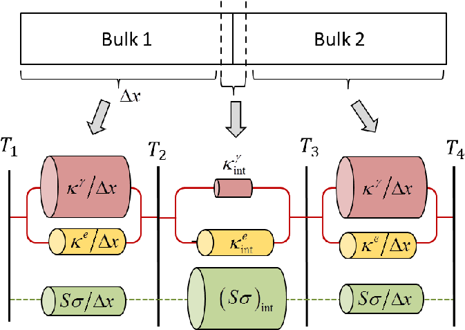
Fig. (3) shows the transport properties of the layer for fixed bulk properties, and varying the interface electrical conductance and phonon thermal conductance (the interface thermopower is fixed). The results are intuitively clear: when the interface electrical conductance is small, it determines the overall layer conductance; conversely when the interface electrical conductance is large, the interface is transparent and the overall conductance is set by the bulk. A similar scenario holds for the thermal conductance (though now the total thermal conductance depends on both electrical and phonon components). I’ve assumed the thermopower is high for all constituents, so that its value is relatively unaffected by the interface. This leads to a $ZT$ value which is enhanced relative to the bulk for a certain range of interfacial transport parameters.

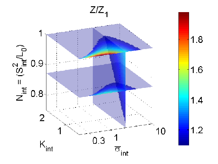
The region of $ZT$ enhancement is shown again in Fig. (4), where only values for which $ZT$ is more than 5% greater than the bulk value are shown. For disordered materials in 2 and 3 dimensions, the phase space of $ZT$ enhancement is very similar to this 3-resistor case, so it’s worth investigating this simple example fully.

In the limit of low interface conductance (the lower left-hand portion of Fig. (4)), the interface properties dominate. $ZT$ of the layer is then approximately that of the interface, so the contours of Fig. (4) in this region are simply those of Eq. (3), with $N\rightarrow N_{\rm int},~K\rightarrow K_{\rm int}$. The small $\sigma_{\rm int}$ in this region implies a small electron thermal conductance $\kappa^{e}_{\rm int}$, via the Wiedamann-Franz law. A large $ZT$ then requires a very small phonon thermal conductance $\kappa_{\rm int}^{\gamma}$, making $ZT$ enhancement in this region difficult to achieve. (Recall that for high thermopower, $ZT$ is set by the ratio of $\kappa^{e}$ to $\kappa^{\gamma}$, see Eq. (3).) In the opposite limit of high interface conductance ($\bar{\sigma}_{\rm int}\gg 1$), the interface is transparent electrically and thermally (thermal transparency follows from Wiedamann-Franz law: $\sigma_{\rm int}\rightarrow\infty\Rightarrow\kappa^{e}_{\rm int}\rightarrow\infty$). Here purely bulk properties are recovered, and $ZT$ is not increased.

The crossover between these limits occurs around $\bar{\sigma}_{\rm int}=1$ (or $\sigma_{\rm int}=\sigma_{1}/\Delta x$), when both interface and bulk properties are important. This is the region most accessible for $ZT$ enhancement. Not surprisingly, $ZT$ is always increased as the phonon thermal conductance of the interface is decreased. I label the maximum value of $K_{\rm int}$ for which there is a $ZT$ enhancement of 5% over the bulk value as $K_{\rm int}^{\rm max}$. (Recall this parameter in full scaled form is $K_{\rm int}^{\max}=\left(\kappa^{\gamma}_{\rm int}/\kappa^{e}_{1}\right)\Delta x$.) This is a key parameter because finding materials with interface scattering that lies below this value is a primary challenge for using nanocomposites for $ZT$ enhancement [16]. I label the associated electrical conductance $\sigma_{\rm int}^{\rm opt}$ (see Fig. (4)). The next section is largely devoted to describing how the values of $K_{\rm int}^{\rm max}$ and $\sigma_{\rm int}^{\rm opt}$ depend on the properties of the bulk material constituents.

So far I have fixed the interface thermopower $S_{\rm int}$. To illustrate how the space of $ZT$ enhancement depends on $S_{\rm int}$, I make some slices through the full parameter space of the interface, shown in Fig. (5). Not surprisingly, as the thermopower of the interface decreases, the space of $ZT$ enhancement in $\left(\bar{\sigma}_{\rm int},~K_{\rm int}\right)$ gets smaller (i.e, it’s harder to achieve enhancement when the interfacial thermopower is weak). In the rest of the paper, I fix $S_{\rm int}=S_{\rm max}$ (or $N_{\rm int}=1$). It should be kept in mind that an interface with smaller $S$ will have more stringent requirements on phonon thermal conductance (i.e a smaller $K_{\rm int}^{\rm max}$) for $ZT$ enhancement.

Moving to disordered materials in 3-d introduces a new system parameter - the concentration of one material with respect to the other. Fig. (6) shows the bulk transport parameters as a function of concentration calculated numerically and with effective medium theory. The interface scattering leads to a decrease in electric and thermal conductivity relative to the bulk values of the constituents. $ZT$ is enhanced relative to the bulk value for a range of concentrations, shown in Fig. (6d). Note there is excellent agreement between effective medium theory and the numeric results; most of the results presented in the rest of the paper are derived from effective medium theory, except where explicitly noted.

The rest of this section describes how the interface properties needed for $ZT$-enhancement depend on the constituent bulk materials. I show that the phase space for $ZT$ enhancement essentially depends only on a small number of parameters of the constituent materials. This is a useful simplification. It enables a precise answer to the question: “given a high-$ZT$ material with thermopower $S_{1}$ and phonon thermal conductivity $\kappa_{1}^{\gamma}$, and another material with $Z$ value $Z_{2}$, what are the interface scattering properties that are required to observe $ZT$ enhancement of the composite material?”. I describe the required interface properties using the parameters $(K_{\rm int}^{\rm max},\sigma_{\rm int}^{\rm opt})$ introduced in the previous section and in Fig. (4).

For each set of bulk and interface properties, I vary the concentration and determine the maximum possible $ZT$ - this maximum value is what is reported in the following results. In all of these results, I assume that the bulk thermopower of the high-$ZT$ constituent is large ($S_{1}=S_{\rm max}$), so that $ZT$ enhancement is a consequence of reducing phonon thermal conductivity.

Fig. (7) is an illustration of how $K_{\rm int}^{\rm max}$ characterizes the phase space of $ZT$ enhancement as bulk materials change. Fig. (7a) shows how the region of enhancement changes as the $ZT$ value of one bulk material component gets smaller. As one component’s $ZT$ value decreases, it’s more difficult to achieve $ZT$ enhancement of the composite via interface scattering. Fig. (7b) shows how this behavior is translated into the parameter $K_{\rm int}^{\rm max}$. In this example, $ZT$ of material 2 is degraded due to a higher phonon thermal conductivity of material 2.

Fig. (8) shows that for a fixed high-$ZT$ constituent, $K_{\rm int}^{\rm max}$ essentially only depends on $Z_{2}$. In Fig. (8a) I show plots of $K_{\rm int}^{\rm max}$ as $Z_{2}T$ is degraded in three different ways: with a “bad” $K_{2}$ (or high phonon thermal conductivity), a “bad” $S_{2}$ (or low thermopower), and a combination of both. Fig. (8b) shows the same thing for a different high-$ZT$ material. Fig. (8b) also shows numeric results (with a “bad $K_{2}$” scenario), which confirm that the effective medium theory and numerical results are very similar. What’s important is that $K_{\rm int}^{\rm max}$ is quite insensitive to how the low-$ZT$ material is deficient. The bulk $ZT$ values of the constituent alone determines the required interfacial phonon scattering for $ZT$ enhancement[13].

Fig. (9a) shows the result of plotting all the curves of Fig. (8) together, normalized by their maximum value. Again a remarkable and useful simplification takes place, where the curves collapse on an approximately “universal” curve. The vertical spread of this normalized curve shows the spread in values for the different curves of Fig. (8).

The right hand-side of the normalized curve of Fig. (9a), where $Z_{2}=Z_{1}$, corresponds to a system with identical bulk phases, with interface scattering between the identical grains. The value of $K_{\rm int}^{\rm max}$ for such a system sets the overall normalization for plots like Fig. (8). In Fig. (8b), I plot the value of this normalization as a function of $K_{\rm bulk}$ and $N_{\rm bulk}$. The two parts of Fig. (9) enable an estimate for the required interface phonon thermal conductance for $ZT$ enhancement.

As an example, let the high-$ZT$ constituent have $N_{1}=0.8$, $K_{1}=2$ (this implies $Z_{1}T=0.36$); this is shown as a white dot in Fig. (9). Fig. (9b) shows the normalization for the $K_{\rm int}^{\rm max}$ curve is 4. Now let the low-$ZT$ material have $Z_{2}T=0.27$, so that $Z_{2}/Z_{1}=0.75$. Using Fig. (9a), I conclude $K_{\rm int}^{\rm max}$ for this material combination is $0.25\times 4=1$ (in dimensionful terms, $K_{\rm int}^{\rm max}=\left(\kappa_{\rm int}^{\gamma}/\kappa_{1}^{e}\right)\Delta x=1$). This means that $ZT$ enhancement requires thermal transport parameters and grain size such that $\left(\kappa_{\rm int}^{\gamma}/\kappa_{1}^{e}\right)\Delta x<1$.

I next go through a similar description of how $\sigma_{\rm int}^{\rm opt}$ depends on bulk material parameters. Fig. (10) shows $\sigma_{\rm int}^{\rm opt}$ as a function of the $Z_{2}/Z_{1}$, for two different high-$ZT$ constituents. I again find that, for fixed high-$ZT$ material, $\sigma_{\rm int}^{\rm opt}$ essentially only depends on $Z_{2}$. Fig. (11a) shows the result of plotting all the curves of Fig. (10) by their maximum value. Again, I find that $\sigma_{\rm int}^{\rm opt}$ as a function of $Z_{2}/Z_{1}$ is an approximately “universal” curve. Fig. (11b) shows the normalization value of this “universal” curve as a function of $N$ and $K$ of the high-$ZT$ constituent. These plots again enable an estimate of $\sigma_{\rm int}^{\rm opt}$ in terms of just a few bulk material parameters.

Returning to the example before (where we assumed a high $ZT$ material with parameters $N_{1}=0.8,~K_{1}=2$, and a low $ZT$ material with $Z_{2}/Z_{1}=0.75$), Fig. (11b) shows the normalization constant of about 5, which is used with Fig. (11a) to infer $\sigma_{\rm int}^{\rm opt}=5\times 0.25=1.25$. In other words, attaining $ZT$ enhancement through interfacial scattering is most easily accessible with a combination of electrical conductivity values and grain size such that $\left(\sigma_{\rm int}/\sigma_{1}\right)\Delta x=1.25$.

$\sigma_{\rm int}^{\rm opt}$ is an important constraint on the interface; even if an interface blocks phonons effectively, if it also blocks electrons too much (i.e has too low $\bar{\sigma}_{\rm int}$), or is transparent to electrons (too high $\bar{\sigma}_{\rm int}$), then it does not lead to overall $ZT$ enhancement. The reason for this is the same as in the simple 3-resistor-in-series case, described earlier. Note that the value of the overall normalization for $\sigma_{\rm int}^{\rm opt}$ is fairly constant over the range of bulk material parameters. Generally, $ZT$ enhancement requires an interface conductance on the order of the bulk conductivity divided by the grain size.

Figs. (9) and (11) represent the main results of the paper. They provide a blueprint to choosing material properties such that a two-component composite results in $ZT$ enhancement. An important aspect of Fig. (9a) is the rapid decrease of $K_{\rm int}^{\rm max}$ as one of the material’s $ZT$ value decreases. This means interfacial phonon scattering can most easily enhance $ZT$ when the two materials have similar $ZT$ values. This poses a key materials science challenge in pursuing this technique for $ZT$ enhancement: often materials with similar (high) $ZT$ values have similar density (i.e. both composed of heavy atoms); however, interfacial phonon scattering is usually strongest between materials with very dissimilar density and speed of sound [16].

For a rough estimate of required material values, the above analysis shows $ZT$ enhancement via interface phonon scattering requires material parameters which satisfy an inequality on the order of $\kappa_{\rm int}^{\gamma}<\kappa_{\rm bulk}^{e}/\Delta x$. A typical thermoelectric has $\kappa_{\rm bulk}^{e}=1~{\rm W/\left(m\cdot K\right)}$. Assuming a grain size of $10~{\rm nm}$, the interface phonon conductance must be less than $10^{8}~{\rm W/\left(m^{2}\cdot K\right)}$ for $ZT$ enhancement. This value is certainly attainable for some material combinations [16], though obtaining this value of $\kappa_{\rm int}^{\gamma}$ for two materials with high $ZT$ values (and low $\kappa_{\rm bulk}^{\gamma}$ values) is likely to be a challenge.

Here I briefly compare the results obtained for the space of $ZT$ enhancement in 1-d, 2-d, and 3-d. The comparison is shown in Fig. (12). The interface parameter space for enhancement is very similar in all cases, but that the enhancement is reduced in higher dimensions. This is because some portion of interface scattering in higher dimensions occurs in directions orthogonal to the transport direction. This scattering is not effective in reducing the phonon thermal conductivity along the overall direction of the temperature gradient, and therefore does not aid in increasing $ZT$. Also shown in Fig. (12) is the concentration in 2-d and 3-d for which the maximum $ZT$ occurs. This value depends on the specific material parameters chosen. For example. if the two bulk materials are equivalent, the optimum enhancement is always at $c=0.5$. As the two bulk materials properties deviate, the optimum concentration moves away from $0.5$ - it’s more advantageous to have a higher concentration of the high-$ZT$ material. At the edge of the phase space of enhancement, the optimum concentration is such that the composite is mostly high-$ZT$ bulk.

To write Eqs. (1) in dimensionless form, I introduce the following variables.

where $L$ is the length of the sample in the transport direction, $T_{0}$ is a fixed reference temperature. This leads to the dimensionless equations:

where $N_{1}=\left(\frac{S_{1}^{2}\sigma_{1}T_{0}}{\kappa_{1}^{e}}\right)$. The prefactor $1/N_{1}$ of the dimensionless conductivity results in an “effective” conductivity $\frac{1}{N_{1}}\left(\frac{\sigma_{i}}{\sigma_{1}}\right)$ that is used when solving Eqs. (V.1). Extracting an effective conductivity from evaluating the charge current response to an electric potential requires accounting for $N_{1}$: $\sigma=N_{1}\left(\frac{j}{\Delta V}\right)$, where $\Delta V$ is the applied potential difference.

The inclusion of interface scattering complicates the scheme used to discretize Eqs. (1-2), which we discuss more fully here. The relevant question is: given a continuous distribution of material, what discrete set of points should we choose to represent the potential and temperature fields? The answer depends on the spatial variation of the fields; to accurately represent the continuous fields requires a more dense mesh near areas of rapid variation in potential and temperature. For example, small interface electrical conductance (compared to the bulk conductivity divided by grain length) implies a sharp potential drop across an interface. This suggests a discretization scheme as shown in Fig. (13a). The conductance on the link separating two plaquettes is set to $\sigma_{\rm int}$ for plaquettes with different identities, and set to $\infty$ otherwise. I call this discretization scheme the “edge scheme”. In two dimensions the sampling may be chosen as shown in Fig. (14a).

In the body of the paper I use a simpler scheme, depicted in Fig. (13b). Here the fields are evaluated at the center of the plaquette, and the interface conductance is put in series with the adjacent bulk conductance a priori. I call this the “center scheme”. This results in a less dense sampling, and is therefore not as accurate as the edge scheme. However, as mentioned in the body of the paper, this scheme is easily adopted to effective medium theory, which is very powerful and much more convenient than direct numerics. To compare the two schemes, I consider a two-component mixture in two dimensions. Fig. (15) shows the $ZT$ value of the composite as I vary the interface electrical conductance $\bar{\sigma}_{\rm int}$ and phonon thermal conductance $K_{\rm int}$. In this case, I let $S_{1}=S_{2}=S_{\rm max}$, so that $ZT$ enhancement is the result of increased phonon scattering. Both schemes give similar results, although the edge scheme shows slightly greater $ZT$ enhancement. In the region of $ZT$ enhancement, the interfacial conductance is not appreciably larger than the bulk, so that the temperature and voltage drops aren’t strongly localized at the interface. This enables the center scheme to represent the fields reasonably well. Moreover the enhancement is due to blocking phonons, or a small $\kappa_{\rm eff}^{\gamma}$. Adding the large bulk $\kappa^{\gamma}_{\rm bulk}$ with the small $\kappa_{\rm int}^{\gamma}$ in series a priori results in an effective $\kappa^{\gamma}$ that’s still small. (For conductors in series, the smallest conductance dominates). I therefore conclude that the approach adopted in the paper works well to describe $ZT$ enhancement via phonon scattering at the interface.

Fig. (16) shows $ZT$ as a function of interface properties for the two schemes when the bulk thermopower is small ($S_{1}=S_{2}=0.5S_{\rm max}$). The role of the interface in $ZT$ enhancement is to provide energy filtering of the electrons, increasing $S$ of the composite. The two schemes’ results are now rather different - the center scheme underestimates the $ZT$ enhancement by a notable margin. This is because energy filtering is accomplished with a sharp temperature drop across the interface, which is not represented in the center scheme. Moreover, adding the low bulk value of $\left(S\sigma\right)_{\rm bulk}$ in series with the high interface $\left(S\sigma\right)_{\rm int}$ a priori leads to a small effective $\left(S\sigma\right)$ (again, when adding these “conductances” in series, the smallest one dominates); the potential increase in $S\sigma$ is partially nullified by the model construction.

References

- [1] J. R. Sootsman, D. Y. Chung, and M. G. Kanatzidis, Angew. Chem. Int. Ed., 48, 8616 (2009).
- [2] M. G. Kanatzidis, Chem. Mater. 22, 648 (2010).
- [3] J. P. Heremans, V. Jovovic, E. S. Toberer, A. Saramat, K. Kurosaki, A. Charoenphakdee, S. Yamanaka, and G. J. Snyder, Science 321, 554 (2008). sig
- [4] J. Martin, L. Wang, L. Chen, and G. S. Nolas, Phys. Rev. B 79, 115311 (2009).
- [5] P. F. P. Poudeu, J. DAngelo, H. Kong, A. Downey, J. L. Short, R. Pcionek, T. P. Hogan, C. Uher, and M. G. Kanatzidis, J. Am. Chem. Soc. 128, 14347 (2006).
- [6] S. V. Faleev and F. Léonard, Phys. Rev. B 77, 214304 (2008).
- [7] A. Popescu, L. M. Woods, J. Martin, and G. S. Nolas, Phys. Rev. B 79, 205302 (2009).
- [8] G. Chen, Phys. Rev. B 57, 14958 (1998).
- [9] The equation of continuity for heat current is generally . In linear response the right-hand-side of this equation can generally be ignored. The full nonlinear version with heating was solved in the numerical calculation, and was found to agree with the results when heating is neglected.
- [10] F. Gather, C. Heiliger and P. J. Klar, J. Phys. Condens. Matter 23, 335301 (2011).
- [11] I. Webman, J. Jortner, and M. H. Cohen, Phys. Rev. B 16, 2959 (1977).
- [12] S. Kirkpatrick, Rev. Mod. Phys. 45, 574 (1973).
- [13] One reason for the insensitivity of to how is decreased is the fact that the absolute differences in parameters along different paths of degradation are relatively small. For example, for , the “bad ” case has , while the “bad ” has . Generally is slightly greater for the “bad ” case. This makes sense, as here the deficiency of material 2 (high conduction of phonons) is more directly addressed by the interface scattering.
- [14] U. Sivan and Y. Imry, Phys. Rev. B 33, 551 (1986).
- [15] R. Venkatasubramanian, E. Siivola, T. Colpitts, and B. OQuinn, Nature 413, 597 (2001).
- [16] D. G. Cahilla, Wayne K. Ford, K. E. Goodson, G. D. Mahan, A. Majumdar, H. J. Maris, R. Merlin, and S. R. Phillpot. App. Phys. Rev. 93, 793 (2003).
- [17] J. Martin, G. S. Nolas, W. Zhang, and L. Chen, App. Phys. Lett. 90, 222112 (2007).
- [18] B. Poudel, Q. Hao, Y. Ma, Y. C. Lan, A. Minnich, B. Yu, X. Yan, D. Wang, A. Muto, D. Vashaee, X. Y. Chen, X. Y, J. M. Liu, M. S. Dresselhaus, G. Chen, Z. Ren, Z. Science 320, 634 (2008).
V Appendix
V.1 Dimensionless variables