On the Power of Manifold Samples in Exploring Configuration Spaces
and the Dimensionality of Narrow Passages

Oren Salzman Michael Hemmer Dan Halperin ^†^†thanks: This work has been supported in part by the 7th Framework Programme for Research of the European Commission, under FET-Open grant number 255827 (CGL—Computational Geometry Learning), by the Israel Science Foundation (grant no. 1102/11), and by the Hermann Minkowski–Minerva Center for Geometry at Tel Aviv University.^†^†thanks: Oren Salzman is with the School for Computer Science, Tel-Aviv University, Tel Aviv 69978, ISRAEL. orenzalz@post.tau.ac.il ^†^†thanks: Michael Hemmer is with the Institute of Operating Systems and Computer Networks, University of Technology Braunschweig, 38106 Braunschweig, GERMANY. mhsaar@googlemail.com ^†^†thanks: Dan Halperin is with the School for Computer Science, Tel-Aviv University, Tel Aviv 69978, ISRAEL. danha@post.tau.ac.il

Abstract

We extend our study of Motion Planning via Manifold Samples (MMS), a general algorithmic framework that combines geometric methods for the exact and complete analysis of low-dimensional configuration spaces with sampling-based approaches that are appropriate for higher dimensions. The framework explores the configuration space by taking samples that are low-dimensional manifolds of the configuration space capturing its connectivity much better than isolated point samples. The scheme is particularly suitable for applications in manufacturing, such as assembly planning, where typically motion planning needs to be carried out in very tight quarters. The contributions of this paper are as follows: (i) We present a recursive application of MMS in a six-dimensional configuration space, enabling the coordination of two polygonal robots translating and rotating amidst polygonal obstacles. In the adduced experiments for the more demanding test cases MMS clearly outperforms PRM, with over 40-fold speedup in a six-dimensional coordination-tight setting. (ii) A probabilistic completeness proof for the case of MMS with samples that are affine subspaces. (iii) A closer examination of the test cases reveals that MMS has, in comparison to standard sampling-based algorithms, a significant advantage in scenarios containing high-dimensional narrow passages. This provokes a novel characterization of narrow passages, which attempts to capture their dimensionality, an attribute that had been (to a large extent) unattended in previous definitions.

Index Terms:

Robot Motion Planning, Narrow Passage, Manifolds, PRM, CGAL

Note to practitioners—Highly constrained motion-planning scenarios, even of low degree of freedom, arise in various applications such as assembly planning and manufacturing applications. Our approach, which emphasizes high precision over any known sampling-based technique that we are aware of, allows to cope with exactly such cases. For instance, we show that our framework can be applied to tight scenarios that arise in three-handed assembly planning. The ability to cope with tight scenarios is possible, in part, due to recent improvements in exact geometric software such as the publicly available Computational Geometry Algorithms Library [41] (CGAL).

I Introduction

Configuration spaces, or C-spaces, are fundamental tools for studying a large variety of systems. A point in a $d$ -dimensional C-space describes one state (or configuration) of a system governed by $d$ parameters. C-spaces appear in diverse domains such as graphical animation, surgical planning, computational biology and computer games. For a general overview of the subject and its applications see, e.g., [11, 29, 31]. The most typical and prevalent example are C-spaces describing mobile systems (“robots”) with $d$ degrees of freedom (dofs) moving in some workspace amongst obstacles. As every point in the configuration space $\mathcal{C}$ corresponds to a free or forbidden pose of the robot, $\mathcal{C}$ decomposes into disjoint sets $\mathcal{C}_{\rm free}$ and $\mathcal{C}_{\rm forb}$ , respectively. Thus, the motion-planning problem is commonly reduced to the problem of finding a path that is fully contained within $\mathcal{C}_{\rm free}$ .

I-A Background

C-spaces for motion planning haven been intensively studied for over three decades. Fundamentally, two major approaches exist:

(i) Analytic solutions: The theoretical foundations, such as the introduction of C-spaces [33] and the understanding that constructing a C-space is computationally hard with respect to the number of dofs [34], were already laid in the late 1970’s and early 1980’s in the context of motion planing. Exact analytic solutions to the general motion-planning problem as well as for various low-dimensional instances have been proposed in [5, 9, 10, 37] and [2, 3, 19, 33, 36], respectively. For a survey of related approaches see [38]. However, only recent advances in applied aspects of computational geometry made robust implementations for important building blocks available. For instance, Minkowski sums, which allow the representation of the C-space of a translating robot, have robust and exact two- and three-dimensional implementations [16, 17, 43]. Likewise, implementations of planar arrangements¹¹ 1 A subdivision of the plane into zero-dimensional, one-dimensional and two-dimensional cells, called vertices, edges and faces, respectively induced by the curves. for curves [41, C.30] [15], could be used as essential components in [37].

(ii) Sampling-based approaches: Sampling-based approaches, such as Probabilistic Roadmaps (PRM) [25], Expansive Space Trees (EST) [21] and Rapidly-exploring Random Trees (RRT) [30], as well as their many variants, aim to capture the connectivity of $\mathcal{C}_{\rm free}$ in a graph data structure, via random sampling of configurations. For a general survey on the approach see [11, 31]. As opposed to analytic solutions these approaches are also applicable to problems with a large number of dof. Importantly, the PRM and RRT algorithms were shown to be probabilistically complete [23, 27, 28], that is, they are guaranteed to find a valid solution, if one exists. However, the required running time for finding such a solution cannot be computed for new queries at run-time. This is especially problematic as these algorithms suffer from high sensitivity to the so-called “narrow passage” problem, e.g., where the robot is required to move in environments cluttered with obstacles, having low clearance.

Though there are also some hybrid approaches [14, 20, 32, 45] that incorporate both analytic and sampling-based approaches, it is apparent that the arsenal of currently available motion-planning algorithms lacks a general scheme applicable to high-dimensional problems with little or low sensitivity to narrow passages. In [35] we introduced a framework for Motion Planning via Manifold Samples (MMS), which also constitutes a hybrid approach. In a three-dimensional C-space it was capable of achieving twenty-fold (and more) speedup factor in running time compared to the PRM algorithm when used for planning paths within narrow passages. We believe that the speedup presented in [35] does not present a mere algorithmic advantage for a specific implemented instance but a fundamental advantage of the framework when solving scenarios with narrow passages. The MMS framework is not the first to consider lower dimensional manifolds of the C-space. Several algorithms attempt to sample in the C-space, and project the sample to lower dimensional manifolds (see, e.g., [8, 40]); however these algorithms still sample points. For cases where some dimensions are presumed to be decoupled, such as multi-robot navigation, one can sample each robot’s individual C-space (see, e.g., [4, 42]) though these algorithms are typically not applicable when there is a tight coupling between the robots.

This study continues developing the MMS framework as a tool to overcome the gap mentioned in existing motion-planning algorithms. We briefly present the scheme and continue to a preliminary discussion on applying MMS in high-dimensional C-spaces, which motivates this paper.

I-B Motion Planning via Manifold Samples

The framework is presented as a means to explore the entire C-space, or, in motion-planning terminology as a multi-query planner, consisting of a preprocessing stage and a query stage. The preprocessing stage constructs the connectivity graph $\mathcal{G}$ of $\mathcal{C}$ , a data structure that captures the connectivity of $\mathcal{C}$ using low-dimensional manifolds as samples. The manifolds are decomposed into cells in $\mathcal{C}_{\rm free}$ and $\mathcal{C}_{\rm forb}$ in an analytic manner; we call a cell of the decomposed manifold that lies in $\mathcal{C}_{\rm free}$ a free space cell (FSC). The FSCs serve as nodes in $\mathcal{G}$ . Two nodes are connected by an edge if their corresponding FSCs intersect. See Fig. 1 for an illustration.

Refer to caption — Fig. 1: MMS in three-dimensional C-spaces of translation and rotation in the plane. The left side illustrates two families of manifolds where the decomposed free cells are darkly shaded. The right side illustrates their intersection, which induces the graph $\mathcal{G}$ . Figure taken from [35].

Once $\mathcal{G}$ has been constructed it can be queried for paths between two configurations $q_{s},q_{t}\in\mathcal{C}_{\rm free}$ in the following manner: A manifold that contains $q_{s}$ in one of its FSCs is generated and decomposed (similarly for $q_{t}$ ). These FSCs and their appropriate edges are added to $\mathcal{G}$ . We compute a path $\gamma$ (of FSCs) in $\mathcal{G}$ between the FSCs that contain $q_{s}$ and $q_{t}$ . If such a path is found in $\mathcal{G}$ , it can be (rather straightforwardly) transformed into a continuous path in $\mathcal{C}_{\rm free}$ by planning a path within each FSC in $\gamma$ .

I-C MMS in Higher Dimensions

The successful application of MMS in [35] to a three-dimensional C-space can be misleading when we come to apply it to higher dimensions. The heart of the scheme is the choice of manifolds from which we sample. Informally, for the scheme to work we must require that the used set of manifolds $\mathcal{M}$ fulfills the following conditions.

C1

The manifolds in $\mathcal{M}$ cover the C-space.
C2

A pair of surfaces chosen uniformly and independently²² 2 The requirement that the choices are independent stems from the way we prove completeness of the method. It is not necessarily an essential component of the method itself. at random from $\mathcal{M}$ intersect with significant probability.
C3

Manifolds need to be of very low dimension as MMS requires an analytic description of the C-space when restricted to a manifold. Otherwise the machinery for the construction of this description is not readily available.

For MMS to work in C-spaces of dimension $d$ , Condition C2 has a prerequisite that the sum of dimensions of a pair of manifolds chosen uniformly and independently at random from $\mathcal{M}$ is at least $d$ with significant probability. This means in particular that $\mathcal{M}$ will consist of manifolds of dimension³³ 3 The precise statement is somewhat more involved and does not contribute much to the informal discussion here. Roughly, $\mathcal{M}$ should comprise manifolds of dimension $\lceil\frac{d}{2}\rceil$ or higher and possibly manifolds of their co-dimension. $\lceil\frac{d}{2}\rceil$ . With this prerequisite in mind, there is already much to gain from using our existing and strong machinery for analyzing two-dimensional manifolds [6, 7, 15], while fulfilling the conditions above: We can solve motion-planning problems with four degrees of freedom, at the strength level that MMS offers, which is higher than that of standard sampling-based tools.

However, we wish to advance to higher-dimensional C-spaces in which satisfying all the above conditions at once is in general impossible. We next discuss two possible relaxations of the conditions above that can lead to effective extensions of MMS to higher dimensions.

Dependent choice of manifolds: If we insist on using only very low-dimensional manifolds even in higher-dimensional C-spaces, then in order to guarantee that pairs of manifolds intersect, we need to impose some dependence between the choices of manifolds, i.e., relaxing condition C2. A natural way to impose intersections between manifolds is to adapt the framework of tree-based planners like RRT [30]. When we add a new manifold, we insist that it connects either directly or by a sequence of manifolds to the set of manifolds collected in the data structure (tree in the case of RRT) so far.

Approximating manifolds of high dimension: As we do not have the machinery to exactly analyze C-spaces restricted to manifolds of dimension three or higher, we suggest to substitute exact decomposition of the manifolds as induced by the C-space by some approximation. i.e., relaxing condition C3. There are various ways to carefully approximate C-spaces. In the rest of the paper we take the approach of a recursive application of MMS.

In Section II we demonstrate this recursive application for a specific problem in a six-dimensional configuration space, namely the coordination of two planar polygonal robots translating and rotating amidst polygonal obstacles. In the adduced experiments for the more demanding test cases MMS clearly outperforms several variants and implementations of PRM with over 40-fold speedup in an especially tight setting. Section III provides the theoretical foundations for using MMS in a recursive fashion. In Section IV we examine the significant advantage of MMS with respect to prevailing sampling-based approaches in scenarios containing high-dimensional narrow passages. This provokes a novel characterization of narrow passages, which attempts to capture their dimensionality. We conclude with an outlook on further work in Section V.

II The Case of Two Rigid Polygonal Robots

We discuss the MMS framework applied to the case of coordinating the motion of two polygonal robots $R_{a}$ and $R_{b}$ translating and rotating in the plane amidst polygonal obstacles. Each robot is described by the position of its reference point $r_{a},r_{b}\in\mathbb{R}^{2}$ and the amount of counter-clockwise rotation $\theta_{a},\theta_{b}$ with respect to an initial orientation. All placements of $R_{a}$ in the workspace $\mathcal{W}$ induce the three-dimensional space $\mathcal{C}^{a}=\mathbb{R}^{2}\times S^{1}$ . Similarly for $R_{b}$ . We describe the full system by the six-dimensional C-space $\mathcal{C}=\mathcal{C}^{a}\times\mathcal{C}^{b}$ .

II-A Recursive Application of the MMS Framework

Had we had the means to decompose three-dimensional manifolds the application of MMS would be straightforward: The set $\mathcal{M}$ consists of two families. An element of the first family of manifolds is defined by fixing $R_{b}$ at free configurations $b\in\mathcal{C}_{\rm free}^{b}$ while $R_{a}$ moves freely inducing the three-dimensional subspaces⁴⁴ 4 In this paper, when discussing subspaces, unless otherwise stated we refer to affine subspaces or linear manifolds. $\mathcal{C}^{a}\times b$ . The second family is defined symmetrically by fixing $a\in R_{a}$ . As subspace pairs of the form $(a\times\mathcal{C}^{b},\mathcal{C}^{a}\times b)$ intersect at the point $(a,b)$ , manifolds of the two families intersect allowing for connections in the connectivity graph $\mathcal{G}$ .

However, we do not have the tools to construct three-dimensional manifolds explicitly. Thus the principal idea is to construct approximations of these manifolds by another application of MMS. Since for a certain manifold one robot is fixed, we are left with a three-dimensional C-space in which the fixed robot is regarded as an obstacle. Essentially this is done by using the implementation presented in [35] but with a simpler set of manifolds (see also Fig. 2): (i) Horizontal slices – corresponding to a fixed orientation of the moving robot while it is free to translate (ii) Vertical lines – corresponding to a fixed location of the reference point of the moving robot while it is free to rotate.

Since we only approximate the three-dimensional subspaces we have to make sure that they still intersect. In other words, if $\mathcal{C}_{\text{apx}}^{a}$ , $\mathcal{C}_{\text{apx}}^{b}$ are the approximations of $\mathcal{C}^{a}$ and $\mathcal{C}^{b}$ , respectively, then $(a\times\mathcal{C}_{\text{apx}}^{b},\mathcal{C}_{\text{apx}}^{a}\times b)$ intersect at the point $(a,b)$ only if $a\in\mathcal{C}_{\text{apx}}^{a}$ and $b\in\mathcal{C}_{\text{apx}}^{b}$ . To ensure this latter condition we sample an initial set of angles $\Theta_{a}$ that is used for the first robot throughout the entire algorithm. When approximating its subspace (the second robot is fixed) we take a horizontal slice for each angle in $\Theta_{a}$ . At the same time, we only fix the robots position at angles in $\Theta_{a}$ . We do the same for the second robot and a set $\Theta_{b}$ . This way it is ensured that even the approximations of the three-dimensional subspaces intersect.

II-B Implementation Details

Horizontal slices: Let $R_{m}$ and $R_{f}$ denote the moving and fixed robot, respectively. $\Theta_{m}$ denotes the set of angles that is sampled for $R_{m}$ . A horizontal plane for an angle $\theta_{m}\in\Theta_{m}$ is defined by the Minkowski sum of $-R_{\theta_{m}}$ with all the obstacles and, in addition, with the fixed robot.⁵⁵ 5 $-R_{\theta_{m}}$ denotes $R_{m}$ rotated around the origin by $\theta_{m}$ and reflected about the origin. However, for each approximation of a three-dimensional affine subspace of the robot $R_{m}$ we are using the same set of angles⁶⁶ 6 We note that in our implementation, we add a random shift to the set of slices to avoid situations where the initial configuration of one of the robots is aligned with a narrow passage (as is the case in Figure 3c). This is done for each robot independently., namely $\Theta_{m}$ . Only the position of the robot $R_{f}$ changes. Therefore, for all $\theta_{m}\in\Theta_{m}$ we precompute the Minkowski sum of $-R_{\theta_{m}}$ with all the obstacles. In order to obtain a concrete slice we only need to add the Minkowski sum of $-R_{\theta_{m}}$ with $R_{f}$ . This can be done by a simple overlay operation (see, e.g., [15, C.6]).

Vertical lines: Fixing the reference point of $R^{m}$ to some location while it is free to rotate induces a vertical line in the three-dimensional C-space. Each vertex (or edge) of the robot in combination with each edge (or vertex) of an obstacle (or the fixed robot) give rise to up to two critical angles on this line. These critical values mark a potential transition between $\mathcal{C}_{\rm forb}$ and $\mathcal{C}_{\rm free}$ . Thus a vertical line is constructed by computing these critical angles and the FSCs are maximal free intervals along this line; (for further details see the Appendix).

II-C Experimental Results

We demonstrate the performance of our planner using three different scenarios in six-dimensional C-spaces. All scenarios consist of a workspace, obstacles, two robots and one query (source and target configurations). Fig. 3 illustrates the scenarios where the obstacles are drawn in blue and the source and target configurations are drawn in green and red, respectively. All reported tests were measured on a Lenovo T420 with a 2.8GHz Intel Core i7-2640M CPU processor and 8GB of memory running with a Windows 7 64-bit OS. Preprocessing times are the average of 12 runs excluding the minimal and maximal values. The algorithm is implemented in C++ based on Cgal [41] and the Boost Graph Library [39], which are used for the geometric primitives, and the connectivity graph $\mathcal{G}$ , respectively.

We chose to compare our planner to the implementation of PRM provided by OMPL [12]. In addition we also compare with Obstacle-Based PRM (OB-PRM) [1] and Uniformly distributed Obstacle-Based PRM (U-OB-PRM) [46] (also implemented in OMPL), which were shown to perform better than PRM in many scenarios where narrow passages exist. We manually optimized the parameters of each planner over a concrete set. The parameters used by MMS are: $n_{\theta}$ – the number of sampled angles; $n_{\ell}$ – the number of vertical lines; $n_{f}$ – the number of times some robot is fixed to a certain configuration while the three-dimensional C-space of the other is computed. The parameters used for the PRM algorithms are: $k$ – the number of neighbors to which each milestone should be connected; res – collision-checking resolution. U-OB-PRM needs additional parameters, the length $l$ of the line-segments sampled in space and the resolution of samples along this line. Following the results of [46] and after validating these parameters, we used the same collision checking-resolution for the resolution and a line-segment of length equal to 10 times the collision-checking resolution. We found empirically that in order to obtain the best results from U-OB-PRM, we should add uniform samples to the biased ones. Thus the variant we used samples half of the time uniformly in space while half of the time uses the scheme suggested in [46]. Table I summarized the parameters used by each algorithm, the average running time and the standard deviation (denoted by $t$ and stdev, respectively).

The Random polygons scenario⁷⁷ 7 A scenario provided as part of the OMPL distribution. is an easy scenario where little coordination is required. Both planners require the same amount of time to solve this case. We see that even though our planner uses complex primitives, when using the right parameters, it can handle simple cases with no overhead when compared to the PRM algorithms.

The Viking-helmet scenario consists of two narrow passages that each robot needs to pass through. Moreover, coordination is required for the two robots to exchange places in the lower chamber. We see that the running times of the MMS implementation are favorable when compared to the PRM implementations. Note that although each robot is required to move along a narrow passage, the motion along this passage does not require coordination between the robots.

The Pacman scenario, in which the two robots need to exchange places, requires coordination of the robots: they are required to move into a position where the C-shaped robot, or Pacman, “swallows” the square robot; the Pacman is then required to rotate around the robot. Finally the two robots should move apart (see Fig. 5). We ran this scenario several times, progressively increasing the square robot size. This caused a “tightening” of the passages containing the desired path. Fig. 4 demonstrates the preprocessing time as a function of the tightness of the problem for both planners. A tightness of zero denotes the base scenario (Fig. 3c) while a tightness of one denotes the tightest solvable case. Our algorithm is less sensitive to the tightness of the problem when compared to the PRM algorithm. In the tightest experiment solved by all PRM variants, MMS runs 10 times faster. We ran the experiment on tighter scenarios but all PRM algorithms crashed after 5000 seconds due to lack of memory resources. We believe that the behavior of the algorithms with respect to the tightness of the passage reveals a fundamental difference between the two algorithms and discuss this in Section IV.

Scenario	MMS					PRM				OB-PRM				U-OB-PRM
	$n_{\theta}$	$n_{\ell}$	$n_{f}$	t[sec]	stdev	k	res	t[sec]	stdev	k	res	t[sec]	stdev	k	res	t[sec]	stdev
Random polygons	5	512	2	8	1.6	10	0.02	14.5	8.3	10	0.01	28.4	12	8	0.01	10.5	9.9
Viking Helmet	20	16	10	6.2	1.2	10	0.005	86.8	34	10	0.005	92.8	14	8	0.0125	40	28
Pacman	5	4	180	17.6	3.5	12	0.015	15	9.5	10	0.01	18.7	6.8	10	0.0125	20	3.3

TABLE I: Comparison of MMS with PRM variants

III Probabilistic Completeness of MMS

An algorithm is probabilistically complete if the probability that it will produce a solution (when one exists) approaches one as more time is spent. It has been shown that PRM, using point samples, is probabilistically complete (see, e.g., [11, C.7]). At first glance it may seem that if the scheme is complete for point samples then it is evidently complete when these samples are substituted with manifold samples: manifolds of dimension one or higher guarantee better coverage of the configuration space. However, there is a crucial difference between PRM and MMS when it comes to connectivity. The completeness proof for PRM relies, among others, on the fact that if the straight line segment in the configuration space connecting two nearby samples lies in the free space, then the nodes corresponding to these two configurations are connected by an edge in the roadmap graph. The connectivity in MMS is attained through intersections of manifolds, which may require a chain of subpaths on several distinct manifolds to connect two nearby free configurations. This is what makes the completeness proof for MMS non trivial and is expressed in Lemma III.3 below.

We present a probabilistic completeness proof for the MMS framework for the case where the C-space $\mathcal{C}$ is the d-dimensional Euclidean space $\mathbb{R}^{d}$ , while MMS is taking samples from two perpendicular affine subspaces, the sum of dimensions of which is $d$ . Assuming that the C-space is Euclidean does not impose a real restriction as long as the actual C-space can be embedded in a Euclidean space (see, e.g. [11, Section 3.5, Section 7.1.2], [31, Chapters 4-5] or [26]).

Let $A$ and $B$ denote affine subspaces of $\mathcal{C}$ and let $k$ and $d-k$ be their dimensions, respectively. As $\mathcal{C}$ is decomposed into two perpendicular subspaces, a point $p=(a_{1},\dots,a_{k},b_{1},\dots,b_{d-k})\in\mathcal{C}$ may be represented as the pair of points $(a,b)$ from subspaces $A$ and $B$ . Under this assumption, the set of manifolds $\mathcal{M}$ consists of two families of $k$ and $(d-k)$ -dimensional manifolds $\mathcal{M}^{A}$ and $\mathcal{M}^{B}$ . Family $\mathcal{M}^{A}$ consists of all manifolds that are defined by fixing a point $a_{0}\in A$ while the remaining $d-k$ parameters are variable; $\mathcal{M}^{B}$ is defined symmetrically. Two manifolds $m(a)\in\mathcal{M}^{A}$ and $m(b)\in\mathcal{M}^{B}$ always intersect in exactly one point, i.e., $m(a)\cap m(b)=(a,b)\in\mathcal{C}$ . Let $B^{\mathcal{C}}_{r}(p)=\{q\in\mathcal{C}~|~dist(p,q)\leq r\}$ define a ball in $\mathcal{C}$ of radius $r$ centered at $p\in\mathcal{C}$ , where $dist$ denotes the Euclidean metric on $\mathcal{C}$ . Likewise, $B^{B}_{r}(b)$ and $B^{A}_{r}(a)$ denote $(d-k)$ and $k$ -dimensional balls in $B$ and $A$ , respectively.

Definition III.1 ( $\rho$ -intersecting).

For $\rho>0$ we call a manifold $m(a)\in\mathcal{M}^{A}$ $\rho$ -intersecting for a point $p\in\mathcal{C}$ if $m(a)\cap B^{\mathcal{C}}_{\rho}(p)\neq\emptyset$ , i.e., if $a\in B^{A}_{\rho}(p_{A})$ , where $p_{A}$ is the projection of $p$ onto $A$ . Similarly for manifolds in $B$ .

A feasible path $\gamma$ is a continuous mapping from the interval $[0,1]$ into $\mathcal{C}_{\rm free}$ . The image of a path is defined as $Im(\gamma)=\{\gamma(\alpha)\ |\ \alpha\in[0,1]\}$ . We show that for any collision-free path $\gamma_{p,q}$ of clearance $\rho>0~$ between two configurations $p$ and $q$ the MMS constructs a path from $p$ to $q$ such that (i) the path lies on the FSCs of the sampled manifolds and (ii) every point on the path is at distance at most $\rho$ from $\gamma_{p,q}$ , with a positive probability. Moreover, the probability of failing to find such a path by the MMS algorithm decreases exponentially with the number of samples.

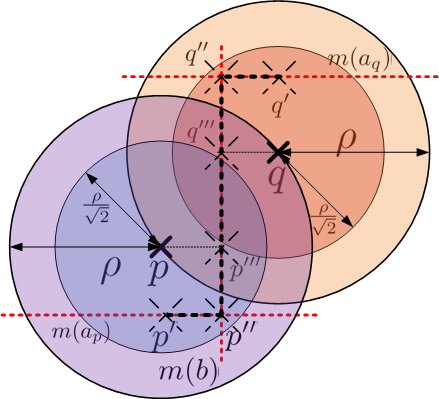
Lemma III.2.

For $p\in\mathcal{C}$ and $\rho>0$ let $m(a)\in\mathcal{M}^{A}$ and $m(b)\in\mathcal{M}^{B}$ be two manifolds that are $\rho/\sqrt{2}$ -intersecting for $p$ . Their intersection point $p^{\prime}=(a,b)=m(a)\cap m(b)$ is in $B^{\mathcal{C}}_{\rho}(p)$ .

Proof.

$m(a)$ is $\rho/\sqrt{2}$ -intersecting for $p$ . Hence, we know that the distance of $a$ to $p_{A}$ is less than $\rho/\sqrt{2}$ , the same holds for $b$ and $p_{B}$ . Thus we can conclude (as demonstrated in Fig. 6a):

dist(p,p^{\prime})=\sqrt{dist(p_{A},a)^{2}+dist(p_{B},b)^{2}}\leq\rho.

∎

The following lemma shows that for any two points $p$ and $q$ , a manifold $m(b)\in\mathcal{M}^{B}$ that is close to both points enables a connection between two manifolds $m(a_{p}),m(a_{q})\in\mathcal{M}^{A}$ that are close to $p$ and $q$ , respectively.

Lemma III.3.

Let $p,q\in C$ be two points such that $dist(p,q)\leq\rho$ and let $m(a_{p}),m(a_{q})\in\mathcal{M}^{A}$ be two $\rho/\sqrt{2}$ -intersecting manifolds for $p$ and $q$ respectively. Let $m(b)\in\mathcal{M}^{B}$ be a manifold that is simultaneously $\rho/\sqrt{2}$ -intersecting for $p$ and $q$ and let $p^{\prime}=(a_{p},p_{B})\in B_{\rho}^{\mathcal{C}}(p)$ and $q^{\prime}=(a_{q},q_{B})\in B_{\rho}^{\mathcal{C}}(q)$ be the projection of $p$ and $q$ on $m(a_{p})$ and $m(a_{q})$ , respectively.

There exists a path $\gamma_{p^{\prime},q^{\prime}}$ between $p^{\prime}$ and $q^{\prime}$ such that $Im(\gamma_{p^{\prime},q^{\prime}})\subseteq(B_{\rho}^{\mathcal{C}}(p)\cup B_{\rho}^{\mathcal{C}}(q))\cap(m(a_{p})\cup m(b)\cup m(a_{q}))$ , i.e., there is a path lying on the manifolds within the union of the balls.

Proof.

Let $p^{\prime\prime}=m(a_{p})\cap m(b)=(a_{p},b)$ and $q^{\prime\prime}=m(a_{q})\cap m(b)=(a_{q},b)$ denote the intersection point of $m(a_{p})$ and $m(a_{q})$ with $m(b)$ , respectively. Moreover, let $p^{\prime\prime\prime}=(p_{A},b)\in B_{\rho}^{\mathcal{C}}(p)$ and $q^{\prime\prime\prime}=(q_{A},b)\in B_{\rho}^{\mathcal{C}}(q)$ denote the projections of $p$ and $q$ on $m(b)$ . We show that the path which is the concatenation of the segments $(p^{\prime},p^{\prime\prime}),~(p^{\prime\prime},p^{\prime\prime\prime}),~(p^{\prime\prime\prime},q^{\prime\prime\prime}),~(q^{\prime\prime\prime},q^{\prime\prime})$ and $(q^{\prime\prime},q^{\prime})$ lies on $(m(a_{p})\cup m(b)\cup m(a_{q}))$ within the union of the balls $(B_{\rho}^{\mathcal{C}}(p)\cup B_{\rho}^{\mathcal{C}}(q))$ . See Fig. 6b.

By Lemma III.2 the intersection points $p^{\prime\prime}$ and $q^{\prime\prime}$ are inside $B_{\rho}^{\mathcal{C}}(p)$ and $B_{\rho}^{\mathcal{C}}(q)$ , respectively. Thus, by convexity of each ball the segments $(p^{\prime},p^{\prime\prime})\subset m(q_{p})$ and $(q^{\prime},q^{\prime\prime})\subset m(a_{q})$ as well as the segments $(p^{\prime\prime},p^{\prime\prime\prime}),(q^{\prime\prime},q^{\prime\prime\prime})\subset m(b)$ are in $(B_{\rho}^{\mathcal{C}}(p)\cup B_{\rho}^{\mathcal{C}}(q))$ .

It remains to show that $(p^{\prime\prime\prime},q^{\prime\prime\prime})\subset m(b)$ is inside $(B_{\rho}^{\mathcal{C}}(p)\cup B_{\rho}^{\mathcal{C}}(q))$ . Recall that $dist(p,q)\leq\rho$ and therefore $dist(p^{\prime\prime\prime},q^{\prime\prime\prime})\leq\rho$ . Let $\bar{p}$ be a point on the segment $(p^{\prime\prime\prime},q^{\prime\prime\prime})$ that, w.l.o.g, is closer to $p^{\prime\prime\prime}$ . Thus $dist(\bar{p},p^{\prime\prime\prime})\leq\rho/2$ . The manifold $m(b)$ is $\rho/\sqrt{2}$ -intersecting, thus $dist(p,p^{\prime\prime\prime})\leq\rho/\sqrt{2}$ . As the segments $(p,p^{\prime\prime\prime})$ and $(p^{\prime\prime\prime},\bar{p})$ are perpendicular it holds:

$\displaystyle dist(p,\bar{p})$	$\displaystyle=$	$\displaystyle\sqrt{dist(p,p^{\prime\prime\prime})^{2}+dist(p^{\prime\prime\prime},\bar{p})^{2}}$
	$\displaystyle\leq$	$\displaystyle\sqrt{\rho^{2}/2+\rho^{2}/4}$
	$\displaystyle<$	$\displaystyle\rho.$

∎

Theorem III.4.

Let $p,q$ be points in $\mathcal{C}_{\rm free}$ such that there exists a collision-free path $\gamma_{p,q}\in\Gamma$ of length $L$ and clearance $\rho$ between $p$ and $q$ . Then the probability of the MMS algorithm to return a path between $p$ and $q$ after generating $n_{A}$ and $n_{B}$ manifolds from families $\mathcal{M}^{A}$ and $\mathcal{M}^{B}$ as above, respectively is:

			$\displaystyle Pr[(p,q){\rm SUCCESS}]$
		$\displaystyle=$	$\displaystyle 1-Pr[(p,q){\rm FAILURE}]$
		$\displaystyle\geq$	$\displaystyle 1-\left\lceil\frac{L}{\rho}\right\rceil\left[\left(1-\mu_{A}\right)^{n_{A}}+\left(1-\eta_{B}\right)^{n_{B}}\right],$

where $\mu_{A}$ and $\eta_{B}$ are some positive constants smaller than 1.

Proof.

Let $l=\left\lceil L/\rho\right\rceil$ , there exists a sequence $[p_{0}\ldots p_{\ell}]$ such that $p_{i}\in Im(\gamma_{p,q})$ , $p_{0}=p$ , $p_{\ell}=q$ , $B_{\rho}(p_{i})\in\mathcal{C}_{\rm free}$ and $dist(p_{i},p_{i+1})\leq\rho$ . MMS adds the manifolds $m(p_{A})$ and $m(q_{A})$ to the connectivity graph.

Let $A^{\prime}\subset A$ , $|A^{\prime}|=n_{A}$ and $B^{\prime}\subset B$ , $|B^{\prime}|=n_{B}$ , be the two point sets that define the manifolds $M^{A^{\prime}}$ and $M^{B^{\prime}}$ that are used by the MMS algorithm. If there is a subset $\{m(a_{1})\ldots m(a_{\ell-1})\}\subseteq M^{A^{\prime}}$ and a subset $\{m(b_{1})\ldots m(b_{\ell-1})\}\subseteq M^{B^{\prime}}$ such that $(p_{i},p_{i+1},m(a_{i}),m(b_{i}),m(a_{i+1}))$ fulfill the conditions of Lemma III.3 for $i\in\{0\ldots\ell-1\}$ , then there exists a path from $p$ to $q$ in the FSCs constructed by the MMS framework, namely the path which is the concatenation of paths constructed in Lemma III.3. This implies that $p$ and $q$ are in the same connected component of $\mathcal{G}$ , which implies that MMS constructs a path in $\mathcal{C}_{\rm free}$ from $p$ to $q$ .

Let $I_{1}\ldots I_{\ell-1}$ be a set of indicator variables such that each $I_{i}$ witnesses the event that there is a $\rho/\sqrt{2}$ -intersecting manifold for $p_{i}$ in $M^{A^{\prime}}$ . (For $p_{0}$ and $p_{\ell}$ this is trivially the case due the explicit construction of $m(p_{A})$ and $m(q_{A})$ .) Let $J_{0}\ldots J_{\ell-1}$ be a set of indicator variables such that each $J_{i}$ witnesses the event that there is a manifold in $M^{B^{\prime}}$ that is simultaneously $\rho/\sqrt{2}$ -intersecting for $p_{i}$ and $p_{i+1}$ . It follows that MMS succeeds in answering the query $(p,q)$ if $I_{i}=1$ for all $1\leq i\leq\ell-1$ and $J_{j}=1$ for all $0\leq j\leq\ell-1$ . Therefore,

	$\displaystyle Pr[(p,q){\rm FAILURE}]$	$\displaystyle\leq$	$\displaystyle Pr\left(\vee^{\ell-1}_{i=1}(I_{i}=0)\vee^{\ell-1}_{j=0}(J_{j}=0)\right)$
		$\displaystyle\leq$	$\displaystyle\sum^{\ell-1}_{i=1}Pr[I_{i}=0]+\sum^{\ell-1}_{j=0}Pr[J_{j}=0].$

The events $I_{i}=0$ and $J_{j}=0$ are independent since the samples are taken independent. Thus the probability $Pr[I_{i}=0]$ , i.e., that not even one of the $n_{A}$ samples from $A$ is $\rho/\sqrt{2}$ -intersecting for $p_{i}$ is $(1-\mu_{A})^{n_{A}}$ , where $\mu_{A}$ is the probability measure that a random sample $a\in A$ defines a manifold that is $\rho/\sqrt{2}$ -intersecting for a certain point $p\in\mathcal{C}$ . Thus, $\mu_{A}$ is obviously positive. Similarly, $Pr[J_{i}=0]=(1-\eta_{B})^{n_{B}}$ , where $\eta_{B}$ is the probability measure that a random sample $b\in B$ defines a manifold that is $\rho/\sqrt{2}$ -intersecting for a two specific points $p,q\in\mathcal{C}$ with $dist(p,q)<\rho$ , that is, it is proportional to the volume of the intersection $B^{B}_{\rho/\sqrt{2}}(p_{B})\cap B^{B}_{\rho/\sqrt{2}}(q_{B})$ , which is positive since the radius of the balls is larger than $\rho/2$ . Since the sampling is uniform and independent:

	$\displaystyle Pr[(p,q){\rm FAILURE}]$	$\displaystyle\leq$	$\displaystyle\left\lceil\frac{L}{\rho}-1\right\rceil\left(1-\mu_{A}\right)^{n_{A}}+\left\lceil\frac{L}{\rho}\right\rceil\left(1-\eta_{B}\right)^{n_{B}}$
		$\displaystyle\leq$	$\displaystyle\left\lceil\frac{L}{\rho}\right\rceil\left[\left(1-\mu_{A}\right)^{n_{A}}+\left(1-\eta_{B}\right)^{n_{B}}\right].$

∎

It follows that as $n_{A}$ and $n_{B}$ tend to $\infty$ , the probability of failing to find a path under the conditions stated in Theorem III.4 tends to zero.

Recursive application The proof of Theorem III.4 assumes that the samples are taken using full high-dimensional manifolds. However, Section II demonstrates a recursive application of MMS where the approximate samples are generated by another application of MMS.

In order to obtain a completeness proof for the two-level scheme let $\gamma$ be a path of clearance $2\rho$ . First, assume that the samples taken by the first level of MMS are exact. Applying Theorem III.4 for $\gamma$ and $\rho$ shows that with sufficient probability MMS would find a set $M^{\prime}$ of manifolds that would contain a path $\gamma^{\prime}$ . Since we required clearance $2\rho$ but relied on the tighter clearance $\rho$ , it is guaranteed that $\gamma^{\prime}$ still has clearance $\rho$ . Now, each manifold $m^{\prime}\in\mathcal{M}^{\prime}$ is actually only an approximation constructed by another application of MMS. Thus, for each $m^{\prime}\in\mathcal{M}^{\prime}$ apply Theorem III.4 to the subpath $\gamma^{\prime}_{m^{\prime}}=\gamma^{\prime}\cap m^{\prime}$ which has clearance $\rho$ . Concatenation of all the resulting subpaths concludes the argument. Of course the parameters in the inequality in Theorem III.4 change accordingly.

We remark that the recursive approach imposes a mild restriction on the sampling scheme as the sampling and the approximation must be somewhat coordinated. Since in theory $m(a)\cap m(b)=(a,b)$ we must ensure that points that we sample from $A$ are contained in every approximation of $m(b)\in\mathcal{M}^{B}$ and vise versa. In our implementation this is ensured by restricting the set of possible angles to those used to approximate $m(b)\in\mathcal{M}^{B}$ (see Section II).

IV On the Dimension of Narrow Passages

Consider the Pacman scenario illustrated in Fig. 3c of the experiments section. We obtain a narrow passage by increasing the size of the square-shaped robot making it harder for the Pacman to swallow it. Fig. 4 shows that our approach is significantly less sensitive to this tightening of the free space than the PRM algorithm. In order to explain this, let us take a closer look at the nature of the narrow passage for the tightest solvable case.

In order to get from the start placement to the goal placement, the Pacman must swallow the square, rotate around it and spit it out again. We concentrate on the swallowing motion. Fig. 7 depicts the tightest case, i.e., when the square robot fits exactly into the “mouth” of the Pacman. The gray rectangle indicates the positions of the reference point of the square such that there is a valid movement of the Pacman, considering the walls of the room, that will allow it to swallow the square robot (two-dimensional region, two parameters). The rotation angle of the square is also important (one additional parameter). The range of concurrently possible values for all three parameters is small but does not tend to zero either. The passage becomes only narrow by the fact that the rotation angle of the Pacman must correlate exactly with the orientation of the square to allow for passing through the mouth. Moreover, the set of valid placements for the reference point of the Pacman while swallowing the square (other parameters being fixed) is a line, i.e., its $x$ and $y$ parameter values are coupled. Thus, the passage is a four-dimensional object as we have a tight coupling of two pairs of parameters in a six-dimensional C-space.

The PRM approach has difficulties to sample in this passage since the measure tends to zero as the size of the square increases. On the other hand, for our approach the passage is only narrow with respect to the correlation of the two angles. As soon as the MMS samples an (approximated) volume that fixes the square robot such that the Pacman can engulf it, the approximation of the volume just needs to include a horizontal slice of a suitable angle and the passage becomes evident in the corresponding Minkowski sum computation.

IV-A Definition of Narrow Passages

Intuition may suggest that narrow passages are tunnel-shaped. However, a one-dimensional tunnel in a high-dimensional C-spaces would correspond to a simultaneous coupling of all parameters, which is often not the case. For instance, the discussion of the Pacman scenario shows that the passage is narrow but that it is still a four-dimensional volume, which proved to be a considerable advantage for our approach in the experiments. Although some sampling based approaches try to take the dimension of a passage into account (see e.g. [13]) it seems that this aspect is not reflected by existing definitions that attempt to capture attributes of the C-space. Definitions such as $\epsilon$ -goodness [24] and expansiveness [21] are able to measure the size of a narrow passage better than the clearance [23] of a path, but neither incorporates the dimension of a narrow passage in a very accessible way. Therefore, we would like to propose a new set of definitions that attempt to simultaneously grasp the narrowness and the dimension of a passage.

We start by defining the “ordinary” clearance of a path in $\mathcal{C}_{\rm free}$ . The characterization is based on the notion of homotopy classes of paths with respect to a set $\Gamma_{s,t}$ , i.e., the set of all paths starting at $s$ and ending at $t$ . For a path $\gamma_{0}\in\Gamma_{s,t}$ and its homotopy class $\mathcal{H}(\gamma_{0})$ we define the clearance of the class as the largest clearance found among all paths in $\mathcal{H}(\gamma_{0})$ .

Definition IV.1.

The clearance of a homotopy class $\mathcal{H}(\gamma_{0})$ for $\gamma_{0}\in\Gamma_{s,t}$ is

\sup_{\gamma\in\mathcal{H}(\gamma_{0})}\\ \{~\sup\{~\rho>0~|~B_{\rho}^{d}\oplus Im(\gamma)\subseteq\mathcal{C}_{\rm free}~\}~\},

where $\oplus$ denotes the Minkowski sum of two sets, which is the vector sum of the sets.

By using a $d$ -dimensional ball this definition treats all directions equally, thus considering the passage of $\mathcal{H}(\gamma_{0})$ to be a one-dimensional tunnel. We next refine this definition by using a $k$ -dimensional disk, which may be placed in different orientations depending on the position along the path.

Definition IV.2.

For some integer $0<\boldsymbol{k}\leq d$ the $\boldsymbol{k}$ -clearance of $\mathcal{H}(\gamma_{0})$ is:

\sup_{\gamma\in\mathcal{H}(\gamma_{0})}\{\rho>0|\forall t\in[0,1]\exists{\tt R}\in{\cal R}:\gamma(t)\oplus{\tt R}(t)B^{k}_{\rho}\subseteq\mathcal{C}_{\rm free}\},

where ${\cal R}$ is the set of $d$ -dimensional rotation matrices and $B^{k}_{\rho}$ is the $k$ -dimensional ball of radius $\rho$ . In case ${\tt R}$ is required to change continuously we talk about continuous $\boldsymbol{k}$ -clearance.

Clearly, the $k$ -clearance of $\mathcal{H}(\gamma_{0})$ for $k=d$ is simply the clearance of $\mathcal{H}(\gamma_{0})$ . For decreasing values of $k$ , the $k$ -clearance of a homotopy class is a monotonically increasing sequence. We next define the dimension of a passage using this sequence, that is, we set the dimension to be the first $k$ for which the clearance becomes significantly larger⁸⁸ 8 We leave this notion informal as it might depend on the problem at hand. than the original $d$ -dimensional clearance.

Definition IV.3.

A passage for $\mathcal{H}(\gamma_{0})$ in $\mathbb{R}^{d}$ of clearance $\rho$ (see Def. IV.1) is called $\boldsymbol{d-k+1}$ -dimensional if $k$ is the largest index such that $k$ -clearance $(\mathcal{H}(\gamma_{0}))\gg\rho$ . If for every $k$ $k$ -clearance $(\mathcal{H}(\gamma_{0}))\not\gg\rho$ then we call the passage one-dimensional⁹⁹ 9 For simplicity of definition we chose to stop at the largest index $k$ for which $k$ -clearance $\gg\rho$ . One could contemplate alternative more elaborate definitions that keep on searching for even larger clearance for smaller indices.

For instance, both passages in Figure 8 have a measure of $\varepsilon^{2}$ thus for a PRM like planner, sampling in either passage is equally hard as the probability of a uniform point sample to lie in either one of the narrow passages is proportional to $\varepsilon^{2}$ . However, the two passages are fundamentally different. The passage depicted on the right-hand side is a one-dimensional tunnel corresponding to a tight coupling of the three parameters. The passage depicted on the left-hand side is a two-dimensional flume which is much easier to intersect by a probabilistic approach that uses manifolds as samples. Our new definitions formally reveal this difference. For $k$ equals 3, 2 and 1 the $k$ -clearance of the right passage is $\varepsilon$ , $\sqrt{2}\varepsilon$ and larger than $1$ , respectively. For the left passage this sequence is $\varepsilon^{2}$ for $k=3$ and larger than $1$ for $k=2,1$ which characterizes the passage as two-dimensional.

IV-B Discussion

We believe that the definitions introduced in Section IV-A, can be an essential component of a formal proof that shows the advantage of manifold samples over point samples in the presence of high-dimensional narrow passages. We sketch the argument briefly. Let $\mathcal{C}_{\rm free}$ contain a narrow passage of dimension $k$ , that is, the passage has clearance $\rho$ and $k$ -clearance $\lambda$ , where $\lambda\gg\rho$ . This implies that it is possible to place discs of dimension $k$ and radius $\lambda\gg\rho$ into the tight passage. The main argument is that for a random linear manifold of dimension $d-k$ the probability to hit such a disc is proportional to $\lambda$ , which is much larger than $\rho$ . The probability also depends on the angle between the linear subspace containing the disc and the linear manifold. However, by choosing a proper set of manifold families it is possible to guarantee the existence of at least one family for which this angle is bounded, independent of the orientation of the disk.

V Further Work

The extension of MMS [35] presented here is part of our on-going efforts towards the goal of creating a general scheme for exploring high-dimensional C-spaces that is less sensitive to narrow passages than currently available tools. As discussed in Section I-C the original scheme imposes a set of conditions that in combination restrict an application of MMS to rather low dimensions. In this paper we chose to relax condition C3, for example by computing only approximations of three-dimensional manifolds. An alternative path is to relax condition C2, for example by not sampling the manifolds uniformly and independently at random. This would enable the use of manifolds of low dimension as it allows to enforce intersection. Following this path we envision a single-query planner that explores a C-space in an RRT-like fashion. Using these extensions we wish to apply the scheme to a variety of difficult problems including assembly maintainability (part removal for maintenance [47]) by employing a single-query variant of the scheme.

Another possibility is to explore other ways to compute approximative manifold samples, for instance, the (so far) exact representations of FSCs could be replaced by much simpler (and thus faster) but conservative¹⁰¹⁰ 10 Approximated FSCs are contained in $\mathcal{C}_{\rm free}$ . approximations. This is certainly applicable to manifold samples of dimension one or two and should also enable manifold samples of higher dimensions. We remark that the use of approximations should not harm the probabilistic completeness as long as it is possible to refine the approximations such that they converge to the exact results.

In order to demonstrate the potential of the scheme, we adapted our motion planner to the problem of three-handed translational assembly planning. In assembly planning [44, 18], we are given a collection of parts, and the goal is to assemble the parts into one (given) object. Typically, the problem is tackled by starting at the end configuration and recursively separating the object into sub-groups. Informally, the number of groups that may be considered simultaneously is the number of hands used. The problem, which is known in general to be computationally hard (see, e.g., [22], has been studied extensively for two hands but little has been done for more.

The first assembly-planning problem we consider, depicted in Fig. 9a demonstrates a scenario where the two purple parts need to move in alternations in order to exit a surrounding part (the obstacle) in order to reach a disassembled configuration. This problem was solve by our planner within 37 seconds (average over 10 runs) and could not be solved by the PRM algorithm (which was terminated after 10 minutes). The RRT algorithm managed solving this scenario within 160 seconds with a success rate of 50% (if the solution was not found within 10 minutes the run was consiedered unsuccesfull; average over 10 runs). The second assembly-planning problem, depicted in Fig. 9b demonstrates a scenario where multiple purple parts need to be moved out of the surrounding green part. At each iteration, two purple parts are chosen at random and the planner attempts to translate both parts (as independent parts) out of the obstacle. The most interesting case occurs when the lower triangles have been removed and the two M-shaped parts need to translate out of the obstacle. In order for this to occur, the left M-shaped part needs to translate to the bottom-left corner for the right M-shaped part to be able to translate out of the obstacle. Our planner manages to plan this in under one second (average over 10 runs) while this case could not be solved by either the RRT or PRM algorithms (which were terminated after 10 minutes). We note that this is not the traditional assembly-planning formulation as the parts are not touching each other. In order for a sampling-based algorithm (such as MMS) to be applicable, some slack is required between the parts. However, the slack can be much smaller when using MMS as opposed to standard sampling-based planners.

(a)

(b)

Fig. 9: Three-handed assembly-planning scenarios. Static obstacle (first hand) is depicted in green and moving parts (second and third hands) are colored. In (b), at each iteration two moving parts are chosen randomly while the remaining parts are considered part of the static obstacles (if they were not disassembled in previous iterations).

Finally, we intend to extend the scheme to and experiment with motion-planning problems for highly-redundant robots as well as for fleets of robots, exploiting the symmetries in the respective C-space.

For supplementary material, omitted here for lack of space, the reader is referred to our project web-page http://acg.cs.tau.ac.il/projects/mms.

References

[1] N. M. Amato and Y. Wu. A randomized roadmap method for path and manipulation planning. In ICRA, pages 113–120, 1996.
[2] B. Aronov and M. Sharir. On translational motion planning of a convex polyhedron in 3-space. SIAM J. Comput., 26(6):1785–1803, 1997.
[3] F. Avnaim, J.-D. Boissonnat, and B. Faverjon. A practical exact motion planning algorithm for polygonal object amidst polygonal obstacles. In Proceedings of the Workshop on Geometry and Robotics, pages 67–86, London, UK, 1989. Springer-Verlag.
[4] N. Ayanian and V. Kumar. Decentralized feedback controllers for multiagent teams in environments with obstacles. IEEE Transactions on Robotics, 26(5):878–887, 2010.
[5] S. Basu, R. Pollack, and M.-F. Roy. Algorithms in Real Algebraic Geometry. Algorithms and Computation in Mathematics. 2nd Edition, Springer-Verlag, 2006.
[6] E. Berberich, E. Fogel, D. Halperin, M. Kerber, and O. Setter. Arrangements on parametric surfaces II: Concretizations and applications. MCS, 4:67–91, 2010.
[7] E. Berberich, E. Fogel, D. Halperin, K. Mehlhorn, and R. Wein. Arrangements on parametric surfaces I: General framework and infrastructure. Mathematics in Computer Science, 4:45–66, 2010.
[8] D. Berenson, S. S. Srinivasa, and J. J. Kuffner. Task space regions: A framework for pose-constrained manipulation planning. I. J. Robotic Res., 30(12):1435–1460, 2011.
[9] J. F. Canny. Complexity of Robot Motion Planning (ACM Doctoral Dissertation Award). The MIT Press, June 1988.
[10] B. Chazelle, H. Edelsbrunner, L. J. Guibas, and M. Sharir. A singly exponential stratification scheme for real semi-algebraic varieties and its applications. Theoretical Computer Science, 84(1):77 – 105, 1991.
[11] H. Choset, W. Burgard, S. Hutchinson, G. Kantor, L. E. Kavraki, K. Lynch, and S. Thrun. Principles of Robot Motion: Theory, Algorithms, and Implementation. MIT Press, June 2005.
[12] I. A. Şucan, M. Moll, and L. E. Kavraki. The Open Motion Planning Library. IEEE Robotics & Automation Magazine, 19(4):72–82, 2012.
[13] S. Dalibard and J.-P. Laumond. Linear dimensionality reduction in random motion planning. I. J. Robotic Res., 30(12):1461–1476, 2011.
[14] M. De Berg, O. Cheong, M. van Kreveld, and M. Overmars. Computational Geometry: Algorithms and Applications. 3nd Edition, Springer, 2008.
[15] E. Foegl, D. Halperin, and R. Wein. CGAL Arrangements and their Applications. Springer, Heidelberg, 2012.
[16] E. Fogel and D. Halperin. Exact and efficient construction of Minkowski sums of convex polyhedra with applications. Computer Aided Design, 39(11):929–940, 2007.
[17] P. Hachenberger. Exact Minkowksi sums of polyhedra and exact and efficient decomposition of polyhedra into convex pieces. Algorithmica, 55(2):329–345, 2009.
[18] D. Halperin, J.-C. Latombe, and R. H. Wilson. A general framework for assembly planning: The motion space approach. Algorithmica, 26(3-4):577–601, 2000.
[19] D. Halperin and M. Sharir. A near-quadratic algorithm for planning the motion of a polygon in a polygonal environment. Disc. Comput. Geom., 16(2):121–134, 1996.
[20] S. Hirsch and D. Halperin. Hybrid motion planning: Coordinating two discs moving among polygonal obstacles in the plane. In WAFR 2002, pages 225–241.
[21] D. Hsu, J. Latombe, and R. Motwani. Path planning in expansive configuration spaces. Int. J. Comp. Geo. & App., 4:495–512, 1999.
[22] L. E. Kavraki and M. N. Kolountzakis. Partitioning a planar assembly into two connected parts is np-complete. Inf. Process. Lett., 55(3):159–165, 1995.
[23] L. E. Kavraki, M. N. Kolountzakis, and J.-C. Latombe. Analysis of probabilistic roadmaps for path planning. IEEE Trans. Robot. Automat., 14(1):166–171, 1998.
[24] L. E. Kavraki, J.-C. Latombe, R. Motwani, and P. Raghavan. Randomized query processing in robot path planning. J. Comput. Syst. Sci, 57(1):50–60, August 1998.
[25] L. E. Kavraki, P. Svestka, J.-C. Latombe, and M. Overmars. Probabilistic roadmaps for path planning in high dimensional configuration spaces. IEEE Trans. Robot. Automat., 12(4):566–580, 1996.
[26] J. J. Kuffner. Effective sampling and distance metrics for 3d rigid body path planning. In ICRA, pages 3993–3998, 2004.
[27] J. J. Kuffner and S. M. Lavalle. RRT-Connect: An efficient approach to single-query path planning. In ICRA, pages 995–1001, 2000.
[28] A. M. Ladd and L. E. Kavraki. Generalizing the analysis of PRM. In ICRA, pages 2120–2125, May 2002.
[29] J.-C. Latombe. Robot Motion Planning. Kluwer Academic Publishers, Norwell, MA, USA, 1991.
[30] S. M. Lavalle. Rapidly-exploring random trees: A new tool for path planning. In Computer Science Dept., Iowa State University, Tech. Rep:98–11, 1998.
[31] S. M. LaValle. Planning Algorithms. Cambridge University Press, Cambridge, U.K., 2006.
[32] J.-M. Lien. Hybrid motion planning using Minkowski sums. In RSS 2008.
[33] T. Lozano-Perez. Spatial planning: A configuration space approach. MIT AI Memo 605, 1980.
[34] J. H. Reif. Complexity of the mover’s problem and generalizations. In FOCS, pages 421–427, Washington, DC, USA, 1979. IEEE Computer Society.
[35] O. Salzman, M. Hemmer, B. Raveh, and D. Halperin. Motion planning via manifold samples. Algorithmica, 67(4):547–565, 2013.
[36] J. T. Schwartz and M. Sharir. On the ”piano movers” problem: I. The case of a two-dimensional rigid polygonal body moving amidst polygonal barriers. Commun. Pure appl. Math, 35:345 – 398, 1983.
[37] J. T. Schwartz and M. Sharir. On the ”piano movers” problem: II. General techniques for computing topological properties of real algebraic manifolds. Advances in Applied Mathematics, 4(3):298 – 351, 1983.
[38] M. Sharir. Algorithmic Motion Planning, Handbook of Discrete and Computational Geometry. 2nd Edition, CRC Press, Inc., Boca Raton, FL, USA, 2004.
[39] J. G. Siek, L.-Q. Lee, and A. Lumsdaine. The Boost Graph Library: User Guide and Reference Manual. Addison-Wesley Professional, 2001.
[40] M. Stilman. Task constrained motion planning in robot joint space. In IROS, pages 3074–3081, 2007.
[41] The CGAL Project. CGAL User and Reference Manual. CGAL Editorial Board, 3.7 edition, 2010. http //www.cgal.org/.
[42] G. Wagner, M. Kang, and H. Choset. Probabilistic path planning for multiple robots with subdimensional expansion. In ICRA, pages 2886–2892, 2012.
[43] R. Wein. Exact and efficient construction of planar Minkowski sums using the convolution method. In ESA, pages 829–840, 2006.
[44] R. H. Wilson and J.-C. Latombe. Geometric reasoning about mechanical assembly. Artificial Intelligence, 71:371–396, 1994.
[45] J. Yang and E. Sacks. RRT path planner with 3 DOF local planner. In ICRA, pages 145–149, 2006.
[46] H.-Y. Yeh, S. L. Thomas, D. Eppstein, and N. M. Amato. UOBPRM: A uniformly distributed obstacle-based PRM. In IROS, pages 2655–2662, 2012.
[47] L. Zhang, X. Huang, Y. J. Kim, and D. Manocha. D-plan: Efficient collision-free path computation for part removal and disassembly. In Journal of Computer-Aided Design and Applications, 2008.

Critical Values for Rotating Robot

We consider a polygonal robot rotating about a fixed reference point amidst polygonal obstacles. As the position of the robot is fixed the considered manifold is a vertical line in the configuration space, whose endpoints are identified. Thus, we parameterize the manifold with $\tau\in\mathbb{P(R)}$ . On this manifold we are interested in the FSCs, which are bounded by critical values. A critical value indicates a potential transition between $\mathcal{C}_{\rm free}$ and $\mathcal{C}_{\rm forb}$ , i.e., a configuration where the robot is in contact with an obstacles. More precisely: Either a robot’s edge is in contact with an obstacle’s vertex or a robot’s vertex is in contact with an obstacle’s edge. These cases will be referred to as vertex-edge contacts and edge-vertex contacts, respectively. The rest of this section introduces the necessary notions to analyze the problem.

A robot $R$ is a simple polygon with vertices $\{v_{1},\dots,v_{n}\}$ , where $v_{i}=(x_{i},y_{i})^{T}$ and edges $\{(v_{1},v_{2}),\dots(v_{n},v_{1})\}$ . We assume that the reference point of $R$ is located at the origin. The position of $R$ in the workspace is defined by a configuration $q=(r_{q},\theta_{q})$ , where $r_{q}=(x_{q},y_{q})^{T}$ . Thus, $q$ maps the position of a vertex $v_{i}$ as follows:

v_{i}(q)=\left[\begin{array}[]{cc}\cos\theta&-\sin\theta\\ \sin\theta&\cos\theta\end{array}\right]v_{i}+r_{q}.

Given a fixed point $p=(x_{p},y_{p})^{T}$ we define in Equation 1 the parameterization $(p,\tau)\in\mathbb{R}^{2}\times\mathbb{R}\mathbb{P}^{1}$ which fixes the robot’s reference point to a specific location.

x_{q}=x_{p},\ \ \ y_{q}=y_{p},\ \ \ \theta_{q}=2\arctan\tau.

(1)

A parameterized vertex is represented in Equation (2)

v_{i}(p,\tau)=\frac{1}{1+\tau^{2}}\left[\begin{array}[]{cc}1-\tau^{2}&-2\tau\\ 2\tau&1-\tau^{2}\end{array}\right]v_{i}+p.

(2)

Robot’s vertex - Obstacle’s edge

Let $r_{q}=(x_{q},y_{q})^{T}$ be the robot’s fixed location. Let $v_{i}$ be a robot’s vertex and let $v_{o_{1}}$ and $v_{o_{1}}$ be the obstacle’s edge’s endpoints. The obstacle’s edge can be parameterized as $e_{o}(s)=v_{o1}+s(v_{o2}-v_{o1})$ , where $s\in[0,1]$ . If the distance between the fixed reference point and the obstacle’s edge is larger than the distance between the robot’s vertex and its reference point, then the edge cannot impose a constraint. Namely all the edges $e$ such that $d(r_{q},e)\geq d(r_{q},v_{i})$ may be filtered out. A criticality occurs when the robot’s vertex coincides with the edge $e$ , thus $e(s)=v_{i}(r_{q},\tau)$ . This yields the following equalities:

x_{o1}+s(x_{o2}-x_{o1})=\frac{1-\tau^{2}}{1+\tau^{2}}x_{i}-\frac{2\tau y_{i}}{1+\tau^{2}}+x_{q}

y_{o1}+s(y_{o2}-y_{o1})=\frac{2\tau}{1+\tau^{2}}x_{i}+\frac{1-\tau^{2}}{1+\tau^{2}}y_{i}+y_{q}

Multiplication with $(1+\tau^{2})$ yields

(1+\tau^{2})(x_{o1}+s(x_{o2}-x_{o1}))=(1-\tau^{2})x_{i}-(2\tau)y_{i}+x_{q}(1+\tau^{2})

(1+\tau^{2})(y_{o1}+s(y_{o2}-y_{o1}))=(2\tau)x_{i}+(1-\tau^{2})y_{i}+y_{q}(1+\tau^{2})

Or,

			$\displaystyle s(1+\tau^{2})(x_{o2}-x_{o1})(y_{o2}-y_{o1})$
		$\displaystyle=$	$\displaystyle[(1-\tau^{2})x_{i}-(2\tau)y_{i}+(1+\tau^{2})(x_{q}-x_{o1})](y_{o2}-y_{o1})$
			$\displaystyle s(1+\tau^{2})(x_{o2}-x_{o1})(y_{o2}-y_{o1})$
		$\displaystyle=$	$\displaystyle[(2\tau)x_{i}+(1-\tau^{2})y_{i}+(1+\tau^{2})(y_{q}-y_{o1})](x_{o2}-x_{o1})$

denoting $\Delta_{ox}=x_{o2}-x_{o1}$ , and $\Delta_{oy}=y_{o2}-y_{o1}$ :

			$\displaystyle[(1-\tau^{2})x_{i}-(2\tau)y_{i}+(1+\tau^{2})(x_{q}-x_{o1})]\Delta_{oy}$
		$\displaystyle=$	$\displaystyle[(2\tau)x_{i}+(1-\tau^{2})y_{i}+(1+\tau^{2})(y_{q}-y_{o1})]\Delta_{ox}$

Finally:

k_{2}\tau^{2}+k_{1}\tau+k_{0}=0,

(3)

where

$\displaystyle k_{2}$	$\displaystyle=$	$\displaystyle(x_{q}-x_{o1}-x_{i})\Delta_{oy}-(y_{q}-y_{o1}-y_{i})\Delta_{ox}$
$\displaystyle k_{1}$	$\displaystyle=$	$\displaystyle-2(y_{i}\Delta_{oy}+x_{i}\Delta_{ox})$
$\displaystyle k_{0}$	$\displaystyle=$	$\displaystyle(x_{q}-x_{o1}+x_{i})\Delta_{oy}-(y_{q}-y_{o1}+y_{i})\Delta_{ox}$
$\displaystyle\Delta_{ox}$	$\displaystyle=$	$\displaystyle x_{o2}-x_{o1},$
$\displaystyle\Delta_{oy}$	$\displaystyle=$	$\displaystyle y_{o2}-y_{o1}.$

The solutions to Equation 3 are two parameterized angles $\tau_{j}$ , where $j\in\{1,2\}$ . The corresponding position on the line can be identified by substituting $\tau$ with $\tau_{j}$ in one of the two equations for $s$ , where at least one is well defined as at least $(x_{o2}-x_{o1})$ or $(y_{o2}-y_{o1})$ does not vanish.

s=\frac{(1-\tau^{2})x_{i}-(2\tau)y_{i}+(1+\tau^{2})(x_{q}-x_{o1})}{(x_{o2}-x_{o1})(1+\tau^{2})}

s=\frac{(2\tau)x_{i}+(1-\tau^{2})y_{i}+(1+\tau^{2})(y_{q}-y_{o1})}{(y_{o2}-y_{o1})(1+\tau^{2})}

If $s_{j}\in[0,1]$ , then the corresponding point is indeed on the edge and the value represents a potential transitions between $\mathcal{C}_{\rm free}$ and $\mathcal{C}_{\rm forb}$ .

Robot’s edge - Obstacle’s vertex

Let $r_{q}=(x_{q},y_{q})^{T}$ be the fixed robot’s location. Let $v_{1},v_{2}$ be the robot’s vertex such that the robot’s edge is defined as $e(s,r_{q},\tau)=v_{1}(r_{q},\tau)+s(v_{2}(r_{q},\tau)-v_{1}(r_{q},\tau))$ for $s\in[0,1]$ and $v_{o}$ be the obstacle’s vertex. If the distance between the fixed reference point and the obstacle’s vertex is larger than the distance between the robot’s two vertices and its reference point, then the vertex cannot impose a constraint. Namely, all the obstacle vertices $v_{o}$ such that $d(r_{q},v_{0})\geq d(r_{q},v_{i})$ may be filtered out. A criticality occurs when a point on the robot’s edge coincides with the obstacle’s vertex, namely for some $s\in[0,1]$ :

	$\displaystyle v_{ox}$	$\displaystyle=$	$\displaystyle v_{1x}(p,\tau)+s(v_{2x}(p,\tau)-v_{1x}(p,\tau))$
	$\displaystyle v_{oy}$	$\displaystyle=$	$\displaystyle v_{1y}(p,\tau)+s(v_{2y}(p,\tau)-v_{1y}(p,\tau))$

Eliminating $s$ we obtain

			$\displaystyle(v_{ox}-v_{1x}(p,\tau))(v_{2y}(p,\tau)-v_{1y}(p,\tau))$
		$\displaystyle=$	$\displaystyle(v_{oy}-v_{1y}(p,\tau))(v_{2x}(p,\tau)-v_{1x}(p,\tau)).$

Denoting $\Delta_{x}=v_{2x}-v_{1x}$ and $\Delta_{y}=v_{2y}-v_{1y}$ :

			$\displaystyle(v_{ox}-v_{1x}(p,\tau))(2\tau\Delta_{x}+(1-\tau^{2})\Delta_{y})$
		$\displaystyle=$	$\displaystyle(v_{oy}-v_{1y}(p,\tau))((1-\tau^{2})\Delta_{x}-2\tau\Delta_{y}).$

Denoting $a=(v_{ox}-x_{q})$ and $b=(v_{oy}-y_{q})$
and $k=v_{1x}v_{2y}-v_{2x}v_{1y}$ , we obtain

l_{2}\tau^{2}+l_{1}\tau+l_{0}=0,

(4)

where

$\displaystyle l_{2}$	$\displaystyle=$	$\displaystyle a\Delta_{y}-b\Delta_{x}+k,$
$\displaystyle l_{1}$	$\displaystyle=$	$\displaystyle-2(a\Delta_{x}+b\Delta_{y}),$
$\displaystyle l_{0}$	$\displaystyle=$	$\displaystyle-l_{2}+2k,$
$\displaystyle\Delta_{x}$	$\displaystyle=$	$\displaystyle v_{2x}-v_{1x},$
$\displaystyle\Delta_{y}$	$\displaystyle=$	$\displaystyle v_{2y}-v_{1y}.$

Similarly to the case of a robot’s vertex in contact with an obstacles edges the solutions to Equation 4 are two parameterized angles $\tau_{j}$ , for $j\in\{1,2\}$ , that represent potential transitions between $\mathcal{C}_{\rm free}$ and $\mathcal{C}_{\rm forb}$ . Again, these angles may represent intersections that are not on the robot’s edge but on the line supporting the edge. Namely, if we obtain $s_{j}$ by plugging $\tau_{j}$ into either one of the two following equations and $s_{j}\notin[0,1]$ then we should not consider the corresponding $\tau_{j}$ .

	$\displaystyle s$	$\displaystyle=$	$\displaystyle\frac{v_{ox}-v_{1x}(p,\tau)}{v_{2x}(p,\tau)-v_{1x}(p,\tau)}$
	$\displaystyle s$	$\displaystyle=$	$\displaystyle\frac{v_{oy}-v_{1y}(p,\tau)}{v_{2y}(p,\tau)-v_{1y}(p,\tau)}$

On the Power of Manifold Samples in Exploring Configuration Spaces and the Dimensionality of Narrow Passages

Abstract

Index Terms:

I Introduction

I-A Background

I-B Motion Planning via Manifold Samples

I-C MMS in Higher Dimensions

II The Case of Two Rigid Polygonal Robots

II-A Recursive Application of the MMS Framework

II-B Implementation Details

II-C Experimental Results

III Probabilistic Completeness of MMS

Definition III.1 (ρ\rho-intersecting).

Lemma III.2.

Proof.

Lemma III.3.

Proof.

Theorem III.4.

Proof.

IV On the Dimension of Narrow Passages

IV-A Definition of Narrow Passages

Definition IV.1.

Definition IV.2.

Definition IV.3.

IV-B Discussion

V Further Work

References

Critical Values for Rotating Robot

Robot’s vertex - Obstacle’s edge

Robot’s edge - Obstacle’s vertex

On the Power of Manifold Samples in Exploring Configuration Spaces
and the Dimensionality of Narrow Passages

Definition III.1 ( $\rho$ -intersecting).