Triadic Measures on Graphs: The Power of Wedge SamplingThanks: This work was funded by the DARPA Graph-theoretic Research in Algorithms and the Phenomenology of Social Networks (GRAPHS) program and by the DOE ASCR Complex Interconnected Distributed Systems (CIDS) program, and Sandia’s Laboratory Directed Research & Development (LDRD) program. Sandia National Laboratories is a multi-program laboratory managed and operated by Sandia Corporation, a wholly owned subsidiary of Lockheed Martin Corporation, for the U.S. Department of Energy’s National Nuclear Security Administration under contract DE-AC04-94AL85000.
Abstract
Graphs are used to model interactions in a variety of contexts, and there is a growing need to quickly assess the structure of a graph. Some of the most useful graph metrics, especially those measuring social cohesion, are based on triangles. Despite the importance of these triadic measures, associated algorithms can be extremely expensive. We propose a new method based on wedge sampling. This versatile technique allows for the fast and accurate approximation of all current variants of clustering coefficients and enables rapid uniform sampling of the triangles of a graph. Our methods come with provable and practical time-approximation tradeoffs for all computations. We provide extensive results that show our methods are orders of magnitude faster than the state-of-the-art, while providing nearly the accuracy of full enumeration. Our results will enable more wide-scale adoption of triadic measures for analysis of extremely large graphs, as demonstrated on several real-world examples.
1 Introduction
Graphs are used to model infrastructure networks, the World Wide Web, computer traffic, molecular interactions, ecological systems, epidemics, citations, and social interactions, among others. Despite the differences in the motivating applications, some topological structures have emerged to be important across all these domains. triangles, which can be explained by homophily (people become friends with those similar to themselves) and transitivity (friends of friends become friends). This abundance of triangles, along with the information they reveal, motivates metrics such as the clustering coefficient and the transitivity ratios [29, 30]. The triangle structure of a graph is commonly used in the social sciences for positing various theses on behavior [11, 21, 7, 14]. Triangles have also been used in graph mining applications such as spam detection and finding common topics on the WWW [13, 4]. The authors’ earlier work used distribution of degree-wise clustering coefficients as the driving force for a new generative model, Blocked Two-Level Erdös-Rényi [23]. The authors’ have also observed that relationships among degrees of triangle vertices can be a descriptor of the underlying graph [12].
1.1 Clustering coefficients
The information about triangles is usually summarized in terms of clustering coefficients. Let be a simple undirected graph with vertices and edges. Let denote the number of triangles in the graph and be the number of wedges (a path of length ). The most common measure is the global clustering coefficient , which measures how often friends of friends are also friends. We show that we can achieve speed-ups of up to four orders of magnitude with extremely small errors; see Fig. 1 and Fig. 2.


Our approach is not limited to clustering coefficients, however. A per-vertex clustering coefficient, , is defined as the fraction of wedges centered at that participate in triangles. The mean value of is called the local clustering coefficient, . A more nuanced view of triangles is given by the degree-wise clustering coefficients. This is a set of values indexed by degree, where is the average clustering coefficient of degree vertices. In addition to degree distribution, many graphs are characterized by plotting the clustering coefficients, i.e., versus . We summarize our notation and give formal definitions in Tab. 1.
| number of vertices | |
| number of vertices of degree | |
| number of edges | |
| degree of vertex | |
| set of degree- vertices | |
| total number of wedges | |
| number of wedges centered at vertex | |
| total number of triangles | |
| number of triangles incident to vertex | |
| number of triangles incident to a degree vertex |
| global clustering coefficient | |
| clustering coefficient of vertex | |
| local clustering coefficient | |
| degree-wise clustering coefficient |
1.2 Related Work
There has been significant work on enumeration of all triangles [8, 22, 18, 5, 9]. Recent work by Cohen [10] and Suri and Vassilvitskii [24] give parallel implementations of these algorithms. Arifuzzaman et al. [1] give a massively parallel algorithm for computing clustering coefficients. Enumeration algorithms however, can be very expensive, since graphs even of moderate size (millions of vertices) can have an extremely large number of triangles (see e.g., Tab. 2). Eigenvalue/trace based methods have been used by Tsourakakis [25] and Avron [2] to compute estimates of the total and per-degree number of triangles. However, computing eigenvalues (even just a few of them) is a compute-intensive task and quickly becomes intractable on large graphs.
Most relevant to our work are sampling mechanisms. Tsourakakis et al. [26] started the use of sparsification methods, the most important of which is Doulion [28]. This method sparsifies the graph by keeping each edge with probability ; counts the triangles in the sparsified graph; and multiplies this count by to predict the number of triangles in the original graph. Various theoretical analyses of this algorithm (and its variants) have been proposed [17, 27, 20]. One of the main benefits of Doulion is that it reduces large graphs to smaller ones that can be loaded into memory. However, their estimate can suffer from high variance [31]. Alternative sampling mechanisms have been proposed for streaming and semi-streaming algorithms [3, 16, 4, 6].
Yet, all these fast sampling methods only estimate the number of triangles and give no information about other triadic measures.
1.3 Our contributions
In this paper, we introduce the simple yet powerful technique of wedge sampling for counting triangles. Wedge sampling is really an algorithmic template, as opposed to a single algorithm, as various algorithms can be obtained from the same basic structure. Some of the salient features of this method are:
- •
Versatility of wedge sampling: We show how to use wedge sampling to approximate the various clustering coefficients: , , and . From these, we can estimate the numbers of triangles: and . Moreover, our techniques can even be extended to find uniform random triangles, which is useful for computing triadic statistics. Other sampling methods are usually geared towards only and .
- •
Provably good results with precise bounds: The mathematical analysis of this method is a direct consequence of standard Chernoff-Hoeffding bounds. We obtain explicit time-error-accuracy tradeoffs. In other words, if we want an estimate for with error at most 10% with probability at least 99.9% (say), we know we need only 380 wedge samples. This estimate is independent of the size of the graph, though the preprocessing required by our method is linear in the number of edges (to obtain the degree distribution).
- •
Fast and scalable: Our estimates converge rapidly, well within the theoretical bounds provided. Although there is no other method that competes directly with wedge sampling, we compare with Doulion [28]. Our experimental studies show that our wedge sampling algorithm is far faster, when the variances of the two methods are similar (see Tab. 5 in the appendix). We do not compare to eigenvalue-based approaches since they are much more expensive for larger graphs.
2 The wedge sampling method
We present the general method of wedge sampling for estimating clustering coefficients. In later sections, we instantiate this for different algorithms.
We say a wedge is closed if it is part of a triangle; otherwise, we say the wedge is open. Thus, in Fig. 3, -- is an open wedge, while -- is a closed wedge. The middle vertex of a wedge is called its center, i.e., wedges -- and -- are centered at .

Wedge sampling is best understood in terms of the following thought experiment. Fix some distribution over wedges and let be a random wedge. Let be the indicator random variable that is if is closed and otherwise. Denote .
Suppose we wish to estimate . We simply generate independent random wedges , with associated random variables . Define as our estimate. The Chernoff-Hoeffding bounds give guarantees on , as follows.
Theorem 2.1 (Hoeffding [15])
Let be independent random variables with for all . Define . Let . Then for , we have
Hence, if we set , then . In other words, with confidence at least , the error in our estimate is at most .
Fig. 4 shows the number of samples needed for different error rates. We show three different curves for difference confidence levels. Increasing the confidence has minimal impact on the number of samples. The number of samples is fairly low for error rates of 0.1 or 0.01, but it increases with the inverse square of the desired error.

3 Computing the global clustering coefficient and the number of triangles
| Time | |||||||
|---|---|---|---|---|---|---|---|
| Graph | (secs) | ||||||
| amazon0312 | 401K | 2350K | 69M | 3686K | 0.160 | 0.421 | 0.261 |
| amazon0505 | 410K | 2439K | 73M | 3951K | 0.162 | 0.427 | 0.269 |
| amazon0601 | 403K | 2443K | 72M | 3987K | 0.166 | 0.430 | 0.268 |
| as-skitter | 1696K | 11095K | 16022M | 28770K | 0.005 | 0.296 | 90.897 |
| cit-Patents | 3775K | 16519K | 336M | 7515K | 0.067 | 0.092 | 3.764 |
| roadNet-CA | 1965K | 2767K | 6M | 121K | 0.060 | 0.055 | 0.095 |
| web-BerkStan | 685K | 6649K | 27983M | 64691K | 0.007 | 0.634 | 54.777 |
| web-Google | 876K | 4322K | 727M | 13392K | 0.055 | 0.624 | 0.894 |
| web-Stanford | 282K | 1993K | 3944M | 11329K | 0.009 | 0.629 | 6.987 |
| wiki-Talk | 2394K | 4660K | 12594M | 9204K | 0.002 | 0.201 | 20.572 |
| youtube | 1158K | 2990K | 1474M | 3057K | 0.006 | 0.128 | 2.740 |
| flickr | 1861K | 15555K | 14670M | 548659K | 0.112 | 0.375 | 567.160 |
| livejournal | 5284K | 48710K | 7519M | 310877K | 0.124 | 0.345 | 102.142 |
We use the wedge sampling scheme to estimate the global clustering coefficient, . Consider the uniform distribution on wedges. We can interpret as the probability that a uniform random wedge is closed or, alternately, the fraction of closed wedges.
To generate a uniform random wedge, note that the number of wedges centered at vertex is and . We set to get a distribution over the vertices. Note that the probability of picking is proportional to the number of wedges centered at . A uniform random wedge centered at can be generated by choosing two random neighbors of (without replacement).
Claim 3.1
Suppose we choose vertex with probability and take a uniform random pair of neighbors of . This generates a uniform random wedge.
Consider some wedge centered at vertex . The probability that is selected is . The random pair has probability of . Hence, the net probability of is .
Alg. 1 shows the randomized algorithm -wedge sampler for estimating in a graph . Combining the bound of Thm. 2.1 with Claim 3.1, we get the following theorem.
Theorem 3.1
Set . The algorithm -wedge sampler outputs an estimate for the clustering coefficient such that with probability greater than .
Note that the number of samples required is independent of the graph size, but computing does depend on the number of edges, .
To get an estimate on , the number of triangles, we output , which is guaranteed to be within of with probability greater than .
3.1 Experimental results
We implemented our algorithms in C and ran our experiments on a computer equipped with a 2.3GHz Intel core i7 processor with 4 cores and 256KB L2 cache (per core), 8MB L3 cache, and an 8GB memory. We performed our experiments on 13 graphs from SNAP [32] and per private communication with the authors of [19]. In all cases, directionality is ignored, and repeated and self-edges are omitted. The properties of these matrices are presented in Tab. 2, where , , , and are the numbers of vertices, edges, wedges, and triangles, respectively. And and correspond to the global and local clustering coefficients. The last column reports the times for the enumeration algorithm. Our enumeration algorithm is based on the principles of [8, 22, 10, 24], such that each edge is assigned to its vertex with a smaller degree (using the vertex numbering as a tie-breaker), and then vertices only check wedges formed by edges assigned to them for closure.
As seen in Fig. 1 wedge sampling works orders of magnitude faster than the enumeration algorithm. Detailed results on times can be seen in Tab. 3 in the appendix. The timing results show tremendous savings; for instance, wedge sampling only takes 0.015 seconds on as-skitter while full enumeration takes 90 seconds.
Fig. 2 show the accuracy of the wedge sampling algorithm. Again detailed results on times can be seen in Tab. 3 in the appendix. At 99.9% confidence (), the upper bound on the error we expect for 2K, 8K, and 32K samples is .043, .022, and .011, respectively. Most of the errors are much less than the bounds would suggest. For instance, the maximum error for 2K samples is .007, much less than that 0.43 given by the upper bound. Fig. 5 shows the fast convergence of the clustering coefficient estimate (for the graph amazon0505) as the number of samples increases. The dashed line shows the error bars at 99.9% confidence. In all our experiments, the real error is always much smaller than what is indicated by Thm. 2.1.

4 Computing the local clustering coefficient
We now demonstrate how a small change to the underlying distribution on wedges allows us to compute the local clustering coefficient, . Alg. 2 shows the procedure -wedge sampler. The only difference between -wedge sampler and -wedge sampler is in picking random vertex centers. Vertices are picked uniformly instead of from the distribution .
Theorem 4.1
Set . The algorithm -wedge sampler outputs an estimate for the clustering coefficient such that with probability greater than .
Let us consider a single sampled wedge , and let be the indicator random variable for the wedge being closed. Let be the uniform distribution on wedges. For any vertex , let be the uniform distribution on pairs of neighbors of . Observe that
We will show that this is exactly .
For a single sample, the probability that the wedge is closed is exactly . The bound of Thm. 2.1 completes the proof.
Fig. 6 and Fig. 7 present the results of our experiments for computing the local clustering coefficients. More detailed results can be found Tab. 4 in the appendix. Experimental setup and the notation are the same as in §3.1. The results again show that wedge sampling provides accurate estimations with tremendous improvements in runtime. In this case, we come closer to the theoretical error bounds. For instance, the largest different in the 2K sample case is 0.017, which is much closer to the theoretical error bound of 0.043.


5 Computing degree-wise clustering
coefficients and triangle estimates
We demonstrate the power of wedge sampling by estimating the degree-wise clustering coefficients . We also provide a sampling algorithm to estimate , the number of triangles incident to degree- vertices. Alg. 3 shows procedure -wedge sampler.
Theorem 5.1
Set . The algorithm -wedge sampler outputs an estimate for the clustering coefficient such that with probability greater than .
The proof of the following is similar to that of Thm. 4.1. Since is the average clustering coefficient of a degree vertex, we can apply the same arguments as in Thm. 4.1.
By modifying the template given in §2, we can also get estimates for . Now, instead of simply counting the fraction of closed wedges, we take a weighted sum. Alg. 4 describes the procedure -wedge sampler. We let denote the total number of wedges centered at degree vertices.
Theorem 5.2
Set . The algorithm -wedge sampleroutputs an estimate for the with the following guarantee: with probability greater than .
For a single sampled wedge , we define . We will argue that the expected value of is exactly below. Once we have that, an application of the Hoeffding bound of Thm. 2.1 shows that with probability greater than . Multiplying this inequality by , we get , completing the proof.
To show , partition the set of wedges centered on degree vertices into four sets . The set () contains all closed wedges containing exactly degree- vertices. The remaining open wedges go into . For a sampled wedge , if , then . If , then nothing is added. The wedge is a uniform random wedge from those centered on degree- vertices. Hence, .
Now partition the set of triangles involving degree vertices into three sets , where is the set of triangles with degree vertices. Observe that . If a triangle has vertices of degree , then there are exactly wedges centered in degree vertices (in that triangle). So, . Therefore, .
5.1 Computing the clustering coefficient for bins of vertices
Algorithms in the previous section present how to compute the clustering coefficient of vertices of a given degree. In practice, it may be sufficient to compute clustering coefficients over bins of degrees. Wedge sampling algorithms can still be extended for bins of degrees by a small adjustment of the sampling procedure. Within each bin, we weight each vertex according to the number of wedges it produces. This guarantees that each wedge in the bin is equally likely to be selected.
5.2 Experimental results
Fig. 8 shows results on three graphs for clustering coefficients; the remaining figures are shown in the Fig. 12 in the appendix. The data is grouped in logarithmic bins of degrees, i.e., . In other words, form the -th bin. We show the estimates with increasing number of samples. At 8K samples, the error is expected to be less than 0.02, which is apparent in the plots. Observe that even 500 samples yields a reasonable estimate in terms of the differences by degree.
Fig. 9 shows the time to calculate all values, showing a tremendous savings in runtime as a result of using wedge sampling. In this figure, runtimes are normalized with respect to the runtimes of full enumeration. As the figure shows, wedge sampling takes only a tiny fraction of the time of full enumeration especially for large graphs.

6 Generating a uniform sample of the triangles
While most triadic measures focus on the number of triangles and their distribution, the triangles themselves, not only their count, can reveal a lot of information about the graph. The authors’ recent work [12] has looked at the relations among the degrees of the vertices of triangles. In these experiments, a full enumeration of the triangles was used, which limited the sizes of the graphs we could use. To avoid this computational burden, a uniform sampling of the triangles can be used.
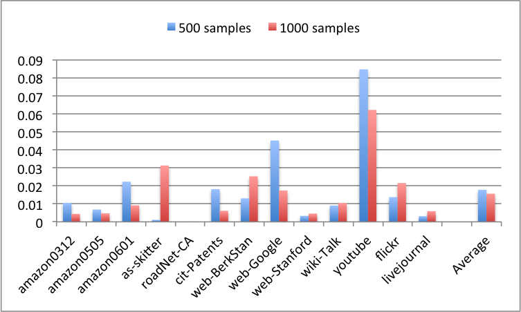
Wedge sampling provides a uniform sampling the triangles of a graph. Consider the uniform wedge sampling of Alg. 1. Some of these wedges will be closed, so we generate a random set of triangles. Each such triangle is an independent, uniform random triangle. This is because wedges are chosen from the uniform distribution, and every triangles contains exactly closed wedges. Fig. 10 presents the results using triangle sampling to estimate the percentage of triangles where the maximum to minimum degree ratio is , which is motivated by an experiment in [12]. The figure shows that accurate results can be achieved by using only 500 triangles and that wedge sampling provides an unbiased selection of triangles. The expected number of wedges to be sampled to generate triangles is , which means the method will be effective unless the clustering coefficient is extremely small.
7 Comparison to Doulion
Doulion [28] is an alternative sampling mechanism for estimating the number of triangles in a graph. It has a single parameter . Each edge is chosen independently at random with probability , leading to a subgraph of expected size ( is the total number of edges). We count the number of triangles in this subgraph, and estimate the total number of triangles by . It is not hard to verify that this is correct in expectation, but bounding the variance requires a lot more work. Some concentration bounds for this estimate are known [27, 20], but they depend on the maximum number of triangles incident to an edge in the graph. So they do not have the direct form of Thm. 3.1. Some bad examples for Doulion have been observed [31].

Doulion is extremely elegant and simple, and leads to an overall reduction in graph size (so a massive graph can now fit into memory). Common values of used are and .
We show that wedge sampling performs at least as good as Doulion in terms of accuracy, and has better runtimes. We run wedge sampling with 32K samples. We start with setting the Doulion parameter , which has been used in the literature. Note that the size of the Doulion sample is , which is much larger than 32K. (For amazon0312, one of the smaller graphs we consider, .) We run each algorithm 100 times. The (average) runtimes are compared in Fig. 11, where we see that wedge sampling is always competitive. The accuracy of the estimate is comparable for both algorithms. In Tab. 5 in the appendix, we present the minimum, maximum, and standard deviation for the 100 runs. This also shows the good convergence properties of both algorithms, since even the minimum and maximum values are fairly close to the true clustering coefficient. We also try and note that wedge sampling with 32K samples is still faster in terms of runtime while offering somewhat better accuracy. By setting , the sample size of Doulion becomes comparable to 32K, but Doulion is quite inaccurate (the range between the maximum and the minimum is large).
In Tab. 6 of the appendix, we also compare results for the local clustering coefficient.
8 Significance and Impact
We have proposed a series of wedge-based algorithms for computing various triadic measures on graphs. Our algorithms come with theoretical guarantees in the form of specific error and confidence bounds. We want to stress that the number of samples required to achieve a specified error and confidence bound is independent of the graph size. For instance, 38,000 samples guarantees and error less than 0.1% with 99.9% confidence for any graph, which gives our algorithms an incredible potential for scalability. The limiting factors have to do with determining the sampling proportions; for instance, we need to know the degree of each vertex and the overall degree distribution to compute the global clustering coefficient.
The flexibility of wedge sampling along with the hard error bounds essentially redefines what is feasible in terms of graph analysis. The very expensive computation of clustering coefficient is now much faster (enabling more near-real-time analysis of networks) and we can consider much larger graphs than before. In an extension of this work, we are pursuing a MapReduce implementation of this method that scales to O(100M) nodes and O(1B) edges, needing only a few minutes of compute time (based on preliminary results).
With triadic analysis no long being a computational burden, we can extend our horizons into new territories and look at directed triangles, attributed triangles (e.g., we might compare the clustering coefficient for “male” and “female” nodes in a social network), evolution of triadic connections, higher-order structures such a 4-cycles and 4-cliques, and so on.
References
- [1] S. M. Arifuzzaman, M. Khan, and M. Marathe, Patric: A parallel algorithm for counting triangles and computing clustering coefficients in massive networks, Tech. Report 12-042, NDSSL, 2012.
- [2] H. Avron, Counting triangles in large graphs using randomized matrix trace estimation, in KDD-LDMTA’10, 2010.
- [3] Z. Bar-Yossef, R. Kumar, and D. Sivakumar, Reductions in streaming algorithms, with an application to counting triangles in graphs, in SODA’02, 2002, pp. 623–632.
- [4] L. Becchetti, P. Boldi, C. Castillo, and A. Gionis, Efficient semi-streaming algorithms for local triangle counting in massive graphs, in KDD’08, 2008, pp. 16–24.
- [5] J. W. Berry, L. Fosvedt, D. Nordman, C. A. Phillips, and A. G. Wilson, Listing triangles in expected linear time on power law graphs with exponent at least , Tech. Report SAND2010-4474c, Sandia National Laboratories, 2011.
- [6] L. S. Buriol, G. Frahling, S. Leonardi, A. Marchetti-Spaccamela, and C. Sohler, Counting triangles in data streams, in PODS’06, 2006, pp. 253–262.
- [7] R. S. Burt, Structural holes and good ideas, American Journal of Sociology, 110 (2004), pp. 349–399.
- [8] N. Chiba and T. Nishizeki, Arboricity and subgraph listing algorithms, SIAM J. Comput., 14 (1985), pp. 210–223.
- [9] S. Chu and J. Cheng, Triangle listing in massive networks and its applications, in KDD’11, 2011, pp. 672–680.
- [10] J. Cohen, Graph twiddling in a MapReduce world, Computing in Science & Engineering, 11 (2009), pp. 29–41.
- [11] J. S. Coleman, Social capital in the creation of human capital, American Journal of Sociology, 94 (1988), pp. S95–S120.
- [12] N. Durak, A. Pinar, T. G. Kolda, and C. Seshadhri, Degree relations of triangles in real-world networks and graph models, in CIKM’12, 2012.
- [13] J.-P. Eckmann and E. Moses, Curvature of co-links uncovers hidden thematic layers in the World Wide Web, PNAS, 99 (2002), pp. 5825–5829.
- [14] B. Foucault Welles, A. Van Devender, and N. Contractor, Is a friend a friend?: Investigating the structure of friendship networks in virtual worlds, in CHI-EA’10, 2010, pp. 4027–4032.
- [15] W. Hoeffding, Probability inequalities for sums of bounded random variables, J. American Statistical Association, 58 (1963), pp. 13–30.
- [16] H. Jowhari and M. Ghodsi, New streaming algorithms for counting triangles in graphs, in COCOON’05, 2005, pp. 710–716.
- [17] M. N. Kolountzakis, G. L. Miller, R. Peng, and C. Tsourakakis, Efficient triangle counting in large graphs via degree-based vertex partitioning, in WAW’10, 2010.
- [18] M. Latapy, Main-memory triangle computations for very large (sparse (power-law)) graphs, Theoretical Computer Science, 407 (2008), pp. 458–473.
- [19] A. Mislove, M. Marcon, K. P. Gummadi, P. Druschel, and B. Bhattacharjee, Measurement and analysis of online social networks, in IMC’07, ACM, 2007, pp. 29–42.
- [20] R. Pagh and C. Tsourakakis, Colorful triangle counting and a mapreduce implementation, Information Processing Letters, 112 (2012), pp. 277–281.
- [21] A. Portes, Social capital: Its origins and applications in modern sociology, Annual Review of Sociology, 24 (1998), pp. 1–24.
- [22] T. Schank and D. Wagner, Finding, counting and listing all triangles in large graphs, an experimental study, in Experimental and Efficient Algorithms, Springer Berlin / Heidelberg, 2005, pp. 606–609.
- [23] C. Seshadhri, T. G. Kolda, and A. Pinar, Community structure and scale-free collections of Erdös-Rényi graphs, Physical Review E, 85 (2012), p. 056109.
- [24] S. Suri and S. Vassilvitskii, Counting triangles and the curse of the last reducer, in WWW’11, 2011, pp. 607–614.
- [25] C. Tsourakakis, Fast counting of triangles in large real networks without counting: Algorithms and laws, in ICDM’08, 2008, pp. 608–617.
- [26] C. Tsourakakis, P. Drineas, E. Michelakis, I. Koutis, and C. Faloutsos, Spectral counting of triangles in power-law networks via element-wise sparsification, in ASONAM’09, 2009, pp. 66–71.
- [27] C. Tsourakakis, M. N. Kolountzakis, and G. Miller, Triangle sparsifiers, J. Graph Algorithms and Applications, 15 (2011), pp. 703–726.
- [28] C. E. Tsourakakis, U. Kang, G. L. Miller, and C. Faloutsos, Doulion: counting triangles in massive graphs with a coin, in KDD ’09, 2009, pp. 837–846.
- [29] S. Wasserman and K. Faust, Social Network Analysis: Methods and Applications, Cambridge University Press, 1994.
- [30] D. Watts and S. Strogatz, Collective dynamics of ‘small-world’ networks, Nature, 393 (1998), pp. 440–442.
- [31] J.-H. Yoon and S.-R. Kim, Improved sampling for triangle counting with MapReduce, in Convergence and Hybrid Information Technology, G. Lee, D. Howard, and D. Slezak, eds., vol. 6935 of Lecture Notes in Computer Science, Springer Berlin / Heidelberg, 2011, pp. 685–689.
- [32] Stanford Network Analysis Project (SNAP). Available at http://snap.stanford.edu/.
A Appendix
Various detailed results are shown in the appendix.
We present the runtime results for global clustering coefficient computations in Tab. 5. As mentioned earlier, we perform 100 runs of each algorithm and show the minimum, maximum, and standard deviations of the output estimates. We also show the relative speedup of wedge sampling over Doulion with .
We also used Doulion to compute the local clustering coefficient. For this purpose, we predicted the number of triangles incident to a vertex by counting the triangles in the sparsified graph and then dividing this number by . The results of our experiments are presented in Tab. 6, which shows that Doulion fails in accuracy even for . This is because local clustering coefficient is a finer level statistic, which becomes a challenge for Doulion. Wedge sampling on the other hand, keeps its accurate estimations with low variance.
| Wedge Sampling | Time (sec) | |||||||||||
|---|---|---|---|---|---|---|---|---|---|---|---|---|
| Graph | 2K | 8K | 32K | E | 2K | 8K | 32K | |||||
| amazon0312 | 401K | 2350K | 69M | 3686K | 0.160 | 0.163 | 0.161 | 0.160 | 0.261 | 0.004 | 0.007 | 0.016 |
| amazon0505 | 410K | 2439K | 73M | 3951K | 0.162 | 0.158 | 0.165 | 0.163 | 0.269 | 0.005 | 0.007 | 0.016 |
| amazon0601 | 403K | 2443K | 72M | 3987K | 0.166 | 0.161 | 0.164 | 0.167 | 0.268 | 0.004 | 0.007 | 0.017 |
| as-skitter | 1696K | 11095K | 16022M | 28770K | 0.005 | 0.006 | 0.006 | 0.006 | 90.897 | 0.015 | 0.019 | 0.026 |
| cit-Patents | 3775K | 16519K | 336M | 7515K | 0.067 | 0.064 | 0.067 | 0.068 | 3.764 | 0.035 | 0.040 | 0.056 |
| roadNet-CA | 1965K | 2767K | 6M | 121K | 0.060 | 0.061 | 0.058 | 0.058 | 0.095 | 0.018 | 0.022 | 0.037 |
| web-BerkStan | 685K | 6649K | 27983M | 64691K | 0.007 | 0.005 | 0.006 | 0.007 | 54.777 | 0.007 | 0.009 | 0.016 |
| web-Google | 876K | 4322K | 727M | 13392K | 0.055 | 0.055 | 0.054 | 0.056 | 0.894 | 0.009 | 0.011 | 0.020 |
| web-Stanford | 282K | 1993K | 3944M | 11329K | 0.009 | 0.013 | 0.008 | 0.009 | 6.987 | 0.003 | 0.005 | 0.011 |
| wiki-Talk | 2394K | 4660K | 12594M | 9204K | 0.002 | 0.004 | 0.003 | 0.002 | 20.572 | 0.021 | 0.024 | 0.033 |
| youtube | 1158K | 2990K | 1474M | 3057K | 0.006 | 0.005 | 0.006 | 0.006 | 2.740 | 0.011 | 0.013 | 0.021 |
| flickr | 1861K | 15555K | 14670M | 548659K | 0.112 | 0.110 | 0.113 | 0.112 | 567.160 | 0.019 | 0.026 | 0.051 |
| livejournal | 5284K | 48710K | 7519M | 310877K | 0.124 | 0.127 | 0.126 | 0.124 | 102.142 | 0.048 | 0.051 | 0.073 |
| Estimate | Time (sec) | |||||||
|---|---|---|---|---|---|---|---|---|
| Graph | 2K | 8K | 32K | E | 2K | 8K | 32K | |
| amazon0312 | 0.421 | 0.427 | 0.417 | 0.420 | 0.301 | 0.001 | 0.002 | 0.008 |
| amazon0505 | 0.427 | 0.422 | 0.423 | 0.426 | 0.310 | 0.001 | 0.002 | 0.008 |
| amazon0601 | 0.430 | 0.435 | 0.421 | 0.430 | 0.314 | 0.001 | 0.002 | 0.007 |
| as-skitter | 0.296 | 0.280 | 0.288 | 0.297 | 88.290 | 0.002 | 0.009 | 0.036 |
| cit-Patents | 0.092 | 0.089 | 0.094 | 0.091 | 4.081 | 0.001 | 0.003 | 0.012 |
| roadNet-CA | 0.055 | 0.049 | 0.059 | 0.054 | 0.112 | 0.000 | 0.002 | 0.006 |
| web-BerkStan | 0.634 | 0.629 | 0.639 | 0.633 | 53.892 | 0.006 | 0.021 | 0.085 |
| web-Google | 0.624 | 0.624 | 0.619 | 0.628 | 0.996 | 0.001 | 0.004 | 0.013 |
| web-Stanford | 0.629 | 0.612 | 0.635 | 0.633 | 6.868 | 0.002 | 0.010 | 0.038 |
| wiki-Talk | 0.201 | 0.199 | 0.194 | 0.199 | 20.254 | 0.007 | 0.028 | 0.108 |
| youtube | 0.128 | 0.130 | 0.132 | 0.131 | 18.948 | 0.002 | 0.008 | 0.031 |
| flickr | 0.375 | 0.369 | 0.371 | 0.377 | 575.493 | 0.001 | 0.006 | 0.021 |
| livejournal | 0.345 | 0.338 | 0.348 | 0.345 | 102.142 | 0.001 | 0.004 | 0.015 |
| Wedge Sampling | Doulion 1/25 | Doulion 1/50 | Doulion 1/100 | Time | ||||||||||
|---|---|---|---|---|---|---|---|---|---|---|---|---|---|---|
| Graph | min | max | sd | min | max | sd | min | max | sd | min | max | sd | D50/WS | |
| amaz0312 | .160 | .155 | .166 | .002 | . .137 | .188 | .011 | .093 | .234 | .031 | .000 | .392 | .080 | 7.06 |
| amaz0505 | .162 | .159 | .167 | .002 | .133 | .193 | .011 | .098 | .241 | .028 | .000 | .370 | .081 | 7.37 |
| amaz0601 | .166 | .162 | .172 | .002 | .140 | .193 | .010 | .088 | .260 | .028 | .000 | .457 | .078 | 7.30 |
| skitter | .005 | .005 | .007 | .000 | .005 | .006 | .000 | .004 | .007 | .001 | .002 | .008 | .001 | 17.80 |
| cit-Pat | .067 | .064 | .071 | .001 | .060 | .077 | .003 | .042 | .099 | .010 | .027 | .116 | .022 | 15.76 |
| road-CA | .060 | .058 | .065 | .001 | .000 | .133 | .023 | .000 | .250 | .062 | .000 | 1.001 | .193 | 5.84 |
| w-BerSta | .007 | .006 | .008 | .001 | .006 | .008 | .000 | .006 | .008 | .000 | .004 | .011 | .001 | 16.28 |
| w-Google | .055 | .052 | .059 | .001 | .051 | .060 | .002 | .044 | .071 | .005 | .021 | .107 | .016 | 1.20 |
| w-Stan | .009 | .007 | .010 | .001 | .007 | .010 | .001 | .006 | .012 | .001 | .003 | .018 | .003 | 7.18 |
| wiki-T | .002 | .002 | .003 | .000 | .002 | .002 | .000 | .002 | .003 | .000 | .001 | .004 | .001 | 8.52 |
| youtube | .006 | .005 | .007 | .000 | .005 | .007 | .001 | .004 | .010 | .001 | .000 | .018 | .004 | 7.55 |
| flickr | .112 | .108 | .117 | .002 | .110 | .115 | .001 | .107 | .118 | .002 | .098 | .125 | .005 | 11.38 |
| livejour | .124 | .120 | .128 | .002 | .121 | .128 | .001 | .116 | .130 | .003 | .105 | .143 | .007 | 3.49 |
| Wedge Sampling | Doulion 1/10 | Doulion 1/25 | Doulion 1/50 | ||||||||||
|---|---|---|---|---|---|---|---|---|---|---|---|---|---|
| Graph | min | max | stdev | min | max | stdev | min | max | stdev | min | max | stdev | |
| amaz0312 | .421 | .415 | .426 | .003 | .395 | .463 | .014 | .318 | .558 | .047 | .195 | .869 | .140 |
| amaz0505 | .427 | .421 | .432 | .003 | .395 | .463 | .014 | .338 | .568 | .056 | .195 | .869 | .140 |
| amaz0601 | .430 | .423 | .437 | .003 | .403 | .466 | .013 | .329 | .633 | .058 | .239 | .819 | .120 |
| skitter | .296 | .288 | .303 | .003 | .272 | .322 | .011 | .206 | .384 | .039 | .122 | .667 | .105 |
| cit-Pat | .092 | .088 | .096 | .002 | .085 | .099 | .003 | .066 | .126 | .011 | .028 | .199 | .035 |
| road-CA | .055 | .052 | .058 | .001 | .038 | .071 | .006 | .000 | .118 | .022 | .000 | .279 | .062 |
| w-BerSta | .634 | .627 | .641 | .003 | .586 | .700 | .024 | .532 | .808 | .057 | .339 | 1.273 | .165 |
| w-Google | .624 | .615 | .630 | .003 | .580 | .688 | .021 | .471 | .772 | .063 | .335 | 1.276 | .183 |
| w-Stan | .629 | .622 | .636 | .003 | .532 | .737 | .038 | .441 | .982 | .109 | .218 | 1.218 | .230 |
| wiki-T | .201 | .195 | .206 | .002 | .171 | .240 | .015 | .055 | .379 | .067 | .006 | .609 | .160 |
| youtube | .128 | .167 | .179 | .002 | .128 | .218 | .015 | .055 | .294 | .057 | .007 | .767 | .182 |
| flickr | .375 | .368 | .381 | .003 | .316 | .411 | .016 | .212 | .553 | .066 | .086 | .774 | .154 |
| livejour | .345 | .337 | .355 | .003 | .330 | .359 | .006 | .296 | .401 | .023 | .214 | .500 | .060 |