CMB Lensing and Giant Rings
Abstract
We study the CMB lensing signature of a pre-inationary particle (PIP), assuming it is responsible for the giant rings anomaly that was found recently in the WMAP data. Simulating Planck-like data we find that generically the CMB lensing signal to noise ratio associated with such a PIP is quite small and it would be difficult to cross correlate the temperature giant rings with the CMB lensing signal. However, if the pre-inationary particle is also responsible for the bulk flow measured from the local large scale structure, which happens to point roughly at the same direction as the giant rings, then the CMB lensing signal to noise ratio is fairly significant.
Recently, a new anomaly was added to the list of large scale anomalies (for a review of large scale anomalies see [1, 2] and references within) - giant rings in the CMB [3]. While the statistical significance of this novel anomaly is moderate, about , it is fascinating for two reasons. First, such rings are a distinct imprint of the model of a pre-inflationary particle (PIP), [3, 4] (it is this model that motivated the search for the giant rings). Second, the rings appear to be correlated with another large scale anomaly - the large bulk flow inferred from the large scale structure in our vicinity, reported in [5, 6, 7, 8, 9]. Within the error of measurement they point at the same direction, which according to [4] is the origin of the giant structure seeded by the PIP.
In this note we assume that a PIP is indeed responsible for the giant rings and study its CMB lensing signal. We start with a brief description of the PIP. As shown in [10, 4] the effect of a PIP is to generate the following gravitational potential
| (1) |
where is the slow roll parameter, (with being the inflaton field and the mass of the PIP) and, as usual, the potential is evaluated at horizon crossing.
For constant (and ) we find (using COBE normalization) a simple potential as a function of the distance from the PIP
| (2) |
where
| (3) |
which is easy to work with. There is, however, no reason why should be constant. Theoretically we know that in the stringy model of inflation that initiated this investigation [11] is not a constant. In addition, experimentally we know that (2) does not produce giant rings with the exact profile found in the WMAP data. Despite the fact that we do not know the exact form of , we do know that generically it is quite different than a typical potential: its range is much larger as it varies slowly with distance, and it is invariant under rotation. This is the reason why regardless of the exact form of , a distinct imprint of a PIP is the existence of giant rings.
When considering the CMB weak lensing signal of a PIP we encounter a similar challenge. We should find an estimator that is as sensitive as possible to the CMB lensing effect of the PIP just by knowing its general properties but without knowing its exact profile. The fact that varies slowly with the distance from it implies that, much like in the temperature case of [3], the CMB lensing signal of the PIP is not located solely in the small patch of the sky around its location, but rather it is spread over the entire sky. Hence CMB lensing signal to noise (S/N) calculations of the type done in [12, 13, 14, 15] that are relevant for anomalously large localized structures are irrelevant in our case. This also means that SPT and ACT are not useful in facing this challenge, and our best hope to find the PIP’s lensing effect is in the Planck data soon to be available.

Since WL by a spherically symmetric structure deflects light in a radial way, one expects that in the presence of a single anomalous lens, on average, the radial component of the temperature gradient will be more pronounced than the tangential component. This follows from a series expansion of the gradient of the lensed temperature field
| (4) | |||||
where is the deflection angle induced by the PIP. The first two terms of this series expansion point at random directions, while the last term always points at the radial direction. This suggests the following estimator
| (5) |
where is the unit vector pointing in the direction of the temperature gradient at the pixel , is the unit vector (on the surface of the 2-sphere) which points from the center of the pixel in the direction of the point on the sphere, is a ring around the direction and is a normalization factor counting the number of pixels around the direction which are within the ring (see Fig. 1).
In our analysis we take the inner and outer radii of the ring to be , and , respectively. The reason for the inner radius is to avoid the weak lensing effect of localized large structures like a cosmic void [12, 13, 14, 15]. The reason for the outer radius is to maximize the effectiveness of our estimator with regard to the detection of a PIP.
This score is still not in a usable form, since due to discretization the gradient map is discontinuous. Moreover, it depends on the shape of the pixels. It turns out that this dependence is dominant over the effect we wish to measure. Therefore we must subtract at each point an average value which is characteristic of both the specific point and of the shape of the pixels. We thus correct the estimator (5) by subtracting this average value
| (6) |
In order to determine the characteristic score at each point we generate random maps and evaluate (5). We then average these maps to yield the desired .
Now that we have an estimator we can check how effective it is in finding a PIP in Planck-like data. We lens randomly generated maps by a PIP and see how often the maximum of our estimator points in the direction of the PIP. To do that we need to know , which, due to the reasons mentioned above, we do not. Without knowing it is not feasible to go over all the parameter space associated with . To be able to proceed we must narrow down this parameter space. Despite the fact that we do not expect (2) to be the correct profile, we use it to parameterize . The reason is simply that it is easy to work with (2) and that our estimator is sensitive only to general properties of and not to its exact form. In this parametrization there are two parameters, the PIP’s location and .
If indeed a PIP is responsible for the giant rings then we can use the results of [4, 3] to estimate the relation between and . The statistical significance of the giant rings is about , hence for each we can fix by demanding that the rings score, defined in [3], identifies correctly the PIP’s direction with the same significance. is plotted in Fig. 2. The steep rise in around is due to the cancellation between the Sachs-Wolfe and integrated Sachs-Wolfe effects induced by the PIP [4].


Due to the above calibration we are left with a single parameter, . The range of is constrained by the bulk flow induced by the PIP. The reason is that the difference between the bulk flow induced by the PIP and the observed bulk flow cannot be larger than the rms bulk flow in . There is a lively discussion on the magnitude of the observed bulk flow and whether it is anomalously large or not [5, 6, 7, 8, 9, 16, 17]. The range of the observed bulk flow we take is quite wide so it fits with most recent claims, . Imposing that the PIP induces a bulk flow in this range defines which is plotted in Fig. 2. We see that the region Mpc/h (that corresponds to ) is excluded since is larger than which means that the bulk flow induced by a PIP that generates the giant rings is too large to be consistent with observations.
The region is of particular interest. A PIP located in this region will induce both the bulk flow and the giant rings which are expected to be nearly aligned (as both point towards the PIP). It is interesting to note that while there is a debate about the magnitude of the bulk flow, as far as we know, all authors agree about the direction. Interestingly enough this direction is nearly aligned with that of the giant rings [3]. We refer to the range as the bulk flow range. A PIP located at larger distances, Mpc/h, that induces the giant rings will induce a smaller bulk flow than the observed one.
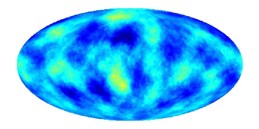
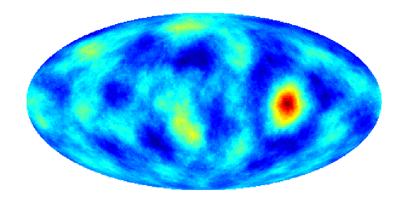
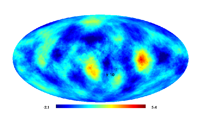
Fig. 3 illustrates how the estimator works for a single randomly generated -like map. We use and take which is similar to the resolution of Planck. In the top panel we show the map (with inner and outer ring radii respectively, as discussed above) associated with a random map. The map associated with the same random which is further lensed by a PIP located at Mpc/h (in the direction of the giant rings ) is shown in the middle panel with no mask and in the bottom panel with the KQ85 mask. As expected the full sky map has a sharper peak than the masked sky.
This indicates that the estimator works as it should. What remains to be done is to repeat this simulation many times and determine the CMB lensing S/N as a function of . Fig. 4 presents the outcome of this process. The confidence level (in terms of standard deviations) for the detection of a PIP with calibrated as discussed above via CMB weak lensing is shown as a function of its distance from us.
We see that in the bulk flow region the CMB lensing is fairly high even with the mask, , whereas for larger it drops. We expect this to be true regardless of the exact profile . This implies that if a PIP is responsible both for the giant rings and for the bulk flow then we should be able to further test the model with CMB weak lensing. However if the giant rings are generated by the PIP and the bulk flow is not, then it is unlikely that its CMB lensing signal is detectable.
Acknowledgements
We thank A. Ben-David, A. Fialkov and E. Kovetz for discussions. We acknowledge the use of the Legacy Archive for Microwave Background Data Analysis (LAMBDA) [18] and the use of the HEALPix package [19]. This work is supported in part by the Israel Science Foundation (grant number 1362/08) and by the European Research Council (grant number 203247).
References
- [1] C. J. Copi, D. Huterer, D. J. Schwarz and G. D. Starkman, Adv. Astron. 2010, 847541 (2010) [arXiv:1004.5602 [astro-ph.CO]].
- [2] C. L. Bennett et al., Astrophys. J. Suppl. 192, 17 (2011) [arXiv:1001.4758 [astro-ph.CO]].
- [3] E. D. Kovetz, A. Ben-David, N. Itzhaki, Astrophys. J. 724, 374-378 (2010). [arXiv:1005.3923 [astro-ph.CO]].
- [4] A. Fialkov, N. Itzhaki, E. D. Kovetz, JCAP 1002, 004 (2010). [arXiv:0911.2100 [astro-ph.CO]].
- [5] D. Sarkar, H. A. Feldman and R. Watkins, Mon. Not. Roy. Astron. Soc. 375, 691 (2007) [astro-ph/0607426].
- [6] H. A. Feldman, M. J. Hudson and R. Watkins, arXiv:0805.1721 [astro-ph].
- [7] R. Watkins, H. A. Feldman and M. J. Hudson, Mon. Not. Roy. Astron. Soc. 392, 743 (2009) [arXiv:0809.4041 [astro-ph]].
- [8] H. A. Feldman, R. Watkins and M. J. Hudson, Mon. Not. Roy. Astron. Soc. 407, 2328 (2010) [arXiv:0911.5516 [astro-ph.CO]].
- [9] S. J. Turnbull, M. J. Hudson, H. A. Feldman, M. Hicken, R. P. Kirshner and R. Watkins, arXiv:1111.0631 [astro-ph.CO].
- [10] N. Itzhaki, JHEP 0810, 061 (2008). [arXiv:0807.3216 [hep-th]].
- [11] N. Itzhaki and E. D. Kovetz, JHEP 0710, 054 (2007) [arXiv:0708.2798 [hep-th]].
- [12] S. Das, D. N. Spergel, Phys. Rev. D79, 043007 (2009). [arXiv:0809.4704 [astro-ph]].
- [13] I. Masina, A. Notari, JCAP 0907, 035 (2009). [arXiv:0905.1073 [astro-ph.CO]].
- [14] I. Masina, A. Notari, JCAP 1009, 028 (2010). [arXiv:1007.0204 [astro-ph.CO]].
- [15] B. Rathaus, A. Fialkov, N. Itzhaki, JCAP 1106, 033 (2011). [arXiv:1105.2940 [astro-ph.CO]].
- [16] A. Nusser and M. Davis, Astrophys. J. 736, 93 (2011) [arXiv:1101.1650 [astro-ph.CO]].
- [17] D. -C. Dai, W. H. Kinney and D. Stojkovic, JCAP 1004, 015 (2011) [arXiv:1102.0800 [astro-ph.CO]].
- [18] http://lambda.gsfc.nasa.gov/
- [19] K. M. Gorski, E. Hivon, A. J. Banday, B. D. Wandelt, F. K. Hansen, M. Reinecke and M. Bartelman, Astrophys. J. 622, 759 (2005) [arXiv:astro-ph/0409513].