Support Vector Regression for Right Censored Data^T1

Yair Goldberglabel=e1]ygoldberg@stat.haifa.ac.il Email: [ Michael R. Kosoroklabel=e2]kosorok@unc.edu Email: [ Affiliation: University of Haifa and The University of North Carolina at Chapel Hill Address: Yair Goldberg
Department of Statistics
The University of Haifa
Mount Carmel, Haifa 31905, Israel Address: Michael R. Kosorok
Department of Biostatistics
The University of North Carolina at Chapel Hill
Chapel Hill, NC 27599, U.S.A.

Abstract

We develop a unified approach for classification and regression support vector machines for data subject to right censoring. We provide finite sample bounds on the generalization error of the algorithm, prove risk consistency for a wide class of probability measures, and study the associated learning rates. We apply the general methodology to estimation of the (truncated) mean, median, quantiles, and for classification problems. We present a simulation study that demonstrates the performance of the proposed approach.

Keywords:

universal consistency,

keywords

[class=AMS]

keywords

^†^†email: e1^†^†email: e2

\setattribute

tablecaptionshape \setattributetablename skip. \arxiv1202.5130

T1The authors are grateful to anonymous associate editor for the helpful suggestions and comments. The authors thank Danyu Lin for many helpful discussions and suggestions. The first author was funded in part by a Gillings Innovation Laboratory (GIL) award at the UNC Gillings School of Global Public Health. The second author was funded in part by NCI grant CA142538.

and

1 Introduction

In many medical studies, estimating the failure time distribution function, or quantities that depend on this distribution, as a function of patient demographic and prognostic variables, is of central importance for risk assessment and health planing. Frequently, such data is subject to right censoring. The goal of this paper is to develop tools for analyzing such data using machine learning techniques.

Traditional approaches to right censored failure time analysis include using parametric models, such as the Weibull distribution, and semiparametric models such as proportional hazard models (see Lawless, 2003, for both). Even when less stringent models—such as nonparametric estimation—are used, it is typically assumed that the distribution function is smooth in both time and covariates (Dabrowska, 1987; Gonzalez-Manteiga and Cadarso-Suarez, 1994). These assumptions seem restrictive, especially when considering today’s high-dimensional data settings.

In this paper, we propose a support vector machine (SVM) learning method for right censored data. The choice of SVM is motivated by the fact that SVM learning methods are easy-to-compute techniques that enable estimation under weak or no assumptions on the distribution (Steinwart and Chirstmann, 2008). SVM learning methods, which we review in detail in Section 2, are a collection of algorithms that attempt to minimize the risk with respect to some loss function. An SVM learning method typically minimizes a regularized version of the empirical risk over some reproducing kernel Hilbert space (RKHS). The resulting minimizer is referred to as the SVM decision function. The SVM learning method is the mapping that assigns to each data set its corresponding SVM decision function.

We adapt the SVM framework to right censored data as follows. First, we represent the distribution’s quantity of interest as a Bayes decision function, i.e., a function that minimizes the risk with respect to a loss function. We then construct a data-dependent version of this loss function using inverse-probability-of-censoring weighting (Robins et al., 1994). We then minimize a regularized empirical risk with respect to this data-dependent loss function to obtain an SVM decision function for censored data. Finally, we define the SVM learning method for censored data as the mapping that assigns for every censored data set its corresponding SVM decision function.

Note that unlike the standard SVM decision function, the proposed censored SVM decision function is obtained as the minimizer of a data-dependent loss function. In other words, for each data set, a different minimization loss function is defined. Moreover, minimizing the empirical risk no longer consists of minimizing a sum of i.i.d. observations. Consequently, different techniques are needed to study the theoretical properties of the censored SVM learning method.

We prove a number of theoretical results for the proposed censored SVM learning method. We first prove that the censored SVM decision function is measurable and unique. We then show that the censored SVM learning method is a measurable learning method. We provide a probabilistic finite-sample bound on the difference in risk between the learned censored SVM decision function and the Bayes risk. We further show that the SVM learning method is consistent for every probability measure for which the censoring is independent of the failure time given the covariates, and the probability that no censoring occurs is positive given the covariates. Finally, we compute learning rates for the censored SVM learning method. We also provide a simulation study that demonstrates the performance of the proposed censored SVM learning method. Our results are obtained under some conditions on the approximation RKHS and the loss function, which can be easily verified. We also assume that the estimation of censoring probability at the observed points is consistent.

We note that a number of other learning algorithms have been suggested for survival data. Biganzoli et al. (1998) and Ripley and Ripley (2001) used neural networks. Segal (1988), Hothorn et al. (2004), Ishwaran et al. (2008), and Zhu and Kosorok (2011), among others, suggested versions of splitting trees and random forests for survival data. Johnson et al. (2004), Shivaswamy et al. (2007), Shim and Hwang (2009), and Zhao et al. (2011), among others, suggested versions of SVM different from the proposed censored SVM. The theoretical properties of most of these algorithms have never been studied. Exceptions include the consistency proof of Ishwaran and Kogalur (2010) for random survival trees, which requires the assumption that the feature space is discrete and finite. In the context of multistage decision problems, Goldberg and Kosorok (2012b) proposed a Q-learning algorithm for right censored data for which a theoretical justification is given, under the assumption that the censoring is independent of both failure time and covariates. However, both of these theoretically justified algorithms are not SVM learning methods. Therefore, we believe that the proposed censored SVM and the accompanying theoretical evaluation given in this paper represent a significant innovation in developing methodology for learning in survival data.

Although the proposed censored SVM approach enables the application of the full SVM framework to right censored data, one potential drawback is the need to estimate the censoring probability at observed failure times. This estimation is required in order to use inverse-probability-of-censoring weighting for constructing the data-dependent loss function. We remark that in many applications it is reasonable to assume that the censoring mechanism is simpler than the failure-time distribution; in these cases, estimation of the censoring distribution is typically easier than estimation of the failure distribution. For example, the censoring may depend only on a subset of the covariates, or may be independent of the covariates; in the latter case, an efficient estimator exists. Moreover, when the only source of censoring is administrative, in other words, when the data is censored because the study ends at a prespecified time, the censoring distribution is often known to be independent of the covariates. Fortunately, the results presented in this paper hold for any censoring estimation technique. We present results for both correctly specified and misspecified censoring models. We also discuss in detail the special cases of the Kaplan-Meier and the Cox model estimators (Fleming and Harrington, 1991).

While the main contribution of this paper is the proposed censored SVM learning method and the study of its properties, an additional contribution is the development of a general machine learning framework for right censored data. The principles and definitions that we discuss in the context of right censored data, such as learning methods, measurability, consistency, and learning rates, are independent of the proposed SVM learning method. This framework can be adapted to other learning methods for right censored data, as well as for learning methods for other missing data mechanisms.

The paper is organized as follows. In Section 2 we review right-censored data and SVM learning methods. In Section 3 we briefly discuss the use of SVM for right-censored data when no censoring is present. Section 4 discusses the difficulties that arise when applying SVM to right censored data and presents the proposed censored SVM learning method. Section 5 contains the main theoretical results, including finite sample bounds and consistency. Simulations appear in Section 6. Concluding remarks appear in Section 7. The lengthier key proofs are provided in the Appendix. Finally, the Matlab code for both the algorithm and the simulations can be found in .

2 Preliminaries

In this section, we establish the notation used throughout the paper. We begin by describing the data setup (Section 2.1). We then discuss loss functions (Section 2.2). Finally we discuss SVM learning methods (Section 2.3). The notation for right censored data generally follows Fleming and Harrington (1991) (6, hereafter abbreviated). For the loss function and the SVM definitions, we follow Steinwart and Chirstmann (2008) (24, hereafter abbreviated).

2.1 Data Setup

We assume the data consist of $n$ independent and identically-distributed random triplets $D=\{(Z_{1},U_{1},\delta_{1}),\ldots,(Z_{n},U_{n},\delta_{n})\}$ . The random vector $Z$ is a covariate vector that takes its values in a set $\mathcal{Z}\subset\mathbb{R}^{d}$ . The random variable $U$ is the observed time defined by $U=T\wedge C$ , where $T\geq 0$ is the failure time, $C$ is the censoring time, and where $a\wedge b=\min(a,b)$ . The indicator $\delta=\bm{1}{\left\{T\leq C\right\}}$ is the failure indicator, where $\bm{1}{\left\{A\right\}}$ is $1$ if $A$ is true and $0$ otherwise, i.e., $\delta=1$ whenever a failure time is observed.

Let $S(t|Z)=P(T>t|Z)$ be the survival functions of $T$ , and let $G(t|Z)=P(C>t|Z)$ be the survival function of $C$ . We make the following assumptions:

(A1)

$C$ takes its values in the segment $[0,\tau]$ for some finite $\tau>0$ , and $\inf_{z\in\mathcal{Z}}G(\tau-|z)\geq 2K>0$ .
(A2)

$C$ is independent of $T$ , given $Z$ .

The first assumption assures that there is a positive probability of censoring over the observation time range ( $[0,\tau]$ ). Note that the existence of such a $\tau$ is typical since most studies have a finite time period of observation. In the above, we also define $F(t-)$ to be the left-hand limit of a right continuous function $F$ with left-hand limits. The second assumption is standard in survival analysis and ensures that the joint nonparametric distribution of the survival and censoring times, given the covariates, is identifiable.

We assume that the censoring mechanism can be described by some simple model. Below, we consider two possible examples, although the main results do not require any specific model. First, we need some notation. For every $t\in[0,\tau]$ , define $\mathbf{N}(t)=\bm{1}{\left\{U\leq t,\delta=0\right\}}$ and $\mathbf{Y}(t)=\bm{1}{\left\{U>t\right\}}+\bm{1}{\left\{U=t,\delta=0\right\}}$ . Note that since we are interested in the survival function of the censoring variable, $\mathbf{N}(t)$ is the counting process for the censoring, and not for the failure events, and $\mathbf{Y}(t)$ is the at-risk process for observing a censoring time. For a cadlag function $A$ on $(0,\tau]$ , define the product integral $\phi(A)(t)=\prod_{0<s\leq t}(1+dA(s))$ (van der Vaart and Wellner, 1996). Define $\mathbb{P}_{n}$ to be the empirical measure, i.e., $\mathbb{P}_{n}f(X)=n^{-1}\sum_{i=1}^{n}f(X_{i})$ . Define $Pf$ to be the expectation of $f$ with respect to $P$ .

Example 1.

Independent censoring: Assume that $C$ is independent of both $T$ and $Z$ . Define

\displaystyle\hat{\Lambda}(t)=\int_{0}^{t}\frac{\mathbb{P}_{n}d\mathbf{N}(s)}{\mathbb{P}_{n}\mathbf{Y}(s)}\,.

Then $\hat{G}_{n}(t)=\phi(-\hat{\Lambda})(t)$ is the Kaplan-Meier estimator for $G$ . $\hat{G}_{n}$ is a consistent and efficient estimator for the survival function $G$ (6).

Example 2.

The proportional hazards model: Consider the case that the hazard of $C$ give $Z$ is of the form $e^{Z^{\prime}{\bm{\beta}}}d\Lambda$ for some unknown vector ${\bm{\beta}}\in\mathbb{R}^{d}$ and some continuous unknown nondecreasing function $\Lambda$ with $\Lambda(0)=0$ and $0<\Lambda(\tau)<\infty$ . Let $\hat{{\bm{\beta}}}$ be the zero of the estimating equation

\displaystyle\Phi_{n}({\bm{\beta}})=\mathbb{P}_{n}\int_{0}^{\tau}\left(Z-\frac{\mathbb{P}_{n}Z\mathbf{Y}(s)e^{{\bm{\beta}}^{\prime}Z}}{\mathbb{P}_{n}\mathbf{Y}(s)e^{{\bm{\beta}}^{\prime}Z}}\right)d\mathbf{N}(s)\,.

Define

\displaystyle\hat{\Lambda}(t)=\int_{0}^{t}\frac{\mathbb{P}_{n}d\mathbf{N}(s)}{\mathbb{P}_{n}\mathbf{Y}(s)e^{\hat{\bm{\beta}}^{\prime}Z}}\,.

Then $\hat{G}_{n}(t|z)=\phi(-e^{\hat{\bm{\beta}}^{\prime}z}\hat{\Lambda}(t))$ is a consistent and efficient estimator for survival function $G$ (6).

Even when no simple form for the censoring mechanism is assumed, the censoring distribution can be estimated using a generalization of the Kaplan-Meier estimator of Example 1.

Example 3.

Generalized Kaplan-Meier: Let $k_{\sigma}:\mathcal{Z}\times Z\mapsto\mathbb{R}$ be a kernel function of width $\sigma$ . Define $\hat{\mathbf{N}}(t,z)=K(z,Z)\bm{1}{\left\{U\leq t,\delta=0\right\}}$ and $\hat{\mathbf{Y}}(t,z)=K(z,Z)(\bm{1}{\left\{U>t\right\}}+\bm{1}{\left\{U=t,\delta=0\right\}})$ . Define

\displaystyle\hat{\Lambda}(t|z)=\int_{0}^{t}\frac{\mathbb{P}_{n}d\hat{\mathbf{N}}(s,z)}{\mathbb{P}_{n}\mathbf{Y}(s,z)}\,.

Then the generalized Kaplan-Meier estimator is given by $\hat{G}_{n}(t|z)=\phi(-\hat{\Lambda})(t|z)$ , where the product integral $\phi$ is defined for every fixed $z$ . Under some conditions, Dabrowska (1987); Dabrowska (1989) proved consistency of the estimator and discussed its convergence rates.

Usually we denote the estimator of the survival function of the censoring variable $G(t|Z)$ by $\hat{G}_{n}(t|Z)$ without referring to a specific estimation method. When needed, the specific estimation method will be discussed. When independent censoring is assumed, as in Example 1, we denote the estimator by $\hat{G}_{n}(t)$ .

Remark 4.

By Assumption (A1), $\inf_{z\in\mathcal{Z}}G(\tau|z)\geq 2K>0$ , and thus if the estimator $\hat{G}_{n}$ is consistent for $G$ , then, for all $n$ large enough, $\inf_{z\in\mathcal{Z}}\hat{G}_{n}(\tau|z)>K>0$ . In the following, for simplicity, we assume that the estimator $\hat{G}_{n}$ is such that $\inf_{Z}\hat{G}_{n}(\tau|Z)>K>0$ . In general, one can always replace $\hat{G}_{n}$ by $\hat{G}_{n}\vee K_{n}$ , where $K_{n}\rightarrow 0$ . In this case, for all $n$ large enough, $\inf_{Z}\hat{G}_{n}(\tau|Z)>K>0$ and for all $n$ , $\inf\hat{G}_{n}>0$ .

2.2 Loss Functions

Let the input space $(\mathcal{Z},\mathcal{A})$ be a measurable space. Let the response space $\mathcal{Y}$ be a closed subset of $\mathbb{R}$ . Let $P$ be a measure on $\mathcal{Z}\times\mathcal{Y}$ .

A function $L:\mathcal{Z}\times\mathcal{Y}\times\mathbb{R}\mapsto[0,\infty)$ is a loss function if it is measurable. We say that a loss function $L$ is convex if $L(z,y,\cdot)$ is convex for every $z\in\mathcal{Z}$ and $y\in\mathcal{Y}$ . We say that a loss function $L$ is locally Lipschitz continuous with Lipschitz local constant function $c_{L}(\cdot)$ if for every $a>0$

\displaystyle\sup_{\begin{subarray}{c}z\in\mathcal{Z}\\ y\in\mathcal{Y}\end{subarray}}|L(z,y,s)-L(z,y,s^{\prime})|<c_{L}(a)|s-s^{\prime}|\,,\quad s,s^{\prime}\in[-a,a]\,.

We say that $L$ is Lipschitz continuous if there is a constant $c_{L}$ such that the above holds for any $a$ with $c_{L}(a)=c_{L}$ .

For any measurable function $f:\mathcal{Z}\mapsto\mathbb{R}$ we define the $L$ -risk of $f$ with respect to the measure $P$ as $\mathcal{R}_{L,P}(f)=E_{P}[L(Z,Y,f(Z))]$ . We define the Bayes risk $\mathcal{R}^{*}_{L,P}$ of $f$ with respect to loss function $L$ and measure $P$ as $\inf_{f}\mathcal{R}_{L,P}(f)$ , where the infimum is taken over all measurable functions $f:\mathcal{Z}\mapsto\mathbb{R}$ . A function $f^{*}_{L,P}$ that achieves this infimum is called a Bayes decision function.

We now present a few examples of loss functions and their respective Bayes decision functions. In the next section we discuss the use of these loss functions for right censored data.

Example 5.

Binary classification: Assume that $\mathcal{Y}=\{-1,1\}$ . We would like to find a function $f:\mathcal{Z}\mapsto\{-1,1\}$ such that for almost every $z$ , $P(f(z)=Y|Z=z)\geq 1/2$ . One can think of $f$ as a function that predicts the label $y$ of a pair $(z,y)$ when only $z$ is observed. In this case, the desired function is the Bayes decision function $f^{*}_{L,P}$ with respect to the loss function $L_{\mathrm{BC}}(z,y,s)=\bm{1}{\left\{y\cdot\mathrm{sign}(s)\neq 1\right\}}$ . In practice, since the loss function $L_{\mathrm{BC}}$ is not convex, it is usually replaced by the hinge loss function $L_{\mathrm{HL}}(z,y,s)=\max\{0,1-ys\}$ .

Example 6.

Expectation: Assume that $\mathcal{Y}=\mathbb{R}$ . We would like to estimate the expectation of the response $Y$ given the covariates $Z$ . The conditional expectation is the Bayes decision function $f^{*}_{L,P}$ with respect to the squared error loss function $L_{\mathrm{LS}}(z,y,s)=(y-s)^{2}$ .

Example 7.

Median and quantiles: Assume that $\mathcal{Y}=\mathbb{R}$ . We would like to estimate the median of $Y|Z$ . The conditional median is the Bayes decision function $f^{*}_{L,P}$ for the absolute deviation loss function $L_{\mathrm{AD}}(z,y,s)=|y-s|$ . Similarly, the $\alpha$ -quantile of $Y$ given $Z$ is obtained as the Bayes decision function for the loss function

\displaystyle L_{\alpha}(z,y,s)=\left\{\begin{array}[]{ll}-(1-\alpha)(y-s)&\mathrm{if\,}s\geq y\\ \alpha(y-s)&\mathrm{if\,}s<y\\ \end{array}\right.\quad,\;\alpha\in(0,1)\,.

Note that the functions $L_{\mathrm{HL}}$ , $L_{\mathrm{LS}}$ , $L_{\mathrm{AD}}$ , and $L_{\alpha}$ for $\alpha\in(0,1)$ are all convex. Moreover, all these functions except $L_{\mathrm{LS}}$ are Lipschitz continuous, and $L_{\mathrm{LS}}$ is locally Lipschitz continuous when $\mathcal{Y}$ is compact.

2.3 Support Vector Machine (SVM) Learning Methods

Let $L$ be a convex locally Lipschitz continuous loss function. Let $H$ be a separable reproducing kernel Hilbert space (RKHS) of a bounded measurable kernel on $\mathcal{Z}$ (for details regarding RKHS, the reader is referred to 24, Chapter 4).

Let $D_{0}=\{(Z_{1},Y_{1}),\ldots,(Z_{n},Y_{n})\}$ be a set of $n$ i.i.d. observations drawn according to the probability measure $P$ . Fix $\lambda$ and let $H$ be as above. Define the empirical SVM decision function

\displaystyle f_{D_{0},\lambda}=\operatornamewithlimits{argmin}_{f\in H}\lambda\|f\|_{H}^{2}+\mathcal{R}_{L,D_{0}}(f)\,,

(1)

where

\displaystyle\mathcal{R}_{L,D_{0}}(f)\equiv\mathbb{P}_{n}L(Z,Y,f(Z))\equiv\frac{1}{n}\sum_{i=1}^{n}L(Z_{i},Y_{i},f(Z_{i}))

is the empirical risk.

For some sequence $\{\lambda_{n}\}$ , define the SVM learning method $\mathfrak{L}$ , as the map

\displaystyle\begin{split}(\mathcal{Z}\times\mathcal{Y})^{n}\times\mathcal{Z}&\mapsto\mathbb{R}\\ (D_{0},z)&\mapsto f_{D_{0},\lambda_{n}}\end{split}

(2)

for all $n\geq 1$ . We say that $\mathfrak{L}$ is measurable if it is measurable for all $n$ with respect to the minimal completion of the product $\sigma$ -field on $(\mathcal{Z}\times\mathcal{Y})^{n}\times\mathcal{Z}$ . We say that that $\mathfrak{L}$ is ( $L$ -risk) $P$ -consistent if for all $\varepsilon>0$

\displaystyle\lim_{n\rightarrow\infty}P(D_{0}\in(Z\times\mathcal{Y})^{n}\,:\,\mathcal{R}_{L,P}(f_{D_{0},\lambda_{n}})\leq\mathcal{R}_{L,P}^{*}+\varepsilon)=1\,.

(3)

We say that $\mathfrak{L}$ is universally consistent if for all distributions $P$ on $\mathcal{Z}\times\mathcal{Y}$ , $\mathfrak{L}$ is $P$ -consistent.

We now briefly summarize some known results regarding SVM learning methods needed for our exposition. More advanced results can be obtained using conditions on the functional spaces and clipping. We will discuss these ideas in the context of censoring in Section 5.

Theorem 8.

Let $L:\mathcal{Z}\times\mathcal{Y}\times\mathbb{R}\mapsto[0,\infty)$ be a convex Lipschitz continuous loss function such that $L(z,y,0)$ is uniformly bounded. Let $H$ be a separable RKHS of a bounded measurable kernel on the set $\mathcal{Z}\subset\mathbb{R}^{d}$ . Choose $0<\lambda_{n}<1$ such that $\lambda_{n}\rightarrow 0$ , and $\lambda_{n}^{2}n\rightarrow\infty$ . Then

(a)

The empirical SVM decision function $f_{D_{0},\lambda_{n}}$ exists and is unique.
(b)

The SVM learning method $\mathfrak{L}$ defined in (2) is measurable.
(c)

The $L$ -risk $\mathcal{R}_{L,P}(f_{D_{0},\lambda_{n}})\stackrel{{\scriptstyle\mbox{\scriptsize\rm P}}}{{\rightarrow}}\inf_{f\in H}\mathcal{R}_{L,P}(f)$ .
(d)

If the RKHS $H$ is dense in the set of integrable functions on $\mathcal{Z}$ , then the SVM learning method $\mathfrak{L}$ is universally consistent.

The proof of (a) follows from 24, Lemma 5.1 and Theorem 5.2. For the proof of (b), see 24, Lemma 6.23. The proof of (c) follows from 24 Theorem 6.24. The proof of (d) follows from 24, Theorem 5.31, together with Theorem 6.24.

3 SVM for Survival Data without Censoring

In this section we present a few examples of the use of SVM for survival data but without censoring. We show how different quantities obtained from the conditional distribution of $T$ given $Z$ can be represented as Bayes decision functions. We then show how SVM learning methods can be applied to these estimation problems and briefly review theoretical properties of such SVM learning methods. In the next section we will explain why these standard SVM techniques cannot be employed directly when censoring is present.

Let $(Z,T)$ be a random vector where $Z$ is a covariate vector that takes its values in a set $\mathcal{Z}\subset\mathbb{R}^{d}$ , $T$ is survival time that takes it values in $\mathcal{T}=[0,\tau]$ for some positive constant $\tau$ , and where $(Z,T)$ is distributed according to a probability measure $P$ on $\mathcal{Z}\times\mathcal{T}$ .

Note that the conditional expectation $P[T|Z]$ is the Bayes decision function for the least squares loss function $L_{\mathrm{LS}}$ . In other words

\displaystyle P[T|Z]=\operatornamewithlimits{argmin}_{f}P[L_{\mathrm{LS}}(Z,T,f(Z))]\,,

where the minimization is taken over all measurable real functions on $\mathcal{Z}$ (see Example 6). Similarly, the conditional median and the $\alpha$ -quantile of $T|Z$ can be shown to be the Bayes decision functions for the absolute deviation function $L_{\mathrm{AD}}$ and $L_{\alpha}$ , respectively (see Example 7). In the same manner, one can represent other quantities of the conditional distribution $T|Z$ using Bayes decision functions.

Defining quantities computed from the survival function as Bayes decision functions is not limited to regression (i.e., to a continuous response). Classification problems can also arise in the analysis of survival data (Ripley and Ripley, 2001; Johnson et al., 2004, see, for example,). For example, let $\rho$ , $0<\rho<\tau$ , be a cutoff constant. Assume that survival to a time greater than $\rho$ is considered as death unrelated to the disease (i.e., remission) and a survival time less than or equal to $\rho$ is considered as death resulting from the disease. Denote

\displaystyle Y(T)=\left\{\begin{array}[]{cc}1&T>\rho\\ -1&T\leq\rho\\ \end{array}\right.\,.

In this case, the decision function that predicts remission when the probability of $Y=1$ given the covariates is greater than $1/2$ and failure otherwise is a Bayes decision function for the binary classification loss $L_{\mathrm{BC}}$ of Example 5.

Let $D_{0}=\{(Z_{1},T_{1}),\ldots,(Z_{n},T_{n})\}$ be a data set of $n$ i.i.d. observations distributed according to $P$ . Let $Y_{i}=Y(T_{i})$ where $Y(\cdot):\mathcal{T}\mapsto\mathcal{Y}$ is some deterministic measurable function. For regression problems, $Y$ is typically the identity function and for classification $Y$ can be defined, for example, as in (3). Let $L$ be a convex locally Lipschitz continuous loss function, $L:\mathcal{Z}\times\mathcal{Y}\times\mathbb{R}\mapsto[0,\infty)$ . Note that this includes the loss functions $L_{\mathrm{LS}},L_{\mathrm{AD}}$ , $L_{\alpha}$ , and $L_{\mathrm{HL}}$ . Define the empirical decision function as in (1) and the SVM learning method $\mathfrak{L}$ as in (2). Then it follows from Theorem 8 that for an appropriate RKHS $H$ and regularization sequence $\{\lambda_{n}\}$ , $\mathfrak{L}$ is measurable and universally consistent.

4 Censored SVM

In the previous section, we presented a few examples of the use of SVM for survival data without censoring. In this section we explain why standard SVM techniques cannot be applied directly when censoring is present. We then explain how to use inverse probability of censoring weighting (Robins et al., 1994) to obtain a censored SVM learning method. Finally, we show that the obtained censored SVM learning method is well defined.

Let $D=\{(Z_{1},U_{1},\delta_{1}),\ldots,(Z_{n},U_{n},\delta_{n})\}$ be a set of $n$ i.i.d. random triplets of right censored data (as described in Section 2.1). Let $L:Z\times\mathcal{Y}\times\mathbb{R}\mapsto[0,\infty)$ be a convex locally Lipschitz loss function. Let $H$ be a separable RKHS of a bounded measurable kernel on $\mathcal{Z}$ . We would like to find an empirical SVM decision function. In other words, we would like to find the minimizer of

\displaystyle\lambda\|f\|_{H}^{2}+\mathcal{R}_{L,D}(f)\equiv\lambda\|f\|_{H}^{2}+\frac{1}{n}\sum_{i=1}^{n}L(Z_{i},Y(T_{i}),f(Z_{i}))

(6)

where $\lambda>0$ is a fixed constant, and $Y:\mathcal{T}\mapsto\mathcal{Y}$ is a known function. The problem is that the failure times $T_{i}$ may be censored, and thus unknown. While a simple solution is to ignore the censored observations, it is well known that this can lead to severe bias (Tsiatis, 2006).

In order to avoid this bias, one can reweight the uncensored observations. Note that at time $T_{i}$ , the $i$ -th observation has probability $G(T_{i}-|Z_{i})\equiv P(C_{i}\geq T_{i}|Z_{i})$ not to be censored, and thus, one can use the inverse of the censoring probability for reweighting in (6) (Robins et al., 1994).

More specifically, define the random loss function $L^{n}:(\mathcal{Z}\times\mathcal{T}\times\{0,1\})^{n}\times(\mathcal{Z}\times\mathcal{T}\times\{0,1\}\times\mathbb{R})\mapsto\mathbb{R}$ by

\displaystyle L^{n}(D,(z,u,\delta,s))=\left\{\begin{array}[]{cc}\frac{L(z,Y(u),s)}{\hat{G}_{n}(u|z)},&\delta=1,\\ 0,&\delta=0,\\ \end{array}\right.

where $\hat{G}_{n}$ is the estimator of the survival function of the censoring variable based on the set of $n$ random triplets $D$ (see Section 2.1). When $D$ is given, we denote $L^{n}_{D}(\cdot)\equiv L^{n}(D,\cdot)$ . Note that in this case the function $L^{n}_{D}$ is no longer random. In order to show that $L^{n}_{D}$ is a loss function, we need to show that $L^{n}_{D}$ is a measurable function.

Lemma 9.

Let $L$ be a convex locally Lipschitz loss function. Assume that the estimation procedure $D\mapsto\hat{G}_{n}(\cdot|\cdot)$ is measurable. Then for every $D\in(\mathcal{Z}\times\mathcal{T}\times\{0,1\})^{n}$ the function $L^{n}_{D}:(\mathcal{Z}\times\mathcal{T}\times\{0,1\})\times\mathbb{R}\mapsto\mathbb{R}$ is measurable.

Proof.

By Remark 4, the function $\hat{G}_{n}(u|z)\mapsto 1/\hat{G}_{n}(u|z)$ is well defined. Since by definition, both $Y$ and $L$ are measurable, we obtain that $(u,z,\delta)\mapsto\delta L(Y(u),z)/\hat{G}_{n}(u|z)$ is measurable. ∎

We define the empirical censored SVM decision function to be

\displaystyle f^{c}_{D,\lambda}=\operatornamewithlimits{argmin}_{f\in H}\lambda\|f\|_{H}^{2}+\mathcal{R}_{L^{n}_{D},D}(f)\equiv\operatornamewithlimits{argmin}_{f\in H}\lambda\|f\|_{H}^{2}+\frac{1}{n}\sum L^{n}_{D}\big(Z_{i},U_{i},\delta_{i},f(Z_{i})\big)\,.

(7)

The existence and uniqueness of the empirical censored SVM decision function is ensured by the following lemma:

Lemma 10.

Let $L$ be a convex locally Lipschitz loss function. Let $H$ be a separable RKHS of a bounded measurable kernel on $\mathcal{Z}$ . Then there exists a unique empirical censored SVM decision function.

Proof.

Note that given $D$ , the loss function $L^{n}_{D}(z,u,\delta,\cdot)$ is convex for every fixed $z$ , $u$ , and $\delta$ . Hence, the result follows from Lemma 5.1 together with Theorem 5.2 of 24. ∎

Note that the empirical censored SVM decision function is just the empirical SVM decision function of (1), after replacing the loss function $L$ with the loss function $L^{n}_{D}$ . However, there are two important implications to this replacement. Firstly, empirical censored SVM decision functions are obtained by minimizing a different loss function for each given data set. Secondly, the second expression in the minimization problem (7), namely,

\displaystyle\mathcal{R}_{L^{n}_{D},D}(f)\equiv\frac{1}{n}\sum_{i=1}^{n}L^{n}_{D}\big(Z_{i},U_{i},\delta_{i},f(Z_{i})\big),

is no longer constructed from a sum of i.i.d. random variables.

We would like to show that the learning method defined by the empirical censored SVM decision functions is indeed a learning method. We first define the term learning method for right censored data or censored learning method for short.

Definition 11.

A censored learning method $\mathfrak{L}^{c}$ on $\mathcal{Z}\times\mathcal{T}$ maps every data set $D\in(\mathcal{Z}\times\mathcal{T}\times\{0,1\})^{n}$ , $n\geq 1$ , to a function $f_{D}:\mathcal{Z}\mapsto\mathbb{R}$ .

Choose $0<\lambda_{n}<1$ such that $\lambda_{n}\rightarrow 0$ . Define the censored SVM learning method $\mathfrak{L}^{c}$ , as $\mathfrak{L}^{c}(D)=f^{c}_{D,\lambda_{n}}$ for all $n\geq 1$ . The measurability of the censored SVM learning method $\mathfrak{L}^{c}$ is ensured by the following lemma, which is an adaptation of Lemma 6.23 of 24 to the censored case.

Lemma 12.

Let $L$ be a convex locally Lipschitz loss function. Let $H$ be a separable RKHS of a bounded measurable kernel on $\mathcal{Z}$ . Assume that the estimation procedure $D\mapsto\hat{G}_{n}(\cdot|\cdot)$ is measurable. Then the censored SVM learning method $\mathfrak{L}^{c}$ is measurable, and the map $D\mapsto f^{c}_{D,\lambda_{n}}$ is measurable.

Proof.

First, by Lemma 2.11 of 24, for any $f\in H$ , the map $(z,u,f)\mapsto L(z,Y(u),f(z))$ is measurable. The survival function $\hat{G}_{n}$ is measurable on $(\mathcal{Z}\times\mathbb{R}\times\{0,1\})^{n}\times(\mathcal{Z}\times\mathbb{R})$ and by Remark 4, the function $D\mapsto\delta_{i}/\hat{G}_{n}(u_{i}|z_{i})$ is well defined and measurable. Hence $D\mapsto n^{-1}\sum_{i=1}^{n}\frac{\delta_{i}L(z_{i},Y(u_{i}),f(z_{i}))}{\hat{G}_{n}(u_{i}|z_{i})}$ is measurable. Note that the map $f\mapsto\lambda_{n}\|f\|_{H}^{2}$ where $f\in H$ is also measurable. Hence we obtain that the map $\phi:(\mathcal{Z}\times\mathcal{T}\times\{0,1\})^{n}\times H\mapsto\mathbb{R}$ , defined by

\displaystyle\phi(D,f)=\lambda\|f\|_{H}^{2}+\mathcal{R}_{L^{n}_{D},D}(f)\,,

is measurable. By Lemma 10, $f^{c}_{D,\lambda_{n}}$ is the only element of $H$ satisfying

\displaystyle\phi(D,f^{c}_{D,\lambda_{n}})=\inf_{f\in H}\phi(D,f)\,.

By Aumann’s measurable selection principle (24, Lemma A.3.18), the map $D\mapsto f^{c}_{D,\lambda_{n}}$ is measurable with respect to the minimal completion of the product $\sigma$ -field on $(\mathcal{Z}\times\mathcal{T}\times\{0,1\})^{n}$ . Since the evaluation map $(f,z)\mapsto f(z)$ is measurable (24, Lemma 2.11), the map $(D,z)\mapsto f^{c}_{D,\lambda_{n}}(z)$ is also measurable. ∎

5 Theoretical Results

In the following, we discuss some theoretical results regarding the censored SVM learning method proposed in Section 4. In Section 5.1 we discuss function clipping which will serve as a tool in our analysis. In Section 5.2 we discuss finite sample bounds. In Section 5.3 we discuss consistency. Learning rates are discussed in Section 5.4. Finally, censoring model misspecification is discussed in Section 5.5.

5.1 Clipped Censored SVM Learning Method

In order to establish the theoretical results of this section we first need to introduce the concept of clipping. We say that a loss function $L$ can be clipped at $M>0$ , if, for all $(z,y,s)\in\mathcal{Z}\times\mathcal{Y}\times\mathbb{R}$ ,

\displaystyle L(z,y,\accentset{\frown}{s})\leq L(z,y,s)

where $\accentset{\frown}{s}$ denotes the clipped value of $s$ at $\pm M$ , that is,

\displaystyle\accentset{\frown}{s}=\left\{\begin{array}[]{cl}-M&\quad\text{if }s\leq-M\\ s&\quad\text{if }-M<s<M\\ M&\quad\text{if }s\geq M\\ \end{array}\right.

(see 24, Definition 2.22). The loss functions $L_{\mathrm{HL}}$ , $L_{\mathrm{LS}}$ , $L_{\mathrm{AD}}$ , and $L_{\alpha}$ can be clipped at some $M$ when $\mathcal{Y}=\mathcal{T}$ or $\mathcal{Y}=\{-1,1\}$ (24, Chapter 2).

In our context the response variable $Y$ usually takes it values in a bounded set (see Section 3). When the response space is bounded, we have the following criterion for clipping. Let $L$ be a distance-based loss function, i.e., $L(z,y,s)=\phi(s-y)$ for some function $\phi$ . Assume that $\lim_{r\rightarrow\pm\infty}\phi(r)=\infty$ . Then $L$ can be clipped at some $M$ (24, Chapter 2).

Moreover, when the sets $\mathcal{Z}$ and $\mathcal{Y}$ are compact, we have the following criterion for clipping which is usually easy to check.

Lemma 13.

Let $\mathcal{Z}$ and $\mathcal{Y}$ be compact. Let $L:\mathcal{Z}\times\mathcal{Y}\times\mathbb{R}\mapsto[0,\infty)$ be continuous and strictly convex, with a bounded minimizer for every $(z,y)\in\mathcal{Z}\times\mathcal{Y}$ . Then $L$ can be clipped at some $M$ .

See proof in Appendix A.3.

For a function $f$ , we define $\accentset{\frown}{f}$ to be the clipped version of $f$ , i.e., $\accentset{\frown}{f}=\max\{-M,\min\{M,f\}\}$ . Finally, we note that the clipped censored SVM learning method, that maps every data set $D\in(\mathcal{Z}\times\mathcal{T}\times\{0,1\})^{n}$ , $n\geq 1$ , to the function $\accentset{\frown}{f}^{c}_{D,\lambda}$ is measurable, where $\accentset{\frown}{f}^{c}_{D,\lambda}$ is the clipped version of $f^{c}_{D,\lambda}$ defined in (7). This follows from Lemma 12, together with the measurability of the clipping operator.

5.2 Finite Sample Bounds

We would like to establish a finite-sample bound for the generalization of clipped censored SVM learning methods. We first need some notation. Define the censoring estimation error

\displaystyle Err_{n}(t,z)=\hat{G}_{n}(t|z)-G(t|z)\,,\qquad(t,z)\in\mathcal{T}\times\mathcal{Z}

to be the difference between the estimated and true survival functions of the censoring variable.

Let $H$ be an RKHS over the covariates space $\mathcal{Z}\subset\mathbb{R}^{d}$ . Define the $n$ -th dyadic entropy number $e_{n}(H,\|\cdot\|_{H})$ as the infimum over $\varepsilon$ , such that $H$ can be covered with no more than $2^{n-1}$ balls of radius $\varepsilon$ with respect to the metric induced by the norm. For a bounded linear transformation $S:H\mapsto F$ where $F$ is a normed space, we define the dyadic entropy number $e_{n}(S)$ as $e_{n}(SB_{H},\|\cdot\|_{F})$ . For details, the reader is referred to Appendix 5.6 of 24.

Define the Bayes risk $\mathcal{R}_{L,P}^{*}=\inf_{f}\mathcal{R}_{L,P}(f)$ , where the infimum is taken over all measurable functions $f:\mathcal{Z}\mapsto\mathbb{R}$ . Note that Bayes risk is defined with respect to both the loss $L$ and the distribution $P$ . When a function $f_{P,L}^{*}$ exists such that $\mathcal{R}_{L,P}(f_{P,L}^{*})=\mathcal{R}_{L,P}^{*}$ we say that $f_{P,L}^{*}$ is a Bayes decision function.

We need the following assumptions:

(B1)

The loss function $L:\mathcal{Z}\times\mathcal{Y}\times\mathbb{R}\mapsto[0,\infty)$ is a locally Lipschitz continuous loss function that can be clipped at $M>0$ such that the supremum bound

$\displaystyle L(z,y,s)\leq B$ (8)

holds for all $z,y,s\in\mathcal{Z}\times\mathcal{Y}\times[-M,M]$ and for some $B>0$ . Moreover, there is a constant $q>0$ such that

$\displaystyle|L(z,y,s)-L(z,y,0)|\leq c|s|^{q}$

for all $z,t,s\in\mathcal{Z}\times\mathcal{Y}\times\mathbb{R}$ and for some $c>0$ .

(B2)

$H$ is a separable RKHS of a measurable kernel over $\mathcal{Z}$ and $P$ is a distribution over $\mathcal{Z}\times\mathcal{T}$ for which there exist constants $\vartheta\in[0,1]$ and $V>B^{2-\vartheta}$ such that

\displaystyle P\left(L\circ\accentset{\frown}{f}-L\circ f_{P,L}^{*}\right)^{2}\leq VP\left(L\circ\accentset{\frown}{f}-L\circ f_{P,L}^{*}\right)^{\vartheta}

(9)

for all $z,y,s\in\mathcal{Z}\times\mathcal{Y}\times[-M,M]$ and $f\in H$ ; and where $L\circ f$ is shorthand for the function $(z,y)\mapsto L(z,y,f(z))$ .

(B3)

There are constants $a>1$ and $0<p<1$ , such that for for all $i\geq 1$ the following entropy bound holds:

$\displaystyle P[e_{i}(\textrm{id}:H\mapsto L_{2}(\mathbb{P}_{n}))]\leq ai^{-\frac{1}{2p}}\,,$ (10)

where $\textrm{id}:H\mapsto L_{2}(\mathbb{P}_{n})$ is the embedding of $H$ into the space of square integrable functions with respect to the empirical measure $\mathbb{P}_{n}$ .

Before we state the main result of this section, we present some examples for which the assumptions above hold:

Remark 14.

When $\mathcal{Y}$ is contained in a compact set, Assumption (B1) holds with $q=1$ for $L_{\mathrm{HL}}$ , $L_{\mathrm{AD}}$ and $L_{\alpha}$ and with $q=2$ for $L_{\mathrm{LS}}$ (recall the definitions of the loss functions from Section 2.2).

Remark 15.

Assumption (B2) holds trivially for $\vartheta=0$ with $V=B^{2}$ . It holds for $L_{\mathrm{LS}}$ with $\vartheta=1$ for compact $\mathcal{Y}$ (24, Example 7.3). Under some conditions on the distribution, it also holds for $L_{\mathrm{AD}}$ and $L_{\alpha}$ (24, Eq. 9.29).

Remark 16.

When $\mathcal{Z}\subset\mathbb{R}^{d}$ is compact, the entropy bound (10) of Assumption (B3) is satisfied for smooth kernels such as the polynomial and Gaussian kernels for all $p>0$ (see 24, Section 6.4). The assumption also holds for Gaussian kernels over $\mathbb{R}^{d}$ for distributions $P_{Z}$ with positive tail exponent (see 24, Section 7.5).

We are now ready to establish a finite sample bound for the clipped censored SVM learning methods:

Theorem 17.

Let $L$ be a loss function and $H$ be an RKHS such that assumptions (B1)–(B3) hold. Let $f_{0}\in H$ satisfy $\|L\circ f_{0}\|_{\infty}\leq B_{0}$ for some $B_{0}\geq B$ . Let $\hat{G}_{n}(t|Z)$ be an estimator of the survival function of the censoring variable and assume (A1)–(A2). Then, for any fixed regularization constant $\lambda>0$ , $n\geq 1$ , and $\eta>0$ , with probability not less than $1-3e^{-\eta}$ ,

	$\displaystyle\lambda\\|f^{c}_{D,\lambda}\\|_{H}^{2}+\mathcal{R}_{L,P}(\accentset{\frown}{f}^{c}_{D,\lambda})-\mathcal{R}_{L,P}^{*}\leq$	$\displaystyle 3(\lambda\\|f_{0}\\|_{H}^{2}+\mathcal{R}_{L,P}(f_{0})-\mathcal{R}_{L,P}^{*})+3\left(\frac{72\tilde{V}\eta}{n}\right)^{1/(2-\vartheta)}$
		$\displaystyle+\frac{8B_{0}\eta}{5Kn}+\frac{3B}{K^{2}}\mathbb{P}_{n}Err_{n}+W\left(\frac{a^{2p}}{\lambda^{p}n}\right)^{\frac{1}{2-p-\vartheta+\vartheta p}}\,,$

where $W$ is a constant that depends only $p$ , $M$ , $B$ , $\vartheta$ , $V$ and $K$ .

The proof appears in Appendix A.2.

For the Kaplan-Meier estimator (see Example 1) bounds of the random error $\|Err_{n}\|_{\infty}$ were established (Bitouzé et al., 1999). In this case we can replace the bound of Theorem 17 with a more explicit one.

Specifically, let $\hat{G}_{n}$ be the Kaplan-Meier estimator. Let $0<K_{S}=P(T\geq\tau)$ be a lower bound on the survival function at $\tau$ . Then, for every $n\geq 1$ and $\varepsilon>0$ the following Dvoretzky-Kiefer-Wolfowitz-type inequality holds (Bitouzé et al., 1999, Theorem 2):

\displaystyle P(\|\hat{G}_{n}-G\|_{\infty}>\varepsilon)

\displaystyle<\frac{5}{2}\exp\{-2nK_{S}^{2}\varepsilon^{2}+D_{o}\sqrt{n}K_{S}\varepsilon\}\,,

where $D_{o}$ is some universal constant (see Wellner, 2007, for a bound on $D_{o}$ ). Some algebraic manipulations then yield (Goldberg and Kosorok, 2013) that for every $\eta>0$ and $n\geq 1$

\displaystyle P\left(\|\hat{G}_{n}-G\|_{\infty}>\frac{\sqrt{2\eta}+D_{o}}{K_{S}\sqrt{n}}\right)

\displaystyle<\frac{5}{2}e^{-\eta}\,.

(11)

As a result, we obtain the following corollary:

Corollary 18.

Consider the setup of Theorem 17. Assume that the censoring variable $C$ is independent of both $T$ and $Z$ . Let $\hat{G}_{n}$ be the Kaplan-Meier estimator of $G$ . Then for any fixed regularization constant $\lambda$ , $n\geq 1$ , and $\eta>0$ , with probability not less than $1-\frac{11}{2}e^{-\eta}$ ,

	$\displaystyle\lambda\\|f^{c}_{D,\lambda}\\|_{H}^{2}+\mathcal{R}_{L,P}(\accentset{\frown}{f}^{c}_{D,\lambda})-\mathcal{R}_{L,P}^{*}\leq$	$\displaystyle 3(\lambda\\|f_{0}\\|_{H}^{2}+\mathcal{R}_{L,P}(f_{0}))+3\left(\frac{72\tilde{V}\eta}{n}\right)^{1/(2-\vartheta)}$
		$\displaystyle+\frac{8B_{0}\eta}{5Kn}+\frac{\sqrt{18\eta}+3D_{o}}{K_{S}K^{2}\sqrt{n}}+W\left(\frac{a^{2p}}{\lambda^{p}n}\right)^{\frac{1}{2-p-\vartheta+\vartheta p}}\,,$

where $W$ is a constant that depends only on $p$ , $M$ , $B$ , $\vartheta$ , $V$ and $K$ .

5.3 $\mathcal{P}$ -universal Consistency

In this section we discuss consistency of the clipped version of the censored SVM learning method $\mathfrak{L}^{c}$ proposed in Section 4. In general, $P$ -consistency means that (3) holds for all $\varepsilon>0$ . Universal consistency means that the learning method is $P$ -consistent for every probability measure $P$ on $\mathcal{Z}\times\mathcal{T}\times\{0,1\}$ . In the following we discuss a more restrictive notion than universal consistency, namely $\mathcal{P}$ -universal consistency. Here, $\mathcal{P}$ is the set of all probability distributions for which there is a constant $K$ such that conditions (A1)–(A2) hold. We say that a censored learning method is $\mathcal{P}$ -universally consistent if (3) holds for all $P\in\mathcal{P}$ . We note that when the first assumption is violated for a set of covariates $\mathcal{Z}_{0}$ with positive probability, there is no hope of learning the optimal function for all $z\in\mathcal{Z}$ , unless some strong assumptions on the model are enforced. The second assumption is required for proving consistency of the learning method $\mathfrak{L}^{c}$ proposed in Section 4. However, it is possible that other censored learning techniques will be able to achieve consistency for a larger set of probability measures.

In order to show $\mathcal{P}$ -universal consistency, we utilize the bound given in Theorem 17. We need the following additional assumptions:

(B4)

For all distributions $P$ on $\mathcal{Z}$ , $\inf_{f\in H}\mathcal{R}_{L,P}(f)=\mathcal{R}_{L,P}^{*}$ .
(B5)

$\hat{G}_{n}$ is consistent for $G$ and there is a finite constant $s>0$ such that $P(\|Err_{n}\|_{\infty}\geq bn^{-1/s})\rightarrow 0$ for any $b>0$ .

Before we state the main result of this section, we present some examples for which the assumptions above hold:

Remark 19.

Assumption (B4) holds when the loss function $L$ is Lipschitz continuous and the RKHS $H$ is dense in $L_{1}(\mu)$ for all distribution $\mu$ on $\mathcal{Z}$ , where $L_{1}(\mu)$ is the space of equivalence classes of integrable functions. (24, see Theorem 5.31).

Remark 20.

Assume that $\mathcal{Z}$ is compact. A continuous kernel $k$ whose corresponding RKHS $H$ is dense in the class of continuous functions over the compact set $\mathcal{Z}$ is called universal. Examples of universal kernels include the Gaussian kernels, and other Taylor kernels. For more details, the reader is referred to 24 Chapter 4.6. For universal kernels, Assumption (B4) holds for $L_{\mathrm{LS}}$ , $L_{\mathrm{HL}}$ , $L_{\mathrm{AD}}$ , and $L_{\alpha}$ . (24, Corollary 5.29).

Remark 21.

Assume that $\hat{G}_{n}$ is consistent for $G$ . When $\hat{G}_{n}$ is the Kaplan-Meier estimator, Assumption (B5) holds for all $s>2$ (Bitouzé et al., 1999, Theorem 3). Similarly, when $\hat{G}_{n}$ is the proportional hazards estimator (see Example 2), under some conditions, Assumption (B5) holds for all $s>2$ (see Goldberg and Kosorok, 2012a, Theorem 3.2 and its conditions). When $\hat{G}_{n}$ is the generalized Kaplan-Meier estimator (see Example 3), under strong conditions on the failure time distribution, Dabrowska (1989) showed that Assumption (B5) holds for all $s>d/2+2$ where $d$ is the dimension of the covariate space (see Dabrowska, 1989, Corollary 2.2 and its conditions there). Recently, Goldberg and Kosorok (2013) relaxed these assumptions and showed that Assumption (B5) holds for all $s>2d/\alpha+2$ where $\alpha\in(0,1)$ satisfies

\displaystyle\sup_{z_{1},z_{2}\in\mathcal{Z}:\left\|z_{1}-z_{2}\right\|\leq h}\left(\sup_{t\in[0,\tau]}|S(t|z_{1})-S(t|z_{2})|+\sup_{t\in[0,\tau]}|G(t|z_{1})-G(t|z_{2})|\right)=O(h^{\alpha})\,,

where $S(\cdot|z)$ is the survival function of $T$ given $Z=z$ (see Goldberg and Kosorok, 2013, for the conditions).

Now we are ready for the main result.

Theorem 22.

Let $L$ be a loss function and $H$ be an RKHS of a bounded kernel over $\mathcal{Z}$ . Assume (A1)–(A2) and (B1)–(B5). Let $\lambda_{n}\rightarrow 0$ , where $0<\lambda_{n}<1$ , and $\lambda_{n}^{\max\{q/2,p\}}n\rightarrow\infty$ , where $q$ is defined in Assumption (B1). Then the clipped censored learning method $\mathfrak{L}^{c}$ is $\mathcal{P}$ -universally consistent.

Proof.

Define the approximation error

\displaystyle A_{2}(\lambda)=\lambda\|f_{P,\lambda}\|_{H}^{2}+\mathcal{R}_{L,P}(f_{P,\lambda})-\mathcal{R}_{L,P}^{*}.

(12)

By Theorem 17, for $f_{0}=f_{P,\lambda}$ we obtain

\displaystyle\begin{split}\lambda\|f^{c}_{D,\lambda}\|_{H}^{2}+\mathcal{R}_{L,P}(\accentset{\frown}{f}^{c}_{D,\lambda})-\mathcal{R}_{L,P}^{*}&\leq 3A_{2}(\lambda_{n})+3\left(\frac{72\tilde{V}\eta}{n}\right)^{1/(2-\vartheta)}\\ &+\frac{8B_{0}\eta}{5Kn}+\frac{3B}{K^{2}}\mathbb{P}_{n}Err_{n}+W\left(\frac{a^{2p}}{\lambda^{p}n}\right)^{\frac{1}{2-p-\vartheta+\vartheta p}}\,,\end{split}

(13)

for any fixed regularization constant $\lambda>0$ , $n\geq 1$ , and $\eta>0$ , with probability not less than $1-3e^{-\eta}$ .

Define $B_{0}=B+c_{o}(A_{2}(\lambda_{n})/\lambda_{n})^{q/2}$ where $c_{o}=c(\sup_{z\in\mathcal{Z}}\sqrt{k(z,z)})^{q/2}$ and where $c$ and $q$ are defined in Assumption (B1). We now show that $\|L\circ f_{P,\lambda}\|_{\infty}\leq B_{0}$ . Since the kernel $k$ is bounded, it follows from 24 Lemma 4.23 of that $\|f_{P,\lambda}\|_{\infty}\leq\sup_{z\in\mathcal{Z}}\sqrt{k(z,z)}\|f_{P,\lambda}\|_{H}^{2}$ . By the definition of $A_{2}(\lambda)$ , $\|f_{P,\lambda}\|_{H}\leq(A_{2}(\lambda)/\lambda)^{1/2}$ . Note that for all $(z,y)\in\mathcal{Z}\times\mathcal{Y}$

\displaystyle L(z,y,f_{P,\lambda}(z))\leq L(x,y,0)+|L(z,y,f_{P,\lambda}(z))-L(x,y,0)|\leq B+c|f_{P,\lambda}(z)|^{q}\,.

Thus

\displaystyle\|L\circ f_{P,\lambda}\|_{\infty}\leq B+c\|f_{P,\lambda}\|_{\infty}^{q}\leq B+c(\sup_{z\in\mathcal{Z}}\sqrt{k(z,z)}\|f_{P,\lambda}\|_{H})^{q}\leq B+c_{o}\left(\frac{A_{2}(\lambda)}{\lambda}\right)^{\frac{q}{2}}=B_{0}\,.

(14)

Assumption (B4), together with Lemma 5.15 of 24, shows that $A_{2}(\lambda_{n})$ converges to zero as $n$ converges to infinity. Clearly $3\left(\frac{72\tilde{V}\eta}{n}\right)^{1/(2-\vartheta)}$ converges to zero. $8\eta(B+c_{o}(A_{2}(\lambda_{n})/\lambda_{n})^{q/2})/(5Kn)$ converges to zero since $\lambda_{n}^{q/2}n\rightarrow\infty$ . By Assumption (B5), $\mathbb{P}_{n}Err_{n}$ converges to zero. Finally, $W\left(\frac{a^{2p}}{\lambda^{p}n}\right)^{\frac{1}{2-p-\vartheta+\vartheta p}}$ converges to zero since $\lambda^{p}n\rightarrow\infty$ . Hence, for every fixed $\eta$ , the right hand side of (13) converges to zero, which implies (3). Since (3) holds for every $P\in\mathcal{P}$ , we obtain $\mathcal{P}$ -universal consistency. ∎

5.4 Learning Rates

In the previous section we discussed $\mathcal{P}$ -universal consistency which ensures that for every probability $P\in\mathcal{P}$ , the clipped learning method $\mathfrak{L}^{c}$ asymptotically learns the optimal function. In this section we would like to study learning rates.

We define learning rates for censored learning methods similarly to the definition for regular learning methods (see 24, Definition 6.5):

Definition 23.

Let $L:\mathcal{Z}\times\mathcal{Y}\times\mathbb{R}\mapsto[0,\infty)$ be a loss function. Let $P\in\mathcal{P}$ be a distribution. We say that a censored learning method $\mathfrak{L}^{c}$ learns with a rate $\{\varepsilon_{n}\}_{n}$ , where $\{\varepsilon_{n}\}\subset(0,1]$ is a sequence decreasing to $0$ , if for some constant $c_{P}>0$ , all $n\geq 1$ , and all $\eta\in[0,\infty)$ , there exists a constant $c_{\eta}\in[1,\infty)$ that depends on $\eta$ and $\{\varepsilon_{n}\}$ but not on $P$ , such that

\displaystyle P(D\in(\mathcal{Z}\times\mathcal{T}\times\{0,1\})^{n}\,:\,\mathcal{R}_{L,P}(f^{c}_{D,\lambda})\leq\mathcal{R}_{L,P}^{*}+c_{P}c_{\eta}\varepsilon_{n})\geq 1-e^{-\eta}\,.

In order to study the learning rates, we need an additional assumption:

(B6)

There exist constants $c_{1}$ and $\beta\in(0,1]$ such that $A_{2}(\lambda)\leq c_{1}\lambda^{\beta}$ for all $\lambda\geq 0$ , where $A_{2}$ is the approximation error function defined in (12).

Lemma 24.

Let $L$ be a loss function and $H$ be an RKHS of a bounded kernel over $\mathcal{Z}$ . Assume (A1)–(A2) and (B1)–(B6). Then the learning rate of the clipped $\mathfrak{L}^{c}$ is given by

\displaystyle n^{-\min\left\{\frac{2\beta}{q+(2-q)\beta},\frac{\beta}{(2-p-\vartheta+\vartheta p)\beta+p},\frac{1}{s}\right\}}

where $q$ , $\vartheta$ , $p$ , $s$ , and $\beta$ , are as defined in Assumptions (B1), (B2), (B3), (B5), and (B6), respectively.

Before we provide the proof, we derive learning rates for two specific examples.

Example 25.

Fast Rate: Assume that the censoring mechanism is known, the loss function is the square loss, the kernel is Gaussian, $\mathcal{Z}$ is compact, $\mathcal{Y}$ is bounded, and let $\beta<1$ . It follows that (B1) holds for $q=2$ , (B2) holds for $\vartheta=1$ (24, Example 7.3), (B3) holds for all $0<p<1$ (24, Theorem 6.27), and (B5) holds for all $s>0$ . Thus the obtained rate is $n^{-\beta+\varepsilon}$ , where $\varepsilon>0$ is an arbitrarily small number.

Example 26.

Standard Rate: Assume that the censoring mechanism follows the proportional hazards assumption, the loss function is either $L_{\mathrm{HL}}$ , $L_{\mathrm{AD}}$ or $L_{\alpha}$ , the kernel is Gaussian, $\mathcal{Z}$ is compact, and let $\beta\geq 1/2$ . It follows that (B1) holds for $q=1$ , (B2) holds trivially for $\vartheta=0$ , (B3) holds for all $0<p<1$ , and (B5) holds for all $s>2$ . Thus the obtained rate is $n^{-1/2+\varepsilon}$ , where $\varepsilon>0$ is an arbitrarily small number.

Proof of Lemma 24.

Using Assumption (B6) and substituting (14) in (13) we obtain

	$\displaystyle\mathcal{R}_{L,P}(f^{c}_{D,\lambda})-\mathcal{R}_{L,P}^{*}\leq$	$\displaystyle\quad c_{2}\max\{\eta,1\}\left(\lambda^{\beta}+n^{-\frac{1}{2-p-\vartheta+\vartheta p}}\lambda^{-\frac{p}{2-p-\vartheta+\vartheta p}}+n^{-1}\lambda^{q(\beta-1)/2}\right)$
		$\displaystyle+3\left(\frac{72\tilde{V}\eta}{n}\right)^{1/(2-\vartheta)}+\frac{8B\eta}{5Kn}+\frac{3B}{K^{2}}\mathbb{P}_{n}Err_{n}\,,$

with probability not less than $1-3e^{-\eta}$ , for some constant $c_{2}$ that depends on $p$ , $M$ , $\vartheta$ , $c_{1}$ , $V$ , and $K$ but not on $P$ . Denote

\displaystyle\rho=\min\left\{\frac{2\beta}{q+(2-q)\beta},\frac{\beta}{(2-p-\vartheta+\vartheta p)\beta+p}\right\}.

It can be shown that for $\lambda=n^{-\rho/\beta}$ , we obtain

\displaystyle\left(\lambda^{\beta}+\lambda^{-\frac{p}{2-p-\vartheta+\vartheta p}}n^{-\frac{1}{2-p-\vartheta+\vartheta p}}+n^{-1}\lambda^{q(\beta-1)/2}\right)\leq 3n^{-\rho}

(15)

To see this, denote $\alpha=p$ , $\gamma=(2-p-\vartheta+\vartheta p)^{-1}$ , $r=2/q$ , $s=\lambda$ and $t=n^{-1}$ and note that $\alpha,\beta,\gamma,s,t\in(0,1]$ and that $r>0$ . Then apply Lemma A.1.7 of 24 to bound the LHS of (15), while noting that the proof of this lemma holds for all $r>0$ .

By Assumption (B5) and the fact that $\|Err_{n}\|_{\infty}<1$ , there exists a constant $c_{3}=c(\eta)$ that depends only on $\eta$ , such that for all $n\geq 1$ ,

\displaystyle P(\|Err_{n}\|_{\infty}>c_{3}n^{-1/s})<e^{-\eta}\,.

It then follows that

\displaystyle P\left(\mathcal{R}_{L,P}(f^{c}_{D,\lambda})-\inf_{f\in H}\mathcal{R}_{L,P}(f)\leq c_{P}c_{\eta}n^{-\min\{\rho,1/s\}}\right)\geq 1-4e^{-\eta}\,,

for some constants $c_{P}$ that depends on $p$ , $M$ , $\vartheta$ , $c$ , $B$ , $V$ , and $K$ but is independent of $\eta$ , and $c_{\eta}$ that depends only on $\eta$ . ∎

5.5 Misspecified Censoring Model

In Section 5.3 we showed that under conditions (B1)–(B5) the clipped censored SVM learning method $\mathfrak{L}^{c}$ is $\mathcal{P}$ -universally consistent. While one can choose the Hilbert space $H$ and the loss function $L$ in advance such that conditions (B1)–(B4) hold, condition (B5) need not hold when the censoring mechanism is misspecified. In the following, we consider this case.

Let $\hat{G}_{n}(t|z)$ be the estimator of the survival function for the censoring variable. The deviation of $\hat{G}_{n}(t|z)$ from the true survival function $G(t|z)$ can be divided into two terms. The first term is the deviation of the estimator $\hat{G}_{n}(t|z)$ from its limit, while the second term is the difference between the estimator limit and the true survival function. More formally, let $G_{P}(t|z)$ be the limit of the estimator under the probability measure $P$ , and assume it exists. Define the errors

\displaystyle Err_{n}(t,z)=Err_{n1}(t,z)+Err_{2}(t,z)\equiv\Bigl(\hat{G}_{n}(t|z)-G_{P}(t|z)\Bigr)+\Bigl(G_{P}(t|z)-G(t|z)\Bigr)\,.

Note that $Err_{n1}$ is a random function that depends on the data, the estimation procedure, and the probability measure $P$ , while $Err_{2}$ is a fixed function that depends only on the estimation procedure and the probability measure $P$ . When the model is correctly specified, and the estimator is consistent, the second term vanishes.

Theorem 27.

Let $L$ be a loss function and $H$ be an RKHS of a bounded kernel over $\mathcal{Z}$ . Assume (A1)–(A2) and (B1)–(B4). Let $\lambda_{n}\rightarrow 0$ , where $0<\lambda_{n}<1$ and $\lambda_{n}^{\max\{q/2,p\}}n\rightarrow\infty$ . Then, for every fixed $\varepsilon>0$ ,

\displaystyle\lim_{n\rightarrow\infty}P\left(D\in(\mathcal{Z}\times\mathcal{T}\times\{0,1\})^{n}\,:\,\mathcal{R}_{L,P}(\accentset{\frown}{f}^{c}_{D,\lambda})\leq\mathcal{R}_{L,P}^{*}+\frac{3B}{K^{2}}\left|P(G_{P}-G)\right|+\varepsilon\right)=1\,.

Proof.

By (13), for every fixed $\eta>0$ and $n\geq 1$ ,

\displaystyle\begin{split}&\lambda\|f^{c}_{D,\lambda}\|_{H}^{2}+\mathcal{R}_{L,P}(\accentset{\frown}{f}^{c}_{D,\lambda})-\mathcal{R}_{L,P}^{*}\\ &\leq\left(3A_{2}(\lambda_{n})+3\left(\frac{72\tilde{V}\eta}{n}\right)^{1/(2-\vartheta)}+\frac{8B_{0}\eta}{5Kn}+\frac{3B}{K^{2}}\|\hat{G}_{n}-G_{P}\|_{\infty}+W\left(\frac{a^{2p}}{\lambda^{p}n}\right)^{\frac{1}{2-p-\vartheta+\vartheta p}}\right)\\ &+\frac{3}{K^{2}}\mathbb{P}_{n}Err_{2}\,,\end{split}

(16)

for any fixed regularization constant $\lambda>0$ , $n\geq 1$ , and $\eta>0$ , with probability not less than $1-3e^{-\eta}$ . Since $P(\|\hat{G}_{n}-G_{P}\|_{\infty}\geq bn^{-1/s})\rightarrow 0$ , it follows from the same arguments as in the proof of Theorem 22, that the first expression on the RHS of (16) converges in probability to zero. By the law of large numbers, $\mathbb{P}_{n}Err_{2}\stackrel{{\scriptstyle\mbox{\scriptsize\rm a.s.}}}{{\rightarrow}}P(G_{P}-G)$ , and the result follows. ∎

Theorem 27 proves that even under misspecification of the censored data model, the clipped censored learning method $\mathfrak{L}^{c}$ achieves the optimal risk up to a constant that depends on $P(G_{P}-G)$ , which is the expected distance of the limit of the estimator from the true distribution. If the estimator estimates reasonably well, one can hope that this term is small, even under misspecification.

We now show that the additional condition

\displaystyle P(\|\hat{G}_{n}-G_{P}\|_{\infty}\geq bn^{-1/s})\rightarrow 0

(17)

of Theorem 27 holds for both the Kaplan-Meier estimator and the Cox model estimator.

Example 28.

Kaplan-Meier estimator: Let $\hat{G}_{n}$ be the Kaplan-Meier estimator of $G$ . Let $G_{P}$ be the limit of $\hat{G}_{n}$ . Note that $G_{P}$ is the marginal distribution of the censoring variable. It follows from (11) that condition (17) holds for all $s>2$ .

Example 29.

Cox model estimator: Let $\hat{G}_{n}$ be the estimator of $G$ when the Cox model is assumed (see Example 2). Let $G_{P}$ be the limit of $\hat{G}_{n}$ . It has been shown that the limit $G_{P}$ exists, regardless of the correctness of the proportional hazards model (Goldberg and Kosorok, 2012a). Moreover, for all $\varepsilon>0$ , and all $n$ large enough,

\displaystyle P(\|\hat{G}_{n}-G_{P}\|>\varepsilon)\leq\exp\{-W_{1}n\varepsilon^{2}+W_{2}\sqrt{n}\varepsilon\}\,,

where $W_{1}$ , $W_{2}$ are universal constants that depend on the set $\mathcal{Z}$ , the variance of $Z$ , the constants $K$ and $K_{S}$ , but otherwise do not depend on the distribution $P$ (see Goldberg and Kosorok, 2012a, Theorem 3.2, and conditions therein). Fix $\eta>0$ and write

\displaystyle\varepsilon=\frac{\sqrt{\eta+W_{2}^{2}}+W_{2}}{2W_{1}\sqrt{n}}\,.

Some algebraic manipulations then yield

\displaystyle\limsup_{n\rightarrow\infty}P\left(\|\hat{G}_{n}-G_{P}\|_{\infty}>\frac{\sqrt{W_{1}\eta}+W_{2}}{W_{1}\sqrt{n}}\right)

\displaystyle<e^{-\eta}\,.

Hence, condition (17) holds for all $s>2$ .

6 Simulation Study

Refer to caption — Figure 1: Weibull failure time, proportional hazards (Setting 1): The true conditional median (solid blue), the SVM decision function (dashed red), and the Cox regression median (dot-dashed green) are plotted for samples of size $n=50,100,200,400$ and $800$ . The censoring percentage is given for each sample size. An observed failure times is represented by an $\times$ , and an observed censoring time is represented by an $\circ$ .

In this section we illustrate the use of the censored SVM learning method proposed in Section 4 via a simulation study. We consider five different data-generating mechanisms, including one-dimensional and multidimensional settings, and different types of censoring mechanisms. We compute the censored SVM decision function with respect to the absolute deviation loss function $L_{\mathrm{AD}}$ . For this loss function, the Bayes risk is given by the conditional median (see Example 7). We choose to compute the conditional median and not the conditional mean, since censoring prevents reliable estimation of the unrestricted mean survival time when no further assumptions on the tail of the distribution are made (see discussions in Karrison, 1997; Zucker, 1998; Chen and Tsiatis, 2001). We compare the results of the SVM approach to the results obtained by the Cox model and to the Bayes risk. We test the effects of ignoring the censored observations. Finally, for multidimensional examples, we also check the benefit of variable selection.

The algorithm presented in Section 4 was implemented in the Matlab environment. For the implementation we used the Spider library for Matlab¹¹ 1 The Spider library for Matlab can be downloaded form http://www.kyb.tuebingen.mpg.de/bs/people/spider/. The Matlab code for both the algorithm and the simulations can be found in . The distribution of the censoring variable was estimated using the Kaplan-Meier estimator (see Example 1). We used the Gaussian RBF kernel $k_{\sigma}(x_{1},x_{2})=\exp(\sigma^{-2}\|x_{1}-x_{2}\|_{2}^{2})$ , where the width of the kernel $\sigma$ was chosen using cross-validation. Instead of minimizing the regularized problem (7), we solve the equivalent problem (see 24, Chapter 5):

\displaystyle\text{Minimize }\mathcal{R}_{L^{n}_{D},D}(f)\text{ under the constraint }\|f\|_{H}^{2}<\lambda^{-1}\,,

where $H$ is the RKHS with respect to the kernel $k_{\sigma}$ , and $\lambda$ is some constant chosen using cross-validation. Note that there is no need to compute the norm of the function $f$ in the RKHS space $H$ explicitly. The norm can be obtained using the kernel matrix $K$ with coefficients $k_{ij}=k(Z_{i},Z_{j})$ (see 24, Chapter 11). The risk of the estimated functions was computed numerically, using a randomly generated data set of size $10000$ .

In some simulations the failure time is distributed according to the Weibull distribution (Lawless, 2003). The density of the Weibull distribution is given by

\displaystyle f(t)=\frac{\kappa}{\rho}\left(\frac{t}{\rho}\right)^{\kappa-1}e^{-(t/\rho)^{\kappa}}\bm{1}{\left\{t\geq 0\right\}}\,,

where $\kappa>0$ is the shape parameter and $\rho>0$ is the scale parameter. Assume that $\kappa$ is fixed and that $\rho=\exp(\beta_{0}+\beta^{\prime}Z)$ , where $\beta_{0}$ is a constant, $\beta$ is the coefficient vector, and $Z$ is the covariate vector. In this case, the failure time distribution follows the proportional hazards assumption, i.e., the hazard rate is given by $h(t|Z)=\exp(\beta_{0}+\beta^{\prime}Z)d\Lambda(t)$ , where $\Lambda(t)=t^{\kappa}$ . When the proportional hazards assumption holds, estimation based on Cox regression is consistent and efficient (see Example 2; note that the distribution discussed there is of the censoring variable and not of the failure time, nevertheless, the estimation procedure is similar). Thus, when the failure time distribution follows the proportional hazards assumption, we use the Cox regression as a benchmark.

In the first setting, the covariates $Z$ are generated uniformly on the segment $[-1,1]$ . The failure time follows the Weibull distribution with shape parameter $2$ and scale parameter $-0.5Z$ . Note that the proportional hazards assumption holds. The censoring variable $C$ is distributed uniformly on the segment $[0,c_{0}]$ where the constant $c_{0}$ is chosen such that the mean censoring percentage is $30\%$ . We used $5$ -fold-cross-validation to choose the kernel width and the regularization constant among the set of pairs

\displaystyle(\lambda^{-1},\sigma)=(0.1\cdot 10^{i},0.05\cdot 2^{j})\,,\qquad i,j\in\{0,1,2,3\}\,.

We repeated the simulation $100$ times for each of the sample sizes $50,100,200,400$ , and $800$ .

In Figure 1, the conditional median obtained by the censored SVM learning method and by Cox regression are plotted. The true median is plotted as a reference. In Figure 2, we compare the risk of the SVM method to the median of the survival function obtained by Cox regression (to which we refer as the Cox regression median). We also examined the effect of ignoring the censored observations by computing the standard SVM decision function for the data set in which all the censored observations were deleted. Both figures show that even though the SVM does not use the proportional hazards assumption for estimation, the results are comparable to those of Cox regression, especially for larger sample sizes. Figure 2 also shows that there is a non-negligible price for ignoring the censored observations.

The second setting differs from the first setting only in the failure time distribution. In the second setting the failure time distribution follows the Weibull distribution with scale parameter $-0.5Z^{2}$ . Note that the proportional hazards assumption holds for $Z^{2}$ , but not for the original covariate $Z$ . In Figure 3, the true, the SVM median, and the Cox regression median are plotted. In Figure 4, we compare the risk of SVM to that of Cox regression. Both figures show that in this case SVM does better than Cox regression. Figure 4 also shows the price of ignoring censored observations.

The third and forth settings are generalizations of the first two, respectively, to 10-dimensional covariates. The covariates $Z$ are generated uniformly on $[-1,1]^{10}$ . The failure time follows the Weibull distribution with shape parameter $2$ . The scale parameter of the third and forth settings are $-0.5Z_{1}+2Z_{2}-Z_{3}$ and $-0.5(Z_{1})^{2}+2(Z_{2})^{2}-(Z_{3})^{2}$ , respectively. Note that these models are sparse, namely, they depend only on the first three variables. The censoring variable $C$ is distributed uniformly on the segment $[0,c_{0}]$ , where the constant $c_{0}$ is chosen such that the mean censoring percentage is $40\%$ . We used $5$ -fold-cross-validation to choose the kernel width and the regularization constant among the set of pairs

\displaystyle(\lambda^{-1},\sigma)=(0.1\cdot 10^{i},0.2\cdot 2^{j})\,,\qquad i,j\in\{0,1,2,3\}\,.

The results for the third and the forth settings appears in Figure 5 and Figure 6, respectively. We compare the risk of standard SVM that ignores censored observations, censored SVM, censored SVM with variable selection, and Cox regression. We performed variable selection for censored SVM based on recursive feature elimination as in Guyon et al. (2002, Section 2.6). When the proportional hazards assumption holds (Setting 3), SVM performs reasonably well, although the Cox model performs better as expected. When the proportional hazard assumption fails to hold (Setting 4), SVM performs better and it seems that the risk of Cox regression converges, but not to the Bayes risk (see Example 29 for discussion). Both figures show that variable selection achieves a slightly smaller median risk with the price of higher variance and that ignoring the censored observations leads to higher risk.

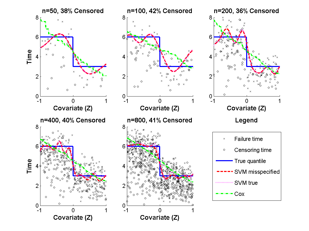
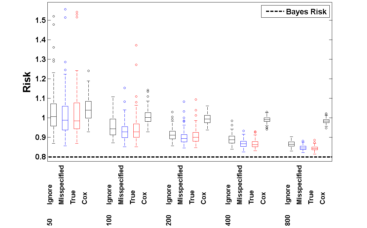
In the fifth setting, we consider a non-smooth conditional median. We also investigate the influence of using a misspecified model for the censoring mechanism. The covariates $Z$ are generated uniformly on the segment $[-1,1]$ . The failure time is normally distributed with expectation $3+3\bm{1}{\left\{Z<0\right\}}$ and variance $1$ . Note that the proportional hazards assumption does not hold for the failure time. The censoring variable $C$ follows the Weibull distribution with shape parameter $2$ , and scale parameter $-0.5Z+log(6)$ which results in mean censoring percentage of $40\%$ . Note that for this model, the censoring is independent of the failure time only given the covariate $Z$ (see Assumption (A2)). Estimation of the censoring distribution using the Kaplan-Meier corresponds to estimation under a misspecified model. Since the censoring follows the proportional hazards assumption, estimation using the Cox estimator corresponds to estimation under the true model. We use $5$ -fold-cross-validation to choose the regularization constant and the width of the kernel, as in setting 1.

In Figure 7, the conditional median obtained by the censored SVM learning method using both the misspecified and true model for the censoring, and by Cox regression, are plotted. The true median is plotted as a reference. In Figure 8, we compare the risk of the SVM method using both the misspecified and true model for the censoring. We also examined the effect of ignoring the censored observations. Both figures show that in general SVM does better than the Cox model, regardless of the censoring estimation. The difference between the misspecified and true model for the censoring is small and the corresponding curves in Figure 7 almost coincide. Figure 8 shows again that there is a non-negligible price for ignoring the censored observations.

7 Concluding Remarks

We studied an SVM framework for right censored data. We proposed a general censored SVM learning method and showed that it is well defined and measurable. We derived finite sample bounds on the deviation from the optimal risk. We proved risk consistency and computed learning rates. We discussed misspecification of the censoring model. Finally, we performed a simulation study to demonstrate the censored SVM method.

We believe that this work illustrates an important approach for applying support vector machines to right censored data, and to missing data in general. However, many open questions remain and many possible generalizations exist. First, we assumed that censoring is independent of failure time given the covariates, and the probability that no censoring occurs is positive given the covariates. It should be interesting to study the consequences of violation of one or both assumptions. Second, we have used the inverse-probability-of-censoring weighting to correct the bias induced by censoring. In general, this is not always the most efficient way of handling missing data (see, for example, van der Vaart, 2000, Chapter 25.5). It would be worthwhile to investigate whether more efficient methods could be developed. Third, we discussed only right-censored data and not general missing mechanisms. We believe that further development of SVM techniques that are able to better utilize the data and to perform under weaker assumptions and in more general settings is of great interest.

Appendix A Proofs

A.1 Auxiliary Results

The following result is due to 24 and is used to prove Theorem 17. Since it is not stated as a result there, we state the result and sketch the proof.

Theorem 30.

Let $L$ be a loss function and $H$ be an RKHS that satisfies assumptions (B1)–(B3). Let $f_{0}$ be such that $\|L(z,y,f_{0}(z))\|_{\infty}\leq B_{0}$ for some $B_{0}\geq B$ . Fix $\lambda>0$ and $\eta>0$ , and let $f\in H$ . Then for all $n\geq 72\eta$ , with probability not less than $1-e^{\eta}$ ,

		$\displaystyle(P-\mathbb{P}_{n})(L\circ\accentset{\frown}{f}-L\circ f_{P,L}^{*})<$
		$\displaystyle\qquad\frac{17}{27}\left(\lambda\\|f\\|^{2}_{H}+P(L\circ\accentset{\frown}{f}-L\circ f_{P,L}^{*})+\left(\frac{72V\eta}{n}\right)^{\frac{1}{2-\vartheta}}\right)+W\left(\frac{a^{2p}}{\lambda^{p}n}\right)^{\frac{1}{2-p-\vartheta+\vartheta p}}\,,$

where $W>1$ is a constant that depends only on $p$ , $M$ , $\vartheta$ , and $V$ , but not on $f$ .

Proof.

The proof is based on the proofs of Theorems 17.16, 17.20, and 17.23 of 24. We now present a sketch of the proof for completeness.

We first note that if $a^{2p}>\lambda^{p}n$ , it follows from (8) that the bound holds for $W\geq 4B$ . Thus, we consider the case in which $a^{2p}\leq\lambda^{p}n$ .

Let

\displaystyle r^{*}=\inf_{f\in H}\lambda\|f\|^{2}_{H}+\mathcal{R}_{L,P}(\accentset{\frown}{f})-\mathcal{R}_{L,P}^{*}\,.

For every $r>r^{*}$ , write

	$\displaystyle\mathcal{F}_{r}=$	$\displaystyle\left\{f\in H,\lambda\\|f\\|^{2}_{H}+\mathcal{R}_{L,P}(\accentset{\frown}{f})-\mathcal{R}_{L,P}^{*}\leq r\right\}\,,$
	$\displaystyle\mathcal{H}_{r}=$	$\displaystyle\left\{L\circ f-L\circ f_{P,L}^{*},f\in\mathcal{F}_{r}\right\}\,.$

Define

\displaystyle g_{f,r}=\frac{Ph_{\accentset{\frown}{f}}-h_{\accentset{\frown}{f}}}{\lambda\|f\|^{2}_{H}+\mathcal{R}_{L,P}(\accentset{\frown}{f})-\mathcal{R}_{L,P}^{*}}\,,\qquad f\in H,\;r>r^{*}\,.

Note that for every $f\in H$ , $\|g_{f,r}\|_{\infty}\leq 2Br^{-1}$ . It can be shown (24, Eq. 7.43 and the discussion there) that $Pg_{f,r}^{2}\leq Vr^{\vartheta-2}$ . Using Talagrand’s inequality (24, Theorem 7.5) we obtain

\displaystyle P\left(\sup_{f\in H}\mathbb{P}_{n}g_{f,r}\leq(1+\gamma)P[\sup_{f\in H}|\mathbb{P}g_{f,r}|]+\sqrt{\frac{2\eta Vr^{\vartheta-2}}{n}}+\left(\frac{2}{3}+\frac{1}{\gamma}\right)\frac{2\eta B}{nr}\right)\geq 1-e^{-\eta}

(18)

for every fixed $\gamma>0$ . Using Assumption (A3), it can be shown that there is a constant $\tilde{W}$ that depends only on $p$ , $M$ , $\vartheta$ , and $V$ , such that for every $r>\tilde{W}\left(\frac{a^{2p}}{\lambda^{p}n}\right)^{\frac{1}{2-p-\vartheta+\vartheta p}}$

\displaystyle P[\sup_{f\in H}|\mathbb{P}g_{f,r}|]\leq\frac{8}{30}

(19)

(see proofs of Theorems 7.20 and 7.23 of 24, for details). Substituting $\gamma=1/4$ in (18), and using the bound (19), we obtain that with probability of not less than $1-e^{\eta}$ ,

\displaystyle\sup_{f\in H}\mathbb{P}_{n}g_{f,r}\leq\frac{1}{3}+\sqrt{\frac{2\eta Vr^{\vartheta-2}}{n}}+\frac{28\eta B}{3nr}

(20)

for all $r>\tilde{W}\left(\frac{a^{2p}}{\lambda^{p}n}\right)^{\frac{1}{2-p-\vartheta+\vartheta p}}$ .

Using the fact that $n\geq 72\eta$ , some algebraic manipulations (see 24, proof of Theorem 7.23 for details) yield that for all $r\geq\left(\frac{72V\eta}{n}\right)^{1/(2-\vartheta)}$

\displaystyle\sqrt{\frac{2\eta Vr^{\vartheta-2}}{n}}\leq\frac{1}{6}\qquad\,,\qquad\frac{28\eta B}{3nr}\leq\frac{7}{54}\,.

(21)

Fix $f\in H$ . Using the definition of $g_{f,r}$ , together with the estimates in (21) for the probability bound (20), we obtain that for

\displaystyle r=\tilde{W}\left(\frac{a^{2p}}{\lambda^{p}n}\right)^{\frac{1}{2-p-\vartheta+\vartheta p}}+\left(\frac{72V\eta}{n}\right)^{1/(2-\vartheta)}

the inequality

\displaystyle(P-\mathbb{P}_{n})(L\circ\accentset{\frown}{f}-L\circ f_{P,L}^{*})<\frac{17}{27}\left(\lambda\|f\|^{2}_{H}+P(L\circ\accentset{\frown}{f}-L\circ f_{P,L}^{*})+r\right)

holds with probability not less than $1-e^{\eta}$ , and the desired result follows. ∎

A.2 Proof of Theorem 17

Proof of Theorem 17.

Note that by the definition of $f^{c}_{D,\lambda}$ ,

\displaystyle\lambda\|f^{c}_{D,\lambda}\|_{H}^{2}+\mathcal{R}_{L^{n}_{D},D}(\accentset{\frown}{f}^{c}_{D,\lambda})\leq\lambda\|f_{0}\|_{H}^{2}+\mathcal{R}_{L^{n}_{D},D}(f_{0}),

where $\mathcal{R}_{L^{n}_{D},D}(f)=\mathbb{P}_{n}\delta L(Z,Y(U),f(Z))/\hat{G}_{n}(U|Z)$ . Hence,

\displaystyle\begin{split}&\lambda\|f^{c}_{D,\lambda}\|_{H}^{2}+\mathcal{R}_{L,P}(\accentset{\frown}{f}^{c}_{D,\lambda})-\mathcal{R}_{L,P}^{*}\\ \leq&\lambda\|f_{0}\|_{H}^{2}+\mathcal{R}_{L^{n}_{D},D}(f_{0})-\mathcal{R}_{L^{n}_{D},D}(\accentset{\frown}{f}^{c}_{D,\lambda})+\mathcal{R}_{L,P}(\accentset{\frown}{f}^{c}_{D,\lambda})-\mathcal{R}_{L,P}^{*}\\ =&\left(\lambda\|f_{0}\|_{H}^{2}+\mathcal{R}_{L,P}(f_{0})-\mathcal{R}_{L,P}^{*}\right)+\left(\mathcal{R}_{L^{n}_{D},D}(f_{0})-\mathcal{R}_{L_{G},D}(f_{0})\right)\\ &\,+\left(\mathcal{R}_{L_{G},D}(f_{0})-\mathcal{R}_{L,P}(f_{0})+\mathcal{R}_{L,P}(\accentset{\frown}{f}^{c}_{D,\lambda})-\mathcal{R}_{L_{G},D}(\accentset{\frown}{f}^{c}_{D,\lambda})\right)+\left(\mathcal{R}_{L_{G},D}(\accentset{\frown}{f}^{c}_{D,\lambda})-\mathcal{R}_{L^{n}_{D},D}(\accentset{\frown}{f}^{c}_{D,\lambda})\right)\\ \equiv&A_{n}+B_{n}+C_{n}+D_{n}\,,\end{split}

(22)

where

\displaystyle\mathcal{R}_{L_{G},D}(f)\equiv\mathbb{P}_{n}L_{G}(Z,U,\delta,f(Z))\equiv\mathbb{P}_{n}\delta L(Z,Y(U),f(Z))/G(T|Z)\,,

i.e., $\mathcal{R}_{L_{G},D}$ is the empirical loss function with the true censoring distribution function.

Using conditional expectation, we obtain that for every $f\in H$ ,

\displaystyle\begin{split}\mathcal{R}_{L,P}(f)&\equiv P[L(Z,Y,f(Z))]=P\left[P\left[\left.\frac{\delta}{G(T|Z)}L(Z,Y,f(Z))\right|Z,T\right]\right]\\ &=P[L_{G}(Z,U,\delta,f(Z)]=\mathcal{R}_{L_{G},P}(f)\,.\end{split}

(23)

Therefore, we can rewrite the term $C_{n}$ as

\displaystyle\begin{split}C_{n}\equiv&\mathcal{R}_{L_{G},D}(f_{0})-\mathcal{R}_{L,P}(f_{0})+\mathcal{R}_{L,P}(\accentset{\frown}{f}^{c}_{D,\lambda})-\mathcal{R}_{L_{G},D}(\accentset{\frown}{f}^{c}_{D,\lambda})\\ =&\bigl(\mathcal{R}_{L_{G},D}(f_{0})-\mathcal{R}_{L_{G},D}(f_{P,L}^{*})\bigr)-\bigl(\mathcal{R}_{L_{G},P}(f_{0})-\mathcal{R}_{L_{G},P}(f_{P,L}^{*})\bigr)\\ &+\bigl(\mathcal{R}_{L_{G},P}(\accentset{\frown}{f}^{c}_{D,\lambda})-\mathcal{R}_{L_{G},P}(f_{P,L}^{*})\bigr)-\bigl(\mathcal{R}_{L_{G},D}(\accentset{\frown}{f}^{c}_{D,\lambda})-\mathcal{R}_{L_{G},D}(f_{P,L}^{*})\bigr)\,,\end{split}

(24)

where $f_{P,L}^{*}$ is the Bayes decision function.

For every function $f\in H$ , define the functions $h_{f}:\mathcal{Z}\times\mathcal{T}\mapsto\mathbb{R}$ as

\displaystyle h_{f}(z,t)=L_{G}(z,t,f(z))-L_{G}(z,t,f_{P,L}^{*}(z))\,,

for all $z,t\in\mathcal{Z}\times\mathcal{T}$ . Using this notation, we can rewrite (24) as

\displaystyle C_{n}\equiv(\mathbb{P}_{n}-P)h_{f_{0}}+(P-\mathbb{P}_{n})h_{\accentset{\frown}{f}^{c}_{D,\lambda}}\,.

(25)

In order to bound $(\mathbb{P}_{n}-P)h_{f_{0}}$ we follow the same arguments that lead to 24 Eq. 7.42, adapted to our setting. Write

\displaystyle(\mathbb{P}_{n}-P)h_{f_{0}}=(\mathbb{P}_{n}-P)(h_{f_{0}}-h_{\accentset{\frown}{f}_{0}})+(\mathbb{P}_{n}-P)h_{\accentset{\frown}{f}_{0}}.

Since $L_{G}(z,t,f_{0}(z))-L_{G}(z,t,\accentset{\frown}{f}_{0}(z))\geq 0$ , we obtain from the definition of $L_{G}$ , (8) and the bound on $f_{0}$ that $h_{f_{0}}-h_{\accentset{\frown}{f}_{0}}\in[0,B_{0}/2K]$ . It thus follows that

\displaystyle P\left((h_{f_{0}}-h_{\accentset{\frown}{f}_{0}})-P(h_{f_{0}}-h_{\accentset{\frown}{f}_{0}})\right)^{2}\leq P(h_{f_{0}}-h_{\accentset{\frown}{f}_{0}})^{2}\leq\frac{B_{0}}{2K}P(h_{f_{0}}-h_{\accentset{\frown}{f}_{0}})\,.

Using Bernstein’s inequality for the function $h_{f_{0}}-h_{\accentset{\frown}{f}_{0}}-P(h_{f_{0}}-h_{\accentset{\frown}{f}_{0}})$ , we obtain that with probability not less than $1-e^{-\eta}$ ,

\displaystyle(\mathbb{P}_{n}-P)(h_{f_{0}}-h_{\accentset{\frown}{f}_{0}})\leq\sqrt{\frac{\eta B_{0}P(h_{f_{0}}-h_{\accentset{\frown}{f}_{0}})}{Kn}}+\frac{B_{0}\eta}{3Kn}\,.

Using $\sqrt{ab}\leq\frac{a}{2}+\frac{b}{2}$ , we obtain

\displaystyle\sqrt{\frac{\eta B_{0}P(h_{f_{0}}-h_{\accentset{\frown}{f}_{0}})}{Kn}}\leq P(h_{f_{0}}-h_{\accentset{\frown}{f}_{0}})+\frac{B_{0}\eta}{4Kn}\,,

which leads to the bound

\displaystyle(\mathbb{P}_{n}-P)(h_{f_{0}}-h_{\accentset{\frown}{f}_{0}})\leq P(h_{f_{0}}-h_{\accentset{\frown}{f}_{0}})+\frac{7B_{0}\eta}{12Kn}\,,

(26)

which holds with probability not less than $1-e^{-\eta}$ .

Note that by the definition of $L_{G}$ , we have

\displaystyle\begin{split}Ph_{\accentset{\frown}{f}}^{2}&\equiv P\left(\frac{\delta}{G(T-)}(L(Z,Y,\accentset{\frown}{f}(Z))-L(Z,Y,f_{P,L}^{*}(Z)))\right)\\ &=P\left(L(Z,Y,\accentset{\frown}{f}(Z))-L(Z,Y,f_{P,L}^{*}(Z))\right)\\ &\leq VP\left(L(Z,Y,\accentset{\frown}{f}(Z))-L(Z,Y,f_{P,L}^{*}(Z))\right)^{\vartheta}=VPh_{\accentset{\frown}{f}}^{\vartheta},\end{split}

(27)

where we used (23) in the equalities and (9) in the inequality. Let $\tilde{V}=\max\{V,(B/(2K))^{2-\vartheta}\}$ . It follows from the proof of 24, Eq. 7.8, together with (27), that with probability not less than $1-e^{-\eta}$

\displaystyle(\mathbb{P}_{n}-P)h_{\accentset{\frown}{f}_{0}}\leq Ph_{\accentset{\frown}{f}_{0}}+\left(\frac{2\tilde{V}\eta}{n}\right)^{\frac{1}{2-\vartheta}}+\frac{2B\eta}{3Kn}\,.

(28)

Summarizing, we obtain from (26) and (28) that

\displaystyle(\mathbb{P}_{n}-P)h_{f_{0}}\leq Ph_{f_{0}}+\left(\frac{2\tilde{V}\eta}{n}\right)^{\frac{1}{2-\vartheta}}+\frac{2B\eta}{3Kn}+\frac{7B_{0}\eta}{12Kn}\,.

(29)

We are now ready to bound the second term in (25). By Theorem 30, with probability not less than $1-e^{\eta}$ , for all $n\geq 72\eta$ ,

\displaystyle(P-\mathbb{P}_{n})h_{\accentset{\frown}{f}^{c}_{D,\lambda}}

\displaystyle<\frac{17}{27}\left(\lambda\|f^{c}_{D,\lambda}\|^{2}_{H}+Ph_{\accentset{\frown}{f}^{c}_{D,\lambda}}+\left(\frac{72\tilde{V}\eta}{n}\right)^{\frac{1}{2-\vartheta}}\right)+W\left(\frac{a^{2p}}{\lambda^{p}n}\right)^{\frac{1}{2-p-\vartheta+\vartheta p}},

where $W>1$ is a constant that depends only on $p$ , $M$ , $\vartheta$ , and $\tilde{V}$ .

We would like to bound the expressions $B_{n}$ and $D_{n}$ of (22). Note that for any function $f$ , we have

\displaystyle\begin{split}|\mathcal{R}_{L_{G},D}(\accentset{\frown}{f})-\mathcal{R}_{L^{n}_{D},D}(\accentset{\frown}{f})|&\equiv\left|\mathbb{P}_{n}\frac{\delta L(Z,Y,\accentset{\frown}{f}(Z))}{G(T|Z)}-\mathbb{P}_{n}\frac{\delta L(Z,Y,\accentset{\frown}{f}(Z))}{\hat{G}_{n}(T|Z)}\right|\\ &=\left|\mathbb{P}_{n}\frac{\delta L(Z,Y,\accentset{\frown}{f}(Z))}{G(T|Z)\hat{G}_{n}(T|Z)}\left(\hat{G}_{n}(T|Z)-G(T|Z)\right)\right|\\ &\leq\frac{B}{2K^{2}}\mathbb{P}_{n}|(\hat{G}_{n}-G)(T|Z)|\,,\end{split}

(30)

where the last inequality follows from condition (A1) and (8).

Summarizing, we obtain that with probability not less than $1-3e^{-\eta}$

	$\displaystyle\lambda\\|f^{c}_{D,\lambda}\\|_{H}^{2}+$	$\displaystyle\mathcal{R}_{L,P}(\accentset{\frown}{f}^{c}_{D,\lambda})-\mathcal{R}_{L,P}^{*}$
	$\displaystyle\leq\;\;$	$\displaystyle\lambda\\|f_{0}\\|_{H}^{2}+Ph_{f_{0}}+\left(\frac{2\tilde{V}\eta}{n}\right)^{\frac{1}{2-\vartheta}}+\frac{2B\eta}{3Kn}+\frac{7B_{0}\eta}{12Kn}+\frac{B}{2K^{2}}\mathbb{P}_{n}\|(\hat{G}_{n}-G)(T\|Z)\|$
		$\displaystyle+\frac{17}{27}\left(\lambda\\|f^{c}_{D,\lambda}\\|^{2}_{H}+Ph_{\accentset{\frown}{f}^{c}_{D,\lambda}}+\left(\frac{72\tilde{V}\eta}{n}\right)^{\frac{1}{2-\vartheta}}\right)+W\left(\frac{a^{2p}}{\lambda^{p}n}\right)^{\frac{1}{2-p-\vartheta+\vartheta p}}\,.$

Note that by conditional expectation (23), $RLP(\accentset{\frown}{f}^{c}_{D,\lambda})-\mathcal{R}_{L,P}^{*}=Ph_{\accentset{\frown}{f}^{c}_{D,\lambda}}$ . Since $\tilde{V}>(B/2K)^{2-\vartheta}$ and $n\geq 72\eta$ ,

\displaystyle\frac{2B\eta}{3Kn}\leq\frac{4}{3}\cdot\frac{B}{2K}\cdot\frac{1}{72}\cdot\frac{72\eta}{n}\leq\frac{1}{54}\tilde{V}^{1/(2-\vartheta)}\left(\frac{72\eta}{n}\right)^{1/(2-\vartheta)}\,.

Hence, using the fact that $6\leq 36^{1/(2-\vartheta)}$ , and some algebraic transformations, we obtain

		$\displaystyle\lambda\\|f^{c}_{D,\lambda}\\|_{H}^{2}+\mathcal{R}_{L,P}(\accentset{\frown}{f}^{c}_{D,\lambda})-\mathcal{R}_{L,P}^{*}$
		$\displaystyle\leq\frac{27}{10}\left(\lambda\\|f_{0}\\|_{H}^{2}+Ph_{f_{0}}+\frac{36^{\frac{1}{2-\vartheta}}}{6}\left(\frac{2\tilde{V}\eta}{n}\right)^{\frac{1}{2-\vartheta}}+\frac{1}{54}\left(\frac{72\tilde{V}\eta}{n}\right)^{1/(2-\vartheta)}\right.$
		$\displaystyle\left.\quad+\frac{7B_{0}\eta}{12Kn}+2\cdot\frac{B}{2K^{2}}\mathbb{P}_{n}\|(\hat{G}_{n}-G)(T\|Z)\|+\frac{17}{27}\left(\frac{72\tilde{V}\eta}{n}\right)^{\frac{1}{2-\vartheta}}+W\left(\frac{a^{2p}}{\lambda^{p}n}\right)^{\frac{1}{2-p-\vartheta+\vartheta p}}\right)$
		$\displaystyle\leq\frac{27}{10}(\lambda\\|f_{0}\\|_{H}^{2}+Ph_{f_{0}})+\frac{27}{10}\frac{22}{27}\left(\frac{72\tilde{V}\eta}{n}\right)^{1/(2-\vartheta)}$
		$\displaystyle\quad+\frac{27}{10}\frac{7B_{0}\eta}{12Kn}+W\left(\frac{a^{2p}}{\lambda^{p}n}\right)^{\frac{1}{2-p-\vartheta+\vartheta p}}+\frac{27}{10}\frac{B}{K^{2}}\mathbb{P}_{n}\|(\hat{G}_{n}-G)(T\|Z)\|$
		$\displaystyle\leq 3(\lambda\\|f_{0}\\|_{H}^{2}+Ph_{f_{0}})+3\left(\frac{72\tilde{V}\eta}{n}\right)^{1/(2-\vartheta)}+\frac{8B_{0}\eta}{5Kn}+\frac{3B}{K^{2}}\mathbb{P}_{n}\|(\hat{G}_{n}-G)(T\|Z)\|+W\left(\frac{a^{2p}}{\lambda^{p}n}\right)^{\frac{1}{2-p-\vartheta+\vartheta p}}\,.$

Until now we assumed that $n\geq 72\eta$ . Assume now that $n<72\eta$ . By substituting the bounds (25), (29) and (30) in (22), we obtain the following bound, that holds with probability not less than $1-2e^{-\eta}$ , and where we did not use any assumption on the relation between $n$ and $\eta$ :

	$\displaystyle\lambda\\|f^{c}_{D,\lambda}\\|_{H}^{2}+\mathcal{R}_{L,P}(\accentset{\frown}{f}^{c}_{D,\lambda})-\mathcal{R}_{L,P}^{*}\leq$	$\displaystyle\left(\lambda\\|f_{0}\\|_{H}^{2}+\mathcal{R}_{L,P}(f_{0})-\mathcal{R}_{L,P}^{*}\right)+\frac{B}{K^{2}}\mathbb{P}_{n}\|(\hat{G}_{n}-G)(T\|Z)\|$
		$\displaystyle+\left(\frac{2\tilde{V}\eta}{n}\right)^{\frac{1}{2-\vartheta}}+\frac{2B\eta}{3Kn}+\frac{7B_{0}\eta}{12Kn}+(P-\mathbb{P}_{n})h_{\accentset{\frown}{f}^{c}_{D,\lambda}}\,.$

By the definition of $h_{\accentset{\frown}{f}^{c}_{D,\lambda}}$ , we obtain that $(P-\mathbb{P}_{n})h_{\accentset{\frown}{f}^{c}_{D,\lambda}}\leq B/K$ . Using the fact that $B/2K\leq\tilde{V}^{1/(2-\vartheta)}$ , we obtain that

\displaystyle(P-\mathbb{P}_{n})h_{\accentset{\frown}{f}^{c}_{D,\lambda}}\leq 2\left(\frac{72\tilde{V}\eta}{n}\right)^{1/(2-\vartheta)}

and thus the result follows also for the case $n<72\eta$ . ∎

A.3 Additional Proofs

Proof of Lemma 13.

Define

\displaystyle g(z,y)=\inf_{s}L(z,y,s)\,,\qquad\qquad(z,y,s)\in\mathcal{Z}\times\mathcal{Y}\times\mathbb{R}\,.

By assumption, for every $(z,y)\in\mathcal{Z}\times\mathcal{Y}$ , $\inf_{s}L(z,y,s)$ is obtained at some point $s=s(z,y)$ . Moreover, since $L$ is strictly convex, $s_{0}$ is uniquely defined.

We now show that $g(z,y)$ is continuous at a general point $(z_{0},y_{0})$ . Let $\{(z_{n},y_{n})\}$ be any sequence that converges to $(z_{0},y_{0})$ . Let $m_{n}=g(z_{n},y_{n})=L(z_{n},y_{n},s_{n})$ , and assume by contradiction that $m_{n}$ does not converge to $m_{0}=g(z_{0},y_{0})$ . Since $g(z,y)$ is bounded from above by $\max_{z,y}L(z,y,0)$ and $\mathcal{Z}\times\mathcal{Y}$ is compact, there is a subsequence $\{m_{n_{k}}\}$ that converges to some $m^{*}\neq m_{0}$ . By the continuity of $L$ , there is a further subsequence $\{s_{n_{k_{l}}}\}\in(-\infty,\infty)$ such that $L(z_{n_{k_{l}}},y_{n_{k_{l}}},s_{n_{k_{l}}})=m_{n_{k_{l}}}$ and $\{s_{n_{k_{l}}}\}$ converges to $s^{*}\in[-\infty,\infty]$ . If $s^{*}\in(-\infty,\infty)$ , then by definition $m_{0}=\inf_{s}L(z_{0},y_{0},s)<L(z_{0},y_{0},s^{*})=m^{*}$ , and hence from the continuity of $L$ for all $n$ large enough $L(z_{n_{k_{l}}},y_{n_{k_{l}}},s_{0})<L(z_{n_{k_{l}}},y_{n_{k_{l}}},s_{n_{k_{l}}})$ , and we arrive at a contradiction.

Assume now that $s^{*}\notin(-\infty,\infty)$ , and without loss of generality, let $s^{*}=\infty$ . Note that $\max_{z,y}g(z,y)$ is bounded from above by $M_{0}=\max_{z,y}L(z,y,0)$ . Chose $s_{M}>s_{0}$ such that for all $s>s_{M}$ , $L(z_{0},y_{0},s)>3M_{0}$ . By the continuity of $L$ , there is an $\varepsilon>0$ such that for all $(z,y)\in B_{\varepsilon}(z_{0},y_{0})\cap\mathcal{Z}\times\mathcal{Y}$ , $L(z,y,s_{M})>2M_{0}$ , and note that $L(z,y,s_{0})<2M_{0}$ . Recall that $L$ is strictly convex in the last variable, and hence it must be increasing at $s_{M}$ for all points $(z,y)\in B_{\varepsilon}(z_{0},y_{0})\cap\mathcal{Z}\times\mathcal{Y}$ (see for example Niculescu and Persson, 2006, Proposition 1.3.5). Consequently, for all $n$ big enough, $L(z_{n_{k_{l}}},y_{n_{k_{l}}},s_{n_{k_{l}}})>2M_{0}$ , and we again arrive at a contradiction, since $m_{n_{k_{l}}}<M_{0}$ .

We now show that $s(z,y)=\operatornamewithlimits{argmin}_{s}L(z,y,s)$ is continuous at a general point $(z_{0},y_{0})$ . Let $\{(z_{n},y_{n})\}$ be a sequence that converges to $(z_{0},y_{0})$ . Let $s_{n}=s(z_{n},y_{n})$ . Assume, by contradiction, that $s_{n}$ does not converge to $s_{0}$ . Hence, there is a subsequence $\{s_{n_{k}}\}$ that converges to some $s^{*}\in(-\infty,\infty)$ ( $s^{*}\in\{-\infty,\infty\}$ cannot happen, see above). Hence, $\lim L(z_{n_{k}},y_{n_{k}},s_{n_{k}})=\lim m_{n_{k}}=m_{0}$ , and $L(z_{0},y_{0},s_{0})=L(z_{0},y_{0},s^{*})=m_{0}$ , which contradicts the fact that $L(z_{0},y_{0},\cdot)$ is strictly convex and therefore has a unique minimizer.

Since $s(z,y)$ is continuous on a compact set, there is an $M$ such that $|s(z,y)|<M$ . It then follows from Lemma 2.23 of 24 that $L$ can be clipped at $M$ . ∎

{supplement}

[id=sec:suppA] \snameSupplement A \stitleMatlab Code \slink[url]http://stat.haifa.ac.il/ ygoldberg/research \sdescriptionPlease read the file README.pdf for details on the files in this folder.

References

Biganzoli et al. [1998] E. Biganzoli, P. Boracchi, L. Mariani, and E. Marubini. Feed forward neural networks for the analysis of censored survival data: A partial logistic regression approach. Statist. Med., 17(10):1169–1186, 1998.
Bitouzé et al. [1999] D. Bitouzé, B. Laurent, and P. Massart. A Dvoretzky-Kiefer-Wolfowitz type inequality for the Kaplan-Meier estimator. Ann. Inst. H. Poincaré Probab. Statist., 35(6):735–763, 1999.
Chen and Tsiatis [2001] P. Chen and A. A. Tsiatis. Causal inference on the difference of the restricted mean lifetime between two groups. Biometrics, 57(4):1030–1038, 2001.
Dabrowska [1987] D. M. Dabrowska. Non-Parametric regression with censored survival time data. Scandinavian Journal of Statistics, 14(3):181–197, 1987.
Dabrowska [1989] D. M. Dabrowska. Uniform consistency of the kernel conditional Kaplan-Meier estimate. The Annals of Statistics, 17(3):1157–1167, 1989.
Fleming and Harrington [1991] T. R. Fleming and D. P. Harrington. Counting processes and survival analysis. Wiley, 1991.
Goldberg and Kosorok [2012a] Y. Goldberg and M. R. Kosorok. An exponential bound for Cox regression. Statistics & Probability Letters, 82(7):1267–1272, 2012a.
Goldberg and Kosorok [2012b] Y. Goldberg and M. R. Kosorok. Q-learning with censored data. The Annals of Statistics, 40(1):529–560, 2012b.
Goldberg and Kosorok [2013] Y. Goldberg and M. R. Kosorok. Hoeffding-type and Bernstein-type inequalities for right censored data. Unpublished manuscript, 2013.
Gonzalez-Manteiga and Cadarso-Suarez [1994] W. Gonzalez-Manteiga and C. Cadarso-Suarez. Asymptotic properties of a generalized Kaplan-Meier estimator with some applications. Journal of Nonparametric Statistics, 4(1):65–78, 1994.
Guyon et al. [2002] I. Guyon, J. Weston, S. Barnhill, and V. Vapnik. Gene selection for cancer classification using support vector machines. Machine Learning, 46(1-3):389–422, 2002.
Hothorn et al. [2004] T. Hothorn, B. Lausen, A. Benner, and M. Radespiel-Tröger. Bagging survival trees. Statistics in medicine, 23(1):77–91, 2004.
Ishwaran and Kogalur [2010] H. Ishwaran and U. B. Kogalur. Consistency of random survival forests. Statistics & Probability Letters, 80(13-14):1056–1064, 2010.
Ishwaran et al. [2008] H. Ishwaran, U. B. Kogalur, E. H. Blackstone, and M. S. Lauer. Random survival forests. The Annals of Applied Statistics, 2(3):841–860, 2008.
Johnson et al. [2004] B. A. Johnson, D. Y. Lin, J. S. Marron, J. Ahn, J. Parker, and C. M. Perou. Threshhold analyses for inference in high dimension low sample size datasets with censored outcomes. Unpublished manuscript, 2004.
Karrison [1997] T. G. Karrison. Use of Irwin’s restricted mean as an index for comparing survival in different treatment groups–Interpretation and power considerations. Controlled Clinical Trials, 18(2):151–167, 1997.
Lawless [2003] J. F. Lawless. Statistical models and methods for lifetime data. Wiley, 2003.
Niculescu and Persson [2006] C. Niculescu and L. E. Persson. Convex Functions and their Applications. Springer, 2006.
Ripley and Ripley [2001] B. D. Ripley and R. M. Ripley. Neural networks as statistical methods in survival analysis. In Ri. Dybowski and V. Gant, editors, Clinical Applications of Artificial Neural Networks, pages 237–255. Cambridge University Press, 2001.
Robins et al. [1994] J. M. Robins, A. Rotnitzky, and L. P. Zhao. Estimation of regression coefficients when some regressors are not always observed. Journal of the American Statistical Association, 89(427):846–866, 1994.
Segal [1988] M. R. Segal. Regression Trees for Censored Data. Biometrics, 44(1), 1988.
Shim and Hwang [2009] J. Shim and C. Hwang. Support vector censored quantile regression under random censoring. Computational Statistics & Data Analysis, 53(4):912–919, 2009.
Shivaswamy et al. [2007] P. K. Shivaswamy, W. Chu, and M. Jansche. A support vector approach to censored targets. In Proceedings of the 7th IEEE International Conference on Data Mining (ICDM 2007), Omaha, Nebraska, USA, pages 655–660. IEEE Computer Society, 2007.
Steinwart and Chirstmann [2008] I. Steinwart and A. Chirstmann. Support Vector Machines. Springer, 2008.
Tsiatis [2006] A. A. Tsiatis. Semiparametric theory and missing data. Springer, 2006.
van der Vaart [2000] A. W. van der Vaart. Asymptotic Statistics. Cambridge University Press, 2000.
van der Vaart and Wellner [1996] A. W. van der Vaart and J. A. Wellner. Weak Convergence and Empirical Processes: With Applications to Statistics. Springer, 1996.
Wellner [2007] J. Wellner. On an exponential bound for the Kaplan�Meier estimator. Lifetime Data Analysis, 13(4):481–496, 2007.
Zhao et al. [2011] Y. Zhao, D. Zeng, M. A. Socinski, and M. R. Kosorok. Reinforcement learning strategies for clinical trials in nonsmall cell lung cancer. Biometrics, 67(4):1422–1433, 2011.
Zhu and Kosorok [2011] R. Zhu and M. R. Kosorok. Recursively Imputed Survival Trees. Journal of the American Statistical Association, 107(497):331–340, 2011.
Zucker [1998] D. M. Zucker. Restricted mean life with covariates: Modification and extension of a useful survival analysis method. Journal of the American Statistical Association, 93(442):702–709, 1998.

	$\displaystyle\lambda\\|f^{c}_{D,\lambda}\\|_{H}^{2}+$	$\displaystyle\mathcal{R}_{L,P}(\accentset{\frown}{f}^{c}_{D,\lambda})-\mathcal{R}_{L,P}^{*}$
	$\displaystyle\leq\;\;$	$\displaystyle\lambda\\|f_{0}\\|_{H}^{2}+Ph_{f_{0}}+\left(\frac{2\tilde{V}\eta}{n}\right)^{\frac{1}{2-\vartheta}}+\frac{2B\eta}{3Kn}+\frac{7B_{0}\eta}{12Kn}+\frac{B}{2K^{2}}\mathbb{P}_{n}\|(\hat{G}_{n}-G)(T\|Z)\|$
		$\displaystyle+\frac{17}{27}\left(\lambda\\|f^{c}_{D,\lambda}\\|^{2}_{H}+Ph_{\accentset{\frown}{f}^{c}_{D,\lambda}}+\left(\frac{72\tilde{V}\eta}{n}\right)^{\frac{1}{2-\vartheta}}\right)+W\left(\frac{a^{2p}}{\lambda^{p}n}\right)^{\frac{1}{2-p-\vartheta+\vartheta p}}\,.$

		$\displaystyle\lambda\\|f^{c}_{D,\lambda}\\|_{H}^{2}+\mathcal{R}_{L,P}(\accentset{\frown}{f}^{c}_{D,\lambda})-\mathcal{R}_{L,P}^{*}$
		$\displaystyle\leq\frac{27}{10}\left(\lambda\\|f_{0}\\|_{H}^{2}+Ph_{f_{0}}+\frac{36^{\frac{1}{2-\vartheta}}}{6}\left(\frac{2\tilde{V}\eta}{n}\right)^{\frac{1}{2-\vartheta}}+\frac{1}{54}\left(\frac{72\tilde{V}\eta}{n}\right)^{1/(2-\vartheta)}\right.$
		$\displaystyle\left.\quad+\frac{7B_{0}\eta}{12Kn}+2\cdot\frac{B}{2K^{2}}\mathbb{P}_{n}\|(\hat{G}_{n}-G)(T\|Z)\|+\frac{17}{27}\left(\frac{72\tilde{V}\eta}{n}\right)^{\frac{1}{2-\vartheta}}+W\left(\frac{a^{2p}}{\lambda^{p}n}\right)^{\frac{1}{2-p-\vartheta+\vartheta p}}\right)$
		$\displaystyle\leq\frac{27}{10}(\lambda\\|f_{0}\\|_{H}^{2}+Ph_{f_{0}})+\frac{27}{10}\frac{22}{27}\left(\frac{72\tilde{V}\eta}{n}\right)^{1/(2-\vartheta)}$
		$\displaystyle\quad+\frac{27}{10}\frac{7B_{0}\eta}{12Kn}+W\left(\frac{a^{2p}}{\lambda^{p}n}\right)^{\frac{1}{2-p-\vartheta+\vartheta p}}+\frac{27}{10}\frac{B}{K^{2}}\mathbb{P}_{n}\|(\hat{G}_{n}-G)(T\|Z)\|$
		$\displaystyle\leq 3(\lambda\\|f_{0}\\|_{H}^{2}+Ph_{f_{0}})+3\left(\frac{72\tilde{V}\eta}{n}\right)^{1/(2-\vartheta)}+\frac{8B_{0}\eta}{5Kn}+\frac{3B}{K^{2}}\mathbb{P}_{n}\|(\hat{G}_{n}-G)(T\|Z)\|+W\left(\frac{a^{2p}}{\lambda^{p}n}\right)^{\frac{1}{2-p-\vartheta+\vartheta p}}\,.$

Support Vector Regression for Right Censored DataT1

Abstract

Keywords:

keywords

keywords

1 Introduction

2 Preliminaries

2.1 Data Setup

Example 1.

Example 2.

Example 3.

Remark 4.

2.2 Loss Functions

Example 5.

Example 6.

Example 7.

2.3 Support Vector Machine (SVM) Learning Methods

Theorem 8.

3 SVM for Survival Data without Censoring

4 Censored SVM

Lemma 9.

Proof.

Lemma 10.

Proof.

Definition 11.

Lemma 12.

Proof.

5 Theoretical Results

5.1 Clipped Censored SVM Learning Method

Lemma 13.

5.2 Finite Sample Bounds

Remark 14.

Remark 15.

Remark 16.

Theorem 17.

Corollary 18.

5.3 𝒫\mathcal{P}-universal Consistency

Remark 19.

Remark 20.

Remark 21.

Theorem 22.

Proof.

5.4 Learning Rates

Definition 23.

Lemma 24.

Example 25.

Example 26.

Proof of Lemma 24.

5.5 Misspecified Censoring Model

Theorem 27.

Proof.

Example 28.

Example 29.

6 Simulation Study

7 Concluding Remarks

Appendix A Proofs

A.1 Auxiliary Results

Theorem 30.

Proof.

A.2 Proof of Theorem 17

Proof of Theorem 17.

A.3 Additional Proofs

Proof of Lemma 13.

References

Support Vector Regression for Right Censored Data^T1

5.3 $\mathcal{P}$ -universal Consistency