Theory of electron-phonon superconductivity: Does retardation really lead to a small Coulomb pseudopotential?
Abstract
The theory of electron-phonon superconductivity depends on retardation drastically reducing effects of the strong Coulomb repulsion. The standard theory only treats the lowest order diagram, which is an uncontrolled approximation. We study retardation in the Hubbard-Holstein model in a controlled way using perturbation theory and dynamical mean-field theory. We calculate analytically second order results for the pseudopotential and demonstrate the validity up to intermediate couplings by comparison with non-perturbative results. Retardation effects are still operative, but less efficient, leading to somewhat larger values of . Therefore, our theory can help to understand situations where the standard theory yields overestimates for .
pacs
74.20.-z,71.10.-w,63.20.KrThe theory of superconductivity based on the electron-phonon mechanism has been very successful in describing the properties of many materials [1, 2]. The electron-phonon coupling is treated in the Migdal Eliashberg (ME) theory [3], which relies on Migdal’s theorem [4]. This employs the fact that typical electron () and phonon () energy scales differ largely. Then perturbation theory greatly simplifies as vertex corrections are small. This is true even for large values of the electron-phonon coupling parameter as long as remains small [4, 5, 6].
A crucial issue is the effect of the Coulomb repulsion, typically much larger than the phonon-induced attraction. The electronic repulsion in the pairing channel can be projected to the phonon scale. It is then strongly reduced due to retardation effects and one finds [7, 8, 9, 10],
| (1) |
often termed the Morel-Anderson (MA) pseudopotential. Here, , where is a typical screened Coulomb interaction and is the density of states (DOS) at the Fermi energy. Since usually , one finds that and often also . Eq. (1) leads to estimates of the order . This agrees rather well to the fitting parameter obtained from tunnelling spectroscopy for many conventional superconductors [1].
Although ME theory has been very successful, the treatment of the Coulomb repulsion is by no means rigorous [11]. For the electron-phonon interaction, Migdal’s theorem justifies the neglect of vertex corrections. For the Coulomb interaction there is no similar justification, and Eq. (1) is based on an uncontrolled approximation. As long as it has not been demonstrated that indeed is small, conventional superconductivity has not been properly explained. The purpose of this paper is to analyse higher order corrections to the MA result. We show that retardation effects also reduce higher order contributions beyond Eq. (1), although less efficiently. For moderate we then find that indeed is rather small, although somewhat larger than in the standard theory.
There are cases reported in the literature, e.g., V or Nb3Ge [1], where the experimental values for in the literature of the order substantially larger than the traditional quotes, even though the ratio is not much different. These are not well explained by Eq. (1). Density functional theory (DFT) [12] finds good agreement with the tunnelling results for the pairing function, but to explain the experimental values for , in some cases quite large values of have to be used . A prominent example is elemental Li at ambient pressure [13, 14], where the coupling constant was estimated to be [13, 15]. With this implies 1K, while experimentally 0.4mK[16], which requires . The role of the Coulomb pseudo potential was also discussed in the case of the alkali-doped fullerides. Here, the MA theory leads to a large reduction of due to couplings to higher sub-bands [17], although this is unphysical [18, 17] and raises serious questions about higher order corrections for molecular solids. Actually, it was found that superconductivity in fullerides is due to a complicated interplay between the Coulomb interaction and Jahn-Teller phonons [19, 20].
The MA theory corresponds to treating the irreducible vertex to first order in . Berk and Schrieffer [21] included a specific class of higher order diagrams describing the coupling to ferromagnetic (FM) spin fluctuations, addressing almost FM metals, like Pd. They found that retardation is ineffective for the added diagrams and that superconductivity is strongly suppressed, which can help to explain the cases when FM spin fluctuations are important. For the model considered below, we extend the MA approach by adding the second order term. This does not include a large enhancement of the spin susceptibility and therefore we address the large class of systems which are not close to a FM instability. We use a projection approach and provide numerical calculations of without further approximation, as well as approximate analytical calculations. We find that retardation effects lead to a reduction of also in the second order calculation, but less efficiently. Then we add the electron-phonon interaction and calculate the superconducting gap numerically and approximately analytically. The results are well understood by the derived results for . To check the range of validity, our calculations are compared with non-perturbative dynamical mean-field theory (DMFT), which include all higher order corrections. DMFT fully treats retardation effects, which are crucial for the Coulomb pseudopotential. We show that results based on the perturbation theory agree well with DMFT calculations up to intermediate couplings .
In this work we deal with generic features of electron-phonon superconductivity and do not carry out calculations for a specific material. We employ the Hubbard-Holstein model, which possesses all necessary ingredients,
| (2) | |||||
creates an electron at site with spin , and a phonon with oscillator frequency , . The electrons interact locally with a screened Coulomb interaction , and couple to an optical phonon with coupling constant . For infinite dimensions this model is solved exactly by the DMFT.
First we deduce from an analysis of the pairing instability, in the limit , . We define the symmetric matrix [22],
| (3) |
where is the inverse temperature, is the irreducible vertex in the particle-particle channel and the pair propagator is , where and is the local lattice Green’s function. is singular at . We introduce the “low-energy part”
| (4) |
such that , and is the the block for . If is singular, is also singular. The “folding in” of larger frequencies describes how retardation effects reduce effects of the Coulomb repulsion on low frequency properties. We first consider the lowest order term of in , . We focus on the dependence on the half-band width and assume a constant DOS, . It is a rather good approximation to write , if and 0 otherwise. With , takes the form,
| (5) |
which is separable and can be inverted exactly. Replacing summations by integrals, we find then
| (6) |
Comparison of Eq. (5) and (6) leads to the Coulomb pseudopotential, , as given in in Eq. (1).
We next consider the second order term of in , which comes from a crossed diagram,
| (7) |
where the particle-hole bubble is given by
| (8) |
We can write , , where is independent of and approximated as
| (9) |
where , and are suitable values for the constant DOS.
Because of the form of , in Eq. (4) cannot be inverted analytically. Instead we use the inverse of based on , now only correct to first order in . However, since the off-diagonal terms of in Eq. (4) are of order , the final analytical result is correct to order . We make an ansatz for similar to Eq. (1),
| (10) |
Eq. (9) shows that the “folding in” of for large frequencies gives a small contribution to . This implies a reduced effective band width for the second order term, described by the factor in the logarithm. Identifying with the analytical result correct to order , is obtained. Eq. (10) is then also correct to order .
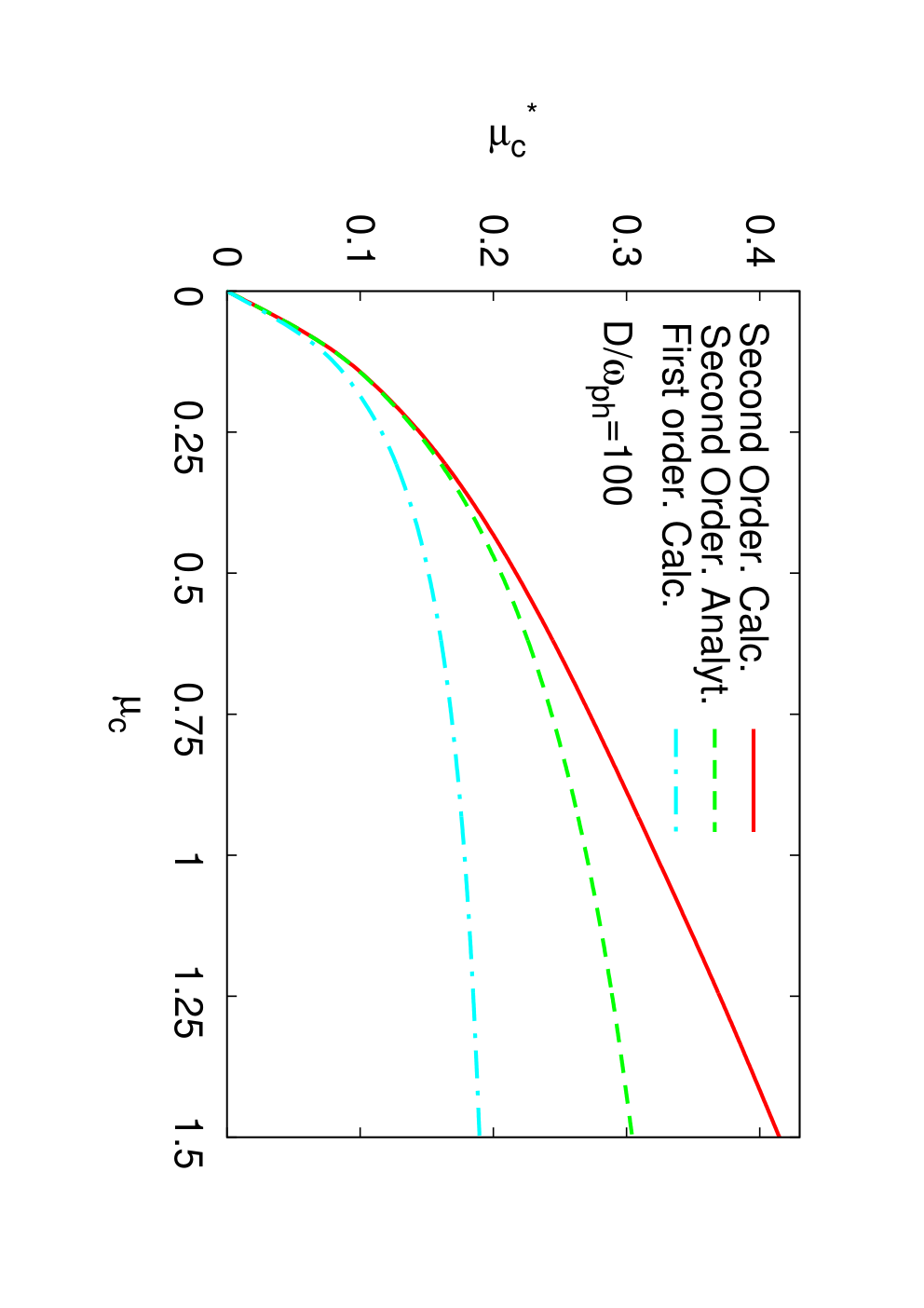
Fig. 1 shows results obtained by performing the calculations in Eq. (4) numerically using up to first or second order in and with . The analytical result in Eq. (10) are also shown. The second order result is clearly larger than the first order result. For , Eq. (10) describes the second order calculation rather well, while for larger corrections to the analytic result make still larger compared to Eq. (10). The second order contribution is reduced by retardation effects, but it is substantially less efficient than for the first order contribution, as described by the factor .
The MA theory [Eq. (1)] makes two main predictions: (i) as is increased for fixed and , goes to zero and (ii) as is increased for fixed , saturates at the value . (i) remains true when the second order contribution is taken into account, but the numerical result in Fig. 1 shows that (ii) is violated, i.e, does not saturate as is increased. Berk and Schrieffer [21] found that retardation is ineffective for higher order terms. They focused on almost FM metals for which the spin susceptibility is strongly enhanced for small and . This corresponds to low-lying excitations for which one expects small retardation effects. This is different from the situation considered here.
As a complimentary analysis, we extract results for from the spectral gap at . This is similar to the original work by Morel and Anderson [8], which included only the first order term in . We work on the imaginary axis in the limit . Starting point is the self-consistency equation for the off-diagonal self-energy,
| (11) |
where the kernel includes the attraction mediated by the phonons and the repulsion to order ,
| (12) |
is the offdiagonal Green’s function [23, 6] and a semi-elliptic DOS with is used. The effect of the diagonal self-energy is taken into account in the analytical calculations by a factor , which is taken finite only for [see Eq. (13)].
The self-consistency equation (11) can be solved numerically by iteration. For an analytical solution, we need to make some approximations. At half filling, we use for the Green’s function for ,
| (13) |
for , , and for , . A suitable ansatz for the off-diagonal self-energy is [8],
| (14) |
For we use Eq. (9), except that the numerical coefficients are modified for the semi-elliptic DOS. We have to solve for the three parameters , , and by evaluating the self-consistency equation at suitable values of . The general case is algebraically quite involved. Here, we only treat the first and purely second order cases explicitly to see the major effects.
For the first order case, we set and omit the -term in Eq. (12). We use the conditions , and . and assume . With the usual approximations we find a solution for the spectral gap of the form [24, 25],
| (15) |
The result for is given in Eq. (1) and .
In the situation when only the -term is included we set and omit the constant -term in Eq. (12). To determine the parameters and , we use the following two conditions: , and . The calculation again yields a result of the form (15), however, now with
| (16) |
As before accounts for the less effective retardation effects. In addition a term appears, which was absent in the first order calculation. Such terms can account for the discrepancy between analytical and numerical results in Fig. 1, where the analytical result saturates as function of . We obtain for .

In Fig. 2, we show the -dependence of the numerical solution of Eq. (11) for . It is compared with the analytical result in Eq. (15) with the respective results for , Eqs. (1,10,16). We use as before and . , were determined by fitting to the numerical solution for in the regime . was found to give a reasonable fit for the first order calculation in . We omit the term for the values of considered. The agreement between numerical and analytical results is quite good, which supports the earlier findings from the projection approach Eq. (4). One finds similar results as in Fig. 2 when calculating .

We now want to corroborate our findings with DMFT and analyse the impact of increasing on superconductivity similar to Fig. 2. For this purpose we need to include additional effects. We extended our previous DMFT and ME perturbation theory (PT) [6] to the case of finite . In the PT for and we include direct terms in up to second order, for instance, the terms described in Eq. (11). In addition, we have to take into account the fact that the electron-phonon vertex is renormalized by the Coulomb repulsion. We introduce the quantity , which contains and all corrections from the -term. For a weak frequency dependence up to the small phonon scale, we can define a renormalized coupling . For we use the result up to second order,
| (17) |
where and . This was found to give a good description up to [26]. Thus for the electron phonon part we use
| (18) |
where the phonon propagator is taken from the DMFT calculation [6]. The effective is defined by
| (19) |
where the phonon spectral function includes self-energy corrections due to . We define the renormalized phonon energy scale by the peak position of . Through the condition and a set of bare model parameters is determined by the DMFT calculations, for which we can compare the PT with DMFT. The results are shown in Fig. 3.
We find good agreement of the DMFT result with PT and the analytic formula, Eq. (15), up to . This demonstrates that (i) the electron-phonon vertex correction according to Eq. (17) is suitable, (ii) that the higher order form for the Coulomb pseudopotential in Eq. (10) captures correctly the results of the PT and the full DMFT calculation, and (iii) that the effective parameter description is appropriate. Therefore, this validates the previous analysis in a more complete calculation and it corroborates our findings for up to intermediate values of . For larger values of , we find that in the PT calculations exceeds the DMFT result, where . Then both Eq. (17) for and Eq. (10) for start to underestimate the reduction effect.
In conclusion, we emphasise that the standard theory of how retardation reduces is based on an uncontrolled approximation, since there is no Migdal’s theorem for the Coulomb interaction. In a controlled framework we analyse higher order corrections. We obtain an analytical expression for the next order term, and show that retardation also reduces this term, however substantially less efficiently. Non-perturbative DMFT calculations demonstrate that the perturbative result is accurate up to intermediate couplings. The main conclusion is then that retardation effects indeed lead to rather small values of , even when contributions beyond the standard theory are considered. For systems with sizable Coulomb interactions , our values for are larger than in the standard theory and lead to reduced values of the superconducting gap and . We have focused on the reduction of phonon induced s-wave superconductivity due to the Coulomb repulsion between electrons. Superconductivity which is induced in an anisotropic higher order angular momentum channel by purely repulsive interactions, such as the well-known Kohn-Luttinger effect [27], is not dealt with in the present work.
Acknowledgment -
We wish to thank N. Dupuis, A.C. Hewson, P. Horsch, C. Husemann, D. Manske, and R. Zeyher for helpful discussions. JH acknowledges support from the grant NSF DMR-0907150.
References
- [1] J. P. Carbotte, Rev. Mod. Phys. 62, 1027 (1990).
- [2] F. Marsiglio and J. Carbotte, in Superconductivity (Vol 1), edited by K. Bennemann and J. Ketterson (Springer, Berlin, 2008).
- [3] G. M. Eliashberg, Sov. Phys. JETP 11, 696 (1960).
- [4] A. B. Migdal, Sov. Phys. JETP 7, 996 (1958).
- [5] E. Maksimov and D. Khomskii, in High temperature Superconductivity, edited by V. Ginzburg and D. Kirzhnits (Consultants Publisher, New York, 1982).
- [6] J. Bauer, J. E. Han, and O. Gunnarsson, Phys. Rev. B 84, 184531 (2011).
- [7] N. Bogoliubov, V. Tolmachev, and D. Sirkov, in The Theory of Superconductivity, edited by N. Bogoliubov (Gordon and Breach, New York, 1962).
- [8] P. Morel and P. W. Anderson, Phys. Rev. 125, 1263 (1962).
- [9] J. R. Schrieffer, Theory of Superconductivity (W.A. Benjamin, Inc., New York, 1964).
- [10] D. J. Scalapino, in Superconductivity, edited by R. Parks (Marcel Dekker, New York, 1969).
- [11] P. B. Allen and B. Mitrovic, in Solid State Physics (Vol 37), edited by H. Ehrenreich, F. Seitz, and D. Turnbull (Academic, New York, 1982).
- [12] S. Y. Savrasov and D. Y. Savrasov, Phys. Rev. B 54, 16487 (1996).
- [13] A. Y. Liu and M. L. Cohen, Phys. Rev. B 44, 9678 (1991).
- [14] C. F. Richardson and N. W. Ashcroft, Phys. Rev. B 55, 15130 (1997).
- [15] T. Bazhirov, J. Noffsinger, and M. L. Cohen, Phys. Rev. B 84, 125122 (2011).
- [16] J. Tuoriniemi, K. Juntunen-Nurmilaukas, J. Uusvuori, E. Pentti, and A. Sebedash, Nature 447, 187 (2007).
- [17] O. Gunnarsson and G. Zwicknagl, Phys. Rev. Lett. 69, 957 (1992).
- [18] P. Anderson (1991), unpublished.
- [19] M. Capone, M. Fabrizio, C. Castellani, and E. Tosatti, Science 296, 2364 (2002).
- [20] J. E. Han, O. Gunnarsson, and V. H. Crespi, Phys. Rev. Lett. 90, 167006 (2003).
- [21] N. F. Berk and J. R. Schrieffer, Phys. Rev. Lett. 17, 433 (1966).
- [22] A. Georges, G. Kotliar, W. Krauth, and M. Rozenberg, Rev. Mod. Phys. 68, 13 (1996).
- [23] J. Bauer, A. C. Hewson, and N. Dupuis, Phys. Rev. B 79, 214518 (2009).
- [24] W. L. McMillan, Phys. Rev. 167, 331 (1968).
- [25] P. B. Allen and R. C. Dynes, Phys. Rev. B 12, 905 (1975).
- [26] Z. B. Huang, W. Hanke, E. Arrigoni, and D. J. Scalapino, Phys. Rev. B 68, 220507 (2003).
- [27] W. Kohn and J. M. Luttinger, Phys. Rev. Lett. 15, 524 (1965).