Constrained quantum mechanics: chaos in non-planar billiards
Abstract
We illustrate some of the techniques to identify chaos signatures at the quantum level using as a guiding examples some systems where a particle is constrained to move on a radial symmetric, but non planar, surface. In particular, two systems are studied: the case of a cone with an arbitrary contour or dunce hat billiard and the rectangular billiard with an inner Gaussian surface.
Keywords: quantum chaos, billiards, random matrices.
1 Introduction
Hard wall billiards are among the simplest and most studied systems in the field of classical and quantum chaos [1]-[5]. A two dimensional quantum billiard is analogous to a vibrating membrane because of the mathematical equivalence of the stationary Schrödinger and Helmholtz equation with the same Dirichlet boundary conditions. This similarity between billiards and classical waves has been used in experiments e.g. the quantum microwave cavities [6]. When the classical counterpart of these systems are chaotic, some signatures of this chaos appear at the quantum level. One of them is the statistical properties of the spectrum, which follow the Bohigas, Giannoni and Schmit conjecture [7]. This conjecture states that the nearest neighbour energy level statistics of a time reversal invariant chaotic system follows the same statistical as the ensemble of random orthogonal matrices with Gaussian distributed elements, i.e. the Gaussian Orthogonal Ensemble (GOE) [8]. For matrices this distribution, also known as the Wigner distribution, is given by
| (1) |
To be more precise, the energy levels should be first classified according to the partial symmetries that the system has, then the statistical analysis should performed on each symmetry class of states, and for each of those the nearest neighbour spacing distribution of the energy level, properly normalized, follows the GOE distribution (1). On the other hand, for systems with enough symmetries to be integrable, the nearest neighbour energy level statistics follows a Poisson distribution.
Additionally, quantum chaotic billiards exhibit the phenomenon of scarring of their wavefunction specially when the corresponding state is deep in the semiclassical limit [9]. Although, the scars in the wavefunction were first observed in the seventies [10] they have become a phenomenon of great interest because they represent a connection between the quantum chaotic billiard with its periodic orbits.
The chaotic features of two dimensional billiards are often studied confining them on a plane with a contour where chaos emerges when an “irregular” contour is used. However, the system present interesting features if we set a non-planar geometry in the billiard internal region , even when the contour is regular as a circle, a rectangle or an ellipse.
The aim of this work is to illustrate some of the characteristic signatures of chaos at the quantum level in non-planar billiards. As such, this paper is an introduction for graduate and advanced undergraduate students to the topic of chaos in quantum systems, illustrated in systems different than the usual planar billiards. It can serve as a guiding example to the techniques used to analyze and identify chaos signatures in quantum systems. Two systems are studied: the dunce hat billiard (or conical billiard) and the rectangular billiard with a Gaussian surface. These billiards are shown in figure 1.

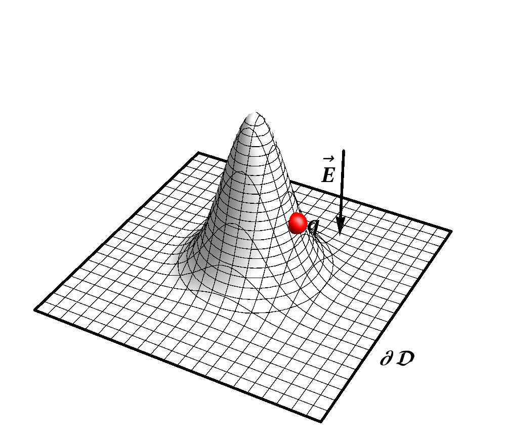
We start in section 2 with a geometrical background needed to study non-planar systems. Although most of this work is about quantum systems, in section 3, we study the classical dynamics on these billiards and present some of the chaos characteristic signatures at the classical level. Then we proceed, in section 4, to present how the quantum Hamiltonian is constructed on non-planar surfaces, and in sections 5 and 6 both types of billiards are studied at the quantum level.
2 Geometrical background
Consider a surface embedded in the three-dimensional Euclidean space defined by
| (2) |
where are the Cartesian coordinates in and are the Gaussian curvilinear coordinates defined on the surface. A particle restricted to move on a two-dimensional surface has only two degrees of freedom, and its position may be expressed as follows
| (3) |
The motion of a particle will depend of the surface geometry which is specified by the first and second fundamental forms. Several of the intrinsic properties of are determined by its metric included in the first fundamental form given by
| (4) |
We are interested in billiards with a radial symmetric surface defined by
| (5) |
For this particular case the metric is a diagonal tensor
| (6) |
Therefore, the system is orthogonal and the Gaussian curvature may be computed with
| (7) |
where . Replacing the metric given by the equation (6) we find
| (8) |
Classically, the motion of a particle which lives on is affected by the surface curvature because the surface metric is included explicitly in the kinetic energy, which is proportional to . At the quantum level, this kinetic energy is associated with the Laplace-Beltrami operator on the surface. Other extrinsic properties of are specified in its second fundamental form given by
| (9) |
and the matrix for a radial symmetric surface is
| (10) |
This enables to compute the principal curvatures and . If the principal directions coincide with coordinate curves, then
| (11) |
Finally, if the surface is radially symmetric, then
| (12) |
3 Classical motion
The Lagrangian in cylindrical coordinates of a particle of mass with a time independent potential is
| (13) |
The position of particle constrained to move on a radial symmetric surface defined by is . Then, the Lagrangian takes the form
| (14) |
with
| (15) |
so the canonical momentum is
| (16) |
Therefore, the Hamiltonian is
| (17) |
If the particle has a charge , and the system is placed in a uniform electric field (with ), then . Finally, the Hamiltonian is
| (18) |
and the Hamilton equations of motion for the -coordinate are
| (19) | |||||
| (20) |
The -component of the angular momentum remains constant in between two successive collisions of the particle with the billiard walls. As a result, for the -coordinate
| (21) |
where the billiard contour is and is a constant. The value of depends of the billiard contour. For instance, has the same value for all the collisions in a circular contour but in general it must be updated after each collision when the contour is not a circular one.
3.1 The dunce hat billiard map
After the plane surface, one of the simplest case of study with zero Gaussian curvature is the cone. Let us define the dunce hat billiard as a cone with a circular contour . The Hamiltonian of this billiard in absence of the electric field according the equation (18) is
| (22) |
This Hamiltonian differs from the free particle on the plane surface Hamiltonian for the constant term , and avoiding the circular contour the free particle solution on the cone is found by direct integration of the equations of motion. The position is given by
| (23) |
and
| (24) | |||||
where is the initial position of the particle in polar coordinates. The radial and angular velocity at are and respectively. Although, the structure of and on the cone is similar to the one obtained for the free particle on the plane surface, the cone may deflect the particle trajectory as it is shown in Figure 2.
The solution of the equations of motion on the cone, including the circular contour, may be found defining the following variable rescaling
| (25) |
The Lagrangian with the new variables takes the form
| (26) |
with and . The new canonical momenta are:
| (27) |
By computing the Poisson brackets of the new coordinates it can be checked that the transformation is canonical.


The region remains as a disk: . However, the contour is . The upper limit of may be written as where . If we take a circle of radius , then we may build a cone of radius and height by removing a circular section with angle . As a result, is just the angle related with the circular section removed from the circle in order to construct the cone. In the -plane we have a circular planar billiard. Therefore, if locates the n-collision and is the angle of the incident velocity of the n-collision, then the next collision is connected with the billiard map . This map for a circular billiard is given by [11]
| (28) |
with . Using the equation (28) the particle position is
| (29) |
| (30) |
Where is the time between successive collisions, and is the integer part of . According to the circular billiard map . Therefore, at the -th collision the particle is located at
| (31) |
The last expression gives us the position of each collision. However, this map does not specify how successive collisions are connected. As we show in Figure 2 the cone deflects the particle. Therefore, two successive collisions predicted by (31) must be connected by a curve (see Figure 3). This is an expected difference with the plane billiards where collisions are connected by rectilinear trajectories.
3.2 Classical rectangular billiard with an inner Gaussian surface
This billiard is a rectangular box with an inner Gaussian surface defined as where is the standard deviation and is a constant which we will set equal to one.
The classical trajectories become irregular as the Gaussian surface emerges in the interior of the rectangular billiard (Figure 4). The trajectories were found solving the equations of motion using the fourth order Runge-Kutta method between successive collisions. When the particle collided with the frontier, then its new momentum was found and the new trajectory before the next collision was computed numerically.
3.3 The phase space
The billiards described in this document have two degrees of freedom because the particle moves on a two-dimensional surface. Therefore, the phase space is four-dimensional. Taking into account that system is Hamiltonian then the motion takes place on a three dimensional hypersurface of the phase space and we need only three variables in order to describe it.


The Poincaré section is commonly used in order to map the system and to obtain its dynamical information. This is equivalent to consider two variables which define where and how the collision occurs. These variables are the collision location and the angle between the incident vector velocity projected in the plane with the normal vector of . The two variables of the mapping then define a reduced phase space. In the dunce hat billiard with circular contour the trajectories are periodic orbits if is a rational multiple of . These type of trajectories are presented in the reduced phase space by a set of points located in a horizontal line = constant where is the closed orbit period. On the other hand, if is a non-rational multiple of , the billiard will have a quasi periodic orbit. This trajectory is tangent to an inner circle in the surface and it fills it generating a caustic. A quasi-periodic orbit is represented as a straight horizontal and densely filled line in the reduced phase space. The phase space of the dunce hat billiard with rectangular contour and the rectangular billiard with Gaussian surface were built for a sample of trajectories starting from different random initial conditions (see Figure 5). When or , both billiards become the rectangular planar billiard. The phase space of this billiard has straight horizontal lines typical of a non chaotic billiard. On the other hand, the phase space is filled by a chaotic sea when a cone or a Gaussian surface emerge in the rectangular billiard.
4 Quantum Hamiltonian
At the quantum level, the Hamiltonian of the non-planar billiards considered here has the form
| (32) |
The terms involved in the Hamiltonian are:
(i) The kinetic energy on the surface. The Laplace-Beltrami operator is
| (33) |
with . Then, the kinetic energy may written as
| (34) |
where is the free particle Hamiltonian on the plane, and is a function with dimensions of wave vector defined by
| (35) |
Using the equation (8) the radial kinetic energy on the surface may be also expressed in terms of the normal Gaussian curvature as . Therefore, this term is null for some radially symmetric surfaces e.g. the plane and the cone. Finally, the non-dimensional function is defined by .
(ii) The surface confining potential. The constrain of classical mechanics which ties the particle to the surface, in quantum mechanics may be introduced by a confining potential which enforces the particle to stay on the surface. This known as the confining approach, and it predicts the following contribution to the quantum Hamiltonian [12, 13]
| (36) |
where and are the principal curvatures of the surface. For a radial symmetric two dimensional surface the principal directions are along and , then (see equation (12))
| (37) |
and
| (38) |
(ii) The external potential. This term includes the potential of the external electric field , and the corresponding potential due to the boundary of the billiard
| (39) |
where
| (40) |
and defines the contour of the billiard.
5 The quantum dunce hat billiard
5.1 The quantum dunce hat billiard with a circular contour
This is probably the simplest case of study. The Gaussian curvature , given by (8), is zero for this billiard as happens with the typical billiards in the plane. This makes a significant simplification in the Hamiltonian
| (41) |
where the confining potential is
| (42) |
We may expect that the effect of the confining potential should not be relevant because it may be absorbed in at least with a circular contour where commutes with the Hamiltonian by virtue of the radial symmetry of the billiard11 1 This will not be the case for an square contour where only some discrete symmetries of the billiard may remain depending the position of the cone center in the box.. The analytic solution for this system may be found using the transformation defined by the equation (25). After the change of variable the Hamiltonian takes the form
| (43) |
where , and . The eigenvectors and eigenvalues may be obtained by separation of variables. Substituting in the eigenvalue equation , one finds
| (44) |
The angular function is and it must fulfill with the condition , therefore . As result, the angular solution is the same obtained in the planar circular billiard
| (45) |
The radial part of the equation will lead as usual to the Bessel differential equation, but with a non integer index ,
| (46) |
Defining
| (47) |
the radial solution is
| (48) |
where () are the zeros of the Bessel function of the first kind . The corresponding energy levels are
| (49) |
Some eigenstates are shown in Figure 6 with a comparison with some classical trajectories.


Let us consider the energy staircase function . This function counts the number of states below the energy and it is defined by
| (50) |
where is the step function. Knowing the asymptotic behaviour of the large zeros of the Bessel function, one can obtain the asymptotic behaviour of for large , following similar steps as in the planar circular billiard [14]. At the first order, we find that
| (51) |
where is the area of the cone without including its base. The equation (51) is in agreement with the well known Weyl’s formula usually employed for quantum billiards in the plane
| (52) |
where and are the area and perimeter of the billiard. The confining potential constitutes a remarkable difference between quantum non-planar billiards and the quantum billiards in the plane. In fact, the confining potential changes the spectrum and the states. Nevertheless, the agreement between the Weyl’s formula and staircase function of the dunce hat billiard suggests that confining potential does not change the at least at the first order in the asymptotic limit.
Figure (7)-(left) shows how the energy levels are somehow “compressed” when the parameter is increased. Consequently, the number of energy levels below of a fixed energy must increase with . This is in agreement with (51).
The dunce hat billiard with a circular contour at the classical level is an integrable system. Hence, we expect that nearest neighbour energy level statistics will be a Poissonian in agreement with the Bohigas-Giannoni-Schmit conjecture [7]. This can be verified in Figure 7-(right).
5.2 The quantum dunce hat billiard with a rectangular contour
By changing the circular contour of the dunce hat billiard with rectangular one, the rotational symmetry of the system is broken, and the angular momentum is not conserved anymore. The system is no longer integrable. A radial symmetric deflector as the cone in combination with a square boundary induce complicated classical dynamics. Therefore, at the quantum level, the spectrum and eigenvectors are not simple in comparison with the ones obtained in the circular boundary case. We expect that the quantum dunce hat billiard in the square box will share some of the statistical properties in its spectrum with other quantum billiards with a classical chaotic counterpart.


In general, this billiard require a numerical treatment. We implemented the Finite Difference Method in order to solve the eigenproblem for the Hamiltonian. Some of the eigenstates are shown in Figure 8 and the nearest neighbour spacing distribution of the energy levels is shown in Figure 9. The cone has not been placed at the center of the box in order to break the remaining discrete symmetries and to avoid the symmetry classification of energy levels in the level statistics computation.
We have demonstrated that the staircase function of the dunce hat billiard with a circular box satisfies the Weyl’s formula (see equation (51)). As a result, we may expect that should be linear with for this billiard with an arbitrary contour, for large . We evidence this behaviour in the numerical computation of (see Figure 9-(left)) at least for . After this value the numerical staircase function was not linear because of the numerical error so we only use the first states in the level statistics computation.
The histogram of the nearest neighbour spacing distribution for the energy levels below the state 2000 is shown in Figure 9-(right). It fits the Gaussian Orthogonal Ensemble (GOE) distribution (1). Therefore, the change of the inner geometry of the two-dimensional square well from the plane to a cone produces the emerging of classical chaos as well as a change in the distribution of the energy levels of the billiard quantum counterpart.
6 Quantum billiard with a Gaussian surface
We may use the finite difference method in order to solve the problem for any surface with an arbitrary contour. For that purpose, the Hamiltonian given by the equation (32) is expressed as a matrix on a lattice and then it is diagonalized. However, in this section, an alternative way to solve numerically the non-integrable problem will be presented. The idea is to use the analytic eigenvectors of the planar billiard rectangular as a basis to expand the wavefunctions of the non-planar rectangular billiard. As an illustration, we will study the quantum rectangular billiard with a Gaussian surface.
6.1 Billiard with a rectangular contour
The eigenvectors of the rectangular plane billiard will be used as a basis to expand the eigenfunctions of the Hamiltonian (32), where
| (53) |
is the area of the box, and
| (54) |
The first kinetic term of the Hamiltonian expressed in is
where
| (56) |
are the eigenvalues of the plane billiard. In (), we have used the expansion
| (57) |
which requires , i.e., for the convergence of the geometric series.
Defining and using the binomial formula for in (), we obtain
| (58) | |||||
where
The super index means that the integrand has the product , and upper integration limit is with and . All the other terms in the Hamiltonian may be expressed in a similar way. After a lengthly, but simple algebra, we find
Confining potential terms
| (59) | |||||
and
| (60) |
where the functions must be evaluated at , and
| (61) |
Radial kinetic term
| (62) |
with
| (63) |
and
| (64) |
where
| (65) |
Centrifugal term
| (66) | |||||
where the functions must be evaluated at .
Electric potential term
| (67) |
where the functions must be evaluated at .
The functions and can be computed by successive differentiations with respect to of the corresponding function with , which can be computed numerically. Using the matrix elements previously computed, the Hamiltonian is diagonalized numerically.

The numerical results for the rectangular billiard with the Gaussian surface are shown in Figure 10. We have computed 5050 energy levels and the first 3500 of them were used to compute the nearest neighbour spacing distribution. The Gaussian surface is located in one of the rectangle corners. We have used a rectangle instead of a square in order to avoid the energy level classification by each symmetry. As in the case of a cone, the Gaussian surface introduces chaos in the classical motion which is translated at the quantum scale as a change of level statistics from a Poisson to a GOE distribution. Although, the histogram does not fit with the GOE distribution it does with the distribution function for mixture of chaos and regularity given by [15]
| (68) |
with . The function is a Poisson distribution for and it characterizes the regular behaviour of the classical counterpart. On the other hand, the function is a GOE distribution (1) for when the classical counterpart is fully chaotic. In general the Weyl’s formula does not apply for this billiard because the confining potential may change the spectral staircase function. However, the effect of this potential is negligible for high energy levels. This may be appreciated at the region where the numerical spectral staircase function has a linear behaviour (see Figure 10-(c)).
6.2 Quantum billiard immersed in a strong electric field
If the applied electric field is strong, then it would be unlikely to find the particle near the top of the Gaussian surface, at least for small values of the kinetic energy. On the other hand, the function affects the particle motion around the top of the surface where the slope of the Gaussian function is not zero. Therefore, in this limit the contribution of the centrifugal term is negligible because the particle hardly reach the region where is important. The situation is similar for the term, so under the condition of large the kinetic energy will be exclusively in . Then, the Hamiltonian takes the form
| (69) |
The eigenvalues and eigenvectors can be found numerically either by using the finite difference method, or the method explained in the previous section.


Two billiards will now be studied: the rectangular billiard with the Gaussian surface and its counterpart with a circular contour, both under the influence of a strong external electric field. These rectangular and circular billiards are analogous to the Sinai and annular billiard with a soft inner disk respectively.
For the circular billiard, if the center of the Gaussian surface is located at the center of the circular boundary, the system has a continuous rotational symmetry and the angular momentum is conserved. This two-dimensional system, having two constants of motion ( and ) is then integrable. The nearest neighbour spacing distribution of the energy levels is a Poisson distribution, a situation similar to the one shown in Figure 7-(right) for the dunce hat billiard with circular contour. If the rotational symmetry is broken by not placing the center of the Gaussian on the center of the circular boundary, then the system will be chaotic.


The symmetry group of the rectangular billiard with the Gaussian surface is the dihedral group . This is the same symmetry group of the Sinai billiard. Therefore, the rectangular billiard level statistics requires the energy levels classification by each billiard symmetry. We may avoid this symmetry classification by placing the Gaussian function away from the square center in order to break the billiard symmetries. If a symmetry axe is hold as we show in Figure 11-b and Figure 12-b (this also applies for the circular billiard), then the energy levels are divided into two sets according to the parity of the wavefunction. The nearest neighbour spacing distribution of the whole spectrum is the superposition of two independent GOE distributions, known as the GOE2 distribution
| (70) |
The histograms, for both the circular and rectangular billiard in this situation, are shown in Figures 11-d and 12-c.
On the other hand, if we break all the geometrical symmetries then the nearest neighbour spacing distribution of the rectangular billiard with strong field is a GOE distribution (1). This is a feature of classically chaotic systems with time reversal symmetry where the energy levels are likely to repel to each other (see Figure 11-e).
When one symmetry axe is kept, the GOE distribution can also be obtained by taking the energy levels of the odd or even states separately in the level statistics computation. Nevertheless, this process requires the computation of more energy levels because the parity classification enable us to use only approximately a half of the numerically admissible energy levels computed for each nearest neighbour spacing distribution.


Scars and bouncing ball states are another interesting phenomena observed in the standard quantum billiards. They are a manifestation of the classical features on the wavefunction of states in the semiclassical limit. The scarring of the wavefunction is a common characteristic of quantum billiards with classical chaotic counterpart. For the rectangular billiard with the Gaussian surface in a strong electric field, a wave function presenting scars is shown in Figure 13-(d). This state corresponds to the closed unstable orbit presented in Figure 13-(a). It is not a surprise to find scars in the rectangular and circular billiards with the Gaussian surface because of their similarity with the Sinai billiard and the annular billiard which also exhibit scars. However, here the scarring of the wavefunction of these billiards is a consequence of the external field and the modification of the billiard interior geometry. Taking into account that scarring does not appear in quantum billiards with regular classic analogue, then this phenomenon is another signature of chaos of the rectangular and circular billiards with a Gaussian surface with strong field at the quantum scale.
Another evidence of the classical aspects on the wavefunction are the bouncing ball states (see Figure 13 and Figure 14). These states differ from the scars because they represent a set of classical stable trajectories on the wavefunction. Thus a bouncing ball state represents a particle which has a well defined momentum but not a well defined position.


7 Concluding remarks
The classical chaotic behaviour of a particle in a two dimensional plane billiard depends of the billiard contour. However, the inner geometry of the billiard is also a determinant factor. We show that if we set a non planar surface into a billiard, then it may produce classical chaos which may be identified at the quantum scale, even with a regular contour (rectangular or circular). Some examples were studied in this paper namely: the dunce hat billiard and the billiard with a Gaussian surface with a rectangular or circular contours. We found that the Bohigas-Giannoni-Schmit conjecture remained valid for each of these billiards. Additionally, the billiards exhibited scarring of the wavefunction.
For the circular billiard, if the center of the surface (cone or Gaussian) is placed at the center of the boundary, the system is integrable because it has two constant of motion, the Hamiltonian and the -component of the angular momentum. We explicitly found analytically the spectrum and eigenvectors of the quantum dunce hat billiard with a circular contour. The effect of the surface was the rescaling of the spectrum by a global factor with respect to the one of a circular planar billiard. As a result, the nearest neighbour spacing distribution is the Poisson distribution.
To confine the particle to a non-planar surface, a confining potential should be added at the quantum level. This confining potential affects the billiard energy levels. However, if the particle energy is high, then the contribution of the confining potential term may be dropped. As a result, although the Weyl’s formula does not consider the quantum confining potential, it may be used in the asymptotic limit. This fact was analytically demonstrated with the quantum circular dunce hat billiard and numerically observed in the dunce hat and Gaussian billiards with a rectangular contour.
The finite difference method and the expansion method were implemented in order to diagonalize the Hamiltonian of the quantum rectangular billiard with the Gaussian surface. The advantage of the second method is that a comparison of the numerical staircase function of both methods showed that the second one required the truncation of a Hamiltonian to a smaller dimension in order to obtain a more energy levels with an acceptable numerical error. For this aim, we use the fact that the slope of the spectral staircase function is just for a large energy where the confining potential may be neglected.
This work was supported by Facultad de Ciencias de la Universidad de los Andes, and ECOS NORD/COLCIENCIAS-MEN-ICETEX.
References
- [1] D. A. McGrew, W. Bauer, Constraint operator solution to quantum billiard problem, Phys. Rev. E 54 5809-5818 (1996).
- [2] L. A. Bunimovich, S. Lansel, and M. Porter. One-particle and few-particle billiards, Chaos, 16, 013129 (2006).
- [3] A. H. Barnett, and T. Betcke, Quantum mushroom billiards, Chaos 17, 043125 (2007).
- [4] Z. Y. Hui, The quantum spectral analysis of the two-dimensional annular billiard system, Chinese Phys. B 18, 35 (2009).
- [5] J. S. Espinoza Ortiz, R. Egydio de Carvalho, Energy spectrum and eigenfunctions through the Quantum Section Method, Braz. J. Physics, vol. 31, 538 (2001).
- [6] J. Stein and H.-J. Stöckmann, Experimental determination of billiard wave functions, Phys. Rev. Lett. 68, 2867-2370 (1992).
- [7] O. Bohigas, M. J. Giannoni, and C. Schmit, Characterization of Chaotic Quantum Spectra and Universality of Level Fluctuation Laws, Phys. Rev. Lett. 52, 1 (1984).
- [8] M. L. Mehta, Random Matrices, 2nd Ed., Academic Press (1991).
- [9] E. J. Heller, Bound-State Eigenfunctions of Classically Chaotic Hamiltonian Systems: Scars of Periodic Orbits, Phys. Rev. Lett. 53, 1515 (1984).
- [10] S. W. McDonald and A. N. Kaufman, Spectrum and eigenfunctions for a Hamiltonian with stochastic trajectories, Phys. Rev. Lett. 42, 1189 (1979).
- [11] G. Gouesbet, S. Meunier-Guttin-Cluzel, and G. Grehan , Periodic orbits in Hamiltonian chaos of the annular billiard, Phys. Rev. E 65, 016212 (2001).
- [12] R. C. T. da Costa , Quantum mechanics of a constrained particle, Phys. Rev. A 23, 1982 (1981).
- [13] I. M. Mladenov, Quantization on Curved Surfaces, Int. J. Quantum Chem. 89, 248 (2001).
- [14] Y. Colin De Verdière, On the remainder in the Weyl formula for the Euclidean disk, arXiv:1104.2233v2 (2011).
- [15] M. V. Berry and M. Robnik, Semiclassical level spacings when regular and chaotic orbits coexist J. Phys. A: Math. Gen. 17, 2413 (1984).