Measurement-induced two-qubit entanglement in a bad cavity:
Fundamental and practical considerations
Abstract
An entanglement-generating protocol is described for two qubits coupled to a cavity field in the bad-cavity limit. By measuring the amplitude of a field transmitted through the cavity, an entangled spin-singlet state can be established probabilistically. Both fundamental limitations and practical measurement schemes are discussed, and the influence of dissipative processes and inhomogeneities in the qubits are analyzed. The measurement-based protocol provides criteria for selecting states with an infidelity scaling linearly with the qubit-decoherence rate.
pacs
03.67.Bg, 42.50.Pq, 42.50.Lc, 03.65.TaI Introduction
Entanglement is one of the key features of quantum mechanics, and during the past decades it has been demonstrated experimentally in many different physical systems. By coherent control of interacting quantum systems, entangled states can be engineered directly [1, 2, 3, 4, 5, 6]. Alternatively, entanglement can be established as a consequence of the outcome of a measurement process — either as a continuous (possibly quantum-non-demolition (QND)) measurement [7] or as a consequence of a single quantum jump [8, 9]. Some of the above examples employ cavity quantum electrodynamics (QED) [10] for mediating the interaction between the quantum systems, which allows for the direct engineering of entangled states in the strong-coupling regime [1, 5, 6]. The present paper considers a different case — the bad-cavity limit of QED, in which the damping rate of the cavity field is fast compared to the coupling rate between qubits and the cavity field. Hence, any information of qubit coherence being encoded into the cavity field will immediately be lost from the cavity and the above-mentioned direct-engineering schemes are inapplicable. However, turning to a measurement-based protocol, the detection of a field transmitted through the cavity allows for re-establishing a firm knowledge of the qubit state and hence for the creation of entangled states through measurement back action. The measurement is of the continuous type, which is theoretically well-described by stochastic master-equation methods [11]. In contrast to the work of Ref. [12] using similar theoretical methods, our calculations are not restricted to the dispersive and linear regime of the coupling between the cavity field and the qubits but allow instead for a more generalized set of parameters (even a resonant coupling) in search for the optimal choice for entanglement generation. We consider feasible experimental approaches and discuss the physical limitations imposed both fundamentally by the measurement process and practically by decoherence mechanisms.
This paper is arranged as follows: The basic idea for the protocol is outlined in Sec. II, while the theoretical modeling is elaborated on in Sec. III. Various practical measurement schemes are analyzed in Sec. IV, while qubit decoherence and inhomogeneities are added in Sec. V. After a general discussion in Sec. VI, we summarize the conclusions of the paper in Sec. VII. Some mathematical details are deferred to the appendix.
II Entanglement-generating protocols: The basic idea
The physical setup under consideration (see Fig. 1) consists of two qubits placed in a cavity subjected to an external driving field and to a continuous measurement by employing a phase-sensitive detection of the field leaking from the cavity. Let the ground and excited states of either qubit be denoted by and , respectively, and consider the two-qubit basis set , where . Our aim is to generate the spin-singlet state, , by a probabilistic detection scheme with a high fidelity and a high success probability. This state does not couple to the cavity field when the coupling parameter is equal for the two qubits. The other states, , , and span the spin-triplet space and the cavity field may induce rotations within this subset of Hilbert space. Furthermore, the coupling between the qubits and the cavity field gives rise to a correlated decay mechanism, which induces transitions (with rate ) within the triplet space: and , while the singlet state, , is unaffected.
The idea is now to prepare a separable initial state, , and subsequently to collapse (probabilistically) into by the measurement process. The separable initial states of opposite spins, or , both have a 50% overlap with the desired singlet state, and our task is to identify a measurement scheme, which is able to distinguish between the singlet and triplet components of and thus to facilitate the state collapse.
No real or virtual transitions can take place within the one dimensional singlet subspace of the qubits and it experiences no interaction with the cavity field. The triplet subspace, however, consists of three states, and their interaction with the cavity field can be tailored to affect the transmitted radiation field in two different ways: the cavity field and the damping of the spin system via the cavity mode can drive the collective spin to a steady state mean spin polarization which causes a phase shift of the transmitted radiation, or the dynamical driving of the triplet spin components can induce a frequency modulation of the transmitted field auto-correlation function. The steady state change in the transmitted field is visible in the homodyne photo-current, while the frequency modulation can be observed with a lock-in detector.

III The stochastic-master-equation approach
Our knowledge of the physical system depicted in Fig. 1 is accounted for by the density matrix, , which evolves according to the stochastic master equation [11, 13]:
| (1) |
where the Hamiltonian, , describes the interaction between the cavity field, the qubits, and the coherent driving field, . Decay processes are modeled by the super-operator, , while our knowledge from the continuous monitoring of the system is incorporated by the measurement super-operator, . The detector quantum efficiency is denoted by , and the real-valued function, , models the randomness of the detection process with ensemble characteristics, and . In the frame rotating at the driving frequency, , the Hamiltonian reads:
| (2) |
where and denote the detuning of the driving frequency, , from the cavity and qubit resonance frequencies, and , respectively, and is the coupling strength between light and qubits. The cavity-field creation and annihilation operators are denoted by, and , respectively, while for are sums of Pauli operators, , for the two qubits. The coherent driving amplitude, , is normalized such that is the incident number of photons per second onto the input mirror, the field-decay rate of which is . Similarly, with being the field-decay rate of the exit mirror, the leakage of the cavity field is modeled by the decay operator, , in the decay part of Eq. (1), where . Population decay of qubit 1 and 2 with rate, , can be modeled by , , respectively, whereas collision-like phase decay of each dipole moment is modeled by and , where is the mean waiting time between the phase-disrupting events. The output field is given by [14] , where the vacuum field, , reflected from the exit mirror preserves the operator commutation relations but gives no further contribution at zero temperature (methods for treating finite-temperature environments are outlined in Ref. [15]). The balanced homodyne detection setup mixes the output field and the local oscillator field, , leading to the differential [13] and summed photo-currents (in units of electrons per second):
| (3) |
where the field-quadrature operator, , depends on the relative phase, , of the local oscillator. The operator is connected to the formalism of Eq. (1) when is defined by , i.e. . By defining the normalized differential photo-current, , we obtain:
| (4) |
With the notation, , the correlation function, , of the normalized differential photo-current is given by [13]:
| (5) |
where “:” means normal-ordering of the field operators.
III.1 Adiabatic elimination of the cavity-field variables
The above dynamical equations are very general and can be simplified in our case of by adiabatically eliminating the cavity-field variables. Our elimination procedure varies only slightly from previous works (see e.g. [16]) and hence only the main steps are given: The cavity-field operator is written as , where corresponds to the mean cavity-field in absence of qubits. Next, transform the master equation to the frame rotating at the qubit resonance frequency, , and eliminate adiabatically . The resulting master equation is then transformed back to the frame rotating at with the effective qubit Hamiltonian given by:
| (6) |
where . The qubit-decay operators, (with ), in the master equation (1) are maintained while the cavity-leakage operator is replaced by the correlated qubit operator, , where . The measurement operator, , is replaced by:
| (7) |
which in turn from Eq. (4) leads to the photo-current:
| (8) |
where , , and is the total detection efficiency accounting also for the non-detected fraction, , of photons leaking through the left-hand mirror in Fig. 1. The photo-current correlation function turns into:
| (9) |
where the normal-ordering is transferred from , to , .
When inserted into the master equation (1), the two left-most terms in the Hamiltonian (6) together with the qubit-decay terms given by corresponds exactly to the semi-classical description of light-matter interactions. In addition, the presence of the cavity introduces a Stark-shift term (right-most term in Eq. (6)) and an additional, correlated spontaneous decay process by the -operator (the so-called Purcell effect [17]). The elimination of the cavity field is a good approximation whenever , where is the resonant Rabi frequency of the qubits. For the remaining part of this manuscript we assume the adiabatic elimination of the cavity field to be in effect when referring to the master equation (1).
This parameter regime is relevant for transmission-wave-guide resonators [18, 19, 20], in which the coupling of electronic spins has reached the strong-coupling regime, , while typical values for the coupling parameter, , to a single spin could be extended to, say, 300 Hertz. As we shall learn in Sec. V, the qubit-decoherence rate must be significantly smaller than , which could be realized by coupling, e.g., single atomic ions [21] to such wave guides.
III.2 Optimal strategy for entanglement generation
The stochastic master equation (1) establishes the connection between, on one side, our knowledge of the quantum state described mathematically by , and on the other side, the measurement record, . This connection can be established in two different ways. (I) From a theoretical perspective, Eq. (1) presents a tool for simulating the realizations of measurements. The stochastic function, , is then generated by the computer software and gives rise to the particular instance of and eventually the photo-current given by Eq. (8). (II) From an experimental perspective, the stochastic master equation can be employed for analyzing real experiments in which the photo-current, , has been measured. The function then represents the randomness of the measurement process, and by continuously updating the coupled equations (1) and (8), the density matrix, , will always correspond to the best obtainable knowledge of the two-qubit quantum state. Even though the present work employs method (I) for simulating the entanglement-generating process, the full access to gives the possibility to judge how well method (II) would work in experiment.
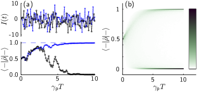
The evolution of and during the measurement process is exemplified in Fig. 2. For now we focus on the qualitative features and we defer a discussion of the specific physical parameters to our detailed presentation of results in Sec. IV. In panel (a) two instances of the simulations have been shown; one which collapses into (blue crosses), and one which does not (black circles). Despite the fact that the two photo-current examples are both quite noisy, they do contain enough information in order to increase the knowledge of the singlet-state overlap, which eventually becomes zero or unity as shown in the lower part of panel (a). In panel (b) the singlet-state-overlap distribution is shown versus time (based on 10,000 simulations). This overlap is initialized at 50% but soon attains a much broader distribution. However, after few times of measurement, the overlap-distribution bifurcates into sharp peaks at zero and unity. Hence, for a sufficiently long measurement time the continuous evolution of effectively facilitates the desired wave-function collapse.
The optimal entanglement-generating protocol simply uses to check to which degree the singlet state, , has been realized. By requiring a minimum value, , for the state overlap, the acceptance criterion for a given quantum state then becomes .
III.3 Practical strategy for entanglement generation
The optimal strategy discussed above requires knowledge of all the physical parameters, , , , , , , , in addition to sufficient data processing capability. This is indeed possible but might be impractical in reality, and hence some more robust but less accurate procedures for establishing whether the singlet state has been prepared are desired. To this end we shall consider the two integrated, dimensionless measurement signals:
| (10) | ||||
| (11) |
In experiment, the former of these corresponds to a simple integration of the photo-current, while the latter corresponds to inserting the photo-current signal into a lock-in amplifier with demodulation frequency, , and time constant, , and integrating for the measurement time, , the squared modulus-output value, ( and are the measured in-phase and in-quadrature amplitudes of the signal at frequency, ). Now, our task is to devise conditions, e.g., or , to accept the quantum state as being sufficiently close to . When simulating the entire entanglement-generating process, the procedure is repeated times, and if of these simulation runs lead to acceptance of the quantum state, we define the success probability as . At the same time, the fidelity measures the average occupation of the spin-singlet state for the generated quantum states, where the sum runs over the accepted density matrices, , simulated by the master equation (1). In principle, it should be possible to reach with (since the initial state has a 50% overlap with ). However, in practice a finite measurement time, qubit decoherence, and a non-optimal extraction of information from reduces the fidelity obtained at a given . An acceptance criterion is well-chosen if both and attain high values.
IV Entanglement generation in absence of qubit decay
This section is devoted to the generation of the spin-singlet state in absence of qubit-population and qubit-phase decay as modeled by the decay operators , i.e. we take , . This simplifies the introduction of all the detailed concepts in the measurement scheme and defines the limits imposed solely by the measurement setup and by the chosen acceptance criteria. The influence of qubit decay is discussed in Sec. V.
In the numerical simulations the stochastic part of Eq. (1) is integrated by the Milstein formula [22], and is evolved using time steps, , being times the characteristic decay time or oscillation time of the physical variables. By repeating the simulations 10,000 times, the statistical spread on fidelity estimates is of the order of one percent.
Without loss of generality, the phase of the driving field, , can be chosen such that and are real. We shall also take , i.e. must then be real. By taking and (i.e. the entire cavity decay takes place through the right-hand mirror in Fig. 1) the effective quantum efficiency, , corresponds to that of the detector, . In experiment such a mirror asymmetry is not necessarily realistic, but adding a homodyne detection setup to the left-hand mirror output and combining the knowledge from all measurements would re-establish , and hence the choice just simplifies the simulations while maintaining the experimental realism. The narrow qubit linewidth calls for , and the correlated decay rate becomes . In the remaining part of this manuscript, all rates are measured relative to and time is measured in units of . For the simulations we take specifically and , such that ensures the validity of the adiabatic elimination.
IV.1 Measurement schemes
IV.1.1 DC-analysis of the photo-current

Following the strategy presented in Sec. III.3, we consider first the use of the photo-current mean value signal from Eq. (10) for distinguishing between the singlet state and the triplet space. According to Eq. (8) it is feasible to choose the local oscillator phase, , such that does not contain a background contribution from the cavity field (note ). The ensemble average of Eq. (10) then becomes:
| (12) |
where the triplet-space steady-state value of is predicted to be (details given in Appendix A):
| (13) |
and the approximation assumes that corresponds to most of the time, i.e. . For the singlet state the -correlated nature of leads to the variance, , while the distribution is broader for the triplet space due to temporal variations in (see Fig. 3(b) and the discussion below). Despite the crudeness of the approximation in Eq. (12) it is clear from the above discussion that an effective distinction between the singlet- and triplet-spaces is possible when , and that the parameters, and , should be optimized in order to maximize according to Eq. (13). When , the maximum value of Eq. (13) is obtained when (see also Fig. 4(c)).
Now, consider Fig. 3 exemplifying the entanglement-generating process. In panel (a) the integrated photo-current, , of Eq. (10) has been plotted for the two individual simulation runs, which were already discussed in Fig. 2(a). As time evolves, the black-circled curve shows an increasing value of , which reflects the fact that the photo-current, (black circles), in the upper part of Fig. 2(a) has a mean value slightly below zero as a consequence of being non-zero for a triplet-state simulation instance. In contrast, in Fig. 2(a) the photo-current (blue crosses) representing a simulation instance ending up in the singlet state is closer to zero on average, which again is reflected in the measurement signal (blue crosses) in Fig. 3(a). Now, the practical acceptance criterion consists simply of keeping a given state provided that ends up at time between the red-dotted lines in Fig. 3(a), i.e. if for a pre-selected value of .
Using the entire set of simulations, the distribution of has been plotted in panel (b) showing a clear double-peak structure. By distinguishing between high () and low () overlap with , we clearly see that each peak corresponds to either the singlet or triplet space. The solid lines are Gaussian functions with unit variance (the shot-noise level of the homodyne-detection procedure) and mean values predicted by the crude approximation of Eq. (12). The singlet-state (crosses) is modeled accurately since is exact and the only variation arises from the random shot noise of the measurement. However, for the triplet state the simulated distribution is evidently broader and asymmetric — the additional width arises from the qubit dynamic evolution within the triplet-state manifold leading to a variation in . Again, the red-dotted lines depict the acceptance window, which clearly selects most of the singlet-state events; however, a small fraction of the undesired triplet-state occurrences are also included. This effect illustrates the fact that the experimentally simple acceptance criterion, , is less accurate than the complete calculation of discussed in Sec. III.2. In fact, if the optimal method of accepting states with for some selected value of is used the undesired instances from the triplet space with poor singlet-state overlap would simply not occur.
The value of and can be calculated as a function of , i.e. for various widths of the acceptance window, as shown in panel (c). Clearly, for small, increasing values of the success probability grows quickly without much degradation in fidelity since the acceptance window selects predominantly the states with a high singlet-state overlap. When the 50-percent success probability is reached, a further increase of must incorporate some triplet-state instances with a loss of fidelity as a result. These observations can also be shown as an -versus- plot, see panel (d). Here the ultimate limit (shown by a blue-dashed line) can be obtained if the singlet- and triplet-spaces present distribution functions like those of panel (b) but being entirely separate.
The fidelity obtained at 50% success probability is shown in Fig. 4(a) for various values of and . The variation in this fidelity can then be compared to the triplet-state steady-state mean value, , which has been plotted in Fig. 4(c) for the same parameter settings of and . The correlation between these figures is evident, which confirms the simple picture discussed around Eq. (12) that the triplet-state imprint onto the photo-current must be maximized for optimizing the performance of the protocol.

IV.1.2 AC-analysis of the photo-current

The spectrum of the photo-current is defined as:
| (14) |
which generally depends on the time, , in the initial transient regime but is time-independent in steady state. For the singlet state the spectrum is flat, , corresponding to the shot noise level of the homodyne detection apparatus. The triplet space is distinguished from the singlet state by identifying a spectral peak in this flat background. In similarity with the expectations discussed around Eq. (12) for the DC-analysis, we shall here use the steady-state spectrum of the triplet space to predict the optimization of , , , and for best performance of the measurement signal, . As a first step, consider the dynamical mean-value equations for , which follow immediately from Eqs. (18)-(20) with being real:
| (15) |
where the coherent driving vector is given by , and the -term (with quadratic -components left out for clarity) tends to drive toward the vector , i.e., the state . The modulation of the photo-current, through and according to Eq. (8), is largest when the spin vector is allowed to sweep across the full sphere, i.e. we expect that is a good choice in order to maintain a significant level of excitation. We note from the expression of that will primarily be spinning around the -axis, which leads to significant oscillations in . For this reason, the local-oscillator-phase choice, , is natural. The oscillations in are then superposed on a constant background level .
The spectrum of the simulated current, where runs over the discrete times separated by , can be conveniently estimated by the periodogram
| (16) |
which is essentially the modulus square of the discrete Fourier transform of . The front factor ensures the correct value, , for the shot noise background, and we subtract from the constant contribution of the bare cavity prior to insertion into .
Turning to the simulation, Fig. 5(a) shows the simulated spectrum for the subset of instances, which collapse into the triplet space, in comparison to the expectation from Eq. (14), which in steady state is given by Eq. (25). Since the integration time, , is significantly larger than unity, this steady-state expression does in fact match the simulated curve very well. In the limit, , numerical inspection of Eq. (25) reveals a Lorentzian peak centered around the generalized Rabi frequency, , and with full-width at half maximum (FWHM) (for the solid curve in Fig. 5(a), the maximum is placed at with ). In order to distinguish between the singlet- and triplet-space part of the initial state, , we must establish the absence or presence of this spectral peak in each individual simulation run. To this end, the lockin parameters of Eq. (11) are chosen as and , and as can be seen from Fig. 5(b), the measurement signal, , is indeed capable of separating the singlet state from the triplet space. The robustness of this procedure to errors in the lockin parameters is depicted in Fig. 5(c,d), which show that must obviously match the position of the spectral peak with an accuracy set by and that provides the best match to the bandwidth of the signal peak. The obtained fidelity and success probability while varying the acceptance criterion, , can be seen in Fig. 5(e,f). These graphs are quite similar to the corresponding results for the DC-measurements in Fig. 3(c,d); however, if a low success probability is accepted, the obtained fidelity seems to be better.
The optimization of the qubit-driving parameters, and , are examined in Fig. 4(b,d). Panel (b) shows the obtained fidelity in various simulations runs, and there is a clear correlation with the calculated spectral-peak height of shown in panel (d). In similarity with the DC-analysis in Sec. IV.1.1, the present AC-analysis of is optimized in terms of and simply by maximizing the triplet-state steady-state spectral peak height, and Fig. 4(d) presents the practical condition, , for this optimization.
IV.2 Practical versus optimal extraction of information

In Fig. 6 the performance of the DC-analysis of as described in Sec. IV.1.1 (solid triangles) can be directly compared to an optimal extraction of information from the full (solid circles) given the local-oscillator phase, . Likewise, the lockin-based AC-analysis of [Sec. IV.1.2] shown with open triangles can be related to an optimal information extraction (open circles) given the phase choice, . In comparison to the optimal extraction of information, the simple and more robust approaches require approximately twice the time for obtaining a given fidelity with a given success rate.
For the DC-analysis protocol the detection record during the initial transient dynamics of duration does not bear much information since neither the singlet- nor triplet-space part of gives rise to a non-zero value of in the initial time range, , in which the two qubit spins are pointing in opposite directions. Hence, by weighting the integral in Eq. (10) by the function , we do not loose information but a smaller amount of shot noise is accumulated in this transient part of the protocol. Combining this weighting procedure with an acceptance window shifted by 0.5 toward the right in Fig. 3(b), we obtain the improved fidelities shown by solid squares in Fig. 6, and the DC-analysis protocol narrows in on the full calculation of .
The AC-analysis protocol is based on the correlation function (9), which contains quadratic moments of and hence is able to deliver an oscillatory signal starting already from . Considering Fig. 6, we ascribe this fact as the reason for the slightly better performance of spin-precession-based protocols (open symbols) in comparison to the spin-mean-value-based protocols (solid symbols) at short integration times.
V The influence of decoherence processes

This section estimates the effect of decoherence processes on the obtainable fidelity. We note that if such processes are strong, the optimum parameter settings as exemplified by Fig. 4 might change. Instead of performing a full-scale analysis of such possible changes, we simply add decoherence processes but keep the measurement protocols and acceptance criteria. The analysis presents a lower bound of the obtainable fidelities an must be a good approximation in the limit of high fidelities. Only the local-oscillator-phase choice of relevant for the DC-analysis protocol is discussed below — the case of presents similar features.
To exemplify the simulation procedure, a qubit-population decay is introduced in Fig. 7(a) with varying values of (modeled by the decay operators and in Sec. III). Since the decay process deteriorates the desired singlet state in the long-integration-time limit there exists an optimum integration time and a corresponding optimum fidelity. This fidelity has been plotted in Fig. 7(b) — see the figure caption for simulation details. In a similar manner, the effect of qubit phase decay can be modeled by assigning a finite value to in the operators and . Furthermore, one may consider the case that the two qubits are not coupled in the exact same way to the cavity. A small inhomogeneity in the coupling strength for each qubit, and , will lead to a slight difference in resonant Rabi frequency, , or alternatively, a small difference in qubit resonance frequency, , could be present. The effect of these non-ideal scenarios are compared in Fig. 7(b) showing that qubit population decay (red squares) and dephasing (green circles) behave in approximately the same way, while the inhomogeneities in Rabi frequency (blue triangles) or qubit detuning (black diamonds) follow their own distinct trend. These observations can be complemented by the equations of motion for the singlet-state population (only the deterministic part, i.e. take ):
| (17) |
Evidently, the two rates and enter on the same footing and are responsible for the de-population of the singlet state. In the high-fidelity limit (, ) one would expect the infidelity, , to increase linearly with these rates. Likewise, the inhomogeneities parametrized by and seem to be comparable in effect — they attempt to drive coherently the population from the singlet state toward (the -term) or (the -term). In the high-fidelity limit the coherence terms, , and , must be polarized before the singlet-state population can be driven, and hence the infidelity is expected to increase quadratically with or . In order to exemplify these scaling behaviors, consider the red squares and blue triangles of Fig. 7(b), which have been re-plotted in panels (c) and (d), respectively. These data scale roughly as the solid lines, which in the double-logarithmic plots have slopes and in panels (c) and (d), respectively. This does not correspond to the scaling behavior discussed above; however, by accepting a smaller success probability, the fidelity increases and the expected scaling is found in the high-fidelity limit. In fact, for the best case shown in panel (c) with optimal information extraction and (solid red diamonds), the infidelity becomes, . At first glance this is surprising since the integration time for obtaining high fidelities is typically exceeding as exemplified in panel (a); however, the infidelity-penalty is not exceeding but is equal to roughly one unit of . A thorough examination of the continuous measurement process in the high-fidelity limit is required to explain this observation: Consider panels (e,f) based on 10,000 simulations in presence of qubit-population decay and using the singlet-state as the initial state, i.e. at . Panel (e) shows the distribution of for various times, which is seen to increase in width during the first few but then settles to an almost constant distribution (compare red squares and black diamonds). However, a sharp feature is emerging around showing an increasing population within the triplet space. Now, the ensemble mean value of based on these distributions is calculated and plotted in panel (f) (blue crosses). The dynamics of this ensemble mean value is governed simply by the deterministic part of the master equation (1) (since ) which for the -component is given by Eq. (17). In the high-fidelity limit the presence of population decay leads to , the solution of which is the solid line in panel (f) confirming the simulations. Nonetheless, the distribution is strongly peaked around zero and unity. In comparison, a drastically different sub-ensemble mean value of can be obtained if we are able to select the best singlet-state candidates. For instance, by conditioning the sub-ensemble on , the green circles are obtained in panel (f). Furthermore, the most probable value of (i.e. the maximum location of the distributions in panel (e)) turns out as the red squares in panel (f). Clearly, after a few times these conditioned observables settle to a steady value. This does not contradict the fact that the state is decaying — the fraction of states with is decreasing steadily as shown by black diamonds in panel (f). To re-capitulate the above discussion: Once the singlet state has been established the continuous measurement either preserves it with a high fidelity or the state jumps into the triplet space. Since the characteristic time for updating our knowledge is , the infidelity of the preserved singlet state is approximately , which explains the steady value of the red squares in panel (f) and the observed dashed-line scaling in panel (c) (since exactly the very best states are selected in this case). A similar set of arguments can be made for the high-fidelity limit in panel (d) for the case of inhomogeneous cavity-qubit coupling, and we note in both cases that the dashed-line slope is in general maintained also for the DC-analysis-based acceptance criterion, . We note that by selecting the best states (in particular when using the optimal extraction of information) the observed infidelity is determined by the ability of the measurement to preserve the state and not sensitive to the statistics of the finite number of simulations.
In the cases of qubit-population or phase decay, the product is essentially equal to (up to factors of two) the cooperativity parameter , where . In the limit of maximum success probability, , the above observations conclude that , which is similar to the figure of merit for deterministic protocols of cavity QED [23]. The measurement process seems to counteract effectively the loss of coherence inherent in the bad-cavity limit, and by accepting a moderately lower success probability, the states with an infidelity of can be conditionally prepared. An infidelity scaling as was also obtained in the heralded protocol of Ref. [23].
VI Discussion
From a fundamental perspective, the correlated decay with rate is the key mechanism for the entanglement-generation protocols. The original product state with opposite qubit-spins gives rise to a 50% overlap with , which allows the measurement process to induce a collapse into the desired singlet state with a high success probability. However, the information of the two-qubit state must be transferred to the cavity field and subsequently leave the cavity before reaching the homodyne-detection apparatus, and it is exactly the decay rate, , which describes the combined rate of this information flow. When the cavity field is adiabatically eliminated the decay rate, , materializes explicitly as a strength parameter in the homodyne-detection photo-current, see e.g. Eqs. (8) and (9). Hence, in our analysis it does not make sense to consider the particular case of (as was done in Figs. 2 and 3 of Ref. [12]) since no information is gained by the measurement.
Even though the measurement process is continuous, the discussion in Sec. V revealed an effective jump-like behavior of the quantum state, and we also remind that discreteness is regained in the long-integration-time limit as exemplified clearly by Fig. 2. These observations are not only of fundamental importance — the detection signal effectively monitors any unwanted transitions into the triplet space. A simple feedback can thus be implemented in order to establish and maintain a high spin-singlet overlap in a continuous operating mode of the experiment. We imagine that a continuous feedback strategy along the lines of Ref. [16] can be developed taking into account the known imprint of the triplet-state components onto the photo-current.
The entanglement-generation protocol relies heavily on the fact that the -state does not couple to the cavity field and the interaction with the field effectively implements a QND measurement [24] of the projection operator . This apparent QND character of the protocol does not rely on the adiabatic elimination and the protocol should be applicable outside the bad-cavity limit. However, the optimization considerations of Sec. IV and the fidelity analysis of Sec. V require the adiabatic approximation to be valid.
VII Conclusion
A measurement-based entanglement-generating protocol has been established for two qubits residing in a bad cavity. The separation of an initial state into either the singlet or triplet space facilitates the establishment of entanglement, which is done optimally by a stochastic-master-equation approach. In addition, two practical methods have been discussed: (1) The use of the integrated photo-current mean value and (2) a lock-in-based identification of oscillations in the photo-current. The optimization of these methods for best performance can be understood simply as maximizing the imprint of the triplet-space part onto the photo-current. The influence of qubit dissipation and inhomogeneities has been analyzed such that obtainable fidelities can be estimated from relevant experimental parameters.
Acknowledgements.
The authors acknowledge support from the EU integrated project AQUTE and the EU 7th Framework Programme collaborative project iQIT.Appendix A Steady-state properties of the triplet space
In this appendix the photo-current, , and its spectrum, , is calculated under the assumption that the two qubits have reached steady state and also assuming that qubit-decay processes are absent (, ). Under the latter assumption the singlet and triplet spaces are decoupled and we consider here only the three-dimensional triplet space. We shall also ignore the information gain from the photo-current (i.e. leaving out the measurement-super-operator part of Eq. (1)) in order to establish an a-priori prediction of the photo-current.
Considering the master equation with the choices made above, the dynamical equations for mean values of , , and read (with real and neglecting the last, Stark-shift term of Eq. (6)):
| (18) | ||||
| (19) | ||||
| (20) | ||||
In Eq. (20) the second line is valid in the special case of the triplet space since the two operators and act identically on the triplet-state basis set: , , , for . We note from all three equations above that the right-hand sides contain mean values of the quadratic operators, , , and , and to proceed the time-derivative of these mean values must be calculated. In turn, cubic operators are introduced and the set of equations seems endless. However, as exemplified above for Eq. (20), by employing operator identities valid in particular for the triplet space, the equations become closed within an eight-dimensional space (corresponding to the number of free parameters in the triplet-space density matrix). Considering the column vector of mean-values: , the dynamical equations become after some algebra:
| (21) |
where the matrix, , and the column vector, , are given by:
| (22) |
The steady-state value of is now simply given by , and since the result of Eq. (13) follows after some algebra.
Turning to the spectrum, , of the photo-current as defined in Eq. (14), we note that correlation functions between and are required according to Eq. (9). To this end, define first a new vector:
| (23) |
i.e. this is the vector evaluated at and multiplied by inside the mean value brackets . According to the quantum regression theorem, the time-evolution of for follows the exact same equation as , i.e. , which has the solution:
| (24) |
where . The first two entries of are equal to and , respectively, which (together with their complex conjugates) are exactly the terms required in Eq. (9). Since in steady state, , the spectrum can be calculated conveniently as an integral over :
| (25) |
with , , and defined as
| (26) |
In the second line of Eq. (25) the row-vector, , extracts the two first entries of and multiplies these by the appropriate weights according to Eq. (9). In the third line the solution (24) is used and the -integration of is carried out. The last line includes (in similarity with the discussion below Eq. (20)) the re-expression of the quadratic and cubic terms of by the linear and quadratic terms of (in steady state) as a particular property of the triplet space: .
For completeness, we present a single-qubit version of the above results in the more general case that decoherence processes and the Stark-shift term of Eq. (6) are included. The vectors , , and are restricted to the first three terms only, and the correlated-decay operator reduces to presenting effectively an extra qubit-population decay channel. The last line of Eq. (25) remains valid when replacing:
| (27) |
where with , and . The single-qubit version of Eq. (13) becomes:
| (28) |
References
- [1] E. Hagley, X. Maître, G. Nogues, C. Wunderlich, M. Brune, J. M. Raimond, and S. Haroche, Phys. Rev. Lett. 79, 1 (1997).
- [2] C. A. Sackett, D. Kielpinski, B. E. King, C. Langer, V. Meyer, C. J. Myatt, M. Rowe, Q. A. Turchette, W. M. Itano, D. J. Wineland, and C. Monroe, Nature 404, 256 (2000).
- [3] F. Schmidt-Kaler, H. Häffner, M. Riebe, S. Gulde, G. P. T. Lancaster, T. Deuschle, C. Becher, C. F. Roos, J. Eschner, and R. Blatt, Nature 422, 408 (2003).
- [4] D. Leibfried, B. DeMarco, V. Meyer, D. Lucas, M. Barrett, J. Britton, W. M. Itano, B. Jelenkovi, C. Langer, T. Rosenband, and D. J. Wineland, Nature 422, 412 (2003).
- [5] M. Ansmann, H. Wang, R. C. Bialczak, M. Hofheinz, E. Lucero, M. Neeley, A. D. O’Connell, D. Sank, M. Weides, J. Wenner, A. N. Cleland, and J. M. Martinis, Nature 461, 504 (2009).
- [6] L. DiCarlo, J. M. Chow, J. M. Gambetta, L. S. Bishop, B. R. Johnson, D. I. Schuster, J. Majer, A. Blais, L. Frunzio, S. M. Girvin, and R. J. Schoelkopf, Nature 460, 240 (2009).
- [7] B. Julsgaard, A. Kozhekin, and E. S. Polzik, Nature 413, 400 (2001).
- [8] C. W. Chou, H. de Riedmatten, D. Felinto, S. V. Polyakov, S. J. van Enk, and H. J. Kimble, Nature 438, 828 (2005).
- [9] D. L. Moehring, P. Maunz, S. Olmschenk, K. C. Younge, D. N. Matsukevich, L.-M. Duan, and C. Monroe, Nature 449, 68 (2007).
- [10] H. J. Kimble, Physica Scripta T76, 127 (1998).
- [11] K. Jacobs and D. A. Steck, Contemp. Phys. 47, 279 (2006).
- [12] C. L. Hutchison, J. Gambetta, A. Blais, and F. Wilhelm, Can. J. Phys. 87, 225 (2009).
- [13] H. M. Wiseman and G. J. Milburn, Phys. Rev. A 47, 642 (1993).
- [14] M. J. Collett and C. W. Gardiner, Phys. Rev. A 30, 1386 (1984).
- [15] B. Julsgaard and K. Mølmer, Phys. Rev. A 85, 013844 (2012).
- [16] J. Wang, H. M. Wiseman, and G. J. Milburn, Phys. Rev. A 71, 042309 (2005).
- [17] E. M. Purcell, Phys. Rev. 69, 681 (1946).
- [18] Y. Kubo, F. R. Ong, P. Bertet, D. Vion, V. Jacques, D. Zheng, A. Dreau, J. F. Roch, A. Auffeves, F. Jelezko, J. Wrachtrup, M. F. Barthe, P. Bergonzo, and D. Esteve, Phys. Rev. Lett. 105, 140502 (2010).
- [19] D. I. Schuster, A. P. Sears, E. Ginossar, L. DiCarlo, L. Frunzio, J. J. L. Morton, H. Wu, G. A. D. Briggs, B. B. Buckley, D. D. Awschalom, and R. J. Schoelkopf, Phys. Rev. Lett. 105, 140501 (2010).
- [20] R. Amsüss, C. Koller, T. Nöbauer, S. Putz, S. Rotter, K. Sandner, S. Schneider, M. Schramböck, G. Steinhauser, H. Ritsch, J. Schmiedmayer, and J. Majer, Phys. Rev. Lett. 107, 060502 (2011).
- [21] S. Olmschenk, K. C. Younge, D. L. Moehring, D. N. Matsukevich, P. Maunz, and C. Monroe, Phys. Rev. A 76, 052314 (2007).
- [22] P. E. Kloeden and E. Platen, Numerical solution of stochastic differential equations (Springer-Verlag, Heidelberg, 1992).
- [23] A. S. Sørensen and K. Mølmer, Phys. Rev. Lett. 91, 097905 (2003).
- [24] V. B. Braginsky and F. Y. Khalili, Rev. Mod. Phys. 68, 1 (1996).