跳到论文正文
W Papers独立论文阅读器 arXiv:1202.4736 论文正文 计算阅读时间 · 0%
引用这篇论文根据当前论文元数据生成,正式投稿前建议核对。


License: arXiv.org perpetual non-exclusive license
arXiv:1202.4736v2 [cs.IT] 23 Feb 2012

Diversity of MIMO Linear Precoding

Ahmed Hesham Mehana    Aria Nosratinia ††thanks: The authors are with the Department of Electrical Engineering, The University of Texas at Dallas, Richardson, TX 75083-0688 USA, E-mail: ahmed.mehana@student.utdallas.edu; aria@utdallas.edu.
Abstract

Linear precoding is a relatively simple method of MIMO signaling that can also be optimal in certain special cases. This paper is dedicated to high-SNR analysis of MIMO linear precoding. The Diversity-Multiplexing Tradeoff (DMT) of a number of linear precoders is analyzed. Furthermore, since the diversity at finite rate (also known as the fixed-rate regime, corresponding to multiplexing gain of zero) does not always follow from the DMT, linear precoders are also analyzed for their diversity at fixed rates. In several cases, the diversity at multiplexing gain of zero is found not to be unique, but rather to depend on spectral efficiency. The analysis includes the zero-forcing (ZF), regularized ZF, matched filtering and Wiener filtering precoders. We calculate the DMT of ZF precoding under two common design approaches, namely maximizing the throughput and minimizing the transmit power. It is shown that regularized ZF (RZF) or Matched filter (MF) suffer from error floors for all positive multiplexing gains. However, in the fixed rate regime, RZF and MF precoding achieve full diversity up to a certain spectral efficiency and zero diversity at rates above it. When the regularization parameter in the RZF is optimized in the MMSE sense, the structure is known as the Wiener precoder which in the fixed-rate regime is shown to have diversity that depends not only on the number of antennas, but also on the spectral efficiency. The diversity in the presence of both precoding and equalization is also analyzed.

I Introduction

Precoding is a preprocessing technique that exploits channel-state information at the transmitter (CSIT) to match the transmission to the instantaneous channel conditions [1, 2, 3]. Linear and non-linear precoding designs are available in the literature [4]. Linear precoding in particular provides a simple and efficient method to utilize CSIT. Linear precoding has been shown to be optimal in certain situations involving partial CSIT [5, 6], however, in many instances the main motivation of linear precoders is to simplify the MIMO receiver.

Linear precoders include zero-forcing (ZF), matched filtering (MF), Wiener filtering, and regularized zero-forcing (RZF). The ZF precoding schemes were extensively studied in multiuser systems as the ZF decouples the multiuser channel into independent single-user channels and has been shown to achieve a large portion of dirty paper coding capacity [7]. ZF precoding often involves channel inversion, using the pseudo-inverse of the channel or other generalized inverses [4]. Matched filter (MF) precoding [8], similarly to the MF receiver, is interference limited at high SNR but it outperforms the ZF precoder at low SNR [4]. The regularized ZF precoder, as the name implies, introduces a regularization parameter in channel inversion. If the regularization parameter is inversely proportional to SNR, the RZF of [9] is identical to the Wiener filter precoding [4]. Peel et al. [9] introduce a vector perturbation technique to reduce the transmit power of the RZF method, showing that in this way RZF can operate near channel capacity.

This paper analyzes the diversity of MIMO linear precoding with or without linear receivers. We show that a MIMO ZF precoder with a maximum likelihood receiver has minimal spatial diversity, and that Wiener precoders produce a diversity that is a complex function of spectral efficiency and the number of transmit and receive antennas. At very low rates, the Wiener precoder enjoys a maximal diversity which is the product of the number of transmit and receive antennas, while at very high rates it achieves a minimal diversity which is the same as ZF diversity. These results are reminiscent of MIMO linear equalizers [10], even though in general the behavior of equalizers (receive side) can be very different from precoders (transmit side) and the analysis does not carry from one to the other. We also show that MIMO systems with RZF and MF precoders (together with optimal receivers) exhibit a new kind of rate-dependent diversity that has not to date been observed or reported, i.e., they either have full diversity or zero diversity (error floor) depending on the operating spectral efficiency RR.

We also provide DMT analysis for all precoders mentioned above. The fact that DMT and the diversity under fixed-rate regime require separate analyses has been established for MIMO linear equalizers [11, 10] and is by now a well-understood phenomenon. Essentially, the reason is that various fixed rates (spectral efficiencies) for MIMO precoding result in distinctly different diversities, whereas DMT analysis assigns only a single value of diversity to all fixed rates (all fixed rates correspond to multiplexing gain zero).

Remark 1

Due to symbolic similarities, it may be tempting to draw the conclusion that if d⁡(r)d(r) is the diversity at multiplexing gain rr, then substituting r=0r=0 in the same mathematical expression will give the diversity at multiplexing gain zero d⁡(0)d(0). However, despite appearances, there is no solid relationship between d⁡(r)d(r) and d⁡(0)d(0). The standard DMT arguments are based on the seminal work of Zheng and Tse [12] whose developments depend critically on the positivity of rr. For example, the proof of [12, Lemma 5] depends critically on rr being strictly positive.More importantly, the asymptotic outage calculations in [12, p. 1079] implicitly use r>0r>0 and result in the outage region:

𝒜={α:∑i(1−αi)+<r}{\mathcal{A}}=\{\alpha:\sum_{i}(1-\alpha_{i})^{+}<r\}

where αi\alpha_{i} are the exponential order of the channel eigenvalues, i.e., λi=ρ−αi\lambda_{i}=\rho^{-\alpha_{i}}. If we set r=0r=0 this expression implies that the outage region is always empty, which is clearly not true.

Thus, the DMT as calculated by the standard methods of [12] does not extend to r=0r=0. The DMT d⁡(r)d(r) is sometimes continuous at zero, including e.g. the examples in [12], but continuity at r=0r=0 does not always hold. In fact, there are systems where d⁡(0)d(0), the diversity at multiplexing gain zero, is not even uniquely defined. It is possible for diversity to take multiple values as a function of rate RR. This fact has been observed and analyzed, e.g., in [11, 10, 13]. The work in the present paper also produces several examples of this phenomenon.

This paper is organized as follows. Section II describes the system model. Section III provides outage analysis of many precoded MIMO systems. Section IV provides the DMT analysis. The case of joint linear transmit and receive filters is discussed in Section V. Section VI provides simulations that illuminate our results.
Refer to caption
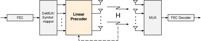
Fig. 1: MIMO with linear precoder

II System Model

A MIMO system with linear precoding is depicted in Fig. 1. This system uses the linear precoder to manage the interference between the streams in a MIMO system to avoid a lattice decoder in the receiver. We consider a flat fading channel 𝐇∈ℂN×M{\mathbf{H}}\in\mathbb{C}^{N\times M}, where MM and NN are the number of transmit and receive antennas, respectively. While M⩾NM\geqslant N when using linear precoding alone, we have N⩾MN\geqslant M or M⩾NM\geqslant N when using precoding together with receive-side linear equalization depending on whether the precoder is designed for the equalized channel or the equalizer is designed for the precoded channel (see Figure 2). The input-output system model for flat fading MIMO channel with MM transmit and NN receive antennas is given by

𝐲=𝐖𝐇𝐓𝐱+𝐖𝐧{\mathbf{y}}={\mathbf{W}}{\mathbf{H}}{\mathbf{T}}{\mathbf{x}}+{\mathbf{W}}{\mathbf{n}} (1)

where 𝐓∈ℂM×B{\mathbf{T}}\in\mathbb{C}^{M\times B} is the precoder matrix, 𝐖∈ℂB×N{\mathbf{W}}\in\mathbb{C}^{B\times N} is the receiver side equalizer. The latter may be set to identity in cases where the receiver does not use linear equalization. The number of information symbols is B⩽min⁡(M,N)B\leqslant\min(M,N), the transmitted vector is 𝐱∈ℂB×1{{\mathbf{x}}\in\mathbb{C}^{\ B\times 1}}, and 𝐧∈ℂN×1{{\mathbf{n}}\in\mathbb{C}^{\ N\times 1}} is the Gaussian noise vector. The vectors 𝐱{{\mathbf{x}}} and 𝐧{{\mathbf{n}}} are assumed independent.

We aim to characterize the diversity gain, d⁡(R,M,N)d(R,M,N), as a function of the spectral efficiency RR (bits/sec/Hz) and the number of transmit and receive antennas. This requires a Pairwise Error Probability (PEP) analysis which is not directly tractable. Instead, we find the exponential order of outage probability and then demonstrate that outage and PEP exhibit identical exponential orders.

The objective of linear precoding (possibly together with linear equalization at the receiver) is to transform the MIMO channel into min⁡(M,N)\min(M,N) parallel channels that can be described by

yk=γkxk+nk,k=1,…,By_{k}=\sqrt{\gamma_{k}}x_{k}+n_{k},\quad k=1,\dots,B (2)

where γk\gamma_{k} is the SINR at the kk-th receiver output and B=m​i​n​(M,N)B=min(M,N). Following the notation of [14], we define the outage-type quantities

Po​u​t​(R,N,M)\displaystyle P_{out}(R,N,M) ≜ℙ⁡(I⁡(𝐱,𝐲)<R)\displaystyle\triangleq{\mathbb{P}}(I({\mathbf{x}};{\mathbf{y}})<R) (3)
do​u​t​(R,N,M)\displaystyle d_{out}(R,N,M) ≜−limρ→∞log⁡Po​u​t​(R,M,N)log⁡ρ\displaystyle\triangleq-\lim_{\rho\rightarrow\infty}\frac{\log P_{out}(R,M,N)}{\log\rho} (4)

where ρ\rho is the transmitted equivalent SNR.

The outage probabilities of MIMO systems under joint spatial encoding is respectively given by [11, 13]

Pout≜ℙ⁡(∑k=1Blog⁡(1+γk)⩽R)\displaystyle P_{\text{out}}\triangleq{\mathbb{P}}\bigg(\sum_{k=1}^{B}\log(1+\gamma_{k})\leqslant R\bigg) (5)

We shall perform outage analysis for different precoders/equalizers as the first step towards deriving the diversity function. We then provide lower and upper bounds on error probability via outage probabilities. This two-step approach was first proposed in [12] due to the intractability of the direct PEP analysis for many MIMO architectures.

We denote the exponential equality of two functions f⁡(ρ)f(\rho) and g⁡(ρ)g(\rho) as f⁡(p)≐g⁡(p)f(p)\doteq g(p) when

limρ→∞log⁡f⁡(ρ)log⁡(ρ)=limρ→∞log⁡g⁡(ρ)log⁡(ρ)\lim_{\rho\rightarrow\infty}\frac{\log f(\rho)}{\log(\rho)}=\lim_{\rho\rightarrow\infty}\frac{\log g(\rho)}{\log(\rho)}

In the following, we shall need to specify various upper and lower bounds or approximations of the SINR γ\gamma, which will give rise to a number of pseudo-SINR variables γ^\hat{\gamma}, γ˘\breve{\gamma}, and γ¯\bar{\gamma}.

III Precoding Diversity

In this section we analyze a linearly precoded MIMO system where M≥NM\geq N and the number of data streams BB is equal to NN.

III-A Zero-Forcing Precoding

The ZF precoder completely eliminates the interference at the receiver. ZF precoding is well studied in the literature via performance measures such as throughput and fairness under a total (or per antenna) power constraint [15, and references therein].

III-A1 Design Method I

One approach to design the ZF precoder is to solve the following problem [4]

𝐓=\displaystyle{\mathbf{T}}= arg⁡min𝐓⁡𝔼⁡[‖𝐓𝐱‖22]\displaystyle\arg\min_{{\mathbf{T}}}{\mathbb{E}}\big[||{\mathbf{T}}{\mathbf{x}}||^{2}_{2}\big] (6)
subject to ​𝐇𝐓=𝐈\displaystyle\text{subject to }{\mathbf{H}}{\mathbf{T}}={\mathbf{I}}

The resulting ZF transmit filter is given by

𝐓=β​𝐇H​(𝐇𝐇H)−1∈ℂM×N{\mathbf{T}}=\beta\,{\mathbf{H}}^{H}({\mathbf{H}}{\mathbf{H}}^{H})^{-1}\in\mathbb{C}^{M\times N} (7)

where β\beta is a scaling factor to satisfy the transmit power constraint, that is [4]

β2​tr​(𝐓𝐓H)⩽ρ\beta^{2}\text{tr}\big({\mathbf{T}}{\mathbf{T}}^{H}\big)\leqslant\rho (8)

where we assume that the noise power is one and that the information streams are independent. From (8), the received SINR per stream is thus given by

γkZ​F​P=ρtr​(𝐇𝐇H)−1.\gamma^{ZFP}_{k}=\frac{\rho}{\text{tr}({\mathbf{H}}{\mathbf{H}}^{H})^{-1}}. (9)

Using (5), the outage probability is given by

Pout=ℙ⁡(N​log⁡(1+ρtr​((𝐇𝐇H)−1))⩽R)P_{\text{out}}={\mathbb{P}}\bigg(N\log\big(1+\frac{\rho}{\text{tr}(({\mathbf{H}}{\mathbf{H}}^{H})^{-1})}\big)\leqslant R\bigg) (10)

A direct evaluation of (10) is intractable since the diagonal elements of (𝐇𝐇H)−1({\mathbf{H}}{\mathbf{H}}^{H})^{-1} are distributed according to the inverse-chi-square distribution [16, 11]. We instead bound (10) from below and above and show that the two bounds match asymptotically.

Let λk\lambda_{k} be the k-th eigenvalue of 𝐇𝐇H{\mathbf{H}}{\mathbf{H}}^{H}. Equation (10) can be written as

Pout=ℙ⁡(N​log⁡(1+ρ∑k=1N1λk)⩽R)P_{\text{out}}={\mathbb{P}}\bigg(N\log\big(1+\frac{\rho}{\sum_{k=1}^{N}\frac{1}{\lambda_{k}}}\big)\leqslant R\bigg)

which can be bounded as

Pout\displaystyle P_{\text{out}} ⩽ℙ⁡(N​log⁡(1+ρN​λmin)⩽R)\displaystyle\leqslant{\mathbb{P}}\bigg(N\log(1+\frac{\rho}{N}\lambda_{\text{min}})\leqslant R\bigg) (11)
=ℙ⁡(λmin⩽N⁡(2RN−1)​R​ρ−1)\displaystyle={\mathbb{P}}\bigg(\lambda_{\text{min}}\leqslant N(2^{\frac{R}{N}}-1)R\rho^{-1}\bigg)
=˙​ℙ​(λmin⩽ρ−1).\displaystyle\dot{=}\;\,{\mathbb{P}}\big(\lambda_{\text{min}}\leqslant\rho^{-1}\big). (12)

The marginal distribution f1​(λ)f_{1}(\lambda) of λmin\lambda_{\text{min}} is f1​(λ)=c​λ(M−N)f_{1}(\lambda)=c\lambda^{(M-N)} [17] where cc is a constant, therefore the bound in (12) can be evaluated [13] yielding:

Pout​⩽˙​ρ−(M−N+1).P_{\text{out}}\;\dot{\leqslant}\;\;\rho^{-(M-N+1)}. (13)

We now proceed with a lower bound on outage. The outage probability in (10) can be bounded:

Pout\displaystyle P_{\text{out}} =ℙ⁡(N​log⁡(1+ρtr​(𝐇𝐇H)−1)⩽R)\displaystyle={\mathbb{P}}\bigg(N\log(1+\frac{\rho}{\text{tr}({\mathbf{H}}{\mathbf{H}}^{H})^{-1}})\leqslant R\bigg)
⩾ℙ⁡(N​log⁡(1+ρ(𝐇𝐇H)k​k−1)⩽R)\displaystyle\geqslant{\mathbb{P}}\bigg(N\log(1+\frac{\rho}{({\mathbf{H}}{\mathbf{H}}^{H})^{-1}_{kk}})\leqslant R\bigg)
=˙​ℙ​(z⩽ρ−1)\displaystyle\dot{=}\;\;{\mathbb{P}}\bigg(z\leqslant\rho^{-1}\bigg) (14)

where we have made a change of variable z=1(𝐇𝐇H)k​k−1z=\frac{1}{({\mathbf{H}}{\mathbf{H}}^{H})^{-1}_{kk}}.

The random variable zz in (14) is distributed according to the chi-square distribution with 2​(M−N+1)2(M-N+1) degree of freedom, i.e. z∼𝒳2​2​(M−N+1)z\sim\mathcal{X}^{2}2(M-N+1) [16]. Thus the bound in (14) can be evaluated [11] yielding:

Pout​⩾˙​ρ−(M−N+1).P_{\text{out}}\;\dot{\geqslant}\;\;\rho^{-(M-N+1)}. (15)

From (13) and (15), we conclude that the diversity of MIMO system using the ZF precoder given by (6) and joint spatial encoding is

dZ​F​P=M−N+1.d^{ZFP}=M-N+1. (16)

III-B Zero-Forcing Precoding: Design Method II

Notice that the ZF precoder design in (6) minimizes the transmitted power. Another approach for ZF precoding design allocates unequal power levels across the transmit antennas to optimize some performance measure. For instance, consider the optimization problem [15]

maxpk,𝐓⁡f⁡(pk)\displaystyle\max_{p_{k},{\mathbf{T}}}\;\;f(p_{k})
subject to𝐇𝐓=diag​{p1,…,pM}\displaystyle\text{subject to}\;\;\;\;\;{\mathbf{H}}{\mathbf{T}}=\text{diag}\{\sqrt{p_{1}},\dots,\sqrt{p_{M}}\}
𝔼​‖𝐓𝐱‖2⩽ρ\displaystyle\hskip 26.0pt{\mathbb{E}}||{\mathbf{T}}{\mathbf{x}}||^{2}\leqslant\rho (17)

where f⁡(pk)f(p_{k}) is an arbitrary function of the transmitted power pkp_{k} on the kk-th antenna.

The optimal solution for (17) (assuming independent transmit signaling) is given by [15, Theorem 1]:

𝐓=𝐇H​(𝐇𝐇H)−1​diag​{p1,…,pM}{\mathbf{T}}={\mathbf{H}}^{H}({\mathbf{H}}{\mathbf{H}}^{H})^{-1}\text{diag}\{\sqrt{p_{1}},\dots,\sqrt{p_{M}}\} (18)

where pkp_{k} is obtained by solving

maxpk⁡f⁡(pk)\displaystyle\max_{p_{k}}\;\;f(p_{k})
subject to∑kpk​[(𝐇𝐇H)−1]k​k⩽ρ\displaystyle\text{subject to}\;\;\;\;\;\sum_{k}p_{k}\big[({\mathbf{H}}{\mathbf{H}}^{H})^{-1}\big]_{kk}\leqslant\rho (19)

In our case, we maximize the throughput, therefore f⁡(pk)=∑klog⁡(1+γkZ​F​P)f(p_{k})=\sum_{k}\log(1+\gamma^{ZFP}_{k}). After setting the derivatives of the appropriate Lagrangian function to zero, the solution of the power allocation problem in (19) is given by

pk=ρ+∑k=1M(𝐇𝐇H)k​k−1M​(𝐇𝐇H)k​k−1−1p_{k}=\frac{\rho+\sum_{k=1}^{M}({\mathbf{H}}{\mathbf{H}}^{H})^{-1}_{kk}}{M({\mathbf{H}}{\mathbf{H}}^{H})^{-1}_{kk}}-1 (20)

Substituting (20) in (5), the outage probability is given by

Pout\displaystyle P_{\text{out}} =ℙ⁡(∑k=1Nlog⁡(ρ+∑k=1N(𝐇𝐇H)k​k−1M​(𝐇𝐇H)k​k−1)⩽R)\displaystyle={\mathbb{P}}\bigg(\sum_{k=1}^{N}\log(\frac{\rho+\sum_{k=1}^{N}({\mathbf{H}}{\mathbf{H}}^{H})^{-1}_{kk}}{M({\mathbf{H}}{\mathbf{H}}^{H})^{-1}_{kk}})\leqslant R\bigg)
=˙​ℙ​(∑k=1Nlog⁡(ρM​(𝐇𝐇H)k​k−1)⩽R)\displaystyle\dot{=}\;\;{\mathbb{P}}\bigg(\sum_{k=1}^{N}\log(\frac{\rho}{M({\mathbf{H}}{\mathbf{H}}^{H})^{-1}_{kk}})\leqslant R\bigg) (21)
=ℙ⁡(∑k=1Nlog⁡(M​(𝐇𝐇H)k​k−1ρ)⩾−R)\displaystyle={\mathbb{P}}\bigg(\sum_{k=1}^{N}\log(\frac{M({\mathbf{H}}{\mathbf{H}}^{H})^{-1}_{kk}}{\rho})\geqslant-R\bigg) (22)
⩽ℙ⁡(N​log​∑k=1N((𝐇𝐇H)k​k−1ρ)⩾−R)\displaystyle\leqslant{\mathbb{P}}\bigg(N\log\sum_{k=1}^{N}(\frac{({\mathbf{H}}{\mathbf{H}}^{H})^{-1}_{kk}}{\rho})\geqslant-R\bigg) (23)
=ℙ⁡(∑k=1N1ρ​λk⩾2−RN)\displaystyle={\mathbb{P}}\bigg(\sum_{k=1}^{N}\frac{1}{\rho\lambda_{k}}\geqslant 2^{-\frac{R}{N}}\bigg)
⩽ℙ⁡(1ρ​λmin⩾1N​2−RN)\displaystyle\leqslant{\mathbb{P}}\bigg(\frac{1}{\rho\lambda_{\text{min}}}\geqslant\frac{1}{N}2^{-\frac{R}{N}}\bigg)\;
≐ℙ⁡(λmin⩽ρ−1)\displaystyle\doteq\;{\mathbb{P}}\bigg(\lambda_{\text{min}}\leqslant\rho^{-1}\bigg) (24)
≐ρ−(M−N+1).\displaystyle\doteq\rho^{-(M-N+1)}. (25)

where the exponential equality (21) holds at high SNR, (23) follows from Jensen’s inequality, and the transition from (24) to (25) again due to the marginal distribution of λmin\lambda_{\min} via the method of [13].

A lower bound on the outage probability can be given as follows. Starting with (21) and using Jensen’s inequality we have

Pout\displaystyle P_{\text{out}} =˙​ℙ​(∑k=1Nlog⁡(ρN​(𝐇𝐇H)k​k−1)⩽R)\displaystyle\dot{=}\;\;{\mathbb{P}}\bigg(\sum_{k=1}^{N}\log(\frac{\rho}{N({\mathbf{H}}{\mathbf{H}}^{H})^{-1}_{kk}})\leqslant R\bigg)
⩾ℙ⁡(N​log⁡1N2​∑k=1Nρ(𝐇𝐇H)k​k−1⩽R).\displaystyle\geqslant{\mathbb{P}}\bigg(N\log\frac{1}{N^{2}}\sum_{k=1}^{N}\frac{\rho}{({\mathbf{H}}{\mathbf{H}}^{H})^{-1}_{kk}}\leqslant R\bigg). (26)

The singular value decomposition of 𝐇{\mathbf{H}} and the corresponding eigen decomposition of 𝐇𝐇H{\mathbf{H}}{\mathbf{H}}^{H} are given by

𝐇=𝐔​Γ​𝐕H\displaystyle{\mathbf{H}}\quad\hskip 6.0pt={\mathbf{U}}\,\Gamma\,{\mathbf{V}}^{H}
𝐇𝐇H=𝐔​Λ​𝐔H\displaystyle{\mathbf{H}}{\mathbf{H}}^{H}={\mathbf{U}}\Lambda\,{\mathbf{U}}^{H}

where 𝐔∈ℂN×N{\mathbf{U}}\in\mathbb{C}^{N\times N} and 𝐕∈ℂM×M{\mathbf{V}}\in\mathbb{C}^{M\times M} are unitary matrices, Γ∈ℝN×M\Gamma\in\mathbb{R}^{N\times M} is a rectangular matrix with non-negative real diagonal elements and zero off-diagonal elements, and Λ=Γ​ΓT∈ℝN×N\Lambda=\Gamma\Gamma^{T}\in\mathbb{R}^{N\times N} is a diagonal matrix whose diagonal elements are the eigenvalues of 𝐇𝐇H{\mathbf{H}}{\mathbf{H}}^{H}. Let 𝐮k{\mathbf{u}}_{k} be the kk-th column of 𝐔H{\mathbf{U}}^{H}. We have

(𝐇𝐇H)k​k−1=𝐮kH​Λ−1​𝐮k=∑l=1N|uk​l|2λl({\mathbf{H}}{\mathbf{H}}^{H})^{-1}_{kk}={\mathbf{u}}^{H}_{k}\Lambda^{-1}{\mathbf{u}}_{k}=\sum_{l=1}^{N}\frac{|u_{kl}|^{2}}{\lambda_{l}} (27)

where uk​lu_{kl} is the (k,l)(k,l) entry of the matrix 𝐔{\mathbf{U}}.

The bound in (26) can be rewritten

Pout\displaystyle P_{\text{out}}\; ⩾˙​ℙ​(N​log⁡1N2​∑k=1N1∑l=1N|uk​l|2ρ​λl⩽R)\displaystyle\dot{\geqslant}\;{\mathbb{P}}\bigg(N\log\frac{1}{N^{2}}\sum_{k=1}^{N}\frac{1}{\sum_{l=1}^{N}\frac{|u_{kl}|^{2}}{\rho\lambda_{l}}}\leqslant R\bigg)
⩾ℙ⁡(N​log⁡1N2​∑k=1N1∑l=1N|uk​l|21+ρ​λl⩽R)\displaystyle\geqslant{\mathbb{P}}\bigg(N\log\frac{1}{N^{2}}\sum_{k=1}^{N}\frac{1}{\sum_{l=1}^{N}\frac{|u_{kl}|^{2}}{1+\rho\lambda_{l}}}\leqslant R\bigg) (28)

We can lower bound the probability in (28) in by observing that the term

1N​∑k=1N1∑l=1N|uk​l|21+ρ​λl\frac{1}{N}\sum_{k=1}^{N}\frac{1}{\sum_{l=1}^{N}\frac{|u_{kl}|^{2}}{1+\rho\lambda_{l}}}

is similar to [13, Eq.(18)], thus the analysis of [13] applies and we obtain

Pout​⩾˙​ℙ​(λmin⩽ρ−1)=ρ−(M−N+1).P_{\text{out}}\;\dot{\geqslant}\;{\mathbb{P}}\bigg(\lambda_{\text{min}}\leqslant\rho^{-1}\bigg)=\rho^{-(M-N+1)}. (29)

Thus, the MIMO ZF precoding with unequal power allocation (19) achieves diversity order M−N+1M-N+1.

Recall that the diversity is defined based on the error probability. In Appendix -A we provide the pairwise error probability (PEP) analysis for the zero-forcing and regularized zero-forcing precoded systems and show that the outage and error probabilities exhibit same diversity.

III-C Regularized Zero-Forcing Precoding

In general, direct channel inversion performs poorly due to the singular value spread of the channel matrix [9]. One technique often used is to regularize the channel inversion:

𝐓=β​𝐇H​(𝐇𝐇H+c​𝐈)−1{\mathbf{T}}=\beta\,{\mathbf{H}}^{H}({\mathbf{H}}{\mathbf{H}}^{H}+c\,{\mathbf{I}})^{-1} (30)

where β\beta is a normalization factor and cc is a fixed constant.

Recall

𝐲=𝐇𝐓𝐱+𝐧\displaystyle{\mathbf{y}}={\mathbf{H}}{\mathbf{T}}{\mathbf{x}}+{\mathbf{n}} =β​𝐔​Λ​(Λ+c​𝐈)−1​𝐔H​𝐱+𝐧\displaystyle=\beta{\mathbf{U}}\Lambda(\Lambda+c\,{\mathbf{I}})^{-1}{\mathbf{U}}^{H}{\mathbf{x}}+{\mathbf{n}} (31)

allowing us to decompose the received waveform at each antenna into signal, interference, and noise terms:

yk\displaystyle y_{k} =β⁡(∑l=1Nλlλl+c​|uk​l|2)​xk+\displaystyle=\beta\bigg(\sum_{l=1}^{N}\frac{\lambda_{l}}{\lambda_{l}+c\,}|u_{kl}|^{2}\bigg)x_{k}\;\;+
β​∑i=1,i≠kN(∑l=1Nλlλl+c​uk​l​ui​l∗)​xi+nk\displaystyle\quad\;\beta\sum_{i=1,i\neq k}^{N}\bigg(\sum_{l=1}^{N}\frac{\lambda_{l}}{\lambda_{l}+c\,}u_{kl}u^{*}_{il}\bigg)x_{i}+n_{k} (32)

where the scaling factor β\beta is given by β=1η\beta=\frac{1}{\sqrt{\eta}} and

η\displaystyle\eta =tr​[(𝐇𝐇H+c​𝐈)−1​𝐇𝐇H​(𝐇𝐇H+c​𝐈)−1]\displaystyle=\text{tr}\big[({\mathbf{H}}{\mathbf{H}}^{H}+c\,{\mathbf{I}})^{-1}{\mathbf{H}}{\mathbf{H}}^{H}({\mathbf{H}}{\mathbf{H}}^{H}+c\,{\mathbf{I}})^{-1}\big]
=tr​[(𝐔​Λ​𝐔H+c​𝐈)−1​𝐔​Λ​𝐔H​(𝐔​Λ​𝐔H+c​𝐈)−1]\displaystyle=\text{tr}\big[({\mathbf{U}}\Lambda{\mathbf{U}}^{H}+c\,{\mathbf{I}})^{-1}{\mathbf{U}}\Lambda{\mathbf{U}}^{H}({\mathbf{U}}\Lambda{\mathbf{U}}^{H}+c\,{\mathbf{I}})^{-1}\big]
=tr​[𝐔​(Λ+c​𝐈)−1​Λ​(Λ+c​𝐈)−1​𝐔H]\displaystyle=\text{tr}\big[{\mathbf{U}}(\Lambda+c\,{\mathbf{I}})^{-1}\Lambda(\Lambda+c\,{\mathbf{I}})^{-1}{\mathbf{U}}^{H}\big]
=tr​[Λ​(Λ+c​𝐈)−2]=∑l=1Nλl(λl+c)2.\displaystyle=\text{tr}\big[\Lambda(\Lambda+c\,{\mathbf{I}})^{-2}\big]=\sum_{l=1}^{N}\frac{\lambda_{l}}{(\lambda_{l}+c\,)^{2}}. (33)

The received signal power is given by

PT\displaystyle P_{T} =E​‖𝐇𝐓𝐱‖2\displaystyle=E||{\mathbf{H}}{\mathbf{T}}{\mathbf{x}}||^{2}
=E⁡[β2​tr​(𝐔​Λ​(Λ+c​𝐈)−1​𝐔H​𝐱𝐱H​𝐔​(Λ+c​𝐈)−1​Λ​𝐔H)]\displaystyle=E\bigg[\beta^{2}\text{tr}\bigg({\mathbf{U}}\Lambda(\Lambda+c\,{\mathbf{I}})^{-1}{\mathbf{U}}^{H}{\mathbf{x}}{\mathbf{x}}^{H}{\mathbf{U}}(\Lambda+c\,{\mathbf{I}})^{-1}\Lambda{\mathbf{U}}^{H}\bigg)\bigg]
=E⁡[β2​tr​(Λ​(Λ+c​𝐈)−1​𝐔H​𝐱𝐱H​𝐔​(Λ+c​𝐈)−1​Λ​𝐔H​𝐔)]\displaystyle=E\bigg[\beta^{2}\text{tr}\bigg(\Lambda(\Lambda+c\,{\mathbf{I}})^{-1}{\mathbf{U}}^{H}{\mathbf{x}}{\mathbf{x}}^{H}{\mathbf{U}}(\Lambda+c\,{\mathbf{I}})^{-1}\Lambda{\mathbf{U}}^{H}{\mathbf{U}}\bigg)\bigg]
=β2​tr​(Λ​(Λ+c​𝐈)−1​𝐔H​E​(𝐱𝐱H)​𝐔​(Λ+c​𝐈)−1​Λ)\displaystyle=\beta^{2}\text{tr}\bigg(\Lambda(\Lambda+c\,{\mathbf{I}})^{-1}{\mathbf{U}}^{H}E({\mathbf{x}}{\mathbf{x}}^{H}){\mathbf{U}}(\Lambda+c\,{\mathbf{I}})^{-1}\Lambda\bigg)
=β2​ρN​tr​[(Λ+c​𝐈)−2​Λ2]=β2​ρN​∑l=1Nλl2(λl+c)2.\displaystyle=\frac{\beta^{2}\rho}{N}\text{tr}\big[(\Lambda+c\,{\mathbf{I}})^{-2}\Lambda^{2}\big]=\frac{\beta^{2}\rho}{N}\sum_{l=1}^{N}\frac{\lambda_{l}^{2}}{(\lambda_{l}+c\,)^{2}}. (34)

where we have used 𝔼⁡(𝐱𝐱H)=ρN​𝐈{\mathbb{E}}({\mathbf{x}}{\mathbf{x}}^{H})=\frac{\rho}{N}{\mathbf{I}}.

The SINR is evaluated by computing the signal and interference powers from (32). For a given channel 𝐇{\mathbf{H}}, the power of desired and interference signals at the kk-th receive antenna are respectively given by

PD(k)\displaystyle P^{(k)}_{D} =β2​ρN​(∑l=1Nλlλl+c​|uk​l|2)2\displaystyle=\frac{\beta^{2}\rho}{N}\bigg(\sum_{l=1}^{N}\frac{\lambda_{l}}{\lambda_{l}+c\,}|u_{kl}|^{2}\bigg)^{2} (35)
PI(k)\displaystyle P^{(k)}_{I} =β2​ρN​∑i=1,i≠kN|∑l=1Nλlλl+c​uk​l​ui​l∗|2.\displaystyle=\frac{\beta^{2}\rho}{N}\sum_{i=1,i\neq k}^{N}\bigg|\sum_{l=1}^{N}\frac{\lambda_{l}}{\lambda_{l}+c\,}u_{kl}u^{*}_{il}\bigg|^{2}. (36)

Thus the SINR for the kk-th signal stream is given by

γk\displaystyle\gamma_{k} =PD(k)PI(k)+1\displaystyle=\;\frac{P_{D}^{(k)}}{P_{I}^{(k)}+1}
=β2​ρN​(∑l=1Nλlλl+c​|uk​l|2)2β2​ρN​∑i=1,i≠kN|∑l=1Nλlλl+c​uk​l​ui​l∗|2+1\displaystyle=\frac{\frac{\beta^{2}\rho}{N}\bigg(\sum_{l=1}^{N}\frac{\lambda_{l}}{\lambda_{l}+c\,}|u_{kl}|^{2}\bigg)^{2}}{\frac{\beta^{2}\rho}{N}\sum_{i=1,i\neq k}^{N}\bigg|\sum_{l=1}^{N}\frac{\lambda_{l}}{\lambda_{l}+c\,}u_{kl}u^{*}_{il}\bigg|^{2}+1} (37)

recall η\eta is given by (33).

Defining the exponential order of eigenvalues λl=ρ−αl\lambda_{l}=\rho^{-\alpha_{l}} in a manner similar to [12],

γk=(∑lρ−αlρ−αl+c​|uk​l|2)2∑i≠k|∑l=1Nρ−αlρ−αl+c​uk​l​ui​l∗|2+N​ρ−1​η\displaystyle{\gamma}_{k}=\frac{\bigg(\sum_{l}\frac{\rho^{-\alpha_{l}}}{\rho^{-\alpha_{l}}+c\,}|u_{kl}|^{2}\bigg)^{2}}{\sum_{i\neq k}\bigg|\sum_{l=1}^{N}\frac{\rho^{-\alpha_{l}}}{\rho^{-\alpha_{l}}+c\,}u_{kl}u^{*}_{il}\bigg|^{2}+N\,\rho^{-1}\,\eta}
=˙​(∑lρ−αl​|uk​l|2)2∑i≠k|∑l=1Nuk​l​ui​l∗​ρ−αl|2+N​ρ−1​∑l=1Nρ−αl\displaystyle\dot{=}\;\frac{\bigg(\sum_{l}\rho^{-\alpha_{l}}|u_{kl}|^{2}\bigg)^{2}}{\sum_{i\neq k}\bigg|\sum_{l=1}^{N}u_{kl}u^{*}_{il}\rho^{-\alpha_{l}}\bigg|^{2}+N\,\rho^{-1}\sum_{l=1}^{N}\rho^{-\alpha_{l}}} (39)

where the asymptotic equality follows because in all terms cc dominates ρ−αl\rho^{-\alpha_{l}}, a fact that also implies η≐∑lρ−αl\eta\doteq\sum_{l}\rho^{-\alpha_{l}}.

Multiplying the numerator and denominator of (39) by ρ2\rho^{2}, we have

γk\displaystyle{\gamma}_{k} =˙​(∑lρ1−αl​|uk​l|2)2∑i≠k|∑l=1Nuk​l​ui​l∗​ρ1−αl|2+N​∑l=1Nρ1−αl.\displaystyle\dot{=}\frac{\bigg(\sum_{l}\rho^{1-\alpha_{l}}|u_{kl}|^{2}\bigg)^{2}}{\sum_{i\neq k}\bigg|\sum_{l=1}^{N}u_{kl}u_{il}^{*}\rho^{1-\alpha_{l}}\bigg|^{2}+\,N\sum_{l=1}^{N}\rho^{1-{\alpha}_{l}}}. (40)

The sum in the numerator of (40) is, in the SNR exponent, equivalent to:

∑lρ1−αl​|uk​l|2\displaystyle\sum_{l}\rho^{1-\alpha_{l}}|u_{kl}|^{2} ≐ρ1−αmin​∑l|uk​l|2\displaystyle\doteq\rho^{1-\alpha_{\min}}\sum_{l}|u_{kl}|^{2}
=ρ1−αmin\displaystyle=\rho^{1-\alpha_{\min}} (41)

where we use the fact that ∑l|uk​l|2=1\sum_{l}|u_{kl}|^{2}=1. Similarly, for the first term in the denominator of (40)

∑i≠k|∑l=1Nuk​l​ui​l∗​ρ1−αl|2\displaystyle\sum_{i\neq k}\bigg|\sum_{l=1}^{N}u_{kl}u_{il}^{*}\rho^{1-\alpha_{l}}\bigg|^{2} ≐ρ2−2​αmin​∑i≠k|∑l=1Nuk​l​ui​l∗|2\displaystyle\doteq\rho^{2-2\alpha_{\min}}\sum_{i\neq k}\bigg|\sum_{l=1}^{N}u_{kl}u_{il}^{*}\bigg|^{2}
=ρ2−2​αmin​∑i≠kwk​i\displaystyle=\rho^{2-2\alpha_{\min}}\sum_{i\neq k}w_{ki} (42)

where we define wk​i≜|∑l=1Nuk​l​ui​l∗|2w_{ki}\triangleq\bigg|\sum_{l=1}^{N}u_{kl}u_{il}^{*}\bigg|^{2}. Notice that wk​i≤1w_{ki}\leq 1.

Using (41) and (42), the SINR in (40) is given by

γk\displaystyle\gamma_{k} =˙​(ρ1−αmin)2ρ2−2​αmin​∑i≠kwk​i+N​∑l=1Nρ1−αl.\displaystyle\dot{=}\frac{\bigg(\rho^{1-\alpha_{\min}}\bigg)^{2}}{\rho^{2-2\alpha_{\min}}\sum_{i\neq k}w_{ki}+\,N\sum_{l=1}^{N}\rho^{1-{\alpha}_{l}}}. (43)

If all αℓ>1\alpha_{\ell}>1 then the exponents of ρ\rho are negative and the denominator is dominated by its second term, which also dominates the numerator. If at least one of the αℓ≤1\alpha_{\ell}\leq 1, then the maximum exponent which corresponds to αmin{\alpha}_{\min} dominates each summation. Thus we have:

γk≐{ρ1−αminαl>1​∀l (ρ1−αmin)2ρ2−2​αmin​∑i=1i≠kNwk​i+N​ρ1−αminotherwise {\gamma}_{k}\doteq\begin{cases}\rho^{1-\alpha_{\min}}&\text{$\alpha_{l}>1\;\forall l$ }\\ \frac{\big(\rho^{1-\alpha_{\min}}\big)^{2}}{\rho^{2-2\alpha_{\min}}\sum^{N}_{\begin{subarray}{c}i=1\\ i\neq k\end{subarray}}w_{ki}+N\,\rho^{1-{\alpha}_{\min}}}&\text{otherwise }\end{cases} (44)

We now concentrate on the case where there exists at least one αℓ≤1\alpha_{\ell}\leq 1. We define

μmin≜mink,ik≠i⁡wk​i\mu_{\min}\triangleq\min_{\begin{subarray}{c}k,i\\ k\neq i\end{subarray}}w_{ki} (45)

therefore in this special case we have:

γk\displaystyle{\gamma}_{k} ⩽˙​(ρ1−αmin)2(N−1)​(ρ1−αmin)2​μmin+N​ρ1−αmin\displaystyle\dot{\leqslant}\frac{\big(\rho^{1-\alpha_{\min}}\big)^{2}}{(N-1)\big(\rho^{1-\alpha_{\min}}\big)^{2}\mu_{\min}+N\,\rho^{1-\alpha_{\min}}} (46)
≐1(N−1)​μmin\displaystyle\doteq\frac{1}{(N-1)\mu_{\min}} (47)
≜γ¯\displaystyle\triangleq\bar{\gamma}

Thus in general

γk\displaystyle{\gamma}_{k}\; ⩽˙​ν(N−1)​μmin\displaystyle\dot{\leqslant}\;\frac{\nu}{(N-1)\mu_{\min}} (48)
≜γ¯\displaystyle\triangleq\bar{\gamma}

where ν\nu is a new random variable defined as:

ν={καif αk>1​∀k 1otherwise\nu=\begin{cases}\kappa_{\alpha}&\mbox{if $\alpha_{k}>1\;\forall k$ }\\ 1&\mbox{otherwise}\end{cases} (49)

where κα≜ρ1−αmin\kappa_{\alpha}\triangleq\rho^{1-\alpha_{\min}}.

We can now bound the outage probability as follows

Pout\displaystyle P_{\text{out}} =ℙ⁡(∑k=1Nlog⁡(1+γk)⩽R)\displaystyle={\mathbb{P}}\bigg(\sum_{k=1}^{N}\log(1+\gamma_{k})\leqslant R\bigg)
⩾˙​ℙ​(∑k=1Nlog⁡(1+γ¯)⩽R)\displaystyle\,\dot{\geqslant}\;{\mathbb{P}}\bigg(\sum_{k=1}^{N}\log(1+\bar{\gamma})\leqslant R\bigg)
=ℙ⁡(ν(N−1)​μmin⩽2R/N−1)\displaystyle={\mathbb{P}}\bigg(\frac{\nu}{(N-1)\mu_{\min}}\leqslant 2^{R/N}-1\bigg)
=ℙ⁡(νμmin⩽Θ)\displaystyle={\mathbb{P}}\bigg(\frac{\nu}{\mu_{\min}}\leqslant\Theta\bigg) (50)

where Θ≜(2R/N−1)​(N−1)\Theta\triangleq(2^{R/N}-1)(N-1).

The bound in (50) can be evaluated as follows

ℙ⁡(νμmin⩽Θ)\displaystyle{\mathbb{P}}\bigg(\frac{\nu}{\mu_{\min}}\leqslant\Theta\bigg) =ℙ⁡(νμmin⩽Θ|ν=κα)​ℙ​(ν=κα)+ℙ⁡(νμmin⩽Θ|ν=1)​ℙ​(ν=1)\displaystyle={\mathbb{P}}\big(\frac{\nu}{\mu_{\min}}\leqslant\Theta\big|\nu=\kappa_{\alpha}\big){\mathbb{P}}\big(\nu=\kappa_{\alpha}\big)+{\mathbb{P}}\big(\frac{\nu}{\mu_{\min}}\leqslant\Theta\big|\nu=1\big){\mathbb{P}}\big(\nu=1\big)
=ℙ⁡(κα⩽Θ​μmin)​ℙ​(ν=κα)+ℙ⁡(1μmin⩽Θ)​ℙ​(ν=1).\displaystyle={\mathbb{P}}\big(\kappa_{\alpha}\leqslant\Theta\;\mu_{\min}\big){\mathbb{P}}\big(\nu=\kappa_{\alpha}\big)+{\mathbb{P}}\big(\frac{1}{\mu_{\min}}\leqslant\Theta\big){\mathbb{P}}\big(\nu=1\big). (51)

Notice that ℙ⁡(κα⩽Θ​μmin)≐1{\mathbb{P}}\big(\kappa_{\alpha}\leqslant\Theta\;\mu_{\min}\big)\doteq 1 since κα\kappa_{\alpha} is vanishing at high SNR and Θ\Theta and μmin\mu_{\min} are positives. We now need to compute ℙ⁡(ν=κα){\mathbb{P}}\big(\nu=\kappa_{\alpha}\big) and ℙ⁡(ν=1){\mathbb{P}}\big(\nu=1\big), or equivalently ℙ({αk>1∀k}){\mathbb{P}}\big(\big\{\alpha_{k}>1\;\forall k\big\}\big) and its complement. We quote one of the results of [10].

Lemma 1

Let {λn}\{\lambda_{n}\} denotes the eigenvalues of a Wishart matrix 𝐇𝐇H{\mathbf{H}}{\mathbf{H}}^{H}, where 𝐇{\mathbf{H}} is an N×MN\times M matrix with i.i.d Gaussian entries, and let αn=−log⁡(λn)log⁡(ρ)\alpha_{n}=-\frac{\log(\lambda_{n})}{\log(\rho)}. If 𝟏αn{\bf{1}}_{\alpha_{n}} denotes the number of αn\alpha_{n} that are greater than one, then for any integer s⩽Ns\leqslant N we have [10, Section III-A] 11 1 Note that [10] analyzes linear MIMO receiver where it is assumed N⩾MN\geqslant M. It can be easily shown that the above Lemma 1 applies for the case considered here where M⩾NM\geqslant N.

ℙ⁡(𝟏αn=s)≐ρ−(s2+(M−N)​s).{\mathbb{P}}\big({\bf{1}}_{\alpha_{n}}=s\big)\doteq\rho^{-(s^{2}+(M-N)s)}. (52)

Thus setting s=Ns=N (i.e. all αn>1\alpha_{n}>1) in (52) yields

ℙ⁡(ν=κα)\displaystyle{\mathbb{P}}\big(\nu=\kappa_{\alpha}\big) =ℙ⁡(𝟏αn=N)≐ρ−M​N\displaystyle={\mathbb{P}}\big({\bf{1}}_{\alpha_{n}}=N\big)\doteq\rho^{-MN} (53)
ℙ⁡(ν=1)\displaystyle{\mathbb{P}}\big(\nu=1\big) ≐O⁡(1)\displaystyle\doteq O(1) (54)

where O⁡(1)O(1) is a non-zero constant with respect to ρ\rho.

Evaluating (51) depends on the values of Θ\Theta which is always real and positive. If Θ<1\Theta<1 then we have

ℙ⁡(νμmin⩽Θ)≐ρ−M​N{\mathbb{P}}\bigg(\frac{\nu}{\mu_{\min}}\leqslant\Theta\bigg)\doteq\rho^{-MN} (55)

because ℙ⁡(1μmin⩽Θ)=0{\mathbb{P}}\big(\frac{1}{\mu_{\min}}\leqslant\Theta\big)=0 as 1/μmin>11/\mu_{\min}>1. On the other hand if Θ>1\Theta>1 then

ℙ⁡(νμmin⩽Θ)\displaystyle{\mathbb{P}}\bigg(\frac{\nu}{\mu_{\min}}\leqslant\Theta\bigg) ≐ρ−M​N+ℙ⁡(1μmin⩽Θ)​O​(1)\displaystyle\doteq\rho^{-MN}+{\mathbb{P}}\big(\frac{1}{\mu_{\min}}\leqslant\Theta\big)O(1) (56)
≐O⁡(1)\displaystyle\doteq O(1) (57)

since ℙ⁡(1μ⩽Θ){\mathbb{P}}\big(\frac{1}{\mu}\leqslant\Theta\big) is not a function of ρ\rho because μ\mu is independent ρ\rho. For the set of rates where Θ>1\Theta>1, equation (57) implies that the outage probability in (82) is not function of ρ\rho and thus the diversity is zero, i.e. the system will have error floor. The set of rates for which Θ>1\Theta>1 are

R>N​log⁡(NN−1)≜Rt​h.R>N\log\big(\frac{N}{N-1}\big)\triangleq R_{th}. (58)

This concludes the calculation of a lower bound on the outage probability. A similar approach will yield a corresponding upper bound, as follows. Let

μmax≜maxk≠i⁡|uk​l′​ui​l′∗|2\mu_{\max}\triangleq\max_{k\neq i}|u_{kl^{\prime}}u^{*}_{il^{\prime}}|^{2} (59)

A lower bound on the SINR is given as

γk\displaystyle{\gamma}_{k}\; ⩾˙​ν(N−1)​μmax\displaystyle\dot{\geqslant}\;\frac{\nu}{(N-1)\mu_{\max}} (60)
≜γ^.\displaystyle\triangleq\hat{\gamma}.

The outage probability is bounded as

Pout\displaystyle P_{\text{out}} ⩽˙​ℙ​(∑k=1Nlog⁡(1+γ^)⩽R)\displaystyle\,\dot{\leqslant}\;{\mathbb{P}}\bigg(\sum_{k=1}^{N}\log(1+\hat{\gamma})\leqslant R\bigg)
=ℙ⁡(νμmax⩽Θ).\displaystyle={\mathbb{P}}\bigg(\frac{\nu}{\mu_{\max}}\leqslant\Theta\bigg). (61)

We can evaluate (61) in a similar way as (51), establishing that the outage diversity do​u​tR​Z​F=M​Nd_{out}^{RZF}=MN if the operating spectral efficiency RR is less than Rt​h=N​log⁡(NN−1)R_{th}=N\log{(\frac{N}{N-1})}, and do​u​tR​Z​F=0d_{out}^{RZF}=0 if R>Rt​hR>R_{th}. This shows that the performance of RZF precoder can be much better than that of the conventional ZF precoder MIMO system whose diversity is M−N+1M-N+1 independent of rate.

Recall that diversity is the SNR exponent of the probability of codeword error. In Appendix -A, we show that the outage exponent tightly bounds the SNR exponent of the error probability. Thus we have the following theorem.

Theorem 1

For an M×NM\times N MIMO system that utilizes joint spatial encoding and regularized ZF precoder given by (30), the outage diversity is dR​Z​F=M​Nd^{RZF}=MN if the operating spectral efficiency RR is less than Rt​h=N​log⁡(NN−1)R_{th}=N\log{(\frac{N}{N-1})}, and dR​Z​F=0d^{RZF}=0 if R>Rt​hR>R_{th} .

Remark 2

Rt​hR_{th} is a monotonically decreasing function of NN with the asymptotic value limN→∞Rt​h=1ln⁡2≈1.44\lim_{N\to\infty}R_{th}=\frac{1}{\ln 2}\approx 1.44. Overall we have 1.44≤Rt​h≤21.44\leq R_{th}\leq 2, leading to an easily remembered rule of thumb that applies to all antenna configurations. Regularized ZF precoders always exhibit an error floor at spectral efficiencies above 22 b/s/Hz, and enjoy full diversity at spectral efficiencies below 1.441.44 b/s/Hz.

III-D Matched Filter Precoding

The transmit matched filter (TxMF) is introduced in [8, 4]. The TxMF maximizes the signal-to-interference ratio (SIR) at the receiver and is optimum for high signal-to-noise-ratio scenarios [4]. The TXMF is also proposed for non-cooperative cellular wireless network [18]. The TxMF is derived by maximizing the ratio between the power of the desired signal portion in the received signal and the signal power under the transmit power constraint, that is [4]

𝐓=\displaystyle{\mathbf{T}}= arg⁡max𝐓⁡E⁡(‖𝐱H​𝐲~‖2)E⁡(‖𝐧‖2)\displaystyle\arg\max_{{\mathbf{T}}}\frac{E\big(||{\mathbf{x}}^{H}\tilde{{\mathbf{y}}}||^{2}\big)}{E\big(||{\mathbf{n}}||^{2}\big)} (62)
subject to: E||𝐓𝐱||2⩽ρ\displaystyle\text{subject to: }E||{\mathbf{T}}{\mathbf{x}}||^{2}\leqslant\rho

where 𝐲~\tilde{{\mathbf{y}}} is the noiseless received signal 𝐲~=𝐓𝐱\tilde{{\mathbf{y}}}={\mathbf{T}}{\mathbf{x}}.

The solution to (62) is given by

𝐓=β​𝐇H{\mathbf{T}}=\beta{\mathbf{H}}^{H} (63)

with

β=1tr​(𝐇H​𝐇).\beta=\sqrt{\frac{1}{\text{tr}({\mathbf{H}}^{H}{\mathbf{H}})}}. (64)

We now analyze the diversity for the MIMO system under TxMF. The received signal is given by

𝐲=𝐇𝐇H​𝐱+𝐧=β​𝐔​Λ​𝐔H​𝐱+𝐧.{\mathbf{y}}={\mathbf{H}}{\mathbf{H}}^{H}{\mathbf{x}}+{\mathbf{n}}=\beta{\mathbf{U}}\Lambda{\mathbf{U}}^{H}{\mathbf{x}}+{\mathbf{n}}.

The received signal at the kk-th antenna

yk\displaystyle y_{k} =β⁡(∑l=1Nλl​|uk​l|2)​xk+\displaystyle=\beta\bigg(\sum_{l=1}^{N}\lambda_{l}|u_{kl}|^{2}\bigg)x_{k}\;\;+
β​∑i=1,i≠kN(∑l=1Nλl​uk​l​ui​l∗)​xi+nk\displaystyle\quad\;\beta\sum_{i=1,i\neq k}^{N}\bigg(\sum_{l=1}^{N}\lambda_{l}u_{kl}u^{*}_{il}\bigg)x_{i}+n_{k} (65)

The SINR at kk-th receive antenna is

γk=β2​ρN​(∑l=1Nλl​|uk​l|2)2β2​ρN​∑i=1,i≠kN|∑l=1Nλl​uk​l​ui​l∗|2+1\gamma_{k}=\frac{\beta^{2}\frac{\rho}{N}\bigg(\sum_{l=1}^{N}\lambda_{l}|u_{kl}|^{2}\bigg)^{2}}{\beta^{2}\frac{\rho}{N}\sum_{i=1,i\neq k}^{N}\bigg|\sum_{l=1}^{N}\lambda_{l}u_{kl}u^{*}_{il}\bigg|^{2}+1}

Substitute with the value of β\beta and λl=ρ−αl\lambda_{l}=\rho^{-\alpha_{l}}

γk\displaystyle\gamma_{k} =(∑l=1Nρ−αl​|uk​l|2)2∑i=1,i≠kN|∑l=1Nρ−αl​uk​l​ui​l∗|2+N​ρ−1​∑l=1Nρ−αl\displaystyle=\frac{\bigg(\sum_{l=1}^{N}\rho^{-\alpha_{l}}|u_{kl}|^{2}\bigg)^{2}}{\sum_{i=1,i\neq k}^{N}\bigg|\sum_{l=1}^{N}\rho^{-\alpha_{l}}u_{kl}u^{*}_{il}\bigg|^{2}+N\,\rho^{-1}\sum_{l=1}^{N}\rho^{-\alpha_{l}}} (66)

Observe that (66) is the same as the SINR of the RZF precoded system given by (39). Hence the analysis in the present case follows closely that of the outage lower bound of the RZF precoder, with the following result: the system can achieve full diversity as long as the operating rate is less than Rt​hR_{th} given in (58). The pairwise error probability analysis is also similar to that of the RZF precoding system (given in Appendix -A) which we omit for brevity. Thus we conclude that Theorem 1 applies for the TxMF precoder.

III-E Wiener Filter Precoding

The transmit Wiener filter TxWF minimizes the weighted MSE function.

{𝐓,β}=\displaystyle\{{\mathbf{T}},\beta\}= argmin𝐓,β​E​(‖𝐱−β−1​𝐲~‖2)\displaystyle\text{argmin}_{{\mathbf{T}},\beta}E\big(||{\mathbf{x}}-\beta^{-1}\tilde{{\mathbf{y}}}||^{2}\big)
subject to ​E​(‖𝐓𝐱‖2)⩽ρ.\displaystyle\text{subject to }E\big(||{\mathbf{T}}{\mathbf{x}}\big||^{2})\leqslant\rho. (67)

Solving (67) yields

𝐓=β​𝐅−1​𝐇H{\mathbf{T}}=\beta{\mathbf{F}}^{-1}{\mathbf{H}}^{H} (68)

with

𝐅\displaystyle{\mathbf{F}} =(𝐇H​𝐇+Nρ​𝐈)\displaystyle=\bigg({\mathbf{H}}^{H}{\mathbf{H}}+\frac{N}{\rho}{\mathbf{I}}\bigg)
β\displaystyle\beta =1tr​(𝐅−2​𝐇H​𝐇)\displaystyle=\sqrt{\frac{1}{\text{tr}({\mathbf{F}}^{-2}{\mathbf{H}}^{H}{\mathbf{H}})}} (69)

where β\beta can be interpreted as the optimum gain for the combined precoder and channel [4].

Notice that the TxWF precoding function is similar to that of the MMSE equalizer [19]. Indeed the SINR of both systems are equivalent. To see this, we first compute the SINR for the precoded 𝐇∈ℂM×N{\mathbf{H}}\in\mathbb{C}^{M\times N} (with M⩾NM\geqslant N) MIMO channel

γk\displaystyle\gamma_{k} =ρ​βN​|(𝐓​𝐇)k​k|2ρ​βN​∑i≠kN|(𝐓​𝐇)k​i|2+1\displaystyle=\frac{\frac{\rho\,\beta}{N}|({\mathbf{T}}\;{\mathbf{H}})_{kk}|^{2}}{\frac{\rho\,\beta}{N}\sum_{i\neq k}^{N}|({\mathbf{T}}\;{\mathbf{H}})_{ki}|^{2}+1} (70)
=ρN​|(𝐓​𝐇)k​k|2ρN​∑i≠kN|(𝐓​𝐇)k​i|2+tr​(𝐅−2​𝐇H​𝐇)\displaystyle=\frac{\frac{\rho}{N}|({\mathbf{T}}\;{\mathbf{H}})_{kk}|^{2}}{\frac{\rho}{N}\sum_{i\neq k}^{N}|({\mathbf{T}}\;{\mathbf{H}})_{ki}|^{2}+\text{tr}({\mathbf{F}}^{-2}{\mathbf{H}}^{H}{\mathbf{H}})} (71)

where we have used the independence of the transmitted signal to compute (70).

Now consider a MIMO channel 𝐇2=𝐇T∈ℂN×M{\mathbf{H}}_{2}={\mathbf{H}}^{T}\in\mathbb{C}^{N\times M}. The MMSE equalizer for this channel is given by

𝐖e=(𝐇2H​𝐇2+Nρ​𝐈)−1​𝐇2H.{\mathbf{W}}_{e}=({\mathbf{H}}_{2}^{H}{\mathbf{H}}_{2}+\frac{N}{\rho}{\mathbf{I}})^{-1}{\mathbf{H}}_{2}^{H}. (72)

The received SINR for that system is given by

γkM​M​S​E=ρN​|(𝐖e​𝐇2)k​k|2ρN​∑i≠kN|(𝐖e​𝐇2)k​i|2+tr​(𝐖e​𝐖e).\gamma^{MMSE}_{k}=\frac{\frac{\rho}{N}|({\mathbf{W}}_{e}\;{\mathbf{H}}_{2})_{kk}|^{2}}{\frac{\rho}{N}\sum_{i\neq k}^{N}|({\mathbf{W}}_{e}\;{\mathbf{H}}_{2})_{ki}|^{2}+\text{tr}({\mathbf{W}}_{e}{\mathbf{W}}_{e})}. (73)

Since 𝐖e​𝐇2{\mathbf{W}}_{e}\;{\mathbf{H}}_{2} = 𝐓W​F​P​𝐇{\mathbf{T}}_{WFP}{\mathbf{H}} and tr​(𝐖e​𝐖e)\text{tr}({\mathbf{W}}_{e}{\mathbf{W}}_{e}) = tr​(𝐅−2​𝐇H​𝐇)\text{tr}({\mathbf{F}}^{-2}{\mathbf{H}}^{H}{\mathbf{H}}), we conclude that γkM​M​S​E=γkW​F​P\gamma^{MMSE}_{k}=\gamma^{WFP}_{k}. Hence the diversity analysis of [10, 13] for the MIMO MMSE receiver applies for the MIMO Wiener precoding system. It is shown in [10] that this diversity is a function of rate RR and number of transmit and receive antennas. We thus conclude the following.

Lemma 2

Consider a channel 𝐇∈ℂM×N{\mathbf{H}}\in\mathbb{C}^{M\times N} the diversity of the MIMO system under Wiener filter precoding is given by

dW​F​P=⌈N​2−RN⌉2+(M−N)​⌈N​2−RN⌉d^{WFP}=\lceil N2^{-\frac{R}{N}}\rceil^{2}+(M-N)\lceil N2^{-\frac{R}{N}}\rceil (74)

where (⋅)+=max⁡(⋅,0)(\cdot)^{+}=\max(\cdot,0) and ⌈⋅⌉\lceil\cdot\rceil.

Remark 3

It is commonly stated that MMSE and ZF operators “converge” at high SNR. The developments in this paper as well as [11] serve to show that although not false, this comment is essentially fruitless because the performance of MMSE and ZF at high SNR are very different. This apparent incongruity is explained in the broadest sense as follows: Even though the MMSE coefficients converge to ZF coefficients as ρ→∞\rho\rightarrow\infty, the high sensitivity of logarithm of errors (especially at low error probabilities) to coefficients is such that the convergence of MMSE to ZF coefficients is not fast enough for the logarithm of respective errors to converge.

IV Diversity-Multiplexing Tradeoff in Precoding

For increasing sequence of SNRs, consider a corresponding sequence of codebooks 𝒞⁡(ρ)\mathcal{C}(\rho), designed at increasing rates R⁡(ρ)R(\rho) and yielding average error probabilities Pe​(ρ)P_{e}(\rho). Then define

r\displaystyle r =limρ→∞R⁡(ρ)log⁡ρ\displaystyle=\lim_{\rho\to\infty}\frac{R(\rho)}{\log{\rho}}
d\displaystyle d =−limρ→∞log⁡Pe​(ρ)log⁡ρ.\displaystyle=-\lim_{\rho\to\infty}\frac{\log P_{e}(\rho)}{\log{\rho}}.

For each rr the corresponding diversity d⁡(r)d(r) is defined (with a slight abuse of notation) as the supremum of the diversities over all possible codebook sequences 𝒞⁡(ρ)\mathcal{C}(\rho).

From the viewpoint of definitions, the traditional notion of diversity can be considered a special case of the DMT by setting r=0r=0. However, from the viewpoint of analysis, the approximations needed in DMT calculation make use of R⁡(ρ)R(\rho) being a strictly increasing function, while for diversity analysis RR is constant (not strictly increasing function of ρ\rho). Thus, although sometimes DMT analysis may produce results that are luckily consistent with diversity analysis22 2 E.g. the point-to-point MIMO channel with ML decoding. (r=0r=0), in other cases one may not be so lucky and the DMT analysis may produce results that are inconsistent with diversity analysis. Certain equalizers and precoders fall into the latter category. In the following, we calculate the DMT of the various precoders considered up to this point.

IV-1 ZF Precoding

Recall that two ZF precoding designs have been considered. For the ZF precoder minimizing power, given by (7), the outage upper bound in (11) can be written as

Po​u​t\displaystyle P_{out} ⩽ℙ⁡(λmin⩽ρ(rN−1))\displaystyle\leqslant{\mathbb{P}}\big(\lambda_{\min}\leqslant\rho^{(\frac{r}{N}-1)}\big) (75)
≐ρ−(M−N+1)​(1−rN)\displaystyle\doteq\rho^{-(M-N+1)(1-\frac{r}{N})} (76)

where we substitute R=r​log⁡ρR=r\log\rho to obtain (75), and equation (76) follows in a manner identical to the procedure that led to (13).

Similarly the outage lower bound (14) can be written as

Po​u​t\displaystyle P_{out} ⩾ℙ⁡(z⩽ρ(rN−1))\displaystyle\geqslant{\mathbb{P}}\big(z\leqslant\rho^{(\frac{r}{N}-1)}\big)
≐ρ−(M−N+1)​(1−rN).\displaystyle\doteq\rho^{-(M-N+1)(1-\frac{r}{N})}. (77)

From (76) and (77) we conclude

dZ​F​P​(r)=(M−N+1)​(1−rN)+.d^{ZFP}(r)=(M-N+1)\big(1-\frac{r}{N}\big)^{+}. (78)

The DMT of the ZF precoder maximizing the throughput, given by (18), is obtained in an essentially similar manner to the above, therefore the discussion is omitted in the interest of brevity.

IV-2 Regularized ZF Precoding

We begin by producing an outage lower bound. To do so, we start by the bound on the SINR of each stream kk obtained in (44), and further bound it by discarding some positive terms in the denominator.

γ¯k=(ρ1−αmin)2∑i≠k|uk​l​ui​l∗​ρ1−αmin|2+N​ρ1−αmin\displaystyle\bar{\gamma}_{k}=\frac{\big(\rho^{1-\alpha_{\min}}\big)^{2}}{\sum_{\begin{subarray}{c}i\neq k\end{subarray}}\big|u_{kl}u^{*}_{il}\,\rho^{1-\alpha_{\min}}\big|^{2}+N\rho^{1-\alpha_{\min}}}
⩽{(ρ1−αmin)2ρ2​(1−αmin)​|uk​l′​u2​l′∗|2+N​ρ1−αmink=1(ρ1−αmin)2ρ2​(1−αmin)​|uk​l′​u1​l′∗|2+N​ρ1−αmink>1\displaystyle\qquad\qquad\leqslant\begin{cases}\frac{\big(\rho^{1-\alpha_{\min}}\big)^{2}}{\rho^{2(1-\alpha_{\min})}\big|u_{kl^{\prime}}u^{*}_{2l^{\prime}}\big|^{2}+N\rho^{1-\alpha_{\min}}}&k=1\\ \frac{\big(\rho^{1-\alpha_{\min}}\big)^{2}}{\rho^{2(1-\alpha_{\min})}\big|u_{kl^{\prime}}u^{*}_{1l^{\prime}}\big|^{2}+N\rho^{1-\alpha_{\min}}}&k>1\end{cases}
≐{1|uk​l′​u2​l′∗|2k=11|uk​l′​u1​l′∗|2k>1\displaystyle\qquad\qquad\doteq\begin{cases}\frac{1}{|u_{kl^{\prime}}u^{*}_{2l^{\prime}}|^{2}}&k=1\\ \frac{1}{|u_{kl^{\prime}}u^{*}_{1l^{\prime}}|^{2}}&k>1\end{cases}

We can now bound the outage probability

Pout\displaystyle P_{\text{out}} =ℙ⁡(∑k=1Nlog⁡(1+γk)⩽R)\displaystyle={\mathbb{P}}\bigg(\sum_{k=1}^{N}\log(1+\gamma_{k})\leqslant R\bigg)
⩾˙​ℙ​(∑k=1Nlog⁡(1+γ¯k)⩽R)\displaystyle\,\dot{\geqslant}\;{\mathbb{P}}\bigg(\sum_{k=1}^{N}\log(1+\bar{\gamma}_{k})\leqslant R\bigg)
⩾ℙ⁡(N​log​∑k=1N1N​Ms​(1+γ¯k)⩽R)\displaystyle\geqslant{\mathbb{P}}\bigg(N\log\sum_{k=1}^{N}\frac{1}{NM_{s}}(1+\bar{\gamma}_{k})\leqslant R\bigg) (79)
≐ℙ⁡(∑k=1N1N​Ms​(1+γ¯k)⩽ρrN)\displaystyle\doteq{\mathbb{P}}\bigg(\sum_{k=1}^{N}\frac{1}{NM_{s}}(1+\bar{\gamma}_{k})\leqslant\rho^{\frac{r}{N}}\bigg) (80)
≐ℙ⁡(∑k=1N1N​(1+γ¯k)⩽ρrN)\displaystyle\doteq{\mathbb{P}}\bigg(\sum_{k=1}^{N}\frac{1}{N}(1+\bar{\gamma}_{k})\leqslant\rho^{\frac{r}{N}}\bigg) (81)
≐ℙ⁡(∑k=1Nγ¯k⩽ρrN)\displaystyle\doteq{\mathbb{P}}\bigg(\sum_{k=1}^{N}\bar{\gamma}_{k}\leqslant\rho^{\frac{r}{N}}\bigg)
⩾˙​ℙ​(ν|uk​l′​u2​l′∗|2+∑k=2Nν|uk​l′​u1​l′∗|2⩽ρrN).\displaystyle\;\dot{\geqslant}\;{\mathbb{P}}\bigg(\frac{\nu}{|u_{kl^{\prime}}u^{*}_{2l^{\prime}}|^{2}}+\sum_{k=2}^{N}\frac{\nu}{|u_{kl^{\prime}}u^{*}_{1l^{\prime}}|^{2}}\leqslant\rho^{\frac{r}{N}}\bigg). (82)

where we have used the Specht bound in (79) in a manner similar to [10]. Equation (80) and (81) follow similarly to [10, Section III-B]

For notational convenience define

ψ=△1|uk​l′​u2​l′∗|2+∑k=2N1|uk​l′​u1​l′∗|2.\psi\stackrel{{\scriptstyle\triangle}}{{=}}\frac{1}{|u_{kl^{\prime}}u^{*}_{2l^{\prime}}|^{2}}+\sum_{k=2}^{N}\frac{1}{|u_{kl^{\prime}}u^{*}_{1l^{\prime}}|^{2}}\;.

Then the bound in (82) can be evaluated as follows:

ℙ⁡(ν​ψ⩽ρrN)\displaystyle{\mathbb{P}}\bigg(\nu\psi\leqslant\rho^{\frac{r}{N}}\bigg)
=ℙ⁡(ν​ψ⩽ρrN|ν=0)​ℙ​(ν=0)+ℙ⁡(ν​ψ⩽ρrN|ν=1)​ℙ​(ν=1)\displaystyle={\mathbb{P}}\big(\nu\psi\leqslant\rho^{\frac{r}{N}}\big|\nu=0\big){\mathbb{P}}\big(\nu=0\big)+{\mathbb{P}}\big(\nu\psi\leqslant\rho^{\frac{r}{N}}\big|\nu=1\big){\mathbb{P}}\big(\nu=1\big)
=ℙ⁡(0⩽ρrN)​ℙ​(ν=0)+ℙ⁡(ψ⩽ρrN)​ℙ​(ν=1)\displaystyle={\mathbb{P}}\big(0\leqslant\rho^{\frac{r}{N}}\big){\mathbb{P}}\big(\nu=0\big)+{\mathbb{P}}\big(\psi\leqslant\rho^{\frac{r}{N}}\big){\mathbb{P}}\big(\nu=1\big)
≐ρ−M​N+ℙ⁡(ψ⩽ρrN)​O​(1).\displaystyle\doteq\rho^{-MN}+{\mathbb{P}}\big(\psi\leqslant\rho^{\frac{r}{N}}\big)\;O(1). (83)
⩾ρ−M​N+O⁡(1)\displaystyle\geqslant\rho^{-MN}+O(1) (84)
=O⁡(1)\displaystyle=O(1) (85)

where (83) follows from Lemma 1, and (84) is true as long as ℙ⁡(ψ⩽ρrN)=O⁡(1){\mathbb{P}}\big(\psi\leqslant\rho^{\frac{r}{N}}\big)=O(1), the proof of which is relegated to Appendix -B.

Since the outage lower bound (84) is not a function of ρ\rho, the system will always have an error floor. In other words the DMT is given by

dR​Z​F​P​(r)=00<r≤B\displaystyle d^{RZFP}(r)=0\qquad 0<r\leq B (86)

We saw earlier that in the fixed-rate regime RZF precoding enjoys full diversity for spectral efficiencies below a certain threshold, but it now appears that DMT shows only zero diversity. DMT is not capable of predicting the complex behavior at r=0r=0 because the DMT framework only assigns a single value diversity to all distinct spectral efficiencies at r=0r=0. A similar behavior was observed and analyzed for the MMSE MIMO receiver [11, 13, 10].

IV-3 Matched Filter Precoding

The DMT of the MIMO system with TxMF is the same as the DMT given by (86) due to the similarity in the outage analysis (see Section III-D). We omit the details for brevity.

IV-4 Wiener Filter Precoding

Since the the received SINR of the MIMO system using TxWF precoding is the same as that of MIMO MMSE receiver, we conclude from [13] that the DMT for the TxWF precoding system is

dW​F​P​(r)=(M−N+1)​(1−rN)+.d^{WFP}(r)=(M-N+1)\big(1-\frac{r}{N}\big)^{+}. (87)

Similarly to the MIMO MMSE receiver [13, 10], we observe that DMT for the MIMO system with TxWF does not always predict the diversity in the fixed rate regime given by (74).

V Equalization for Linearly Precoded Transmission

Refer to caption
Fig. 2: MIMO with linear precoder with receive-side equalization

The objective of a precoded transmitter is to separate the data streams at the receiver. In other words, linear precoding is a method of interference management at the transmitter. In general, precoded systems do not require interference management at the receiver, however, once a transmitter is designed and standardized (as precoders have been), some standards-compliant receivers may opt to further equalize the precoded channel (see Figure 2). This section analyzes the equalization of precoded transmissions.

When the transmit and receive filters can be designed jointly and from scratch, singular value decomposition becomes an attractive option whose diversity has been analyzed in [20]. The distinction of the systems analyzed in this section is that the precoders can be used with or without the receive filters, while with the SVD solution neither the transmit nor the receive filters can operate without each other.

A snapshot of some of the results of this section is as follows. It is shown that equalization at the receiver can alleviate the error floor that was observed in matched filter precoding as well as regularized ZF precoding. It is shown that MMSE equalization does not affect the diversity of Wiener filter precoding, but ZF equalization does indeed affect the diversity of Wiener filter precoding in a negative way.

Recall that in the system model given in Section II we have defined the precoder and equalizer matrices 𝐓∈ℂM×B{\mathbf{T}}\in\mathbb{C}^{M\times B} and 𝐖∈ℂB×N{\mathbf{W}}\in\mathbb{C}^{B\times N}, respectively, where BB is the number of information symbols not to exceed min⁡(M,N)\min(M,N). In most wireless systems, the equalizer at the receiver is designed to equalize the compound channel (𝐇𝐓{\mathbf{H}}{\mathbf{T}}) composed of the precoder and the channel (rather than designing the precoder for the equalized channel (𝐖𝐇{\mathbf{W}}{\mathbf{H}}) although it is possible). In such case we have M⩾NM\geqslant N and we set B=NB=N.

V-A ZF Equalizer

The ZF equalizer is analyzed when operating together with various precoders, as follows.

V-A1 Wiener Filter Precoding

The TxWF precoder is given by

𝐓\displaystyle{\mathbf{T}} =β​(𝐇H​𝐇+Nρ​𝐈)−1​𝐇H\displaystyle=\beta\bigg({\mathbf{H}}^{H}{\mathbf{H}}+\frac{N}{\rho}{\mathbf{I}}\bigg)^{-1}{\mathbf{H}}^{H}
=β​𝐇H​(𝐇𝐇H+Nρ​𝐈N)−1\displaystyle=\beta{\mathbf{H}}^{H}\bigg({\mathbf{H}}{\mathbf{H}}^{H}+\frac{N}{\rho}{\mathbf{I}}_{N}\bigg)^{-1} (88)

where (88) follows from [21, Fact 2.16.16] 33 3 Let 𝐀∈ℂn×m{\mathbf{A}}\in\mathbb{C}^{n\times m} and 𝐁∈ℂm×n{\mathbf{B}}\in\mathbb{C}^{m\times n} then (𝐈n+𝐀𝐁)−1​𝐀=𝐀​(𝐈m+𝐁𝐀)−1({\mathbf{I}}_{n}+{\mathbf{A}}{\mathbf{B}})^{-1}{\mathbf{A}}={\mathbf{A}}({\mathbf{I}}_{m}+{\mathbf{B}}{\mathbf{A}})^{-1}. This fact can be proved via Matrix Inversion Lemma.. The scalar coefficient β\beta is given in (69) and, similar to (33), it can be written as β=1/η\beta=1/\sqrt{\eta}

η=tr​[Λ​(Λ+N​ρ−1​𝐈)−2]=∑l=1Nλl(λl+N​ρ−1)2\eta=\text{tr}\big[\Lambda(\Lambda+N\rho^{-1}\,{\mathbf{I}})^{-2}\big]=\sum_{l=1}^{N}\frac{\lambda_{l}}{(\lambda_{l}+N\rho^{-1}\,)^{2}}

The ZF equalizer for the precoder and the channel is given by

𝐖Z​F\displaystyle{\mathbf{W}}_{ZF} =(ℍH​ℍ)−1​ℍH\displaystyle=(\mathbb{H}^{H}\mathbb{H})^{-1}\mathbb{H}^{H} (89)

The composite channel ℍ\mathbb{H} is given by

ℍ=𝐇𝐓.\mathbb{H}={\mathbf{H}}{\mathbf{T}}.

The received signal is given by

𝐲=𝐖Z​F​𝐇𝐓𝐱+𝐖Z​F​𝐧.{\mathbf{y}}={\mathbf{W}}_{ZF}{\mathbf{H}}{\mathbf{T}}{\mathbf{x}}+{\mathbf{W}}_{ZF}{\mathbf{n}}. (90)

The filtered noise 𝐧~=𝐖Z​F​𝐧\tilde{{\mathbf{n}}}={\mathbf{W}}_{ZF}{\mathbf{n}} is is a complex Gaussian vector with zero-mean and covariance matrix Rn~R_{\tilde{n}} given by

Rn~\displaystyle R_{\tilde{n}} =[ℍH​ℍ]−1\displaystyle=[\mathbb{H}^{H}\mathbb{H}]^{-1}
=[(𝐇𝐇H+N​ρ−1​𝐈)−1​(𝐇𝐇H)2​(𝐇𝐇H+N​ρ−1​𝐈)−1]−1\displaystyle=\big[({\mathbf{H}}{\mathbf{H}}^{H}+N\rho^{-1}\,{\mathbf{I}})^{-1}({\mathbf{H}}{\mathbf{H}}^{H})^{2}({\mathbf{H}}{\mathbf{H}}^{H}+N\rho^{-1}\,{\mathbf{I}})^{-1}\big]^{-1}
=[𝐔​Λ​(Λ+N​ρ−1​𝐈)−1​𝐔H​𝐔​Λ​(Λ+N​ρ−1​𝐈)−1​𝐔H]−1\displaystyle=\big[{\mathbf{U}}\Lambda(\Lambda+N\rho^{-1}\,{\mathbf{I}})^{-1}{\mathbf{U}}^{H}{\mathbf{U}}\Lambda(\Lambda+N\rho^{-1}\,{\mathbf{I}})^{-1}{\mathbf{U}}^{H}\big]^{-1}
=[𝐔​Λ2​(Λ+N​ρ−1​𝐈)−2​𝐔H]−1\displaystyle=\big[{\mathbf{U}}\Lambda^{2}(\Lambda+N\rho^{-1}\,{\mathbf{I}})^{-2}{\mathbf{U}}^{H}\big]^{-1}

where we have used the eigen decomposition 𝐇𝐇H=𝐔​Λ​𝐔H{\mathbf{H}}{\mathbf{H}}^{H}={\mathbf{U}}\Lambda{\mathbf{U}}^{H}. The noise variance of the output stream kk is therefore

Rn~​(k,k)=∑l=1N(λl+N​ρ−1λl)2​|uk​l|2R_{\tilde{n}}(k,k)=\sum_{l=1}^{N}\bigg(\frac{\lambda_{l}+N\rho^{-1}}{\lambda_{l}}\bigg)^{2}|u_{kl}|^{2} (91)

where (91) follows in a similar manner as (27). We can compute the signal-to-noise ratio of the ZF filter output:

γk\displaystyle\gamma_{k} =ρ​β2N​Rn~​(k,k)\displaystyle=\frac{\rho\;\beta^{2}}{N\,R_{\tilde{n}}(k,k)}
=ρ/N∑j=1Nλj(λj+N​ρ−1)2​∑l=1N(λl+N​ρ−1λl)2​|uk​l|2.\displaystyle=\frac{\rho/N}{\sum_{j=1}^{N}\frac{\lambda_{j}}{(\lambda_{j}+N\rho^{-1}\,)^{2}}\sum_{l=1}^{N}\big(\frac{\lambda_{l}+N\rho^{-1}}{\lambda_{l}}\big)^{2}|u_{kl}|^{2}}. (92)

Due to the complexity of (92) we proceed to bound the outage from above and below. The upper bound on outage is calculated as follows. Since |uk​l|⩽1|u_{kl}|\leqslant 1,

γk\displaystyle\gamma_{k} ⩾ρ/N∑j=1Nλj(λj+N​ρ−1)2​∑l=1N(λl+N​ρ−1λl)2\displaystyle\geqslant\frac{\rho/N}{\sum_{j=1}^{N}\frac{\lambda_{j}}{(\lambda_{j}+N\rho^{-1}\,)^{2}}\sum_{l=1}^{N}\big(\frac{\lambda_{l}+N\rho^{-1}}{\lambda_{l}}\big)^{2}} (93)
=1/N∑j=1Nρ1−αj(ρ1−αj+N)2​∑l=1N(ρ1−αl+Nρ1−αl)2\displaystyle=\frac{1/N}{\sum_{j=1}^{N}\frac{\rho^{1-\alpha_{j}}}{(\rho^{1-\alpha_{j}}+N\,)^{2}}\sum_{l=1}^{N}\big(\frac{\rho^{1-\alpha_{l}}+N}{\rho^{1-\alpha_{l}}}\big)^{2}} (94)
≜γ^.\displaystyle\triangleq\hat{\gamma}. (95)

where we have substituted λl=ρ−αl\lambda_{l}=\rho^{-\alpha_{l}} in (94). Thus the outage probability is bounded as

Pout\displaystyle P_{\text{out}} =ℙ⁡(∑k=1Nlog⁡(1+γk)⩽R)\displaystyle={\mathbb{P}}\bigg(\sum_{k=1}^{N}\log(1+\gamma_{k})\leqslant R\bigg)
⩽ℙ⁡(∑k=1Nlog⁡(1+γ^)⩽R)\displaystyle\leqslant{\mathbb{P}}\bigg(\sum_{k=1}^{N}\log(1+\hat{\gamma})\leqslant R\bigg)
=ℙ⁡(γ^⩽2RN−1)\displaystyle={\mathbb{P}}\bigg(\hat{\gamma}\leqslant 2^{\frac{R}{N}}-1\bigg) (96)

Similarly to the previous analysis, we examine the SINR bound γ^\hat{\gamma} for different values of αl\alpha_{l}. Define the set ℬ={l|αl>1}{\mathcal{B}}=\{l\;|\;\alpha_{l}>1\} and the event

ℒ={|ℬ|=N}\mathcal{L}=\{|{\mathcal{B}}|=N\} (97)

we have

Pout\displaystyle P_{\text{out}} ⩽ℙ⁡(γ^⩽2RN−1)\displaystyle\leqslant{\mathbb{P}}\bigg(\hat{\gamma}\leqslant 2^{\frac{R}{N}}-1\bigg)
=ℙ⁡(γ^⩽2RN−1|ℒ)​ℙ​(ℒ)+ℙ⁡(γ^⩽2RN−1|ℒ¯)​ℙ​(ℒ¯)\displaystyle={\mathbb{P}}\bigg(\hat{\gamma}\leqslant 2^{\frac{R}{N}}-1\big|\mathcal{L}\bigg){\mathbb{P}}(\mathcal{L})+{\mathbb{P}}\bigg(\hat{\gamma}\leqslant 2^{\frac{R}{N}}-1\big|\bar{\mathcal{L}}\bigg){\mathbb{P}}(\bar{\mathcal{L}}) (98)
⩽ℙ⁡(γ^⩽2RN−1|ℒ)+ℙ⁡(γ^⩽2RN−1|ℒ¯).\displaystyle\leqslant{\mathbb{P}}\bigg(\hat{\gamma}\leqslant 2^{\frac{R}{N}}-1\big|\mathcal{L}\bigg)+{\mathbb{P}}\bigg(\hat{\gamma}\leqslant 2^{\frac{R}{N}}-1\big|\bar{\mathcal{L}}\bigg). (99)

To calculate the first term in (99), we evaluate γ^\hat{\gamma} when αl⩾1​∀l\alpha_{l}\geqslant 1\;\forall l

γ^\displaystyle\hat{\gamma} ≐1/N∑j=1Nρ1−αj​∑l=1N1ρ2​(1−αl)\displaystyle\doteq\frac{1/N}{\sum_{j=1}^{N}\rho^{1-\alpha_{j}}\sum_{l=1}^{N}\frac{1}{\rho^{2(1-\alpha_{l})}}} (100)
⩾˙​1/N∑l=1N1ρ2​(1−αl)\displaystyle\,\dot{\geqslant}\,\frac{1/N}{\sum_{l=1}^{N}\frac{1}{\rho^{2(1-\alpha_{l})}}} (101)
≐1N​ρ2​(1−αmax)=1N​ρ2​λmin2\displaystyle\doteq\frac{1}{N}\rho^{2(1-\alpha_{\max})}=\frac{1}{N}\rho^{2}\lambda_{\min}^{2} (102)

where (100) follows because ρ1−αl+N≐N\rho^{1-\alpha_{l}}+N\doteq N, (101) follows because ∑j=1Nρ1−αj​⩽˙​1\sum_{j=1}^{N}\rho^{1-\alpha_{j}}\dot{\leqslant}1, and (102) follows because the sum in (101) is asymptotically dominated by the largest component.

We continue to bound the first term in (99)

ℙ⁡(γ^⩽2RN−1|ℒ)\displaystyle{\mathbb{P}}\bigg(\hat{\gamma}\leqslant 2^{\frac{R}{N}}-1\big|\mathcal{L}\bigg) ⩽˙​ℙ​(1N​ρ2​λmin2⩽2RN)\displaystyle\dot{\leqslant}\;{\mathbb{P}}\bigg(\frac{1}{N}\rho^{2}\lambda_{\min}^{2}\leqslant 2^{\frac{R}{N}}\bigg)
≐ℙ⁡(λmin⩽ρ−1)\displaystyle\doteq{\mathbb{P}}\bigg(\lambda_{\min}\leqslant\rho^{-1}\bigg) (103)
≐ρ−(M−N+1)\displaystyle\doteq\rho^{-(M-N+1)} (104)

where (103) is the same as (12) , hence (104) follows.

To calculate the second term in (99), we evaluate γ^\hat{\gamma} when one or more αl⩽1\alpha_{l}\leqslant 1. Consider the the two summations in the denominator of (94). The first one can be asymptotically evaluated as

∑j=1Nρ1−αj(ρ1−αj+N)2≐∑αj<11ρ1−αj+∑αj>1ρ1−αj\displaystyle\sum_{j=1}^{N}\frac{\rho^{1-\alpha_{j}}}{(\rho^{1-\alpha_{j}}+N\,)^{2}}\doteq\sum_{\alpha_{j}<1}\frac{1}{\rho^{1-\alpha_{j}}}+\sum_{\alpha_{j}>1}\rho^{1-\alpha_{j}}
≐{ρ−(1−αmax)|ℒ¯|=N max⁡(ρ−1+α′,ρ1−α′′)​⩽˙​ρ−(1−αmax)1⩽|ℒ¯|<N\displaystyle\doteq\begin{cases}\rho^{-(1-\alpha_{\max})}&\text{$|\bar{\mathcal{L}}|=N$ }\\ \max(\rho^{-1+\alpha^{\prime}},\rho^{1-\alpha^{\prime\prime}})\;\dot{\leqslant}\;\rho^{-(1-\alpha_{\max})}&\text{$1\leqslant|\bar{\mathcal{L}}|<N$}\end{cases} (105)

where α′=maxαj<1⁡αj\alpha^{\prime}=\max_{\alpha_{j}<1}\alpha_{j} and α′′=minαj>1⁡αj\alpha^{\prime\prime}=\min_{\alpha_{j}>1}\alpha_{j} and (105) follows because min⁡(ρ−1+α′,ρ1−α′′)​⩽˙​ρ−(1−αmax)\min(\rho^{-1+\alpha^{\prime}},\rho^{1-\alpha^{\prime\prime}})\;\dot{\leqslant}\;\rho^{-(1-\alpha_{\max})}. The second summation in the denominator of (94) can be evaluated as follows

∑l=1N(ρ1−αl+Nρ1−αl)2≐∑αl<11+∑αl>11ρ2​(1−αl)\displaystyle\sum_{l=1}^{N}\bigg(\frac{\rho^{1-\alpha_{l}}+N}{\rho^{1-\alpha_{l}}}\bigg)^{2}\doteq\sum_{\alpha_{l}<1}1+\sum_{\alpha_{l}>1}\frac{1}{\rho^{2(1-\alpha_{l})}}
≐{1|ℒ¯|=N ρ−2​(1−αmax)1⩽|ℒ¯|<N\displaystyle\doteq\begin{cases}1&\text{$|\bar{\mathcal{L}}|=N$ }\\ \rho^{-2(1-\alpha_{\max})}&\text{$1\leqslant|\bar{\mathcal{L}}|<N$}\end{cases} (106)

We now use (105) and (106) to bound γ^\hat{\gamma}

γ^\displaystyle\hat{\gamma} ⩾˙​{ρ1−αmax=ρ​λmin|ℒ¯|=Nρ2−2​αmax=ρ3​λmin31⩽|ℒ¯|<N\displaystyle\dot{\geqslant}\begin{cases}{\rho^{1-\alpha_{\max}}}\,\,=\rho\lambda_{\min}&|\bar{\mathcal{L}}|=N\\ {\rho^{2-2\alpha_{\max}}}=\rho^{3}\lambda^{3}_{\min}&1\leqslant|\bar{\mathcal{L}}|<N\end{cases}
≜γ¯\displaystyle\triangleq\bar{\gamma} (107)

We thus have

Po​u​t⩽ℙ⁡(γ^⩽2RN−1|ℒ¯)\displaystyle P_{out}\leqslant{\mathbb{P}}\bigg(\hat{\gamma}\leqslant 2^{\frac{R}{N}}-1\bigg|\bar{\mathcal{L}}\bigg)
⩽ℙ⁡(γ¯⩽2RN−1|ℒ¯)\displaystyle\leqslant{\mathbb{P}}\bigg(\bar{\gamma}\leqslant 2^{\frac{R}{N}}-1\bigg|\bar{\mathcal{L}}\bigg)
<ℙ⁡(γ¯⩽2RN−1||ℬ|=0)+ℙ⁡(γ¯⩽2RN−1| 0<|ℬ|<N)\displaystyle<{\mathbb{P}}\bigg(\bar{\gamma}\leqslant 2^{\frac{R}{N}}-1\;\bigg|\;|\mathcal{B}|=0\bigg)+{\mathbb{P}}\bigg(\bar{\gamma}\leqslant 2^{\frac{R}{N}}-1\;\bigg|\;0<|\mathcal{B}|<N\bigg)
≐ℙ⁡(λmin⩽ρ−1)+ℙ⁡(λmin3⩽ρ−3)\displaystyle\doteq{\mathbb{P}}\big(\lambda_{\min}\leqslant\rho^{-1}\big)+{\mathbb{P}}\big(\lambda^{3}_{\min}\leqslant\rho^{-3}\big)
≐ℙ⁡(λmin⩽ρ−1)\displaystyle\doteq{\mathbb{P}}\big(\lambda_{\min}\leqslant\rho^{-1}\big)
≐ρ−(M−N+1).\displaystyle\doteq\rho^{-(M-N+1)}. (108)

This concludes the calculation of outage upper bound. We now proceed with the outage lower bound.

Define the event 𝒫={|ak​l|⩾ϵ∀k,l}\mathcal{P}=\{|a_{kl}|\geqslant\epsilon\quad\forall\,k,l\} where ak​la_{kl} is the (k,l)(k,l) entry of the unitary matrix UU (c.f. equation (27)). Define

γ˘\displaystyle\breve{\gamma} =1/N∑j=1Nρ1−αj(ρ1−αj+N)2​∑l=1N(ρ1−αl+Nρ1−αl)2​ϵ\displaystyle=\frac{1/N}{\sum_{j=1}^{N}\frac{\rho^{1-\alpha_{j}}}{(\rho^{1-\alpha_{j}}+N\,)^{2}}\sum_{l=1}^{N}\big(\frac{\rho^{1-\alpha_{l}}+N}{\rho^{1-\alpha_{l}}}\big)^{2}\epsilon} (109)

Notice that γ˘>γ\breve{\gamma}>\gamma because |ak​l|⩾ϵ∀k,l|a_{kl}|\geqslant\epsilon\quad\forall\,k,l.

The outage probability is bounded as

Pout\displaystyle P_{\text{out}} =ℙ⁡(∑k=1Nlog⁡(1+γk)⩽R)\displaystyle={\mathbb{P}}\bigg(\sum_{k=1}^{N}\log(1+\gamma_{k})\leqslant R\bigg)
⩾ℙ⁡(∑k=1Nlog⁡(1+γk)⩽R|𝒫)​ℙ​(𝒫)\displaystyle\geqslant{\mathbb{P}}\bigg(\sum_{k=1}^{N}\log(1+\gamma_{k})\leqslant R\bigg|\mathcal{P}\bigg)\;{\mathbb{P}}({\mathcal{P}})
⩾ℙ⁡(∑k=1Nlog⁡(1+γ˘)⩽R)​ℙ​(𝒫)\displaystyle\geqslant{\mathbb{P}}\bigg(\sum_{k=1}^{N}\log(1+\breve{\gamma})\leqslant R\bigg)\;{\mathbb{P}}({\mathcal{P}}) (110)
=ℙ⁡(γ˘⩽2RN−1)​ℙ​(𝒫)\displaystyle={\mathbb{P}}\bigg(\breve{\gamma}\leqslant 2^{\frac{R}{N}}-1\bigg)\;{\mathbb{P}}({\mathcal{P}}) (111)

The probability ℙ⁡(𝒫)=O⁡(1){\mathbb{P}}(\mathcal{P})=O(1), i.e. non-zero constant with respect to ρ\rho. The proof is similar to the one in [13, Appendix A] and omitted here for brevity. We thus have

Pout\displaystyle P_{\text{out}} ⩾˙​ℙ​(γ^⩽2RN−1)\displaystyle\,\dot{\geqslant}\;{\mathbb{P}}\bigg(\hat{\gamma}\leqslant 2^{\frac{R}{N}}-1\bigg)
=ℙ⁡(γ^⩽2RN−1|ℒ)​ℙ​(ℒ)​ℙ​(γ^⩽2RN−1|ℒ¯)​ℙ​(ℒ¯)\displaystyle={\mathbb{P}}\bigg(\hat{\gamma}\leqslant 2^{\frac{R}{N}}-1\bigg|\mathcal{L}\bigg){\mathbb{P}}(\mathcal{L}){\mathbb{P}}\bigg(\hat{\gamma}\leqslant 2^{\frac{R}{N}}-1\bigg|\bar{\mathcal{L}}\bigg){\mathbb{P}}\big(\bar{\mathcal{L}}\big)
⩾ℙ⁡(γ^⩽2RN−1|ℒ¯)​ℙ​(ℒ¯)\displaystyle\geqslant{\mathbb{P}}\bigg(\hat{\gamma}\leqslant 2^{\frac{R}{N}}-1\bigg|\bar{\mathcal{L}}\bigg){\mathbb{P}}(\bar{\mathcal{L}})
≐ℙ⁡(γ^⩽2RN−1|ℒ¯)\displaystyle\doteq{\mathbb{P}}\bigg(\hat{\gamma}\leqslant 2^{\frac{R}{N}}-1\bigg|\bar{\mathcal{L}}\bigg) (112)

where (112) holds since ℙ⁡(ℒ¯)≐O⁡(1){\mathbb{P}}(\bar{\mathcal{L}})\doteq O(1) as given by (54).

We further bound the outage probability by bounding γ^\hat{\gamma} as follows. Once again consider the two summations in the denominator of (109). For the first summation of (109), we have

∑j=1Nρ1−αj(ρ1−αj+N)2≐∑αj<11ρ1−αj+∑αj>1ρ1−αj\displaystyle\sum_{j=1}^{N}\frac{\rho^{1-\alpha_{j}}}{(\rho^{1-\alpha_{j}}+N\,)^{2}}\doteq\sum_{\alpha_{j}<1}\frac{1}{\rho^{1-\alpha_{j}}}+\sum_{\alpha_{j}>1}\rho^{1-\alpha_{j}}
≐{ρ−(1−αmax)|ℒ¯|=N max⁡(ρ−1+α′,ρ1−α′′)​⩾˙​ρ1−αmax1⩽|ℒ¯|<N\displaystyle\doteq\begin{cases}\rho^{-(1-\alpha_{\max})}&\text{$|\bar{\mathcal{L}}|=N$ }\\ \max(\rho^{-1+\alpha^{\prime}},\rho^{1-\alpha^{\prime\prime}})\;\dot{\geqslant}\;\rho^{1-\alpha_{\max}}&\text{$1\leqslant|\bar{\mathcal{L}}|<N$}\end{cases} (113)

where the bound in the second line (113) is true because

∑αj<11ρ1−αj+∑αj>1ρ1−αj⩾∑αj>1ρ1−αj≐ρ1−αmax\sum_{\alpha_{j}<1}\frac{1}{\rho^{1-\alpha_{j}}}+\sum_{\alpha_{j}>1}\rho^{1-\alpha_{j}}\geqslant\sum_{\alpha_{j}>1}\rho^{1-\alpha_{j}}\doteq\rho^{1-\alpha_{\max}}

Using (105) and (113) to bound γ^\hat{\gamma} Substituting back in (109) gives:

γ˘\displaystyle\breve{\gamma} ⩽˙{ρ1−αmax=ρ​λmin|ℒ¯|=N ρ1−αmax=ρ​λmin1⩽|ℒ¯|<N\displaystyle\dot{\leqslant}\begin{cases}{\rho^{1-\alpha_{\max}}}\,\,=\rho\lambda_{\min}&\text{$|\bar{\mathcal{L}}|=N$ }\\ {\rho^{1-\alpha_{\max}}}=\rho\lambda_{\min}&\text{$1\leqslant|\bar{\mathcal{L}}|<N$ }\end{cases}
≜γ˘˘\displaystyle\triangleq\breve{\breve{\gamma}} (114)

Thus the outage bound in (112) can be then evaluated as we did for the upper bound

Po​u​t\displaystyle P_{out} ⩽ℙ⁡(γ^⩾2RN−1|ℒ¯)\displaystyle\leqslant{\mathbb{P}}\bigg(\hat{\gamma}\geqslant 2^{\frac{R}{N}}-1\bigg|\bar{\mathcal{L}}\bigg)
⩽ℙ⁡(γ˘˘⩽2RN−1|ℒ¯)\displaystyle\leqslant{\mathbb{P}}\bigg(\breve{\breve{\gamma}}\leqslant 2^{\frac{R}{N}}-1\bigg|\bar{\mathcal{L}}\bigg)
<ℙ⁡(γ˘˘⩽2RN−1||ℬ|=0)​ℙ​(|ℬ|=0)+\displaystyle<{\mathbb{P}}\bigg(\breve{\breve{\gamma}}\leqslant 2^{\frac{R}{N}}-1\bigg||\mathcal{B}|=0\bigg){\mathbb{P}}\big(|\mathcal{B}|=0\big)+
ℙ(γ˘˘⩽2RN−1|ℒ¯,0<|ℬ¯|<N)ℙ(|ℒ¯|<N)\displaystyle\quad\quad{\mathbb{P}}\bigg(\breve{\breve{\gamma}}\leqslant 2^{\frac{R}{N}}-1\bigg|\bar{\mathcal{L}},0<|\bar{\mathcal{B}}|<N\bigg){\mathbb{P}}\big(|\bar{\mathcal{L}}|<N\big)
≐ℙ⁡(λmin⩽ρ−1)​O​(1)+ℙ⁡(λmin⩽ρ−1)​O​(1)\displaystyle\doteq{\mathbb{P}}\big(\lambda_{\min}\leqslant\rho^{-1}\big)O(1)+{\mathbb{P}}\big(\lambda_{\min}\leqslant\rho^{-1}\big)O(1) (115)
≐ℙ⁡(λmin⩽ρ−1)\displaystyle\doteq{\mathbb{P}}\big(\lambda_{\min}\leqslant\rho^{-1}\big)
≐ρ−(M−N+1).\displaystyle\doteq\rho^{-(M-N+1)}. (116)

where (115) follows as a direct result of Lemma 1. From (108) and (116), we conclude that the diversity of MIMO system using TxWF precoder and ZF equalizer is

dW​F​P−Z​F=M−N+1.d^{WFP-ZF}=M-N+1.

V-A2 Regularized Zero Forcing Precoding

The ZF equalizer is given by (89) where the composite channel ℍ=𝐇𝐓\mathbb{H}={\mathbf{H}}{\mathbf{T}}. The received signal to noise ratio of the kk-th output symbol of the ZF filter as

γk\displaystyle\gamma_{k} =ρ​β2N​Rn~​(k,k)\displaystyle=\frac{\rho\;\beta^{2}}{N\,R_{\tilde{n}}(k,k)}
=ρ/N∑j=1Nλj(λj+N)2​∑l=1N(λl+Nλl)2​|uk​l|2.\displaystyle=\frac{\rho/N}{\sum_{j=1}^{N}\frac{\lambda_{j}}{(\lambda_{j}+N\,)^{2}}\sum_{l=1}^{N}\big(\frac{\lambda_{l}+N}{\lambda_{l}}\big)^{2}|u_{kl}|^{2}}. (117)

The process of obtaining lower and upper bound has many similarities with the developments of Section V-A1, therefore we omit many of the steps in the interest of brevity by referring to the previous developments.

We begin with the outage upper bound, which is developed in a manner similar to (96).

Pout\displaystyle P_{\text{out}} =ℙ⁡(∑k=1Nlog⁡(1+γk)⩽R)\displaystyle={\mathbb{P}}\bigg(\sum_{k=1}^{N}\log(1+\gamma_{k})\leqslant R\bigg)
⩽ℙ⁡(∑k=1Nlog⁡(1+γ^)⩽R)\displaystyle\leqslant{\mathbb{P}}\bigg(\sum_{k=1}^{N}\log(1+\hat{\gamma})\leqslant R\bigg)
=ℙ⁡(γ^⩽2RN−1)\displaystyle={\mathbb{P}}\bigg(\hat{\gamma}\leqslant 2^{\frac{R}{N}}-1\bigg) (118)

where

γ^\displaystyle\hat{\gamma} =ρ/N∑j=1Nλj(λj+N)2​∑l=1N(λl+Nλl)2\displaystyle=\frac{\rho/N}{\sum_{j=1}^{N}\frac{\lambda_{j}}{(\lambda_{j}+N\,)^{2}}\sum_{l=1}^{N}\big(\frac{\lambda_{l}+N}{\lambda_{l}}\big)^{2}}
=ρ/N∑j=1Nρ−αj(ρ−αj+N)2​∑l=1N(ρ−αl+Nρ−αl)2\displaystyle=\frac{\rho/N}{\sum_{j=1}^{N}\frac{\rho^{-\alpha_{j}}}{(\rho^{-\alpha_{j}}+N\,)^{2}}\sum_{l=1}^{N}\big(\frac{\rho^{-\alpha_{l}}+N}{\rho^{-\alpha_{l}}}\big)^{2}}
≐ρ/N∑j=1Nρ−αj​∑l=1Nρ2​αl\displaystyle\doteq\frac{\rho/N}{\sum_{j=1}^{N}\rho^{-\alpha_{j}}\sum_{l=1}^{N}\rho^{2\alpha_{l}}} (119)
⩾˙​ρ/N∑l=1Nρ2​αl\displaystyle\,\dot{\geqslant}\;\frac{\rho/N}{\sum_{l=1}^{N}\rho^{2\alpha_{l}}}
≐ρ/Nρ2​αm​a​x.\displaystyle\doteq\frac{\rho/N}{\rho^{2\alpha_{max}}}. (120)

Thus the outage in (118) can be bounded as

Pout\displaystyle P_{\text{out}} ⩽ℙ⁡(γ^⩽2RN−1)\displaystyle\leqslant{\mathbb{P}}\bigg(\hat{\gamma}\leqslant 2^{\frac{R}{N}}-1\bigg)
⩽˙​ℙ​(ρ/Nρ2​αm​a​x⩽2RN−1)\displaystyle\,\dot{\leqslant}\;{\mathbb{P}}\bigg(\frac{\rho/N}{\rho^{2\alpha_{max}}}\leqslant 2^{\frac{R}{N}}-1\bigg)
≐ℙ⁡(λmin⩽ρ−0.5)\displaystyle\doteq{\mathbb{P}}(\lambda_{\min}\leqslant\rho^{-0.5})
≐ρ−12​(M−N+1).\displaystyle\doteq\rho^{-\frac{1}{2}(M-N+1)}. (121)

We now turn to the lower bound, which is obtained in the same manner as (112):

Pout\displaystyle P_{\text{out}} =ℙ⁡(∑k=1Nlog⁡(1+γk)⩽R)\displaystyle={\mathbb{P}}\bigg(\sum_{k=1}^{N}\log(1+\gamma_{k})\leqslant R\bigg)
⩾˙​ℙ​(∑k=1Nlog⁡(1+γ˘)⩽R)\displaystyle\,\dot{\geqslant}\;{\mathbb{P}}\bigg(\sum_{k=1}^{N}\log(1+\breve{\gamma})\leqslant R\bigg)
=ℙ⁡(γ˘⩽2RN−1)\displaystyle={\mathbb{P}}\bigg(\breve{\gamma}\leqslant 2^{\frac{R}{N}}-1\bigg) (122)

where

γ˘\displaystyle\breve{\gamma} =ρ/N∑j=1Nλj(λj+N)2​∑l=1N(λl+Nλl)2​ϵ\displaystyle=\frac{\rho/N}{\sum_{j=1}^{N}\frac{\lambda_{j}}{(\lambda_{j}+N\,)^{2}}\sum_{l=1}^{N}\big(\frac{\lambda_{l}+N}{\lambda_{l}}\big)^{2}\epsilon}
=ρ/N∑j=1Nρ−αj(ρ−αj+N)2​∑l=1N(ρ−αl+Nρ−αl)2​ϵ\displaystyle=\frac{\rho/N}{\sum_{j=1}^{N}\frac{\rho^{-\alpha_{j}}}{(\rho^{-\alpha_{j}}+N\,)^{2}}\sum_{l=1}^{N}\big(\frac{\rho^{-\alpha_{l}}+N}{\rho^{-\alpha_{l}}}\big)^{2}\epsilon}
≐ρ/N∑j=1Nρ−αj​∑l=1Nϵ​ρ2​αl\displaystyle\doteq\frac{\rho/N}{\sum_{j=1}^{N}\rho^{-\alpha_{j}}\sum_{l=1}^{N}\epsilon\rho^{2\alpha_{l}}}
⩽ρ/Nρ−αj​∑l=1Nϵ​ρ2​αlfor arbitrary j\displaystyle\leqslant\frac{\rho/N}{\rho^{-\alpha_{j}}\sum_{l=1}^{N}\epsilon\rho^{2\alpha_{l}}}\qquad\text{for arbitrary $j$}
≐ρ/Nϵ​ρ−αj​ρ2​αmax\displaystyle\doteq\frac{\rho/N}{\epsilon\;\rho^{-\alpha_{j}}\rho^{2\alpha_{\max}}}
=ρ/N​λmin2ϵ​λj\displaystyle=\frac{\rho/N\lambda^{2}_{\min}}{\epsilon\,\lambda_{j}}
≜γ˘˘.\displaystyle\triangleq\breve{\breve{\gamma}}. (123)

Let C1=(2RN−1)​ϵ​NC_{1}=(2^{\frac{R}{N}}-1)\,\epsilon\,N, C2=C1​ξC_{2}=C_{1}\xi where ξ\xi is a fixed positive constant (independent of ρ\rho), we have

Pout\displaystyle P_{\text{out}} ⩾˙​ℙ​(γ˘⩽2RN−1)\displaystyle\;\dot{\geqslant}\;{\mathbb{P}}\bigg({\breve{\gamma}}\leqslant 2^{\frac{R}{N}}-1\bigg)
⩾˙​ℙ​(γ˘˘⩽2RN−1)\displaystyle\;\dot{\geqslant}\;{\mathbb{P}}\bigg(\breve{\breve{\gamma}}\leqslant 2^{\frac{R}{N}}-1\bigg)
⩾˙​ℙ​(ρ​λmin2λj⩽C1)\displaystyle\;\dot{\geqslant}\;{\mathbb{P}}\bigg(\frac{\rho\lambda^{2}_{\min}}{\lambda_{j}}\leqslant C_{1}\bigg)
⩾ℙ⁡(ρ​λmin2λj⩽C1|λj⩾ξ)​ℙ​(λj⩾ξ)\displaystyle\geqslant{\mathbb{P}}\bigg(\frac{\rho\lambda^{2}_{\min}}{\lambda_{j}}\leqslant C_{1}\bigg|\lambda_{j}\geqslant\xi\bigg){\mathbb{P}}\big(\lambda_{j}\geqslant\xi\big)
⩾ℙ⁡(ρ​λmin2⩽C2)​ℙ​(λj⩾ξ)\displaystyle\geqslant{\mathbb{P}}\bigg(\rho\lambda^{2}_{\min}\leqslant C_{2}\bigg){\mathbb{P}}\big(\lambda_{j}\geqslant\xi\big)
≐ℙ⁡(ρ​λmin2⩽C2).\displaystyle\doteq{\mathbb{P}}\bigg(\rho\lambda^{2}_{\min}\leqslant C_{2}\bigg). (124)

The exponential inequality (124) holds because ℙ⁡(λj⩾ξ)=O⁡(1){\mathbb{P}}\big(\lambda_{j}\geqslant\xi\big)=O(1), as proved in Appendix -C. We thus conclude:

dR​Z​F​P−Z​F=12​(M−N+1).d^{RZFP-ZF}=\frac{1}{2}(M-N+1).
Remark 4

We note that the diversity of regularized zero-forcing precoder together with a zero-forcing equalizer can be fractional. To our knowledge this is the first instance of fractional diversity uncovered in the literature.

V-A3 Matched Filter Precoding

In this case, the composite channel is

ℍ=𝐇𝐓=β​𝐇𝐇H.\mathbb{H}={\mathbf{H}}{\mathbf{T}}=\beta{\mathbf{H}}{\mathbf{H}}^{H}.

The noise correlation matrix is given by

Rn~=[ℍH​ℍ]−1=1β2​[(𝐇𝐇H)2]−1=1β2​(𝐔​Λ2​𝐔H)−1.\displaystyle R_{\tilde{n}}=[\mathbb{H}^{H}\mathbb{H}]^{-1}=\frac{1}{\beta^{2}}\;[({\mathbf{H}}{\mathbf{H}}^{H})^{2}]^{-1}=\frac{1}{\beta^{2}}\;({\mathbf{U}}\Lambda^{2}{\mathbf{U}}^{H})^{-1}.

Thus

Rn~​(k,k)=1β2​∑l=1B1λl2​|uk​l|2R_{\tilde{n}}(k,k)=\frac{1}{\beta^{2}}\sum_{l=1}^{B}\frac{1}{\lambda^{2}_{l}}|u_{kl}|^{2} (125)

The precoder normalization factor β=1/η\beta=1/\sqrt{\eta}, where η\eta is given by

η=tr​[𝐇𝐇H]=∑l=1Nλl\eta=\text{tr}\big[{\mathbf{H}}{\mathbf{H}}^{H}]=\sum_{l=1}^{N}\lambda_{l}

The signal to noise ratio of the kk-th symbol of the ZF filter is

γk\displaystyle\gamma_{k} =ρN​Rn~​(k,k)\displaystyle=\frac{\rho}{N\,R_{\tilde{n}}(k,k)}
=ρ/N∑j=1Nλj​∑l=1N1λl2​|uk​l|2.\displaystyle=\frac{\rho/N}{\sum_{j=1}^{N}\lambda_{j}\sum_{l=1}^{N}\frac{1}{\lambda^{2}_{l}}|u_{kl}|^{2}}. (126)

Notice that the SINR γk\gamma_{k} in (126) is similar to the SINR γk\gamma_{k} of the RZF precoding system with ZF equalizer given by (117). The only difference is the term λk+N\lambda_{k}+N which, when applying the transformation of λk=ρ−αk\lambda_{k}=\rho^{-\alpha_{k}}, has no effect on the diversity analysis as detailed in the previous section. We then conclude that the diversity of the MIMO system applying MF precoder and ZF equalizer is the same as the diversity of the RZF precoder with ZF equalizer. Thus:

dM​F​P−Z​F=12​(M−N+1).d^{MFP-ZF}=\frac{1}{2}(M-N+1). (127)

V-B MMSE equalizer

The MMSE equalizer has better performance compared to ZF and is therefore widely popular. We investigate the diversity of MIMO systems that deploy different precoders at the transmitter and MMSE equalizer at the receiver.

V-B1 MFTx Precoding

The MFTx precoder, 𝐓M​F​P{\mathbf{T}}_{MFP} , is given by (63). The MMSE equalizer for the precoded channel is given by

𝐖M​M​S​E=[ℍH​ℍ+N​ρ−1​𝐈]−1​ℍH{\mathbf{W}}_{MMSE}=\bigg[\mathbb{H}^{H}\mathbb{H}+N\rho^{-1}{\mathbf{I}}\bigg]^{-1}\mathbb{H}^{H} (128)

where ℍ=𝐇​𝐓M​F​P=βM​F​P​𝐇𝐇H\mathbb{H}={\mathbf{H}}\,{\mathbf{T}}_{MFP}=\beta_{MFP}{\mathbf{H}}{\mathbf{H}}^{H} and βM​F​P\beta_{MFP} is given by (64).

The SINR at the output of the MMSE filter is given by [19]

γk\displaystyle\gamma_{k} =ρN​𝐡k​[𝐈+ρN​ℍk​ℍkH]−1​𝐡k\displaystyle=\frac{\rho}{N}{\mathbf{h}}_{k}\bigg[{\mathbf{I}}+\frac{\rho}{N}\mathbb{H}_{k}\mathbb{H}_{k}^{H}\bigg]^{-1}{\mathbf{h}}_{k}
=1[𝐈+ρN​ℍH​ℍ]k​k−1−1\displaystyle=\frac{1}{\bigg[{\mathbf{I}}+\frac{\rho}{N}\mathbb{H}^{H}\mathbb{H}\bigg]^{-1}_{kk}}-1 (129)

where ℍk\mathbb{H}_{k} is a submatrix of ℍ\mathbb{H} obtained by removing the kk-th column, 𝐡k{\mathbf{h}}_{k}.

The diversity analysis of the precoded system uses some results from the un-precoded MMSE MIMO equalizers [10], which we quote in the following lemma.

Lemma 3

consider a quasi-static Rayleigh fading MIMO channel 𝐇¯∈ℂM×N\bar{{\mathbf{H}}}\in\mathbb{C}^{M\times N} (M⩾NM\geqslant N), the outage probability of the MMSE receiver satisfies

Po​u​t\displaystyle P_{out} ≐ℙ⁡(tr​(𝐈+ρN​𝐇¯H​𝐇¯)−1⩾N​2−RN)\displaystyle\doteq{\mathbb{P}}\bigg(\text{tr}({\mathbf{I}}+\frac{\rho}{N}\bar{{\mathbf{H}}}^{H}\bar{{\mathbf{H}}})^{-1}\geqslant N2^{-\frac{R}{N}}\bigg) (130)
=ℙ⁡(∑k=1N11+ρN​λk′⩾N​2−RN)\displaystyle={\mathbb{P}}\bigg(\sum_{k=1}^{N}\frac{1}{1+\frac{\rho}{N}\lambda^{\prime}_{k}}\geqslant N2^{-\frac{R}{N}}\bigg) (131)
≐ρ−dM​M​S​E\displaystyle\doteq\rho^{-d^{MMSE}} (132)

where {λk′}\{\lambda^{\prime}_{k}\} are the eigenvalues of 𝐇¯\bar{{\mathbf{H}}} and dM​M​S​Ed^{MMSE} is given by (74).

Substituting λk′=ρ−αk′\lambda^{\prime}_{k}=\rho^{-\alpha^{\prime}_{k}}, we have

11+ρN​λk′≐{ραk′−1αk′<1 1αk′>1 \frac{1}{1+\frac{\rho}{N}\lambda^{\prime}_{k}}\doteq\begin{cases}\rho^{\alpha_{k}^{\prime}-1}&\text{$\alpha_{k}^{\prime}<1$ }\\ 1&\text{$\alpha_{k}^{\prime}>1$ }\end{cases} (133)

thus the term 11+ρ​λk′/N\frac{1}{1+\rho\lambda^{\prime}_{k}/N} is either zero or one at high SNR, and therefore to characterize the sum in (131) at high SNR we count the number of ones, or equivalently the number of αk′>1\alpha^{\prime}_{k}>1. Hence the outage probability reduces to [10]

Po​u​t≐ℙ⁡(∑αk′>11=⌈N​2−RN⌉).P_{out}\doteq{\mathbb{P}}\bigg(\sum_{\alpha^{\prime}_{k}>1}1=\big\lceil N2^{-\frac{R}{N}}\big\rceil\bigg). (134)

Now we apply the matched filter precoder. Similarly to (130), the outage portability is given by

Po​u​t\displaystyle P_{out} ≐ℙ⁡(tr​(𝐈+ρN​ℍ​ℍH)−1⩾N​2−RN)\displaystyle\doteq{\mathbb{P}}\bigg(\text{tr}({\mathbf{I}}+\frac{\rho}{N}\mathbb{H}\mathbb{H}^{H})^{-1}\geqslant N2^{-\frac{R}{N}}\bigg) (135)
=ℙ⁡(∑k=1N11+ρN​η​λk2⩾N​2−RN)\displaystyle={\mathbb{P}}\bigg(\sum_{k=1}^{N}\frac{1}{1+\frac{\rho}{N\eta}\lambda^{2}_{k}}\geqslant N2^{-\frac{R}{N}}\bigg) (136)

where we have used ℍ​ℍH=1η​(𝐇𝐇H)2=1η​𝐔​Λ2​𝐔H\mathbb{H}\mathbb{H}^{H}=\frac{1}{\eta}({\mathbf{H}}{\mathbf{H}}^{H})^{2}=\frac{1}{\eta}{\mathbf{U}}\Lambda^{2}{\mathbf{U}}^{H} to obtain (136),and {λk}\{\lambda_{k}\} are the eigenvalues of the Wishart matrix 𝐇𝐇H{\mathbf{H}}{\mathbf{H}}^{H}. The scaling factor η=tr​(𝐇𝐇H)=∑l=1Nλl\eta=\text{tr}({\mathbf{H}}{\mathbf{H}}^{H})=\sum_{l=1}^{N}\lambda_{l}.

We begin with a hypothetical precoder whose transmit power is not normalized, i.e., η=1\eta=1. The outage probability of this un-normalized precoder is similar to that of the MMSE receiver with no precoding at the transmitter, as given in (132), except that the eigenvalues are now squared. Thus similarly to (133), we have the exponential inequality

11+ρN​λk2≐{ρ2​αk−1αk<0.5 1αk>0.5 .\frac{1}{1+\frac{\rho}{N}\lambda^{2}_{k}}\doteq\begin{cases}\rho^{2\alpha_{k}-1}&\text{$\alpha_{k}<0.5$ }\\ 1&\text{$\alpha_{k}>0.5$ }\end{cases}. (137)

The analysis of [10] then follows and we have

d=12​(⌈N​2−RN⌉2+(M−N)​⌈M​2−RN⌉).d=\frac{1}{2}\bigg(\lceil N2^{-\frac{R}{N}}\rceil^{2}+(M-N)\lceil M2^{-\frac{R}{N}}\rceil\bigg). (138)

We conclude that the un-normalized matched filter precoding with MMSE receiver results in 50%50\% diversity loss compared to MMSE receiver with no transmit precoding.

For the normalized precoder, we begin with the outage probability in (136). Assume α1⩾α2⋯⩾αN\alpha_{1}\geqslant\alpha_{2}\cdots\geqslant\alpha_{N}, the sum term in (136) is given by

∑k=1N11+ρN​η​λk2\displaystyle\sum_{k=1}^{N}\frac{1}{1+\frac{\rho}{N\eta}\lambda^{2}_{k}} =∑k=1Nηη+ρN​λk2\displaystyle=\sum_{k=1}^{N}\frac{\eta}{\eta+\frac{\rho}{N}\lambda^{2}_{k}}
=∑k=1N∑lρ−αl∑lρ−αl+ρN​ρ−2​αk\displaystyle=\sum_{k=1}^{N}\frac{\sum_{l}\rho^{-\alpha_{l}}}{\sum_{l}\rho^{-\alpha_{l}}+\frac{\rho}{N}\rho^{-2\alpha_{k}}}
≐∑k=1Nρ−αNρ−αN+ρ1−2​αk.\displaystyle\doteq\sum_{k=1}^{N}\frac{\rho^{-\alpha_{N}}}{\rho^{-\alpha_{N}}+\rho^{1-2\alpha_{k}}}. (139)

where we have used the fact that the ∑lρ−αk\sum_{l}\rho^{-\alpha_{k}} is dominated by the maximum element at high SNR. It is easy to see that the terms of (139) are either one or zero at high SNR, depending on whether ρ−αN\rho^{-\alpha_{N}} asymptotically dominates ρ1−2​αk\rho^{1-2\alpha_{k}} or vice versa. These two cases are delineated with the threshold αk≶0.5​max⁡(1,αN+1)\alpha_{k}\lessgtr 0.5\max(1\,,\,\alpha_{N}+1), or, considering that αN\alpha_{N} is positive, αk≶0.5​(αN+1)\alpha_{k}\lessgtr 0.5(\alpha_{N}+1). Thus at high SNR, the outage probability is evaluated by counting the ones

Po​u​t\displaystyle P_{out} ≐ℙ⁡(∑k=1N11+ρN​η​λk2⩾N​2−RN)\displaystyle\doteq{\mathbb{P}}\bigg(\sum_{k=1}^{N}\frac{1}{1+\frac{\rho}{N\eta}\lambda^{2}_{k}}\geqslant N2^{-\frac{R}{N}}\bigg)
≐ℙ⁡(∑αk>0.5​(αN+1)1⩾N​2−RN)\displaystyle\doteq{\mathbb{P}}\bigg(\sum_{\alpha_{k}>0.5\,(\alpha_{N}+1)}1\geqslant N2^{-\frac{R}{N}}\bigg)
≐ℙ⁡(∑αk>0.5​(αN+1)1=L)\displaystyle\doteq{\mathbb{P}}\bigg(\sum_{\alpha_{k}>0.5\,(\alpha_{N}+1)}1=L\bigg) (140)

where L=⌈N​2−RN⌉L=\big\lceil N2^{-\frac{R}{N}}\big\rceil. The conversion from inequality to equality in equation (140) follows from arguments developed in [10, Section III-A] .

Therefore, the outage probability is asymptotically evaluated by:

Po​u​t\displaystyle P_{out} ≐∫𝒮+ℙ⁡(𝜶)​𝑑𝜶\displaystyle\doteq\int_{{\mathcal{S}}^{+}}{\mathbb{P}}({\boldsymbol{\alpha}})\;d{\boldsymbol{\alpha}} (141)

where ℙ⁡(𝜶){\mathbb{P}}({\boldsymbol{\alpha}}) is the joint distribution of the ordered α1⩾⋯⩾αN\alpha_{1}\geqslant\cdots\geqslant\alpha_{N} and the region of integration is defined as 𝒮+=𝒮∩ℝN+{\mathcal{S}}^{+}={\mathcal{S}}\cap{\mathbb{R}}^{N+}, where 𝒮\mathcal{S} is given as follows:

  • •

    If L=NL=N, then we seek the probability that αk>12​(αN+1)\alpha_{k}>\frac{1}{2}(\alpha_{N}+1) for k=1,…,Nk=1,\ldots,N, which implies αN∈(1,∞)\alpha_{N}\in(1,\infty). Thus the integration region can be tightly represented as:

    𝒮={αN>1,min1≤k<N⁡αk>0.5​(αN+1)}{\mathcal{S}}=\big\{\alpha_{N}>1\;,\;\min_{1\leq k<N}\alpha_{k}>0.5(\alpha_{N}+1)\big\}
  • •

    If L<NL<N, then we seek the joint probability that αk>12​(αN+1)\alpha_{k}>\frac{1}{2}(\alpha_{N}+1) for k=1,…,Lk=1,\ldots,L and αk≤12​(αN+1)\alpha_{k}\leq\frac{1}{2}(\alpha_{N}+1) for k=L+1,…,Nk=L+1,\ldots,N, implying αN∈(0,1)\alpha_{N}\in(0,1). Thus the region of integration is represented as:

    𝒮={αN​<1,min1<k≤L⁡αk>​0.5​(αN+1),maxL<k<N⁡αk<0.5​(αN+1)}{\mathcal{S}}=\big\{\alpha_{N}<1\;,\;\min_{1<k\leq L}\alpha_{k}>0.5(\alpha_{N}+1)\;,\;\max_{L<k<N}\alpha_{k}<0.5(\alpha_{N}+1)\big\}

Using methods similar to [12] and [10, Eq (18) - (20)], exponential equality relations can be used to reduce the integrand to the following:

P\displaystyle P ≐o​u​t∫𝒮+∏kρ−(2​k−1+M−N)​αkd(𝜶){}_{out}\doteq\int_{{\mathcal{S}}^{+}}\ \prod_{k}\rho^{-(2k-1+M-N)\alpha_{k}}\;d({\boldsymbol{\alpha}}) (142)

First we consider L=NL=N. The probability expression is evaluated by simply taking the integral over all variables except αN\alpha_{N}, and then taking an integral over αN\alpha_{N}.

P\displaystyle P o​u​t≐∫αN=1∞ρ−(2​N−1+M−N)​αN{}_{out}\doteq\int_{\alpha_{N}=1}^{\infty}\rho^{-(2N-1+M-N)\alpha_{N}}
×∏k=1N−1ρ−(2​k−1+M−N)​(0.5+0.5​αN)​d​(𝜶)\displaystyle\qquad\times\prod_{k=1}^{N-1}\rho^{-(2k-1+M-N)(0.5+0.5\alpha_{N})}d({\boldsymbol{\alpha}}) (143)
≐∏k=1Nρ−(2​k−1+M−N)\displaystyle\doteq\prod_{k=1}^{N}\rho^{-(2k-1+M-N)}
=ρ∑k=1N−(2k−1+M−N)\displaystyle=\rho^{\sum_{k=1}^{N}-(2k-1+M-N)} (144)
=ρ−M​N.\displaystyle=\rho^{-MN}. (145)

When L<NL<N, we repeat the same integration strategy.

Po​u​t\displaystyle P_{out} ≐∫αN=01ρ−(2​N−1+M−N)​αN\displaystyle\doteq\int_{\alpha_{N}=0}^{1}\rho^{-(2N-1+M-N)\alpha_{N}}
×∏l=L+1N(1−ρ−(2​l−1+M−N)​(0.5+0.5​αN))\displaystyle\qquad\times\prod_{l=L+1}^{N}\bigg(1-\rho^{-(2l-1+M-N)(0.5+0.5\alpha_{N})}\bigg)
×∏k=1Lρ−(2​k−1+M−N)​(0.5+0.5​αN)​d​(𝜶)\displaystyle\qquad\times\prod_{k=1}^{L}\rho^{-(2k-1+M-N)(0.5+0.5\alpha_{N})}d({\boldsymbol{\alpha}}) (146)
≐∫αN=01ρ−(2​N−1+M−N)​αN\displaystyle\doteq\int_{\alpha_{N}=0}^{1}\rho^{-(2N-1+M-N)\alpha_{N}}
×∏k=1Lρ−(2​k−1+M−N)​(0.5+0.5​αN)​d​(𝜶)\displaystyle\qquad\times\prod_{k=1}^{L}\rho^{-(2k-1+M-N)(0.5+0.5\alpha_{N})}d({\boldsymbol{\alpha}}) (147)
≐∏k=1Lρ−12​(2​k−1+M−N)\displaystyle\doteq\prod_{k=1}^{L}\rho^{-\frac{1}{2}(2k-1+M-N)}
=ρ∑k=1L−12(2k−1+M−N)\displaystyle=\rho^{\sum_{k=1}^{L}-\frac{1}{2}(2k-1+M-N)}
=ρ−12​(L2+(M−N)​L)\displaystyle=\rho^{-\frac{1}{2}(L^{2}+(M-N)L)} (148)

In deriving (146) and (147) we have used ∫abρ−ck​αk​d​(αk)≐ρ−a​ck\int_{a}^{b}\rho^{-c_{k}\alpha_{k}}d(\alpha_{k})\doteq\rho^{-ac_{k}} [10]. Equations (145) and (148) show that the system exhibits two distinct diversity behaviors based on whether L=⌈N​2−RN⌉<NL=\lceil N2^{-\frac{R}{N}}\rceil<N. We can solve to find the boundary of the two regions R=N​log⁡NN−1R=N\log\frac{N}{N-1}. To summarize:

dM​F​P−M​M​S​E=\displaystyle d^{MFP-MMSE}=
{12​(⌈N​2−RN⌉2+(M−N)​⌈M​2−RN⌉)R>N​log⁡NN−1M​Notherwise.\displaystyle\begin{cases}\frac{1}{2}\big(\lceil N2^{-\frac{R}{N}}\rceil^{2}+(M-N)\lceil M2^{-\frac{R}{N}}\rceil\big)&R>N\log\frac{N}{N-1}\\ MN&\text{otherwise}\end{cases}. (149)
Remark 5

The outcome is interesting for its practical implications: An MMSE receiver working with matched-filter precoding will suffer a significant diversity loss compared to an MMSE receiver without precoding, except for very low rates corresponding to R<N​log⁡NN−1R<N\log\frac{N}{N-1}, where the combination of MMSE receiver with matched filter precoding has exactly the same diversity as the MMSE receiver alone.

Remark 6

Recall that R=N​log⁡NN−1R=N\log\frac{N}{N-1} is exactly the same threshold below which matched filter precoding (without receiver-side equalization) achieves full diversity.

V-B2 WFTx Precoding

Using the Wiener filter precoding at the receiver results in the composite channel

ℍ=𝐇𝐓=β​𝐇𝐇H​(𝐇𝐇H+ρ−1​N​𝐈)−1.\mathbb{H}={\mathbf{H}}{\mathbf{T}}=\beta{\mathbf{H}}{\mathbf{H}}^{H}({\mathbf{H}}{\mathbf{H}}^{H}+\rho^{-1}N{\mathbf{I}})^{-1}.

Using the eigen decomposition 𝐇𝐇H=𝐔​Λ​𝐔H{\mathbf{H}}{\mathbf{H}}^{H}={\mathbf{U}}\Lambda{\mathbf{U}}^{H}, it can be shown that

ℍH​ℍ=β2​𝐔​(Λ+ρ−1​N​𝐈)−2​Λ2​𝐔H\displaystyle\mathbb{H}^{H}\mathbb{H}=\beta^{2}{\mathbf{U}}(\Lambda+\rho^{-1}N{\mathbf{I}})^{-2}\Lambda^{2}{\mathbf{U}}^{H} (150)

Similar to the case of MF precoder with MMSE receiver, the outage probability of WF precoder with MMSE receiver is given by (c.f. (135))

Po​u​t\displaystyle P_{out} ≐ℙ⁡(tr​(𝐈+ρN​ℍ​ℍH)−1⩾N​2−RN)\displaystyle\doteq{\mathbb{P}}\bigg(\text{tr}({\mathbf{I}}+\frac{\rho}{N}\mathbb{H}\mathbb{H}^{H})^{-1}\geqslant N2^{-\frac{R}{N}}\bigg)
=ℙ⁡(∑k=1N11+ρN​η​λ^k⩾N​2−RN)\displaystyle={\mathbb{P}}\bigg(\sum_{k=1}^{N}\frac{1}{1+\frac{\rho}{N\eta}\hat{\lambda}_{k}}\geqslant N2^{-\frac{R}{N}}\bigg) (151)

where {λ^k}\{\hat{\lambda}_{k}\} are the eigenvalues of ℍH​ℍ\mathbb{H}^{H}\mathbb{H} and η\eta is the scale factor. Using (150), {λk^}\{\hat{\lambda_{k}}\} are given by

λ^k=λk2(λk+ρ−1​N)2,k=1,…,N\hat{\lambda}_{k}=\frac{\lambda_{k}^{2}}{(\lambda_{k}+\rho^{-1}N)^{2}},\quad k=1,\dots,N (152)

The scale factor η\eta is calculated as in (33)

η=∑l=1Nλl(λl+ρ−1​N)2.\eta=\sum_{l=1}^{N}\frac{\lambda_{l}}{(\lambda_{l}+\rho^{-1}N\,)^{2}}.

Thus the outage probability can be written as

Po​u​t≐ℙ⁡(∑k=1Nγk⩾N​2−RN)\displaystyle P_{out}\doteq{\mathbb{P}}\bigg(\sum_{k=1}^{N}\gamma_{k}\geqslant N2^{-\frac{R}{N}}\bigg) (153)

where

γk\displaystyle\gamma_{k} ≜11+ρN​η​λ^k=ρ−1​ηρ−1​η+1N​λ^k=ρ−1​ηρ−1​η+υk\displaystyle\triangleq\frac{1}{1+\frac{\rho}{N\eta}\hat{\lambda}_{k}}=\frac{\rho^{-1}\eta}{\rho^{-1}\eta+\frac{1}{N}\hat{\lambda}_{k}}=\frac{\rho^{-1}\eta}{\rho^{-1}\eta+\upsilon_{k}}

where we define υk=1N​λ^k\upsilon_{k}=\frac{1}{N}\hat{\lambda}_{k}. We now proceed to express both ρ−1​η\rho^{-1}\eta and υk\upsilon_{k} in terms of {αk}\{\alpha_{k}\}, the exponential orders of {λk}\{\lambda_{k}\}.

ρ−1​η\displaystyle\rho^{-1}\eta =∑l=1Nρ−1​λl(ρ−1​λl+N)2=∑l=1Nρ1−αl(ρ1−αl+N)2\displaystyle=\sum_{l=1}^{N}\frac{\rho^{-1}\lambda_{l}}{(\rho^{-1}\lambda_{l}+N\,)^{2}}=\sum_{l=1}^{N}\frac{\rho^{1-\alpha_{l}}}{(\rho^{1-\alpha_{l}}+N\,)^{2}}
≐∑αl>1ρ1−αl+∑αl<1ραl−1\displaystyle\doteq\sum_{\alpha_{l}>1}\rho^{1-\alpha_{l}}+\sum_{\alpha_{l}<1}\rho^{\alpha_{l}-1} (154)

observe that all the terms in (154) have negative exponent. Using (152),

υk\displaystyle\upsilon_{k} =1N​ρ−2​αk(ρ−αk+ρ−1​N)2\displaystyle=\frac{1}{N}\frac{\rho^{-2\alpha_{k}}}{(\rho^{-\alpha_{k}}+\rho^{-1}N)^{2}}
=1N​ρ2​(1−αk)(ρ1−αk+N)2\displaystyle=\frac{1}{N}\frac{\rho^{2(1-\alpha_{k})}}{(\rho^{1-\alpha_{k}}+N)^{2}}
≐{1αk<1 ρ2​(1−αk)αk>1 .\displaystyle\doteq\begin{cases}1&\text{$\alpha_{k}<1$ }\\ \rho^{2(1-\alpha_{k})}&\text{$\alpha_{k}>1$ }\end{cases}. (155)

From (154) and (155), we see that when αk<1\alpha_{k}<1 then υk+ρ−1​η≐υk≐1\upsilon_{k}+\rho^{-1}\eta\doteq\upsilon_{k}\doteq 1. On the other hand, when αk>1\alpha_{k}>1 then

υk+ρ−1​η\displaystyle\upsilon_{k}+\rho^{-1}\eta ≐ρ2​(1−αk)+∑αl>1ρ1−αl+∑αl<1ραl−1\displaystyle\doteq\rho^{2(1-\alpha_{k})}+\sum_{\alpha_{l}>1}\rho^{1-\alpha_{l}}+\sum_{\alpha_{l}<1}\rho^{\alpha_{l}-1}
=ρ2​(1−αk)+ρ1−αk+∑αl>1l≠kρ1−αl+∑αl<1l≠kραl−1\displaystyle=\rho^{2(1-\alpha_{k})}+\rho^{1-\alpha_{k}}+\sum_{\begin{subarray}{c}\alpha_{l}>1\\ l\neq k\end{subarray}}\rho^{1-\alpha_{l}}+\sum_{\begin{subarray}{c}\alpha_{l}<1\\ l\neq k\end{subarray}}\rho^{\alpha_{l}-1}
≐ρ1−αk+∑αl>1l≠kρ1−αl+∑αl<1l≠kραl−1\displaystyle\doteq\rho^{1-\alpha_{k}}+\sum_{\begin{subarray}{c}\alpha_{l}>1\\ l\neq k\end{subarray}}\rho^{1-\alpha_{l}}+\sum_{\begin{subarray}{c}\alpha_{l}<1\\ l\neq k\end{subarray}}\rho^{\alpha_{l}-1} (156)
≐ρ−1​η\displaystyle\doteq\rho^{-1}\eta (157)

where (156) follows because αk>1\alpha_{k}>1. Thus we have

γk=ρ−1​ηρ−1​η+υk≐{ρ−1​ηαk<1 1αk>1 \gamma_{k}=\frac{\rho^{-1}\eta}{\rho^{-1}\eta+\upsilon_{k}}\doteq\begin{cases}\rho^{-1}\eta&\text{$\alpha_{k}<1$ }\\ 1&\text{$\alpha_{k}>1$ }\end{cases} (158)

and ρ−1​η\rho^{-1}\eta has negative exponent thus vanishes at high SNR.

Observe that (158) is similar to (133) which corresponds to the case of the MMSE-only system (i.e. with no precoding). Thus substituting (158) in the outage probability (153) and repeating the same analysis of the MMSE-only system as in [10], we conclude that the diversity of the MMSE receiver when using WFTx precoding is the same as the diversity of the MMSE receiver with no linear precoding, which is given by (74).

V-B3 RZF Precoding

Using the Regularized Zero Forcing precoding at the receiver results in the composite channel

ℍ=𝐇𝐓=β​𝐇𝐇H​(𝐇𝐇H+c​𝐈)−1.\mathbb{H}={\mathbf{H}}{\mathbf{T}}=\beta{\mathbf{H}}{\mathbf{H}}^{H}({\mathbf{H}}{\mathbf{H}}^{H}+c\,{\mathbf{I}})^{-1}.

where cc is a fixed constant, β=1/η\beta=1/\eta and η\eta is given by (33)

η=∑l=1Nλl(λl+c)2=∑l=1Nρ−αl(ρ−αl+c)2.\eta=\sum_{l=1}^{N}\frac{\lambda_{l}}{(\lambda_{l}+c\,)^{2}}=\sum_{l=1}^{N}\frac{\rho^{-\alpha_{l}}}{(\rho^{-\alpha_{l}}+c\,)^{2}}. (159)

Similar to (151), the outage probability of RZF precoder with MMSE receiver is given by

Po​u​t≐ℙ⁡(∑k=1Nγk⩾N​2−RN)\displaystyle P_{out}\doteq{\mathbb{P}}\bigg(\sum_{k=1}^{N}\gamma_{k}\geqslant N2^{-\frac{R}{N}}\bigg)

and

γk\displaystyle\gamma_{k} ≜ηη+ρN​λ¯k\displaystyle\triangleq\frac{\eta}{\eta+\frac{\rho}{N}\bar{\lambda}_{k}}

where {λ¯k}\{\bar{\lambda}_{k}\} are the eigenvalues of ℍH​ℍ\mathbb{H}^{H}\mathbb{H} given by

λ¯k=λk2(λk+c)2=ρ−2​αk(ρ−αk+c)2,k=1,…,N\bar{\lambda}_{k}=\frac{\lambda_{k}^{2}}{(\lambda_{k}+c)^{2}}=\frac{\rho^{-2\alpha_{k}}}{(\rho^{-\alpha_{k}}+c)^{2}},\quad k=1,\dots,N (160)

Notice that at high SNR we have

η\displaystyle\eta ≐∑l=1Nρ−αlc2\displaystyle\doteq\sum_{l=1}^{N}\frac{\rho^{-\alpha_{l}}}{c^{2}}
λ¯k\displaystyle\bar{\lambda}_{k} ≐ρ−2​αkc2.\displaystyle\doteq\frac{\rho^{-2\alpha_{k}}}{c^{2}}.

Thus the SINR is given by (c.f. (139))

γk≐∑l=1Nρ−αl∑l=1Nρ−αl+ρ−2​αk\displaystyle\gamma_{k}\doteq\frac{\sum_{l=1}^{N}\rho^{-\alpha_{l}}}{\sum_{l=1}^{N}\rho^{-\alpha_{l}}+\rho^{-2\alpha_{k}}} ≐ρ−αNρ−αN+ρ1−2​αk,\displaystyle\doteq\frac{\rho^{-\alpha_{N}}}{\rho^{-\alpha_{N}}+\rho^{1-2\alpha_{k}}},
k=1,…,N\displaystyle\quad k=1,\dots,N

which are the same terms as in (139), implying that the outage probability of the MMSE receiver working with the regularized zero-forcing precoder is asymptotically the same as the outage probability of the MMSE receiver working with the matched filter precoder. This means:

dR​Z​F​P−M​M​S​E=dM​F​P−M​M​S​E.\displaystyle d^{RZFP-MMSE}=d^{MFP-MMSE}.
={12​(⌈N​2−RN⌉2+(M−N)​⌈M​2−RN⌉)R>N​log⁡NN−1M​Notherwise\displaystyle=\begin{cases}\frac{1}{2}\big(\lceil N2^{-\frac{R}{N}}\rceil^{2}+(M-N)\lceil M2^{-\frac{R}{N}}\rceil\big)&R>N\log\frac{N}{N-1}\\ MN&\text{otherwise}\end{cases} (161)

VI Simulation Results

Refer to caption
Fig. 3: Outage probability of the ZF and Wiener filtering precoded MIMO 2×22\times 2 system for rates (left to right): R=1.9,2.5,R=1.9,2.5, and 33 b/s/Hz.
Refer to caption
Fig. 4: Wiener precoded 3×33\times 3 MIMO system.
Refer to caption
Fig. 5: MF and regularized ZF precoded 2×22\times 2 MIMO system for rates (left to right): R=1.9,2.5,R=1.9,2.5, and 44 b/s/Hz.
Refer to caption
Fig. 6: MIMO system with matched filtering precoding and ZF equalization for rates (left to right): R=1,2,R=1,2, and 44 b/s/Hz.
Refer to caption
Fig. 7: Outage probability of MIMO system with Wiener filtering precoding and ZF equalization for rates (left to right): R=1,2,R=1,2, and 44 b/s/Hz.
Refer to caption
Fig. 8: 2X2 MIMO system with Wiener filtering precoding and MMSE equalization for rates (left to right): R=1.5,3,R=1.5,3, and 44 b/s/Hz.
Refer to caption
Fig. 9: 3X3 MIMO system with Wiener filtering precoding and MMSE equalization for rates (left to right): R=1.5,4,R=1.5,4, and 55 b/s/Hz.
Refer to caption
Fig. 10: 2X2 MIMO system with MF precoding and MMSE equalization system for rates (left to right): R=1.5,2.5,R=1.5,2.5, and 33 b/s/Hz.

This section produces numerical results for the outage probabilities of ZF, regularized ZF (RZF), matched filter (MF) and Wiener precoding systems. Figure 3 shows the outage probabilities of the ZF and Wiener-filter precoded 2×22\times 2 MIMO systems. The diversity in the case of the ZF case is the same as the one predicted by the DMT. In the case of Wiener precoding, the diversity is the same as the one predicted by the DMT for high rate (RR) values and it departs from the DMT for low rate values. A complete diversity characterization is given by (74) which is similar to that of the MMSE MIMO equalizer [10]. Figure 4 shows outage probabilities for a 3×33\times 3 MIMO system with Wiener precoding. The diversity for the rates R=1.5,4,R=1.5,4, and 55 b/s/Hz is 9,49,4 and 11 respectively. Figure 5 shows an error floor for the regularized ZF and matched filtering precoded 2×22\times 2 system at high rates. However we observe that the maximum diversity is achieved for any rate R<2R<2 (c.f. Equation (58)). Figure 6 shows outage probabilities for a 2×22\times 2 and a 3×33\times 3 MIMO system with matched filter precoding and ZF equalization. The observed diversity values are consistent with Eq. (127). Figure 7 shows outage probabilities for a 2×22\times 2 and a 3×33\times 3 MIMO system with Wiener filter precoding and ZF equalization. Figure 8 and Figure 9 show outage probabilities for a 2×22\times 2 and a 3×33\times 3 MIMO system, respectively, with Wiener filter precoding and MMSE equalization. The diversity for the 3×33\times 3 system is the same as the diversity of the Wiener filtering precoding-only (c.f. Figure 4).

Figure 10 shows the outage probability of a 2×22\times 2 MIMO system with matched filter precoding and MMSE equalization, which is consistent with Eq. (149). We also plot the outage probability of the MMSE MIMO equalizer (without any precoding) for comparison.

VII Conclusion

Linear precoders provide a simple and efficient processing, and have been shown to be optimal in some scenarios [5, 6, 7]. This paper studies the high-SNR performance of linear precoders. It is shown that the zero-forcing precoder under two common design approaches, maximizing the throughput and minimizing the transmit power, achieves the same DMT as that of MIMO systems with ZF equalizer. When a regularized ZF (RZF) precoder (for a fixed regularization term that is independent of the signal-to-noise ratio) or matched filter (MF) precoder is used, we have d⁡(r)=0d(r)=0 for all rr, implying an error floor under all conditions. It is also shown that in the fixed rate regime RZF and MF precoding achieve full diversity up to a certain spectral efficiency, while at higher spectral efficiencies they produce an error floor. If the regularization parameter in the RZF is optimized in the MMSE sense, the RZF precoded MIMO system exhibits a complex rate-dependent behavior. In particular, the diversity of this system (also known as Wiener filter precoding) is characterized by d⁡(R)=⌈N​2−RN⌉2+(M−N)​⌈N​2−RN⌉d(R)=\lceil N2^{-\frac{R}{N}}\rceil^{2}+(M-N)\lceil N2^{-\frac{R}{N}}\rceil where MM and NN are the number of transmit and receive antennas. This is the same behavior observed in linear MMSE MIMO receivers [10]. Various results for the diversity in the presence of both precoding and equalization have also been obtained.

-A Pairwise error Probability (PEP) Analysis

In this section we perform PEP analysis for the the zero-forcing (ZF) and the regularized ZF (RZF) precoding systems. The presented analysis can be easily extended to all other precoding systems. The basic strategy is to show the SNR exponent of outage probability bounds the SNR exponent of PEP from both sides The PEP analysis follows from [14, 10], with careful attention to the system model given by Equation (1).

The lower bound immediately follows from [14, Lemma 3] by recognizing that although it was developed for SISO block equalization, nowhere in its development does it depend on the number of receive antennas, therefore we can directly use it for our purposes:

Pe​r​r​⩾˙​Po​u​t.P_{err}\;\dot{\geqslant}\;P_{out}. (162)

The upper bound on PEP for the ZF/RZF precoding systems receiver is developed using the union bound. Denote the channel outage event by OO and the error event by EE. The PEP is given by

Perr\displaystyle P_{\text{err}} =P⁡(E|O)​Po​u​t+P⁡(E,O¯)\displaystyle=P(E|O)\;P_{out}+P(E,\bar{O})
⩽Po​u​t+P⁡(E,O¯).\displaystyle\leqslant P_{out}+P(E,\bar{O}). (163)

In order to show that Po​u​tP_{out} dominates the right hand side of (163), it is shown in [10] that the probability P⁡(E,O¯)P(E,\bar{O}) can be bounded as follows using the union bound

ℙ⁡(E,O¯)\displaystyle{\mathbb{P}}(E,\bar{O})\quad ⩽˙2R​l​e−ρ/Nσ𝐧~2​(k)​⩽˙​ρ−M​N\displaystyle\dot{\leqslant}\quad 2^{Rl}e^{-\frac{\rho/N}{\sigma^{2}_{\tilde{{\mathbf{n}}}}(k)}}\;\dot{\leqslant}\;\;\rho^{-MN} (164)

where ll is the codeword length and σ𝐧~2​(k){\sigma^{2}_{\tilde{{\mathbf{n}}}}(k)} is the variance of the interference plus noise signal 𝐧~\tilde{\mathbf{n}} in the kk-th receive stream 44 4  [14] analyzes linear receivers so 𝐧~\tilde{\mathbf{n}} is the kk-th output filtered interference plus noise signals. By symmetry assumption all the equalizer outputs have equal noise variance.. The proof of [14] does not depend on the codeword length for both upper and lower PEP bounds. The bound are tight and were confirmed by simulations for outage and error probabilities.

We now show that a similar proof holds for regularized zero-forcing (RZFP). Recall that the outage probability of the RZFP can be upper bounded by (61)

Po​u​t⩽ℙ⁡(νμmax⩽Θ)≜Po​u​tbP_{out}\leqslant{\mathbb{P}}\big(\frac{\nu}{\mu_{\max}}\,\leqslant\,\Theta\big)\triangleq\;P_{out}^{b} (165)

We will use Po​u​tbP_{out}^{b} to further bound (163). Moreover P⁡(E,O¯)P(E,\bar{O}) can be upper bounded by bounding the noise variance σ𝐧~2​(k){\sigma^{2}_{\tilde{{\mathbf{n}}}}(k)} in (164)

σ𝐧~2​(k)=PI+Pn<PT+1\displaystyle\sigma^{2}_{\tilde{{\mathbf{n}}}}(k)=P_{I}+P_{n}<P_{T}+1 (166)

where we have used the noise power Pn=1P_{n}=1, and bound the interference power by the total received power PTP_{T}. We will first consider the case of RZF precoding since the case of ZF precoding can be easily deduced from RZF by substituting setting the regularization parameter c=0c=0. For the RZF precoding system we use the PTP_{T} given by (34) which can be simplified in a way similar to earlier sections

PT\displaystyle P_{T} =β2​ρN​∑l=1Nλl2(λl+c)2\displaystyle=\frac{\beta^{2}\rho}{N}\sum_{l=1}^{N}\frac{\lambda_{l}^{2}}{(\lambda_{l}+c\,)^{2}}
=1∑l=1Nλl(λl+c)2​ρN​∑l=1Nλl2(λl+c)2\displaystyle=\frac{1}{\sum_{l=1}^{N}\frac{\lambda_{l}}{(\lambda_{l}+c\,)^{2}}}\frac{\rho}{N}\sum_{l=1}^{N}\frac{\lambda_{l}^{2}}{(\lambda_{l}+c\,)^{2}}
=1∑l=1Nρ−αl(ρ−αl+c)2​ρN​∑l=1Nρ−2​αl(ρ−αl+c)2\displaystyle=\frac{1}{\sum_{l=1}^{N}\frac{\rho^{-\alpha_{l}}}{(\rho^{-\alpha_{l}}+c\,)^{2}}}\frac{\rho}{N}\sum_{l=1}^{N}\frac{\rho^{-2\;\alpha_{l}}}{(\rho^{-\alpha_{l}}+c\,)^{2}}
≐1ρ−αmin​ρN​ρ−2​αmin\displaystyle\doteq\frac{1}{\rho^{-\alpha_{\min}}}\frac{\rho}{N}\rho^{-2\;\alpha_{\min}}
=1N​ρ1−αmin.\displaystyle=\frac{1}{N}\rho^{1-\alpha_{\min}}. (167)

Using the union bound (164),

P⁡(E,O¯)\displaystyle P(E,\bar{O}) ⩽˙​{2R​l​e−ραminαmin<1 2R​l​e−ρNαmin>1\displaystyle\;\dot{\leqslant}\;\begin{cases}2^{Rl}e^{-\rho^{\alpha_{\min}}}&\text{$\alpha_{\min}<1$ }\\ 2^{Rl}e^{-\frac{\rho}{N}}&\text{$\alpha_{\min}>1$ }\end{cases} (168)

Since the exponential function dominates polynomials we have

limρ→∞e−ραm​i​nρ−M​N=0\lim_{\rho\to\infty}\frac{e^{-\rho^{\alpha_{min}}}}{\rho^{-MN}}=0

and

limρ→∞e−ρρ−M​N=0\lim_{\rho\to\infty}\frac{e^{-\rho}}{\rho^{-MN}}=0

which in turns gives

P⁡(E,O¯)​⩽˙​ρ−M​N.\displaystyle P(E,\bar{O})\;\dot{\leqslant}\;\rho^{-MN}\;. (169)

Using (165) and (169), the PEP given by (163) is bounded as

Perr\displaystyle P_{\text{err}} ⩽˙​Po​u​t+P⁡(E,O¯)\displaystyle\;\dot{\leqslant}\;P_{out}+\;P(E,\bar{O})
⩽˙​Po​u​tb+ρ−M​N\displaystyle\;\dot{\leqslant}\;P_{out}^{b}+\;\rho^{-MN}
≐Po​u​tb\displaystyle\doteq P_{out}^{b}
=ρ−do​u​t.\displaystyle=\rho^{-d_{out}}. (170)

therefore d⩾do​u​td\geqslant d_{out} which concludes the proof for the RZF system.

For the ZF precoding system, it can be directly shown that a similar proof holds for both ZF precoding designs.

-B Proof of Eq. (84)

Recall that

ψ≜1|u1​l′​u2​l′∗|2+∑k=2N1|uk​l′​u1​l′∗|2.\psi\triangleq\frac{1}{|u_{1l^{\prime}}u^{*}_{2l^{\prime}}|^{2}}+\sum_{k=2}^{N}\frac{1}{|u_{kl^{\prime}}u^{*}_{1l^{\prime}}|^{2}}.

All terms of ψ\psi the common factor 1|u1​l′|2\frac{1}{|u_{1l^{\prime}}|^{2}}. Thus we have

ψ\displaystyle\psi =ψa​ψb\displaystyle=\psi_{a}\psi_{b}
ψa\displaystyle\psi_{a} =1|u1​l′|2\displaystyle=\frac{1}{|u_{1l^{\prime}}|^{2}}
ψb\displaystyle\psi_{b} =(1|u2​l′∗|2+1|u2​l′|2+1|u3​l′|2+1|u4​l′|2+⋯+1|uN​l′|2).\displaystyle=\bigg(\frac{1}{|u^{*}_{2l^{\prime}}|^{2}}+\frac{1}{|u_{2l^{\prime}}|^{2}}+\frac{1}{|u_{3l^{\prime}}|^{2}}+\frac{1}{|u_{4l^{\prime}}|^{2}}+\dots+\frac{1}{|u_{Nl^{\prime}}|^{2}}\bigg). (171)

Observe that all the terms of ψb\psi_{b} are distinct except for the first two.

We now bound the probability ℙ⁡(ψ⩽ρrN){\mathbb{P}}\big(\psi\leqslant\rho^{\frac{r}{N}}\big).

ℙ⁡(ψ⩽ρrN)\displaystyle{\mathbb{P}}\big(\psi\leqslant\rho^{\frac{r}{N}}\big) ⩾ℙ⁡(ψ⩽ρrN|ψ<c)​ℙ​(ψ<c)\displaystyle\geqslant{\mathbb{P}}\big(\psi\leqslant\rho^{\frac{r}{N}}\;|\;\psi<c\big)\;{\mathbb{P}}(\psi<c)
⩾ℙ⁡(c⩽ρrN)​ℙ​(ψ<c)\displaystyle\geqslant{\mathbb{P}}\big(c\leqslant\rho^{\frac{r}{N}}\big)\;{\mathbb{P}}(\psi<c)
≐ℙ⁡(ψ<c)\displaystyle\doteq\quad{\mathbb{P}}(\psi<c) (172)

Using ψ=ψa​ψb\psi=\psi_{a}\psi_{b} we can further bound (172)

ℙ⁡(ψ<c)\displaystyle{\mathbb{P}}(\psi<c) =ℙ⁡(ψa​ψb<c)\displaystyle={\mathbb{P}}(\psi_{a}\psi_{b}<c)
⩾ℙ⁡(ψa​ψb⩽c|ψa<c2)​ℙ​(ψa<c2)\displaystyle\geqslant{\mathbb{P}}\big(\psi_{a}\psi_{b}\leqslant c\;\big|\psi_{a}<c_{2}\big)\;{\mathbb{P}}(\psi_{a}<c_{2})
⩾ℙ⁡(c2​ψb⩽c)​ℙ​(ψa<c2).\displaystyle\geqslant{\mathbb{P}}\big(c_{2}\psi_{b}\leqslant c\big)\;{\mathbb{P}}(\psi_{a}<c_{2}).

We thus have

ℙ⁡(ψ⩽ρrN)⩾ℙ⁡(ψb⩽c′)​ℙ​(ψa<c2)\displaystyle{\mathbb{P}}\big(\psi\leqslant\rho^{\frac{r}{N}}\big)\geqslant{\mathbb{P}}\big(\psi_{b}\leqslant c^{\prime}\big)\;{\mathbb{P}}(\psi_{a}<c_{2}) (173)

and c′=c/c2c^{\prime}=c/c_{2}.

We now evaluate the two probabilities in the right hand side of  (173). The first probability ℙ⁡(ψb⩽c′)=O⁡(1){\mathbb{P}}\big(\psi_{b}\leqslant c^{\prime}\big)=O(1). The proof easily follows from [13, Appendix A] with the observation that this proof holds even when the two first elements of ψb\psi_{b} are the same. The second probability ℙ⁡(ψa<c2){\mathbb{P}}(\psi_{a}<c_{2}) is evaluated as follows. Let q=|u1​l′|2q=|u_{1l^{\prime}}|^{2}. We use the following distributions from [9, Appendix A]

f⁡(q)\displaystyle f(q) =(N−1)​(1−q)N−2, 0⩽q⩽1\displaystyle=(N-1)(1-q)^{N-2},\quad\,0\leqslant q\leqslant 1

then

ℙ⁡(ψb<c2)\displaystyle{\mathbb{P}}(\psi_{b}<c_{2}) =ℙ⁡(q>1c2)\displaystyle={\mathbb{P}}(q>\frac{1}{c_{2}})
=∫1c21f⁡(q)​𝑑q\displaystyle=\int_{\frac{1}{c_{2}}}^{1}f(q)\;dq
=(1−1c2)N−2\displaystyle=(1-\frac{1}{c_{2}})^{N-2} (174)

Observing that (174) is not a function of ρ\rho concludes the proof.

-C Proof of ℙ⁡(λl⩾ξ)=O⁡(1){\mathbb{P}}\big(\lambda_{l}\geqslant\xi\big)=O(1) for any ll

Define a Wishart matrix 𝐖\mathbf{W} using the Gaussian matrix 𝐇{\mathbf{H}}.

𝐖={𝐇​𝐇HM>N 𝐇H​𝐇N⩽N .{\mathbf{W}}=\begin{cases}{\mathbf{H}}\,{\mathbf{H}}^{H}&\text{$M>N$ }\\ {\mathbf{H}}^{H}{\mathbf{H}}&\text{$N\leqslant N$ }\end{cases}.

Let n=max⁡(M,N)n=\max(M,N) and m=min⁡(M,N)m=\min(M,N). The matrix 𝐖\mathbf{W} is m×mm\times m random non-negative definite that has real, non-negative eigenvalues with λ1⩾⋯⩾λm​0\lambda_{1}\geqslant\dots\geqslant\lambda_{m}0. The joint density of the ordered eigenvalues is [17]

f(𝝀)=Km,n−1e−∑iλi∏iλin−m∏i<j(λi−λj)2.f({\boldsymbol{\lambda}})=K_{m,n}^{-1}e^{-\sum_{i}\lambda_{i}}\prod_{i}\lambda^{n-m}_{i}\prod_{i<j}(\lambda_{i}-\lambda_{j})^{2}. (175)

Thus the marginal distribution of λl\lambda_{l} is given by [17]

f𝝀l​(λl)\displaystyle f_{{\boldsymbol{\lambda}}_{l}}(\lambda_{l}) =∫…​∫f⁡(𝝀)​d​λ2​…​d​λm\displaystyle=\int\dots\int f({\boldsymbol{\lambda}})\;d\lambda_{2}\dots d\lambda_{m}
=1m​∑i=1mφi​(λl)2​λln−m​e−λ1\displaystyle=\frac{1}{m}\sum^{m}_{i=1}\varphi_{i}(\lambda_{l})^{2}\lambda_{l}^{n-m}e^{-\lambda_{1}}

where

φk+1(λ)=[k!(k+n−m)!]1/2Lkn−m(λ),k=0,…,m−1\varphi_{k+1}(\lambda)=\bigg[\frac{k!}{(k+n-m)!}\bigg]^{1/2}L_{k}^{n-m}(\lambda),\;\;k=0,\dots,m-1

where Lkn−m​(x)=1k!​ex​xm−n​dkd​xk​(e−x​xn−m+k)L_{k}^{n-m}(x)=\frac{1}{k!}e^{x}x^{m-n}\frac{d^{k}}{dx^{k}}(e^{-x}x^{n-m+k}) (with L0=1L_{0}=1) is the associated Laguerre polynomial of order kk.

We now compute ℙ⁡(λl⩾ξ){\mathbb{P}}\big(\lambda_{l}\geqslant\xi\big),

ℙ⁡(λl⩾ξ)\displaystyle{\mathbb{P}}\big(\lambda_{l}\geqslant\xi\big) =∫ξ∞1m​∑i=1mφi​(λl)2​λ1n−m​e−λl​d​λl\displaystyle=\int_{\xi}^{\infty}\frac{1}{m}\sum^{m}_{i=1}\varphi_{i}(\lambda_{l})^{2}\lambda_{1}^{n-m}e^{-\lambda_{l}}d\lambda_{l}
⩾∫ξ∞1m​φ1​(λl)2​λln−m​e−λl​d​λl\displaystyle\geqslant\int_{\xi}^{\infty}\frac{1}{m}\varphi_{1}(\lambda_{l})^{2}\lambda_{l}^{n-m}e^{-\lambda_{l}}d\lambda_{l}
=∫ξ∞1m⁡(n−m)!​λln−m​e−λl​d​λl\displaystyle=\int_{\xi}^{\infty}\frac{1}{m(n-m)!}\lambda_{l}^{n-m}e^{-\lambda_{l}}d\lambda_{l}
=1m⁡(n−m)!​(−e−λl​λln−m−CLOSE\displaystyle=\frac{1}{m(n-m)!}\bigg(-e^{-\lambda_{l}}\lambda^{n-m}_{l}\;-
OPENe−λl​∑k=1n−mn⁡(n−1)​…​(n−k+1)​λn−m−k)|ξ∞\displaystyle\hskip 20.0pte^{-\lambda_{l}}\sum_{k=1}^{n-m}n(n-1)\dots(n-k+1)\lambda^{n-m-k}\bigg)\bigg|^{\infty}_{\xi} (176)
=1m⁡(n−m)!​(e−ξ​ξn−m+CLOSE\displaystyle=\frac{1}{m(n-m)!}\big(e^{-\xi}\xi^{n-m}\;+
OPENe−ξ​∑k=1n−mn⁡(n−1)​…​(n−k+1)​ξn−m−k)\displaystyle\hskip 20.0pte^{-\xi}\sum_{k=1}^{n-m}n(n-1)\dots(n-k+1)\xi^{n-m-k}\big) (177)

where (176) follows from [22, Section 2.32]. The right hand side of Equation (177) is a non-zero constant bounded away from zero. This concludes the proof.

References

  • [1] E. Biglieri, J. Proakis, and S. Shamai, “Fading channels: information-theoretic and communications aspects,” IEEE Trans. Inform. Theory, vol. 44, no. 6, pp. 2619–2692, Oct. 1998.
  • [2] A. Scaglione, P. Stoica, S. Barbarossa, G. Giannakis, and H. Sampath, “Optimal designs for space-time linear precoders and decoders,” IEEE Trans. Signal Processing, vol. 50, no. 5, pp. 1051 –1064, May 2002.
  • [3] S. Jayaweera and H. Poor, “Capacity of multiple-antenna systems with both receiver and transmitter channel state information,” IEEE Trans. Inform. Theory, vol. 49, no. 10, pp. 2697 – 2709, Oct. 2003.
  • [4] M. Joham, W. Utschick, and J. Nossek, “Linear transmit processing in MIMO communications systems,” IEEE Trans. Signal Processing, vol. 53, no. 8, pp. 2700 – 2712, Aug. 2005.
  • [5] G. Caire and S. Shamai, “On the capacity of some channels with channel state information,” IEEE Trans. Inform. Theory, vol. 45, no. 6, pp. 2007 –2019, Sept. 1999.
  • [6] M. Skoglund and G. Jongren, “On the capacity of a multiple-antenna communication link with channel side information,” IEEE J. Select. Areas Commun., vol. 21, no. 3, pp. 395 – 405, Apr. 2003.
  • [7] T. Yoo and A. Goldsmith, “On the optimality of multiantenna broadcast scheduling using zero-forcing beamforming,” IEEE J. Select. Areas Commun., vol. 24, no. 3, pp. 528 – 541, Mar. 2006.
  • [8] R. Esmailzadeh and M. Nakagawa, “Pre-RAKE diversity combination for direct sequence spread spectrum communications systems,” in IEEE International Conference on Communications, ICC, vol. 1, May 1993, pp. 463 –467 vol.1.
  • [9] C. Peel, B. Hochwald, and A. Swindlehurst, “A vector-perturbation technique for near-capacity multiantenna multiuser communication-part I: channel inversion and regularization,” IEEE Trans. Commun., vol. 53, no. 1, pp. 195 – 202, Jan. 2005.
  • [10] A. Hesham Mehana and A. Nosratinia, “Diversity of MMSE MIMO receivers,” in Proc. ISIT, June 2010.
  • [11] A. Hedayat and A. Nosratinia, “Outage and diversity of linear receivers in flat-fading MIMO channels,” IEEE Trans. Signal Processing, vol. 55, no. 12, pp. 5868–5873, Dec. 2007.
  • [12] L. Zheng and D. N. C. Tse, “Diversity and multiplexing: a fundamental tradeoff in multiple-antenna channels,” IEEE Trans. Inform. Theory, vol. 49, no. 5, pp. 1073–1096, May 2003.
  • [13] K. R. Kumar, G. Caire, and A. L. Moustakas, “Asymptotic performance of linear receivers in MIMO fading channels,” IEEE Trans. Inform. Theory, vol. 55, no. 10, pp. 4398–4418, Oct. 2009.
  • [14] A. Tajer and A. Nosratinia, “Diversity order in ISI channels with single-carrier frequency-domain equalizer,” IEEE Trans. Wireless Commun., vol. 9, no. 3, pp. 1022 –1032, Mar. 2010.
  • [15] A. Wiesel, Y. Eldar, and S. Shamai, “Zero-forcing precoding and generalized inverses,” IEEE Trans. Signal Processing, vol. 56, no. 9, pp. 4409 –4418, Sept. 2008.
  • [16] D. Gore, J. Heath, R.W., and A. Paulraj, “On performance of the zero forcing receiver in presence of transmit correlation,” in IEEE International Symposium on Information Theory, 2002, p. 159.
  • [17] I. E. Telatar, “Capacity of multi-antenna Gaussian channels,” European Transactions on Telecommunications, vol. 10, pp. 585–595, Nov./Dec. 1999.
  • [18] T. Marzetta, “Noncooperative cellular wireless with unlimited numbers of base station antennas,” IEEE Trans. Wireless Commun., vol. 9, no. 11, pp. 3590 –3600, Nov. 2010.
  • [19] S. Verdu, Multiuser Detection. Cambridge University Press, 1998.
  • [20] E. Sengul, E. Akay, and E. Ayanoglu, “Diversity analysis of single and multiple beamforming,” IEEE Trans. Commun., vol. 54, no. 6, pp. 990 –993, June 2006.
  • [21] D. S. Bernstein, Matrix Mathematics: Theory, Facts and Formula. Princeton University Press, 2009, (Fact:8.12.28, page 529).
  • [22] I. Gradshteyn and I. Ryzbik, Tables of Integrals, Series, and Products, 6th ed. Academic Press., 2000.