Abstract

Consider a dynamical system $u\mapsto x,\dot{x}=f_{nl}(x,u)$ where $f_{nl}$ is a nonlinear (convex or nonconvex) function, or a combination of nonlinear functions that can eventually switch. We present, in this preliminary work¹¹ 1 This work is distributed under CC license http://creativecommons.org/licenses/by-nc-sa/4.0/. Email of the corresponding author : loic.michel54@gmail.com, a generalization of the standard model-free control, that can either control the dynamical system, given an output reference trajectory, or optimize the dynamical system as a derivative-free optimization based ”extremum-seeking” procedure. Multiple applications²² 2 The control of the Epstein frame (described in §3.4) has been experimentally validated and the results have been presented at the French Symposium of Electrical Engineering in Grenoble, Jun. 2016 http://sge2016.sciencesconf.org/. are presented and the robustness of the proposed method is studied in simulation.

1 Introduction

Based on the model-free control methodology, originally proposed by Fliess $\&$ Join [1] [2] [3] ten years ago, which is referred to as a self-tuning controller in [4] and which has been widely and successfully applied to many mechanical and electrical processes, the para-model agent (PMA) aims to generalize the model-free control by not only controlling nonlinear system, but also performing an ”extremum-seeking” control. On the one hand, we studied the dynamic performances when controlling generic switched minimum phase, non-minimum phase systems (e.g. [5] [6] [7] [8] [9] [10] [11]) as well as the control of some nonlinear systems taken from applications in physics. On the other hand, we present how the PMA can be used to find the optimum of some classes of nonlinear functions. The proposed para-model agent³³ 3 A justification of the proposed name ”para-model” is given in the note of the conclusion. is a simple derivation of the discrete model-free control law [12]. The last progresses result in two contributions: first, the substitution of the computation of the numerical derivatives in the original model-free control approach [3], by an initialization function that makes the controller more robust when stabilizing for example switched processes⁴⁴ 4 The first steps toward the elaboration of the proposed algorithm were to extend the capabilities of the model-free control regarding the control of switched non-minimum phase systems [13].. Then, we propose to extend the properties of the model-free controller to include the extremum seeking control of nonlinear systems without any computation of derivative or gradient. In this case, instead of tracking a working point of nonlinear systems, an appropriate choice of the output reference may stabilize nonlinear systems to their extremum.

The paper is structured as follows. Section 2 presents the general principle of the proposed para-model agent. In Section 3, some examples illustrate the control of generic switched linear systems, the control of a three-phase motor, the control of a ballistic fire, the control of a biological system and the control of the measure of magnetic hysteresis in the framework of magnetic materials characterization (this last application is also referred to as the control of nonlinear switched systems). Section 4 presents how the proposed PMA approach can be used as derivative-free optimization / ”extremum-seeking” control.

2 General Principle

We consider a nonlinear SISO dynamical system to control:

u\mapsto y,\quad\left\{\begin{matrix}\dot{x}=f_{nl}(x,u)\\ y=Cx\end{matrix}\right.

(1)

where $f_{nl}$ is a nonlinear system, the para-model agent is an application $(y^{*},y)\mapsto u$ whose purpose is to control the output $y$ of (1) following an output reference $y^{*}$ . In simulation, the system (1) is controlled in its ”original formulation” without any modification / linearization.

2.1 Definition of the closed-loop

Consider the control scheme depicted in Fig. 1 where $\mathcal{C}_{\pi}$ is the proposed PMA controller.

Refer to caption — Figure 1: Proposed PMA scheme to control or optimize a nonlinear system.

2.2 Definition of the PMA algorithm

For any discrete moment $t_{k},\,k\in\mathbb{N}^{*}$ , one defines the discrete controller $\mathcal{C}_{\pi}$ such that symbolically:

\mathcal{C}_{\pi}:\begin{array}[]{c}\mathbb{R}^{2}\rightarrow\mathbb{R}\\ \displaystyle{(y,y^{*})\mapsto u_{k}=\left.\int_{0}^{t}K_{i}\varepsilon_{k-1}d\,\tau\right|_{k-1}\underbrace{\left\{u_{k-1}^{i}+{K_{p}}(k_{\alpha}e^{-k_{\beta}k}-y_{k-1})\right\}}_{u_{k}^{i}}}\end{array}

(2)

where: $y^{\ast}$ is the output reference trajectory; $K_{p}$ and $K_{I}$ are real positive tuning gains; $\varepsilon_{k-1}=y^{\ast}_{k}-y_{k-1}$ is the tracking error; $u_{k}^{i}=u_{k-1}^{i}+{K_{p}}(k_{\alpha}e^{-k_{\beta}k}-y_{k-1})$ is an internal recursive term where $k_{\alpha}e^{-k_{\beta}k}-y_{k-1}$ is the associated exponential tracking error in which $k_{\alpha}e^{-k_{\beta}k}$ is an initialization function where $k_{\alpha}$ and $k_{\beta}$ are real constants; practically, the integral part is discretized using e.g. Riemann sums. The internal recursion⁵⁵ 5 We refine the definition of the PMA algorithm, for which we aim to optimize the construction; in particular, further investigations concern the study of a direct recursion on $u_{k}$ taking into account the $K_{i}$ -integration and thus comparing internal recursion (involving $u_{k}^{i},u_{k-1}^{i}$ ) vs external recursion (involving $u_{k},u_{k-1}^{i}$ )… on $u_{k}^{i}$ is defined such as: $u_{k}^{i}=u_{k-1}^{i}+{K_{p}}(k_{\alpha}e^{-k_{\beta}k}-y_{k-1})$ .

The set of $\mathcal{C}_{\pi}$ -parameters of the controller, that needs to be adjusted by the user, is defined as the set of coefficients $\{K_{p},K_{i},k_{\alpha},k_{\beta}\}$ .

Practical algorithm

A possible algorithmic implementation of the simple definition (2) is given below (for all ii $\in\mathbb{N}^{*}$ ):

y_int(ii) = k_alpha*exp(-k_beta*ii); % exp. init. function

para_exp_err = y_int(ii-1) - y(ii-1);    % exp. tracking error

para_stand_err(ii) = y_ref(ii) - y(ii-1); % stand. tracking error

para_u(ii) = para_u(ii-1) + Kp*para_exp_err; % internal recursion

para_G(ii) = Kint*para_stand_err(ii);  % def. of the integral part

para_tr(ii) = para_tr(ii-1) + h*(para_G(ii) + para_G(ii-1))/2;
% trapezoidal integration

para_u_output = para_u(ii)*para_tr(ii);
% final product (integrator X internal recursion)

where:

•

ii is the index of the sample in the (optional) vectorized process;
•

exp is the exponential function;
•

para $\_$ exp $\_$ err is the exponential tracking error;
•

para $\_$ stand $\_$ err is the (standard) output tracking error;
•

para $\_$ u is the ”internal” recursion;
•

para $\_$ G constitutes the discrete integrator;
•

para $\_$ u $\_$ output is the output of the controller that corresponds to the final product between the discrete integrator and the internal recursive function.

and k $\_$ alpha, k $\_$ beta, Kp and Kint are real constants.

Remark

The proposed PMA algorithm could been seen as a ”deformed” integrator since the internal recursion $u_{k}^{i}$ multiplies directly the integrator $\int_{0}^{t}K_{i}\varepsilon_{k-1}d\,\tau$ .

2.3 Performances in simulation

2.3.1 Optimization of the closed-loop

Optimizing the performances in simulation means that we want to solve the problem of finding the most appropriate set of $\mathcal{C}_{\pi}$ -parameters relating to the minimization of some performances index ⁶⁶ 6 The classical performance index that are available are IAE, ISE, ITAE, and ITSE. see e.g. (http://www.mathworks.com/matlabcentral/fileexchange/18674-learning-pid-tuning-iii--performance-index-optimization/content/html/optimalpidtuning.html) for a quick review (in the context of PID tuning)., that may quantify the dynamical performances of the closed-loop. This problem is thus equivalent to an optimization problem for which any optimization solver can be a priori used. In particular, meta-heuristic solvers or derivative-free optimization solvers are preferred due to the pretty complexity of the closed-loop nonlinear form (in general). We are interested in using the ”Brute Force Optimization” (BFO) solver [14] that is very convenient and efficient to use. Figure 2 illustrates a closed-loop first order system, whose the controlled transient has been BFO-optimized in Fig. 3.

2.3.2 Sobol-based sensibility of the controlled transient

To investigate the interactions between the $\mathcal{C}_{\pi}$ -parameters that influence the minimization of the performances index, we propose a preliminary study of the sensibility of the $\mathcal{C}_{\pi}$ -parameters using the Sobol index methodology [15]. Consider a controlled nonlinear system, for which the ISE index is evaluated under strict conditions w.r.t. the management of the $\mathcal{C}_{\pi}$ -parameters⁷⁷ 7 case 1 : the value of the evaluated index is bounded to 100 and a tolerance of $\pm 10\%$ is permitted on the $\mathcal{C}_{\pi}$ -parameters; case 2 : the value of the evaluated index is not bounded and a tolerance of $\pm 50\%$ is permitted on the $\mathcal{C}_{\pi}$ -parameters. The results are very similar between the two cases and the Sobol index for $\{K_{p},K_{i},k_{\alpha},k_{\beta}\}$ are respectively $\{0.3324,0.3318,0.3326,0.0002\}$ ., the Sobol-based sensibility is evaluated only during the initialization / transient of the closed-loop.

Figure 4 shows that a priori the coefficient $k_{\beta}$ does not influence the dynamical performances during the transient.

3 Applications of the $\mathcal{C}_{\pi}$ -control

3.1 Motor control in the $dq$ frame

Consider a three-phase motor driven in the $dq$ frame; the motor is supplied by a $e$ voltage source rotating at an $\omega$ angular frequency and modeled by a simple $RC$ circuit with an additional voltage source $e_{d}$ that acts as an (internal) disturbance. Figure 5 depicts the proposed model (a single phase is represented) where $P(\theta)$ and $P^{i}(\theta)$ are respectively the Park and the inverse Park transform. The purpose is to control simultaneously the $d$ and $q$ axis with an a priori unknown disturbance $e_{d}$ considering also that the angular frequency $\omega$ is increasing according to the time.

The disturbance $e_{d}$ is of the general form:

e_{d}:=\left\{\begin{array}[]{l}e_{d1}=A_{1}(t)\sin(\omega_{d}(t)t)\\ e_{d2}=A_{2}(t)\sin\left(\omega_{d}(t)t-\frac{2\pi}{3}\right)\\ e_{d3}=A_{3}(t)\sin\left(\omega_{d}(t)t+\frac{2\pi}{3}\right)\\ \end{array}\right.

(3)

where the amplitude $A_{i}$ and the angular frequency $\omega_{d}$ of each phase $i$ could depend on the time. The control structure is composed of two $\mathcal{C}_{\pi}$ controllers: the $d$ axis is ”maintained” close to zero ( $d^{*}$ denotes the output ref. and $d_{mes}$ , the controlled output) and the $q$ axis tracks a specific reference ( $q^{*}$ denotes the output ref. and $q_{mes}$ , the controlled output).

The following figures illustrate some cases with different ”behavior” of the disturbance $e_{d}$ . Figure 6 presents the most simple case where $A_{1}=A_{2}=A_{3}=\mathrm{Cst}$ and $\omega_{d}=\mathrm{Cst}$ ; in Fig. 7 is considered a time-varying disturbance where $A_{1}=A_{2}=A_{3}$ are increasing according to the time; in Fig. 8, small variations of amplitudes of $A_{1},A_{2}$ and $A_{3}$ are considered (symbolically, $A_{1}\sim A_{2}\sim A_{3}$ ), and finally, Fig. 9 depicts the case where $\omega_{d}$ is time-varying only over a short period of time.

3.2 Control of switched non-minimum and minimum phase systems

Consider the set $\Sigma$ of stable linear systems such that $\Sigma=\{\Sigma_{i}\},i=1,2,\cdots n$ , which are minimum and non-minimum phase systems, and which are considered as unknown in the sense that no explicit model has been identified for control purposes. Assume now that for all systems, there exists an integer $p=\{1,\cdots,8\}$ , called the switching index, such that during a short time window, we have:

\Sigma_{p}(u\longmapsto y):=\left\{\begin{array}[]{l}\dot{x}(t)=A_{p}x(t)+B_{p}u(t)\\ y=C_{p}x(t)\end{array}\right.

(4)

where $u$ and $y$ are respectively the input and the output of the system $\Sigma_{p}$ ( $p$ is the switching index). The step responses of these $p$ systems are presented Fig. 10.

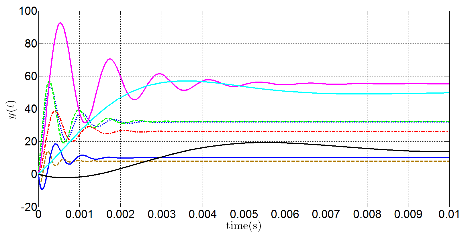
Figures 11 12 13 14 present some examples of the application of the $\mathcal{C}_{\pi}$ -control under different arbitrary switching sequences that involve both minimum and non-minimum phase systems. The first switching time is $t_{1}$ , the second is $t_{2}$ and the third is $t_{3}$ .

Consider now the existence of a delay $\tau$ on $y$ that modify (4) such that:

\Sigma_{p}(u\longmapsto y):=\left\{\begin{array}[]{l}\dot{x}(t)=A_{p}x(t)+B_{p}u(t)\\ y=C_{p}x(t-\tau)\end{array}\right.

(5)

This delay can e.g. simulate the propagation delay inside a sensor network. Figures 15 and 16 present two examples of the application of the $\mathcal{C}_{\pi}$ -control under different switching sequences that involve both minimum and non-minimum phase systems.

Discussions

These results have been obtained with a single specific set of the $\mathcal{C}_{\pi}$ -parameters; to improve the tracking performances, one may consider an on-line adjustment of the $\mathcal{C}_{\pi}$ -parameters. Although resonances occur at the instants of switches, the stability of the control is preserved (regarding the studied cases) when switching from the different types of systems. In the same manner, a direct tuning of the $\mathcal{C}_{\pi}$ -parameters could damp (ideally, could cancel) the resonant effects.

The presented simulation results show that the proposed control law is robust to ”strong” model variations and in particular when the model is a switching non-minimum phase or minimum phase system that include eventually time-delay. Moreover, the proposed control law seems to have the same properties than the original model-free control [2] [3] for which its performances have been successfully verified especially in simulation.

3.3 Ballistic and the fire control

If one fire a projectile at an initial angle and an initial speed, then general physics allows calculating how far it will travel… but would it be possible to control the initial speed needed in such manner that the projectile reaches a precise distance? That’s what we propose to do using the $\mathcal{C}_{\pi}$ -control.

3.3.1 Ballistic simplified model

We define first a simple model of the trajectory $\mathbf{w}(t)=(w_{x}(t),\,w_{z}(t))$ of a projectile of mass m in the usual frame of reference $(Oxz)$ fired with an initial speed magnitude ${v_{0}}$ that makes a fire angle $\theta$ with the horizontal reference i.e. $\mathbf{v}(t)=v_{0}\cos(\theta)\mathbf{e}_{x}+v_{0}\sin(\theta)\mathbf{e}_{z}$ . The origin $(0,0)$ of the frame reference is considered as the initial position of the projectile.

Denote $\mathbf{a}$ the acceleration vector and $\mathbf{v}$ the speed vector of the projectile. From Newton law, considering the action of the gravity $\mathbf{g}$ and the air resistance $c\mathbf{v}^{2}$ , we have:

m\frac{d^{2}\,\mathbf{w}(t)}{d\,t^{2}}=m\mathbf{a}=m\mathbf{g}-c\mathbf{v}^{2}

(6)

with the initial conditions:

\left.\frac{d\,w_{x}(t)}{d\,t}\right|_{(0,0)}=v_{0}\cos\theta,\qquad\left.\frac{d\,w_{z}(t)}{d\,t}\right|_{(0,0)}=v_{0}\sin\theta

(7)

Considering no air resistance i.e. $c=0$ , (6) is simplified:

\left\{\begin{array}[]{c}\displaystyle{m\frac{d\,w_{x}(t)}{d\,t}=0}\\ \\[0.28436pt] \displaystyle{m\frac{d\,w_{z}(t)}{d\,t}=-mg}\end{array}\right.

(8)

whose solution reads:

\left\{\begin{array}[]{c}\displaystyle{w_{x}(t)=v_{0}\cos\theta\,t+cte}\\ \\[0.28436pt] \displaystyle{w_{z}(t)=v_{0}\sin\theta\,t-\frac{1}{2}gt^{2}+cte}\end{array}\right.

(9)

From (9), the range (or the target) of the projectile $x_{d}$ at $z=0$ can be easily deduced. We have:

d=\frac{2v_{0}^{2}\cos\theta\sin\theta}{g}.

(10)

3.3.2 Ballistic-fire control methodology

Proposed strategy

Consider by hypothesis that a ”virtual” trajectory $\mathbf{w^{*}}$ of the projectile hits a target $x_{d}^{*}$ from an initial speed $v_{0}^{*}$ and an initial fire angle $\theta^{*}$ .

Consider now the ”true” projectile to fire with a trajectory $\mathbf{w}$ . To hit the target $x_{d}^{*}$ (at $z=0$ ) from a small initial speed $v_{\varepsilon}$ , one controls the projectile in such manner that the projectile reaches quickly the initial speed $v_{0}^{*}$ and the initial fire angle $\theta^{*}$ required to hit the specified target $x_{d}^{*}$ according to (10). During such ”launching” phase, that we define as the ”launching” distance $\Delta x_{0}$ for which the trajectory of the projectile is fully controlled, we start from an initial condition that prevents the projectile to reach its target $x_{d}^{*}$ i.e. :

\left.\frac{d\,w_{x}(t)}{d\,t}\right|_{(0,0)}=v_{\varepsilon}\cos\theta_{\varepsilon},\qquad\left.\frac{d\,w_{z}(t)}{d\,t}\right|_{(0,0)}=v_{\varepsilon}\sin\theta_{\varepsilon}

(11)

where $v_{\varepsilon}<v_{0}^{*}$ and $\theta_{\varepsilon}\leq\theta^{*}$ are positive resp. initial speed magnitude and fire angle. Figure 17 illustrates simulation examples of a ”virtual” trajectory (subj. to $v_{0}^{*}$ and $\theta^{*}$ ) and a ”true” trajectory (subj. to $v_{\varepsilon}$ and $\theta^{*}$ ) that is not controlled; the simulations of the trajectories considering $c\neq 0$ are presented in Fig. 17(b).

The goal is to accelerate the projectile using a specific mechanical device in such manner that the references $v_{0}^{*}$ and $\theta^{*}$ are reached quickly. We consider therefore controlling the trajectory $\mathbf{w}(t)$ of the projectile over the launching distance $\Delta x_{0}$ .

Controllable ballistic model

To simulate a controllable model of the trajectory $\mathbf{w}$ of the projectile, we consider adding an external acceleration force in (6) that represents the mechanical action of the specific mechanical device over the distance $\Delta x_{0}$ . We have:

m\frac{d^{2}\,\mathbf{w}(t)}{d\,t^{2}}=m\mathbf{g}-c\mathbf{v}^{2}+\mathbf{a}^{ext}

(12)

where $\mathbf{a}^{ext}(t)=(a^{ext}_{x}(t),\,a^{ext}_{z}(t))$ is equivalent to the external force provided by the mechanical device. Since such device acts only over $\Delta x_{0}$ , then we assume that $\mathbf{a}^{ext}=\mathbf{0}$ for all $x>\Delta x_{0}$ .

3.3.3 Implementation of the $\mathcal{C}_{\pi}$ -controller

A possible control scheme is to consider controlling the trajectory $\mathbf{w}$ that must be ”as close as possible” to the reference $\mathbf{w^{*}}$ over the distance $\Delta x_{0}$ . Therefore, $\mathbf{w}$ is physically measured and the external acceleration $\mathbf{a}^{ext}$ is driven by the $\mathcal{C}_{\pi}$ -controller, through the specific mechanical device.

We build a closed-loop that creates a feedback between (2) and (12). We have ”symbolically”, for all $x\leq\Delta x_{0}$ :

\left\{\begin{array}[]{c}\displaystyle{\mathbf{u}_{k}=\mathbf{a}^{ext}_{k}=\left.\int_{0}^{t}K_{i}(\mathbf{w}^{*}_{k-1}-\mathbf{w}_{k-1})d\,\tau\right|_{k-1}\underbrace{\left\{\mathbf{u}_{k-1}^{i}+{K_{p}}(\alpha e^{-\beta k}-\mathbf{w}_{k-1})\right\}}_{\mathbf{u}_{k}^{i}}}\\ \\[2.84544pt] \displaystyle{m\frac{d^{2}\,\mathbf{w}(t)}{d\,t^{2}}=m\mathbf{g}-c\mathbf{v}^{2}+\mathbf{u}_{k}}\end{array}\right.

(13)

Determination of the distance $\mathbf{\Delta x_{0}}^{*}$

Since we expect that the projectile is fired from $\Delta x_{0}$ with a speed that is very close to $v_{0}^{*}$ (and follows, via the $\mathcal{C}_{\pi}$ -control, the same trajectory i.e. $w\approx w^{*}$ over $\Delta x_{0}$ ), then, we propose a possible definition of the theoretical launching distance $\Delta x_{0}^{*}$ , (considered only over the $x$ axis) that corresponds to the solution in $w_{x}$ of:

\frac{d\,w_{x}(t)}{d\,t}=v_{0\,x}^{*}

(14)

Geometrically, the theoretical launching distance $\Delta x_{0}^{*}$ is associated to the speed $v_{x}$ that is reached by the projectile (launched with the initial speed $v_{\varepsilon}<v_{0}^{*}$ ) when $v_{x}$ is close to $v_{0\,x}^{*}$ .

3.3.4 Numerical simulations

Case $\mathbf{\Delta x_{0}}>\mathbf{\Delta x_{0}}^{*}$

Consider the simulated ”virtual” trajectory, presented in Fig. 17, as the control reference ${w^{*}}$ ; to simplify, we consider $\theta$ as constant. Figure 18 presents the case where the fire is controlled considering $c=0$ over $\Delta x_{0}=0.11$ m. In particular, Fig. 18(a) presents, at the top, the evolution of the controlled trajectory ${w}$ in comparison with the reference $w^{*}$ , and, at the bottom, the calculated speed $d\,{w_{x}}/d\,t$ in comparison with the initial speed $v_{0}\cos\theta$ . Figure 18(b) presents the complete ”true” controlled trajectory in comparison with the virtual trajectory. Figure 19 presents the same simulations in the case $c\neq 0$ .

Case $\mathbf{\Delta x_{0}}\sim\mathbf{\Delta x_{0}}^{*}$

Consider the simulated ”virtual” trajectory, presented in Fig. 17, as the control reference ${w^{*}}$ ; to simplify, we consider $\theta$ as constant. Figure 20 presents the case where the fire is controlled considering $c=0$ over $\Delta x_{0}^{*}$ . In particular, Fig. 20(a) presents, at the top, the evolution of the controlled trajectory ${w}$ in comparison with the reference $w^{*}$ , and, at the bottom, the calculated speed $d\,{w_{x}}/d\,t$ in comparison with the initial speed $v_{0}\cos\theta$ . Figure 20(b) presents the complete ”true” controlled trajectory in comparison with the virtual trajectory. Figure 21 presents the same simulations in the case $c\neq 0$ .

Discussions

These results have been obtained using the same set of the $\mathcal{C}_{\pi}$ -parameters. The properties of stabilization of the control law, like in the previous case when dealing with switching systems (§3.2) , seem to be preserved and ensure good tracking performances in particular when considering $c=0$ and $c\neq 0$ .

Further generalizations would allow using multiple and parallel $\mathcal{C}_{\pi}$ -controllers in order to control simultaneous physical quantities. In particular, the speed profile $\mathbf{v}$ could be controlled simultaneously with the trajectory $\mathbf{w}$ …

3.4 Control of the HIV-1 model

The problem is to control the predator-prey like model that describes the evolution of the HIV-1 when subjected to an external ”medical agent”. From a mathematical point of view, we study the possibility of controlling the model (15) for which the purpose is to control the output $y$ (corresponding to the viral load) using the double inputs $u_{1}$ and $u_{2}$ in such manner that $y$ converges rapidly to zero ⁸⁸ 8 Since we are trying to control this model only from the mathematical point of view, we do not take into account the constraints that are medically imposed. [16] [17].

\left\{\begin{array}[]{l}\dot{x}_{1}=s-dx_{1}-(1-u_{1})\beta x_{1}x_{3}\\ \dot{x}_{2}=(1-u_{1})\beta x_{1}x_{3}-\mu x_{2}\\ \dot{x}_{3}=(1-u_{2})kx_{2}-cx_{3}\\ y=\begin{pmatrix}0&0&\gamma\end{pmatrix}x\end{array}\right.

(15)

where (mathematically) : $d=0.02,k=100,s=10,\beta=2.4.10^{-5},\mu=0.24,c=2.4$ . $\gamma$ is a scaling factor that allows normalizing the output. Figure 22 presents the evolution of the output $y$ in open-loop when $u_{1}=u_{2}=0$ i.e. when no medical drug is considered. Figures 23 and 24 illustrate the control of $y$ considering two different ratios between $u_{1}$ and $u_{2}$ .

3.5 Control of the Epstein frame

The Epstein frame (see Fig. 25 ⁹⁹ 9 Picture taken from Wikipédia http://upload.wikimedia.org/wikipedia/commons/5/51/Epstein_frame.jpg.) aims to characterize a magnetic material by determining its $B-H$ hysteresis curve. The principle is to create a magnetic field $H$ inside the material using a ”magnetizing” current $i_{H}$ . The material gives a response to the field $H$ that physically corresponds to the measurable magnetic induction field $B$ . This $B$ field creates a voltage $v_{B}$ through magnetic induction and the quantities $v_{B}$ and $i_{H}$ is a representation of the magnetic hysteresis curve $B-H$ . To describe experimentally the major $B-H$ hysteresis loop, the material under study has to be magnetized using a current $i_{H}$ that is alternative and of enough magnitude in order to describe the magnetic behavior at saturation. The purpose of the control law implementation is to control $i_{H}$ such that the output voltage of the Epstein frame $v_{B}$ remains ”as close as possible” to a desired reference waveform.

3.5.1 Epstein frame control

Proposed $\mathcal{C}_{\pi}$ -control scheme

Consider the control scheme depicted in Fig. 26 where $\mathcal{C}_{\pi}$ is the proposed PMA controller. $K_{in}$ and $K_{out}$ are positive real gains. Denote $f_{BH}$ the numerical Jiles-Atherton model that is associated to the magnetic hysteresis $B-H$ and $f_{JA}$ is the complete hysteresis to control.

Jiles-Atherton based hysteresis model

The Jiles-Atherton model [18] describes a magnetic hysteresis cycle $B-H$ . It reads:

\frac{d\,M}{d\,H}=\frac{1}{1+c}\frac{M_{an}-M}{\delta k-\alpha(M_{an}-M)}+\frac{c}{1+c}\frac{d\,M_{an}}{d\,H}

(16)

where $c$ , $\delta k$ , $M_{an}$ , $\alpha$ are physical coefficients well identified from magnetic hysteresis measurement and we assume that the current $i_{H}$ corresponds to the magnetization $H$ i.e. $i_{H}\propto H$ and the voltage $v_{B}$ corresponds to the derivative of the magnetic induction field response $B=\mu_{0}H+J_{BH}(H)$ (where $J_{BH}$ describes the $B-H$ hysteresis via (16)).

Simplified model of the Epstein frame

The Epstein frame admits a complex model based on the Jiles-Atherton model that represents all electric phenomena that occur inside the Epstein frame¹⁰¹⁰ 10 The Epstein frame is equivalent to a transformer and the ”mutual interactions” between primary and secondary coils must be taken into account in addition to the hysteresis behavior.. To simplify the model of the Epstein frame to control, we consider controlling a nonlinear function $f_{JA}$ , which represents a modified Jiles-Atherton model. Denote $v_{H}=f_{JA}(i_{H})$ the nonlinear dynamical system that describes the $B-H$ hysteresis as a function of $i_{H}$ , and consider controlling directly the hysteresis cycle in such manner that $\mathcal{C}_{\pi}$ controls $i_{H}$ in order to get $v_{H}=f_{JA}(i_{H})$ as close as possible to a reference waveform.

To define the global $f_{JA}$ hysteresis function that is controlled by $\mathcal{C}_{\pi}$ , which includes the scaling coefficients needed by the $\mathcal{C}_{\pi}$ corrector, consider $i_{H}=K_{in}\,u$ , $y=K_{out}v_{H}$ and a coefficient $K_{e}$ such that:

y=f_{JA}(u)=K_{in}K_{e}u+K_{out}J_{BH}(K_{in}u).

(17)

The small coefficient $K_{e}\,\#\,10^{-4}$ compensates the very small variations of $f_{BH}$ when $B$ is close to $B_{sat}$ . Such variations may induce time-delays in the response of the $\mathcal{C}_{\pi}$ -controller that induce some distortions of the output signal $y$ . The model (17) could be seen as an ”affine” derivation of the original Jiles-Atherton model.

The $B-H$ loops, obtained from the Jiles-Atherton model, are depicted in Fig. 27 considering the frequencies 5 Hz, 50 Hz, 500 Hz, 1 kHz and 10 kHz. Since this hysteresis model does not allow $H>H_{max}$ , a limitation is necessary to bound the evolution of $H$ , that may occur eventually during the transient of the dynamic stabilization of the control loop (ex. in Fig. 31).

3.5.2 Simulation results

Figures 28, 29, 30, 31 and 32 depict the input $u$ and the (rescaled) output $y$ of the control loop according to the time. Given a particular operating frequency, for which a particular $H-B$ hysteresis is studied (see Fig. 27), and assuming that the output reference $y^{*}$ is a sinusoid, whose magnitude corresponds to the theoretical $H_{max}$ of the $H-B$ hysteresis, different frequencies are considered (5 Hz, 50 Hz, 500 Hz, 1 kHz and 10 kHz) in order to highlight the behavior of the controlled voltage $v_{b}$ when the frequency changes. In particular, high frequencies (e.g. Figures 31 and 32) introduce an important transient response on $y$ due to the fact that the variations of $y^{*}$ are too fast to get an immediate stabilization to the dynamic working point of the hysteresis. The simulation show that the $\mathcal{C}_{\pi}$ -controller gives very interesting dynamic performances over a wide range of dynamic working points relating to the operating frequency. An optimization algorithm (see §2.3) has been used to adjust the parameters of the $\mathcal{C}_{\pi}$ -controller in such manner that the shape of the output response $y$ is ”as close to” a sine shape¹¹¹¹ 11 Remember that the purpose of the optimization procedure is to minimize the tracking error $y^{*}-y$ in such manner that ideally $y\equiv y^{*}$ for the particular sine output reference $y^{*}$ ..

Remarks

This hysteresis model is composed of three subsystems (the first magnetization branch, the increasing and decreasing branches) that switch depending on the value of $dH/dt$ . When $H<<H_{max}$ , the switch between the branches may not be smooth and such ”connection” may induce a small transient on $y$ . An illustration is presented in Fig. 33 at a low frequency in comparison with Fig. 30.

The closed-loop has been also tested using a triangular shaped output reference $y^{*}$ . Figure 34 depicts the magnitude of the magnetic field $H$ and the corresponding (rescaled) magnetic induction $B$ during the control loop process according to the time. The frequency of 5 Hz has been considered as an example holding the parameters of the simulation with the sine reference at 5 Hz.

4 Derivative-free $\&$ ”extremum-seeking” control

To describe how the PMA could be used as a derivative-free optimization (DFO) algorithm (e.g. [19] [20]) or as an ”extremum-seeking” (ES) control scheme (e.g. [21] [22] [23]), we first define each element of the associated control scheme and then, we derive the operating conditions that would allow to minimize nonlinear functions. We assume that it is possible to derive a control scheme such that the PMA can be used to minimize nonlinear functions.

4.1 Proposed $\mathcal{C}_{\pi}$ -control scheme

Definition of the closed loop

Consider the control scheme depicted in Fig. 35 where $\mathcal{C}_{\pi}$ is the proposed PMA ”extremum-seeking” controller. $K_{in}$ and $K_{out}$ are positive real gains. We consider either a static nonlinear function $f_{nl}^{s}$ (regarding DFO), which does not have any internal dynamical properties, or a nonlinear SISO dynamical system (1) (regarding ES), to minimize. The function $Q$ is e.g. a basic first order transfer function.

Function to control

•

Define the $f_{nl}^{s}$ static function to optimize such that:

$f_{nl}^{s}:\begin{array}[]{c}\mathbb{R}^{n}\rightarrow\mathbb{R}\\ u^{\prime}\mapsto y\end{array}$ (18)

or consider a nonlinear SISO dynamical system (1).

This function represents the ”nonlinear optimization problem”. Currently, the assumption $n\leq 2$ is considered and we denote $u^{\prime}_{x}$ the input variable for $n=1$ .

•

$Q$ is a standard linear transfer function (typically of first order), such that:

Q:\begin{array}[]{c}\mathbb{R}\rightarrow\mathbb{R}\\ \displaystyle{\left.\frac{du^{\prime}}{dt}\right|_{k}+\gamma\left.u^{\prime}\right|_{k}=u_{k}}\end{array}

(19)

where $\gamma$ is a time-constant, chosen in such manner that the step response of $Q$ is very fast. As presented in the Fig. 35, $Q$ is associated with $f_{nl}^{s}$ in order to provide some minimal dynamical properties regarding the system $f_{nl}^{s}$ to control. Obviously, the $Q$ function is not necessary when $f_{nl}$ is already a dynamical function like (1)¹²¹² 12 Last investigations suggest that the linear transfer function $Q$ may be not necessary even for a $f_{nl}^{s}$ function to control. The properties of the para-model algorithm are currently under study considering nonlinear systems that are ”non-dynamical”..

A single $\mathcal{C}_{\pi}$ -controller¹³¹³ 13 To extend this scheme to multi-input variables $(n>2)$ of $f_{nl}$ , one may consider the use of a $\mathcal{C}_{\pi}$ -controller per input variable. drives a single input of $f_{nl}$ (eventually through $Q$ ), as presented in Fig. 35.

4.2 Numerical applications

Since the PMA is designed for nonlinear systems and does not contain any derivatives, it is assumed that the ”extremum-seeking” control is possible considering a specific definition of $y^{*}$ in order to reach and stabilize $f_{nl}$ to its minimum.

Let us assume that the following (eventually constrained) minimization problem (described for a single variable):

\min_{x\in\mathbb{R}}\,f_{nl}(x),\quad(x=u^{\prime}\,\hbox{identically inside the control scheme})

(20)

is equivalent to the control scheme described in Fig. 35, for which the output reference $y^{*}$ ”follows” the minimum value of $f_{nl}$ . We denote $x=x_{opt}$ the value that gives the minimum of $f_{nl}$ .

Results

For each case in 1D, are plotted: the difference between two iterations $y_{k},\,y_{k-1}$ and the error between $x_{opt}$ and the evolution of $x$ through the closed-loop. In these cases, all the parameters of $\mathcal{C}_{\pi}$ have been set experimentally to give interesting performances but are not optimal (the choice of the $y^{*}$ function may influence the speed of the convergence). The following numerical cases are studied:

•

See Fig. 36 regarding the minimization of a 1D convex function such that:

$\min_{x}\,(x-30)^{2}$ (21)
•

See Fig. 37 regarding the minimization of a 1D convex function with a minimum that changes according to the time at an unknown instant $t_{1}$ such that:

$\min_{x}\,(x-30)^{2}\stackrel{{\scriptstyle t_{1}\,?}}{{\rightarrow}}\min_{x}(x-40)^{2}$ (22)
•

See Fig. 38 regarding the minimization of a 1D non convex function such that:

$\min_{x,y}\,10(1.5\cos(x)-x)+\exp(x-5)+100\quad\hbox{subj. to :}\quad y\geq 15x-60$ (23)

5 Concluding remarks

We presented how the proposed para-model agent¹⁴¹⁴ 14 Why ”para-model”? Based on the ”model-free” methodology, for which the model is not correlated to the controller in the sense that the controller does not need an explicit definition of the model to be parametrized and can thus rebuild an ultra-local model from measurements, we propose the prefix ”para” to highlight the fact that the agent is ”in close proximity” to the model of the process that he controls. Although no specific information is needed for the PMA control part, some basic information may be needed to configure properly the PMA and the output reference $y^{*}$ in the case of extremum-seeking control approach. The stability study is an essential part that should formalize the proposed PMA approach in order to justify theoretically the operating conditions of the $\mathcal{C}_{\pi}$ -control., as a model-free and derivative-free based controller, can be used to control nonlinear systems or perform optimization / ”extremum-seeking” control. Further investigations include extensive tests and applications to complex systems as well as a complete study of the stability.

Acknowledgement

The author is sincerely grateful to Dr. Edouard Thomas for his strong guidance and his valuable comments that improved this paper. The author is also sincerely grateful to Olivier Ghibaudo, Ph.D. student at G2Elab-CNRS (Grenoble) France, for having worked on the numerical version of the hysteresis model.

References

[1] M. Fliess, C. Join, M. Mboup and H. Sira-Ramirez, ”Vers une commande multivariable sans modèle”, Conférence internationale francophone d’automatique (CIFA 2006), France, 2006. (available in french at https://arxiv.org/pdf/math/0603155.pdf).
[2] M. Fliess and C. Join, ”Commande sans modèle et commande à modèle restreint”, e-STA, vol. 5 (n^∘ 4), pp. 1-23, 2008 (available at http://hal.inria.fr/inria-00288107/en/).
[3] M. Fliess and C. Join, ”Model-free control”, International Journal of Control, vol. 86, issue 12, pp. 2228-2252, Jul. 2013 (available at http://arxiv.org/pdf/1305.7085.pdf).
[4] K.J. Åström and P.R. Kumar, ”Control: A perspective”, Automatica, vol. 50, issue 1, pp. 3-43, Jan. 2014 (available at http://www.sciencedirect.com/science/article/pii/S0005109813005037).
[5] K. J. Åström, ”Direct methods for nonminimum phase systems”, in 19th IEEE Conference on Decision and Control including the Symposium on Adaptive Processes, vol.19, pp.611-615, Dec. 1980.
[6] A. Isidori, ”A tool for semi-global stabilization of uncertain non-minimum-phase nonlinear systems via output feedback”, IEEE Transactions on Automatic Control, vol.45, no.10, pp. 1817-1827, Oct. 2000.
[7] N. Wang, W. Xu and F. Chen, ”Adaptive global output feedback stabilisation of some non-minimum phase nonlinear uncertain systems”, IET Control Theory & Applications, vol.2, no.2, pp.117-125, Feb. 2008.
[8] M. Benosman, F. Liao, K.-Y. Lum and J. Liang Wang, ”Nonlinear Control Allocation for Non-Minimum Phase Systems”, IEEE Transactions on Control Systems Technology, vol.17, no.2, pp.394-404, Mar. 2009.
[9] R. Gurumoorthy and S.R. Sanders, ”Controlling Non-Minimum Phase Nonlinear Systems - The Inverted Pendulum on a Cart Example”, 1993 American Control Conference, pp.680-685, June 1993.
[10] D. Karagiannis, Z.P. Jiang, R. Ortega and A. Astolfi, ”Output-feedback stabilization of a class of uncertain non-minimum-phase nonlinear systems”, Automatica, vol. 41, Issue 9, September 2005.
[11] I. Barkana, ”Classical and simple adaptive control for nonminimum phase autopilot design”, Journal of Guidance Control and Dynamics, vol. 28, Issue: 4, pp. 631-638, 2005.
[12] L. Michel, C. Join, M. Fliess, P. Sicard and A. Chériti, ”Model-free control of dc/dc converter”, in 2010 IEEE 12th Workshop on Control and Modeling for Power Electronics, pp.1-8, June 2010 (available at http://hal.inria.fr/inria-00495776/).
[13] L. Michel, ”Model-free control of non-minimum phase systems and switched systems”, preprint arXiv, 2011 (available at http://arxiv.org/abs/1106.1697).
[14] M. Porcelli and Ph. L. Toint, BFO, ”A trainable derivative-free Brute Force Optimizer for nonlinear bound-constrained optimization and equilibrium computations with continuous and discrete variables”, Namur Center for Complex Systems, In Support, Tech. Reports, no. naXys-06-2015, Belgium, Jul. 2015 (available at http://www.optimization-online.org/DB_FILE/2015/07/4986.pdf).
[15] F. Cannavó, ”Sensitivity analysis for volcanic source modeling quality assessment and model selection”, Computers $\&$ Geosciences, vol. 44, pp. 52-59, Jul. 2012.
[16] M. Barão and J.M. Lemos, ”Nonlinear control of HIV-1 infection with a singular perturbation model”, Biomedical Signal Processing and Control, vol. 2, issue 3, pp. 248-257, Jul. 2007.
[17] I. K. Craig, X. Xia and J. W. Venter, ”Introducing HIV/AIDS education into the electrical engineering curriculum at the University of Pretoria,” IEEE Transactions on Education, vol. 47, no. 1, pp. 65-73, Feb. 2004.
[18] D. C. Jiles and D. L. Atherton, ”Theory of ferromagnetic hysteresis”, J. Appl. Phys. 55, 2115 (1984).
[19] A.R. Conn, K. Scheinberg and L.N. Vicente, ”Introduction to Derivative-Free Optimization”, SIAM Publications (Philadelphia), 2009.
[20] L. M. Rios and N. V. Sahinidis, ”Derivative-free optimization: a review of algorithms and comparison of software implementations”, Journal of Global Optimization, Volume 56, Issue 3, pp 1247-1293, Jul. 2013 (available at http://link.springer.com/article/10.1007/s10898-012-9951-y).
[21] K. B. Ariyur and M. Krstic, ”Real-Time Optimization by Extremum-Seeking Control”, Wiley, 2003.
[22] Y. Tan, W.H. Moase, C. Manzie, D. Nesic and I.M.Y. Mareels, ”Extremum Seeking From 1922 To 2010”, 2010 29th Chinese Control Conference (CCC), pp.14,26, 29-31 Jul. 2010.
[23] A. O. Vweza, K. To Chong and D. J. Lee, ”Gradient-free numerical optimization-based extremum seeking control for multiagent systems”, International Journal of Control, Automation and Systems, May 2015.

1 Introduction

2 General Principle

2.1 Definition of the closed-loop

2.2 Definition of the PMA algorithm

Practical algorithm

Remark

2.3 Performances in simulation

2.3.1 Optimization of the closed-loop

2.3.2 Sobol-based sensibility of the controlled transient

3 Applications of the 𝒞π\mathcal{C}_{\pi}-control

3.1 Motor control in the d​qdq frame

3.2 Control of switched non-minimum and minimum phase systems

Discussions

3.3 Ballistic and the fire control

3.3.1 Ballistic simplified model

3.3.2 Ballistic-fire control methodology

Proposed strategy

Controllable ballistic model

3.3.3 Implementation of the 𝒞π\mathcal{C}_{\pi}-controller

Determination of the distance 𝚫​𝐱𝟎∗\mathbf{\Delta x_{0}}^{*}

3.3.4 Numerical simulations

Case 𝚫​𝐱𝟎>𝚫​𝐱𝟎∗\mathbf{\Delta x_{0}}>\mathbf{\Delta x_{0}}^{*}

Case 𝚫​𝐱𝟎∼𝚫​𝐱𝟎∗\mathbf{\Delta x_{0}}\sim\mathbf{\Delta x_{0}}^{*}

Discussions

3.4 Control of the HIV-1 model

3.5 Control of the Epstein frame

3.5.1 Epstein frame control

Proposed 𝒞π\mathcal{C}_{\pi}-control scheme

Jiles-Atherton based hysteresis model

Simplified model of the Epstein frame

3.5.2 Simulation results

Remarks

4 Derivative-free &\& ”extremum-seeking” control

4.1 Proposed 𝒞π\mathcal{C}_{\pi}-control scheme

Definition of the closed loop

Function to control

4.2 Numerical applications

Results

5 Concluding remarks

Acknowledgement

References

3 Applications of the $\mathcal{C}_{\pi}$ -control

3.1 Motor control in the $dq$ frame

3.3.3 Implementation of the $\mathcal{C}_{\pi}$ -controller

Determination of the distance $\mathbf{\Delta x_{0}}^{*}$

Case $\mathbf{\Delta x_{0}}>\mathbf{\Delta x_{0}}^{*}$

Case $\mathbf{\Delta x_{0}}\sim\mathbf{\Delta x_{0}}^{*}$

Proposed $\mathcal{C}_{\pi}$ -control scheme

4 Derivative-free $\&$ ”extremum-seeking” control

4.1 Proposed $\mathcal{C}_{\pi}$ -control scheme