跳到论文正文
W Papers独立论文阅读器 arXiv:1202.4641 论文正文 计算阅读时间 · 0%
引用这篇论文根据当前论文元数据生成,正式投稿前建议核对。


License: arXiv.org perpetual non-exclusive license
arXiv:1202.4641v1 [math.NT] 21 Feb 2012

Computation of Polarized Metrized Graph Invariants By Using Discrete Laplacian Matrix

Zubeyir Cinkir Address: Zubeyir Cinkir
Department of Mathematics
Zirve University
27260, Gaziantep, TURKEY
Email address: zubeyir.cinkir@zirve.edu.tr
Abstract.

Several invariants of polarized metrized graphs and their applications in Arithmetic Geometry are studied recently. In this paper, we give fast algorithms to compute these invariants by expressing them in terms of the discrete Laplacian matrix and its pseudo inverse. Algorithms we give can be used for both symbolic and numerical computations. We present various examples to illustrate the implementation of these algorithms.

Key words and phrases: 
Metrized graph, polarized metrized graph, invariants of polarized metrized graphs, the tau constant, resistance function, the discrete Laplacian matrix, pseudo inverse and relative dualizing sheaf

1. Introduction

Let XX be a geometrically connected curve of genus g¯≥2\bar{g}\geq 2 over a field kk. Suppose kk is either a number field or the function field of a smooth projective curve YY over a field. Assume that XX has a semistable model 𝒳{\mathcal{X}} over 𝒮{\mathcal{S}}, where 𝒮=S​p​e​c​𝒪k{\mathcal{S}}=Spec\mathcal{O}_{k} if kk is a number field and 𝒮=Y{\mathcal{S}}=Y if kk is a function field. Let N⁡(v)N(v) be the local factor related to the product formula for kk. In this context, ω𝒳/𝒮2\omega_{{\mathcal{X}}/{\mathcal{S}}}^{2}, the self intersection of the relative dualizing sheaf ω𝒳/𝒮\omega_{{\mathcal{X}}/{\mathcal{S}}}, is an important quantity both in geometric and arithmetic case. Lower and upper bounds to this quantity are of interest in diophantine geometry.

In 1993, Zhang [24] expressed ω𝒳/𝒮2\omega_{{\mathcal{X}}/{\mathcal{S}}}^{2} in terms of ωa2\omega_{a}^{2}, the self intersection of the admissible relative dualizing sheaf ωa\omega_{a} associated to a minimal regular model of XX:

(1) ω𝒳/𝒮2=ωa2+∑vϵ⁡(Xv)​log⁡N⁡(v),\begin{split}\omega_{{\mathcal{X}}/{\mathcal{S}}}^{2}=\omega_{a}^{2}+\sum_{v}\epsilon(X_{v})\log N(v),\end{split}

where vv runs over the set of non-archimedean places of kk, and ϵ⁡(Xv)\epsilon(X_{v}) is a certain local invariant of the reduction graph R⁡(Xv)R(X_{v}) associated to the completion of XX at a place vv of kk.

In 2010, Zhang [25, Corollary 1.3.2] expressed ωa2\omega_{a}^{2} in terms of ⟨Δξ,Δξ⟩\langle\Delta_{\xi},\Delta_{\xi}\rangle, the arithmetic self intersection (equal to the canonical height) of the Gross-Schoen cycle Δξ⊂X×X×X\Delta_{\xi}\subset X\times X\times X:

(2) ωa2=2​g¯−22​g¯+1​⟨Δξ,Δξ⟩+2​g¯−22​g¯+1​∑vφ⁡(Xv)​log⁡N⁡(v),\begin{split}\omega_{a}^{2}=\frac{2\bar{g}-2}{2\bar{g}+1}\langle\Delta_{\xi},\Delta_{\xi}\rangle+\frac{2\bar{g}-2}{2\bar{g}+1}\sum_{v}\varphi(X_{v})\log N(v),\end{split}

where vv runs over the set of places of kk, and φ⁡(Xv)\varphi(X_{v}) is a certain local invariant again linked to the reduction graph R⁡(Xv)R(X_{v}) at each place vv of kk.

On the other hand, we have the following equality for a semistable fibration f:𝒳⟶𝒮f:{\mathcal{X}}\longrightarrow{\mathcal{S}} by Nother’s formula:

(3) ω𝒳/𝒮2=12​deg⁡f∗​(ω𝒳/𝒮)−∑vδ⁡(Xv),\begin{split}\omega_{{\mathcal{X}}/{\mathcal{S}}}^{2}=12\deg f_{*}(\omega_{{\mathcal{X}}/{\mathcal{S}}})-\sum_{v}\delta(X_{v}),\end{split}

where δ⁡(Xv)\delta(X_{v}) is the total number of the singular points in the fiber over vv. Moreover, Zhang [25] showed that

(4) deg⁡f∗​(ω𝒳/𝒮)=g¯−16​(2​g¯+1)​⟨Δξ,Δξ⟩+∑vλ⁡(Xv)​log⁡N⁡(v),\begin{split}\deg f_{*}(\omega_{{\mathcal{X}}/{\mathcal{S}}})=\frac{\bar{g}-1}{6(2\bar{g}+1)}\langle\Delta_{\xi},\Delta_{\xi}\rangle+\sum_{v}\lambda(X_{v})\log N(v),\end{split}

where vv runs over the set of places of kk, and λ⁡(Xv)\lambda(X_{v}) is another local invariant associated to the reduction graphs R⁡(Xv)R(X_{v}). We refer [14] for other connections between λ⁡(Xv)\lambda(X_{v}) and some invariants of complex moduli space of curves of genus higher than 11.

Whenever vv is a non-archimedean place, the local invariants φ⁡(Xv)\varphi(X_{v}), ϵ⁡(Xv)\epsilon(X_{v}), λ⁡(Xv)\lambda(X_{v}) are defined as the invariants of the corresponding polarized metrized graph. Note that the reduction graph R⁡(X)R(X) of any semistable curve XX of genus g¯\bar{g} over a discrete valuation ring is a polarized metrized graph of genus g¯\bar{g}.

We also have invariants Z⁡(Γ)Z(\Gamma), τ⁡(Γ)\tau(\Gamma) and θ⁡(Γ)\theta(\Gamma) (see §2 below) of a polarized metrized graph Γ\Gamma, which are closely related to the local invariants given above.

Explicit computations of these local invariants were done only for some curves of genus less than or equal to 44 (see [17], [18], [11], [21], [22], [23], [13], [5]). Other than some families of polarized metrized graph of certain types, explicit computations become a huge intricate task for a person as soon as g¯\bar{g} gets larger than 3. Thus, one needs a computer algorithm to do such computations. We have such an algorithm to compute τ⁡(Γ)\tau(\Gamma) (see [5] and [9]). Also, X. Faber gave an algorithm to compute the invariants ϵ⁡(Γ)\epsilon(\Gamma), φ⁡(Γ)\varphi(\Gamma), λ⁡(Γ)\lambda(\Gamma) and Z⁡(Γ)Z(\Gamma) (see [11] and [12]).

In this paper, we provide a fast computer algorithm that can be used for both symbolic and numeric computation of each of the polarized metrized graph invariants. This algorithm is faster, because it takes advantage of two important facts: All of the effective resistance computations can be handled by just one matrix inversion (see Equation (11) and Lemma 3.2), and the computations of the invariants ϵ⁡(Γ)\epsilon(\Gamma), φ⁡(Γ)\varphi(\Gamma), λ⁡(Γ)\lambda(\Gamma) and Z⁡(Γ)Z(\Gamma) can be reduced to the computations of τ⁡(Γ)\tau(\Gamma) and θ⁡(Γ)\theta(\Gamma) (see Theorem 2.3).

In §2, we give a short revision of a polarized metrized graph and definitions of its invariants (see Lemma 2.1, Equation (8) and Equation (9)). Using Theorem 2.3, the problem of computing the invariants ϵ⁡(Γ)\epsilon(\Gamma), φ⁡(Γ)\varphi(\Gamma), λ⁡(Γ)\lambda(\Gamma) and Z⁡(Γ)Z(\Gamma) are reduced to the computations of τ⁡(Γ)\tau(\Gamma) and θ⁡(Γ)\theta(\Gamma). Using these connections and our previous results about τ⁡(Γ)\tau(\Gamma) and θ⁡(Γ)\theta(\Gamma), we explain how to deal with self loops and multiple edges, if desired, as the initial step of the algorithm.

In §3, we define discrete Laplacian matrices associated to polarized metrized graphs. We express θ⁡(Γ)\theta(\Gamma) in terms of the discrete Laplacian matrix L\mathrm{L} and its pseudo inverse L+\mathrm{L^{+}} (see Theorem 3.6). Then we use our previous result on τ⁡(Γ)\tau(\Gamma) to express the invariants ϵ⁡(Γ)\epsilon(\Gamma), φ⁡(Γ)\varphi(\Gamma), λ⁡(Γ)\lambda(\Gamma) and Z⁡(Γ)Z(\Gamma) in terms of the entries of L\mathrm{L} and L+\mathrm{L^{+}}. This gives us the main result in this paper. Namely, each of these invariants can be symbolically or numerically computed with the algorithm we provide.

Finally, we give various examples to show the implementation of our algorithm in §4.

2. Polarized Metrized graphs and their invariants

In this section, we first give brief descriptions of a metrized graph Γ\Gamma, a polarized metrized graph (Γ,q)(\Gamma,\textbf{q}), invariants τ⁡(Γ)\tau(\Gamma), θ⁡(Γ)\theta(\Gamma), ϵ⁡(Γ)\epsilon(\Gamma), φ⁡(Γ)\varphi(\Gamma), λ⁡(Γ)\lambda(\Gamma) and Z⁡(Γ)Z(\Gamma) associated to (Γ,q)(\Gamma,\textbf{q}).

A metrized graph Γ\Gamma is a finite connected graph equipped with a distinguished parametrization of each of its edges. A metrized graph Γ\Gamma can have multiple edges and self-loops. For any given p∈Γp\in\Gamma, the number υ⁡(p)\upsilon(p) of directions emanating from pp will be called the valence of pp. By definition, there can be only finitely many p∈Γp\in\Gamma with υ⁡(p)≠2\upsilon(p)\not=2.

For a metrized graph Γ\Gamma, we will denote a vertex set for Γ\Gamma by V⁡(Γ)V(\Gamma). We require that V⁡(Γ)V(\Gamma) be finite and non-empty and that p∈V⁡(Γ)p\in V(\Gamma) for each p∈Γp\in\Gamma if υ⁡(p)≠2\upsilon(p)\not=2. For a given metrized graph Γ\Gamma, it is possible to enlarge the vertex set V⁡(Γ)V(\Gamma) by considering additional valence 22 points as vertices.

For a given metrized graph Γ\Gamma with vertex set V⁡(Γ)V(\Gamma), the set of edges of Γ\Gamma is the set of closed line segments with end points in V⁡(Γ)V(\Gamma). We will denote the set of edges of Γ\Gamma by E⁡(Γ)E(\Gamma). However, if eie_{i} is an edge, by Γ−ei\Gamma-e_{i} we mean the graph obtained by deleting the interior of eie_{i}.

We define the genus of Γ\Gamma to be the first Betti number g⁡(Γ):=e−v+1g(\Gamma):=e-v+1 of the graph Γ\Gamma, where ee and vv are the number of edges and vertices of Γ\Gamma, respectively.

We denote the length of an edge ei∈E⁡(Γ)e_{i}\in E(\Gamma) by LiL_{i}, which represents a positive real number. The total length of Γ\Gamma, which is denoted by ℓ⁡(Γ)\ell(\Gamma), is given by ℓ⁡(Γ)=∑i=1eLi\ell(\Gamma)=\sum_{i=1}^{e}L_{i}.

If a metrized graph Γ\Gamma is viewed as a resistive electric circuit with terminals at xx and yy, with the resistance in each edge given by its length, then r⁡(x,y)r(x,y) is the effective resistance between xx and yy when unit current enters at yy and exits at xx.

For any xx, yy in Γ\Gamma, the resistance function r⁡(x,y)r(x,y) on Γ\Gamma is a symmetric function in xx and yy, and it satisfies r⁡(x,x)=0r(x,x)=0. For each vertex set V⁡(Γ)V(\Gamma), r⁡(x,y)r(x,y) is continuous on Γ\Gamma as a function of two variables and r⁡(x,y)≥0r(x,y)\geq 0 for all xx, yy in Γ\Gamma. For proofs of these facts and connections between the resistance function and the voltage function on Γ\Gamma, see articles [10], [2, sec 1.5 and sec 6], and [24, Appendix]. The resistance function r⁡(x,y)r(x,y) on a metrized graph were also studied in the articles [1] and [6].

We will denote by Ri​(Γ)R_{i}(\Gamma), or by RiR_{i} if there is no danger of confusion, the resistance between the end points of an edge eie_{i} of a graph Γ\Gamma when the interior of the edge eie_{i} is deleted from Γ\Gamma.

The tau constant τ⁡(Γ)\tau(\Gamma) of a metrized graph Γ\Gamma was initially defined by Baker and Rumely [2, Section 14]. The following lemma gives a description of the tau constant. In particular, it implies that the tau constant is positive.

Lemma 2.1.

[2, Lemma 14.4] For any fixed yy in Γ\Gamma, τ⁡(Γ)=14​∫Γ(∂∂x​r​(x,y))2​𝑑x\tau(\Gamma)=\frac{1}{4}\int_{\Gamma}\big(\frac{\partial}{\partial x}r(x,y)\big)^{2}dx.

One can find more detailed information on τ⁡(Γ)\tau(\Gamma) in articles [5], [6], [7] and [9].

On a metrized graph Γ\Gamma, we have a canonical measure μcan\mu_{\mathop{\rm can}} first studied by Chinburg and Rumely [10]. See the articles [2] and [6] for several interpretations of μc​a​n\mu_{can}. The following theorem gives an explicit description of μc​a​n\mu_{can}:

Theorem 2.2.

[10, Theorem 2.11] For a given metrized graph Γ\Gamma, let LiL_{i} and RiR_{i} be defined as before. Then we have

μcan​(x)=∑p∈V⁡(Γ)(1−12​v​(p))​δp​(x)+∑ei∈E⁡(Γ)d​xLi+Ri.\mu_{\mathop{\rm can}}(x)\ =\ \sum_{p\in V(\Gamma)}(1-\frac{1}{2}\text{v}\hskip 1.42262pt(p))\,\delta_{p}(x)+\sum_{e_{i}\in E(\Gamma)}\frac{dx}{L_{i}+R_{i}}.

Let Γ\Gamma be a metrized graph and let q:Γ→ℕ\textbf{q}:\Gamma\rightarrow{\mathbb{N}} be a function supported on the set of vertices of Γ\Gamma. The canonical divisor KK of (Γ,q)(\Gamma,\textbf{q}) is defined to be the following divisor on Γ\Gamma:

(5) K=∑p∈V⁡(Γ)(υ⁡(p)−2+2​q​(p))​p,andδK​(x)=∑p∈V⁡(Γ)(υ⁡(p)−2+2​q​(p))​δp​(x).\begin{split}K=\sum_{p\in V(\Gamma)}(\upsilon(p)-2+2\textbf{q}(p))p,\quad\text{and}\quad\delta_{K}(x)=\sum_{p\in V(\Gamma)}(\upsilon(p)-2+2\textbf{q}(p))\delta_{p}(x).\end{split}

The pair (Γ,q)(\Gamma,\textbf{q}) is called a polarized metrized graph (pm-graph in short) if q is non-negative and KK is an effective divisor. Whenever q=0\textbf{q}=0, (Γ,q)(\Gamma,\textbf{q}) is called a simple pm-graph. The genus g¯​(Γ)\bar{g}(\Gamma) of a pm-graph (Γ,q)(\Gamma,\textbf{q}) is defined to be

(6) g¯​(Γ)=1+12​deg⁡K=g⁡(Γ)+∑p∈V⁡(Γ)q​(p).\begin{split}\bar{g}(\Gamma)=1+\frac{1}{2}\deg{K}=g(\Gamma)+\sum_{p\in V(\Gamma)}\textbf{q}(p).\end{split}

We will simply use g¯\bar{g} instead of g¯​(Γ)\bar{g}(\Gamma) when there is no danger of confusion.

Let μa​d​(x)\mu_{ad}(x) be the admissible measure associated to KK (defined by Zhang [24, Lemma 3.7]). We have

μa​d​(x)=1g¯​(∑p∈V⁡(Γ)q​(p)​δp​(x)+∑ei∈E⁡(Γ)d​xLi+Ri).\mu_{ad}(x)=\frac{1}{\bar{g}}\Big(\sum_{p\in V(\Gamma)}\textbf{q}(p)\delta_{p}(x)+\sum_{e_{i}\in E(\Gamma)}\frac{dx}{L_{i}+R_{i}}\Big).

Then, if we use Theorem 2.2, we can relate μa​d​(x)\mu_{ad}(x) and μc​a​n​(x)\mu_{can}(x) as follows:

(7) μa​d​(x)=12​g¯​(2​μc​a​n​(x)+δK​(x)).\begin{split}\mu_{ad}(x)=\frac{1}{2\bar{g}}(2\mu_{can}(x)+\delta_{K}(x)).\end{split}

Moreover, δK​(Γ)=deg⁡(K)=2​g¯−2\delta_{K}(\Gamma)=\deg(K)=2\bar{g}-2, and we have μc​a​n​(Γ)=1=μa​d​(Γ)\mu_{can}(\Gamma)=1=\mu_{ad}(\Gamma).

On a pm-graph (Γ,q)(\Gamma,\textbf{q}), we defined and studied ([5] and [8]) the invariant θ⁡(Γ)\theta(\Gamma) as follows:

(8) θ⁡(Γ):=∑p,q∈V⁡(Γ)(υ⁡(p)−2+2​q​(p))​(υ⁡(q)−2+2​q​(q))​r​(p,q).\begin{split}\theta(\Gamma):=\sum_{p,\,q\in\,V(\Gamma)}(\upsilon(p)-2+2\textbf{q}(p))(\upsilon(q)-2+2\textbf{q}(q))r(p,q).\end{split}

We have θ⁡(Γ)≥0\theta(\Gamma)\geq 0 for any pm-graph Γ\Gamma, since the canonical divisor KK is effective.

Now, we can give definitions of the invariants ϵ⁡(Γ)\epsilon(\Gamma), φ⁡(Γ)\varphi(\Gamma), λ⁡(Γ)\lambda(\Gamma) and Z⁡(Γ)Z(\Gamma) (c.f. [25, Section 4.1]) of Γ\Gamma:

(9) ϵ⁡(Γ)\displaystyle\epsilon(\Gamma) =∬Γ×Γr⁡(x,y)​δK​(x)​μa​d​(x),\displaystyle=\iint_{\Gamma\times\Gamma}r(x,y)\delta_{K}(x)\mu_{ad}(x), Z⁡(Γ)\displaystyle\quad Z(\Gamma) =12​∬Γ×Γr⁡(x,y)​μa​d​(x)​μa​d​(y),\displaystyle=\frac{1}{2}\iint_{\Gamma\times\Gamma}r(x,y)\mu_{ad}(x)\mu_{ad}(y),
φ⁡(Γ)\displaystyle\varphi(\Gamma) =3​g¯⋅Z⁡(Γ)−14​(ϵ⁡(Γ)+ℓ⁡(Γ)),\displaystyle=3\bar{g}\cdot Z(\Gamma)-\frac{1}{4}(\epsilon(\Gamma)+\ell(\Gamma)), λ⁡(Γ)\displaystyle\quad\lambda(\Gamma) =g¯−16​(2​g¯+1)​φ​(Γ)+112​(ϵ⁡(Γ)+ℓ⁡(Γ)).\displaystyle=\frac{\bar{g}-1}{6(2\bar{g}+1)}\varphi(\Gamma)+\frac{1}{12}(\epsilon(\Gamma)+\ell(\Gamma)).

We can express invariants given in Equation (9) in terms of τ⁡(Γ)\tau(\Gamma) and θ⁡(Γ)\theta(\Gamma) ([8, Propositions 4.6, 4.7, 4.9 and Theorem 4.8]):

Theorem 2.3.

Let (Γ,q)(\Gamma,\textbf{q}) be a pm-graph. Then we have

φ⁡(Γ)\displaystyle\varphi(\Gamma) =(5​g¯−2)​τ​(Γ)g¯+θ⁡(Γ)4​g¯−ℓ⁡(Γ)4,\displaystyle=\frac{(5\bar{g}-2)\tau(\Gamma)}{\bar{g}}+\frac{\theta(\Gamma)}{4\bar{g}}-\frac{\ell(\Gamma)}{4}, Z⁡(Γ)\displaystyle Z(\Gamma) =(2​g¯−1)​τ​(Γ)g¯2+θ⁡(Γ)8​g¯2,\displaystyle=\frac{(2\bar{g}-1)\tau(\Gamma)}{\bar{g}^{2}}+\frac{\theta(\Gamma)}{8\bar{g}^{2}},
λ⁡(Γ)\displaystyle\lambda(\Gamma) =(3​g¯−3)​τ​(Γ)4​g¯+2+θ⁡(Γ)16​g¯+8+(g¯+1)​ℓ​(Γ)16​g¯+8,\displaystyle=\frac{(3\bar{g}-3)\tau(\Gamma)}{4\bar{g}+2}+\frac{\theta(\Gamma)}{16\bar{g}+8}+\frac{(\bar{g}+1)\ell(\Gamma)}{16\bar{g}+8}, ϵ⁡(Γ)\displaystyle\epsilon(\Gamma) =(4​g¯−4)​τ​(Γ)g¯+θ⁡(Γ)2​g¯.\displaystyle=\frac{(4\bar{g}-4)\tau(\Gamma)}{\bar{g}}+\frac{\theta(\Gamma)}{2\bar{g}}.
Remark 2.4.

Given a pm-graph (Γ,q)(\Gamma,\textbf{q}) and s∈Γ−V⁡(Γ)s\in\Gamma-V(\Gamma), we have q​(s)=0\textbf{q}(s)=0 and υ⁡(s)=2\upsilon(s)=2. If we enlarge the vertex set by considering ss as a vertex with the same q value on ss, θ⁡(Γ)\theta(\Gamma) does not change. We recall that this process also does not change the value of τ⁡(Γ)\tau(\Gamma) (the valence property of τ⁡(Γ)\tau(\Gamma), see [6, Remark 2.10]). Conversely, if q​(s)=0\textbf{q}(s)=0 and υ⁡(s)=2\upsilon(s)=2 for some s∈V⁡(Γ)s\in V(\Gamma) with V⁡(Γ)V(\Gamma) has at least two elements, then removing ss from the vertex set of Γ\Gamma does not change τ⁡(Γ)\tau(\Gamma) and θ⁡(Γ)\theta(\Gamma) (such vertices are called eliminable vertices in [21, pg. 152]). Using these observations along with Theorem 2.3, we note that ϵ⁡(Γ)\epsilon(\Gamma), Z⁡(Γ)Z(\Gamma), φ⁡(Γ)\varphi(\Gamma) and λ⁡(Γ)\lambda(\Gamma) do not change under this process. That is, each of these invariants has the valence property.

Let (Γ,q)(\Gamma,\textbf{q}) be a polarized metrized graph containing a self loop of length LL at a vertex pp with υ⁡(p)≥3\upsilon(p)\geq 3. Let β\beta be a metrized graph obtained from Γ\Gamma by deleting this self loop. We still have p∈V⁡(β)p\in V(\beta) but its valence is reduced by 22. Now, we consider a function q¯:β→ℕ\bar{\textbf{q}}:\beta\rightarrow{\mathbb{N}} supported on the set of vertices of β\beta that satisfies q¯​(p)=q​(p)+1\bar{\textbf{q}}(p)=\textbf{q}(p)+1 and q¯​(x)=q​(x)\bar{\textbf{q}}(x)=\textbf{q}(x) for every x∈β−{p}x\in\beta-\{p\}. Note that (β,q¯)(\beta,\bar{\textbf{q}}) is a polarized metrized graph, and that g¯​(Γ)=g¯​(β)\bar{g}(\Gamma)=\bar{g}(\beta), ℓ⁡(Γ)=ℓ⁡(β)+L\ell(\Gamma)=\ell(\beta)+L, θ⁡(Γ)=θ⁡(β)\theta(\Gamma)=\theta(\beta) and τ⁡(Γ)=τ⁡(β)+L12\tau(\Gamma)=\tau(\beta)+\frac{L}{12} by the additive property of τ⁡(Γ)\tau(\Gamma) [6, pg. 15] and by the fact that a self loop of length LL has the tau constant value L12\frac{L}{12}. Using these facts along with Theorem 2.3, we obtain the following equalities:

(10) φ⁡(Γ)\displaystyle\varphi(\Gamma) =φ⁡(β)+g¯−16​g¯​L,\displaystyle=\varphi(\beta)+\frac{\bar{g}-1}{6\bar{g}}L, Z⁡(Γ)\displaystyle Z(\Gamma) =Z⁡(β)+2​g¯−112​g¯2​L,\displaystyle=Z(\beta)+\frac{2\bar{g}-1}{12\bar{g}^{2}}L,
λ⁡(Γ)\displaystyle\lambda(\Gamma) =λ⁡(β)+g¯8​g¯+4​L,\displaystyle=\lambda(\beta)+\frac{\bar{g}}{8\bar{g}+4}L, ϵ⁡(Γ)\displaystyle\epsilon(\Gamma) =ϵ⁡(β)+g¯−13​g¯​L.\displaystyle=\epsilon(\beta)+\frac{\bar{g}-1}{3\bar{g}}L.

Successive application of the process above gives a pm-graph β\beta that is either a graph with one vertex and a self loop at this vertex or a graph without self loops. For the first case, we can use the following proposition (part of which is nothing but [25, Proposition 4.4.3]. Here we give a new proof.):

Proposition 2.5.

Let (Γ,q)(\Gamma,\textbf{q}) be a pm-graph with one vertex and e≥1e\geq 1 self loops at its vertex. Then

φ⁡(Γ)\displaystyle\varphi(\Gamma) =g¯−16​g¯​ℓ​(Γ),\displaystyle=\frac{\bar{g}-1}{6\bar{g}}\ell(\Gamma), Z⁡(Γ)\displaystyle Z(\Gamma) =2​g¯−112​g¯2​ℓ​(Γ),\displaystyle=\frac{2\bar{g}-1}{12\bar{g}^{2}}\ell(\Gamma),
λ⁡(Γ)\displaystyle\lambda(\Gamma) =g¯8​g¯+4​ℓ​(Γ),\displaystyle=\frac{\bar{g}}{8\bar{g}+4}\ell(\Gamma), ϵ⁡(Γ)\displaystyle\epsilon(\Gamma) =g¯−13​g¯​ℓ​(Γ).\displaystyle=\frac{\bar{g}-1}{3\bar{g}}\ell(\Gamma).
Proof.

If Γ\Gamma has just one self loop, then τ⁡(Γ)=ℓ⁡(Γ)12\tau(\Gamma)=\frac{\ell(\Gamma)}{12} and θ⁡(Γ)=0\theta(\Gamma)=0. Thus, the result follows from Theorem 2.3 in this case. Applying the procedure given in Equation (10), one can show that the result still holds if Γ\Gamma has more than one self loop. ∎

Hence, we can focus on pm-graphs with no self loop.

3. Discrete Laplacian

In this section, we first describe the discrete Laplacian matrix of a finite weighted graph with no self loops and multiple edges. Then following [9], we define discrete Laplacian matrices associated to a metrized graph Γ\Gamma and a pm-graph (Γ,q)(\Gamma,\textbf{q}). Then we express invariants of a pm-graph in terms of the associated discrete Laplacian matrices, their pseudo inverse and values of q. This enables us to achieve our main goal in this paper. Namely, we derive a feasible algorithm for both numeric and symbolic computations of pm-graph invariants.

To have a well-defined discrete Laplacian matrix L\mathrm{L} for a metrized graph Γ\Gamma, we first choose a vertex set V⁡(Γ)V(\Gamma) for Γ\Gamma in such a way that there are no self-loops, and no multiple edges connecting any two vertices. This can be done by enlarging the vertex set by considering additional valence two points as vertices whenever needed. We call such a vertex set V⁡(Γ)V(\Gamma) adequate. If distinct vertices pp and qq are the end points of an edge, we call them adjacent vertices.

Let Γ\Gamma be a metrized graph with ee edges and an adequate vertex set V⁡(Γ)V(\Gamma) containing vv vertices. Fix an ordering of the vertices in V⁡(Γ)V(\Gamma). Let {L1,L2,⋯,Le}\{L_{1},L_{2},\cdots,L_{e}\} be a labeling of the edge lengths. The matrix A=(ap​q)v×v\mathrm{A}=(a_{pq})_{v\times v} given by

ap​q={0,if p=q, or p and q are not adjacent.1Lk,if p≠q, and an edge of length Lk connects p and q.a_{pq}=\begin{cases}0,&\quad\text{if $p=q$, or $p$ and $q$ are not adjacent}.\\ \frac{1}{L_{k}},&\quad\text{if $p\not=q$, and an edge of length $L_{k}$ connects $p$ and $q$.}\\ \end{cases}

is called the adjacency matrix of Γ\Gamma. Let D=diag​(dp​p)\mathrm{D}=\text{diag}(d_{pp}) be the v×vv\times v diagonal matrix given by dp​p=∑s∈V⁡(Γ)ap​sd_{pp}=\sum_{s\in V(\Gamma)}a_{ps}. Then L:=D−A\mathrm{L}:=\mathrm{D}-\mathrm{A} is called the discrete Laplacian matrix of Γ\Gamma. That is, L=(lp​q)v×v\mathrm{L}=(l_{pq})_{v\times v} where

lp​q={0,if p≠q, and p and q are not adjacent.−1Lk,if p≠q, and p and q are connected by an edge of length Lk−∑s∈V⁡(Γ)−{p}lp​s,if p=q.l_{pq}=\begin{cases}0,&\;\,\text{if $p\not=q$, and $p$ and $q$ are not adjacent}.\\ -\frac{1}{L_{k}},&\;\,\text{if $p\not=q$, and $p$ and $q$ are connected by}\text{ an edge of length $L_{k}$}\\ -\sum_{s\in V(\Gamma)-\{p\}}l_{ps},&\;\,\text{if $p=q$}\end{cases}.

We define the discrete Laplacian matrix corresponding to pm-graph (Γ,q)(\Gamma,\textbf{q}) as the discrete Laplacian L\mathrm{L} corresponding to the metrized graph Γ\Gamma. Important thing is that if the vertex set of (Γ,q)(\Gamma,\textbf{q}) is needed to be enlarged to make it an adequate vertex set we set q value 00 for those new vertices added because of self loops or multiple edges.

Although L\mathrm{L} is not invertible, it has generalized inverses. In particular, it has the pseudo inverse L+\mathrm{L^{+}}, also known as the Moore-Penrose generalized inverse. The pseudo inverse L+\mathrm{L^{+}} is uniquely determined by the following properties:

OPENi)\displaystyle i)\quad LL+​L=L,\displaystyle\mathrm{L}\mathrm{L^{+}}\mathrm{L}=\mathrm{L}, OPENi​i​i)\displaystyle\qquad\qquad iii)\quad (LL+)T=LL+,\displaystyle(\mathrm{L}\mathrm{L^{+}})^{T}=\mathrm{L}\mathrm{L^{+}},
OPENi​i)\displaystyle ii)\quad L+​LL+=L+,\displaystyle\mathrm{L^{+}}\mathrm{L}\mathrm{L^{+}}=\mathrm{L^{+}}, OPENi​v)\displaystyle\qquad\qquad iv)\quad (L+​L)T=L+​L.\displaystyle(\mathrm{L^{+}}\mathrm{L})^{T}=\mathrm{L^{+}}\mathrm{L}.

For a discrete Laplacian matrix L\mathrm{L} of size v×vv\times v, the following formula for L+\mathrm{L^{+}} (see [20, ch 10]) is crucial for our computations:

(11) L+=(L−1v​J)−1+1v​J.\mathrm{L^{+}}=\big(\mathrm{L}-\frac{1}{v}\mathrm{J}\big)^{-1}+\frac{1}{v}\mathrm{J}.

where J\mathrm{J} is of size v×vv\times v and has all entries 11.

L\mathrm{L} and L+\mathrm{L^{+}} are symmetric matrices.

Remark 3.1.

We have ∑p∈V⁡(Γ)lp​q=0=∑p∈V⁡(Γ)lp​q+\sum_{p\in V(\Gamma)}l_{pq}=0=\sum_{p\in V(\Gamma)}l_{pq}^{+}, for each q∈V⁡(Γ)q\in V(\Gamma).

Lemma 3.2.

[3], [4], [15, Theorem A] Suppose Γ\Gamma is a graph with the discrete Laplacian L\mathrm{L} and the resistance function r⁡(x,y)r(x,y). For the pseudo inverse L+\mathrm{L^{+}} we have

r⁡(p,q)=lp​p+−2​lp​q++lq​q+,for any p, q ∈V⁡(Γ).r(p,q)=l_{pp}^{+}-2l_{pq}^{+}+l_{qq}^{+},\quad\text{for any $p$, $q$ $\in V(\Gamma)$}.

It is important that τ⁡(Γ)\tau(\Gamma) can be expressed in terms of the discrete Laplacian matrix and its pseudo inverse:

Theorem 3.3.

[9, Theorem 4.10] Let L\mathrm{L} be the discrete Laplacian matrix of size v×vv\times v for a metrized graph Γ\Gamma, and let L+\mathrm{L^{+}} be its Moore-Penrose pseudo inverse. Suppose pip_{i} and qiq_{i} are end points of ei∈E⁡(Γ)e_{i}\in E(\Gamma). Then we have

τ⁡(Γ)=−112∑ei∈E⁡(Γ)lpi​qi(1lpi​qi+lpi​pi+−2lpi​qi++lqi​qi+)2+14∑q,s∈V⁡(Γ)lq​slq​q+ls​s++1vtr(L+).\begin{split}\tau(\Gamma)&=-\frac{1}{12}\sum_{e_{i}\in E(\Gamma)}l_{p_{i}q_{i}}\big(\frac{1}{l_{p_{i}q_{i}}}+l_{p_{i}p_{i}}^{+}-2l_{p_{i}q_{i}}^{+}+l_{q_{i}q_{i}}^{+}\big)^{2}+\frac{1}{4}\sum_{q,\,s\in V(\Gamma)}l_{qs}l_{qq}^{+}l_{ss}^{+}+\frac{1}{v}tr(\mathrm{L^{+}}).\end{split}

Moreover, ∑q,s∈V⁡(Γ)lq​slq​q+ls​s+=−∑ei∈E⁡(Γ)lpi​qi(lpi​pi+−lqi​qi+)2\sum_{q,\,s\in V(\Gamma)}l_{qs}l_{qq}^{+}l_{ss}^{+}=-\sum_{e_{i}\in E(\Gamma)}l_{p_{i}q_{i}}\big(l_{p_{i}p_{i}}^{+}-l_{q_{i}q_{i}}^{+}\big)^{2}.

Similarly, one can express μc​a​n\mu_{can} in terms of the discrete Laplacian matrix and its pseudo inverse:

Proposition 3.4.

[9, Prop. 4.12] For a given metrized graph Γ\Gamma, let L\mathrm{L} be its discrete Laplacian, and let L+\mathrm{L^{+}} be the corresponding pseudo inverse. Suppose pip_{i} and qiq_{i} are end points of ei∈E⁡(Γ)e_{i}\in E(\Gamma). Then we have

μcan​(x)=∑p∈V⁡(Γ)(1−12​v​(p))​δp​(x)−∑ei∈E⁡(Γ)(lpi​qi+lpi​qi2​(lpi​pi+−2​lpi​qi++lqi​qi+))​d​x.\mu_{\mathop{\rm can}}(x)=\sum_{p\in V(\Gamma)}(1-\frac{1}{2}\text{v}\hskip 1.42262pt(p))\,\delta_{p}(x)-\sum_{e_{i}\in E(\Gamma)}\big(l_{p_{i}q_{i}}+l_{p_{i}q_{i}}^{2}(l_{p_{i}p_{i}}^{+}-2l_{p_{i}q_{i}}^{+}+l_{q_{i}q_{i}}^{+})\big)dx.

Using Equation (7) and Proposition 3.4, we express μa​d​(x)\mu_{ad}(x) in terms of the entries of L\mathrm{L} and L+\mathrm{L^{+}}:

Proposition 3.5.

For a given pm-graph (Γ,q)(\Gamma,\textbf{q}), let L\mathrm{L} be its discrete Laplacian, and let L+\mathrm{L^{+}} be the corresponding pseudo inverse. Suppose pip_{i} and qiq_{i} are end points of ei∈E⁡(Γ)e_{i}\in E(\Gamma). Then we have

μa​d​(x)=1g¯​∑p∈V⁡(Γ)q​(p)​δp​(x)−1g¯​∑ei∈E⁡(Γ)(lpi​qi+lpi​qi2​(lpi​pi+−2​lpi​qi++lqi​qi+))​d​x.\mu_{ad}(x)=\frac{1}{\bar{g}}\sum_{p\in V(\Gamma)}\textbf{q}(p)\,\delta_{p}(x)-\frac{1}{\bar{g}}\sum_{e_{i}\in E(\Gamma)}\big(l_{p_{i}q_{i}}+l_{p_{i}q_{i}}^{2}(l_{p_{i}p_{i}}^{+}-2l_{p_{i}q_{i}}^{+}+l_{q_{i}q_{i}}^{+})\big)dx.

The next important observation is that θ⁡(Γ)\theta(\Gamma) can be expressed in terms of L\mathrm{L} and L+\mathrm{L^{+}}:

Theorem 3.6.

Let (Γ,q)(\Gamma,\textbf{q}) be a pm-graph. Then

θ⁡(Γ)=2​(2​g¯−2)​∑p∈V⁡(Γ)(υ⁡(p)−2+2​q​(p))​lp​p+−2​∑p,q∈V⁡(Γ)(υ⁡(p)+2​q​(p))​(υ⁡(q)+2​q​(q))​lp​q+.\theta(\Gamma)=2(2\bar{g}-2)\sum_{p\in\,V(\Gamma)}(\upsilon(p)-2+2\textbf{q}(p))l_{pp}^{+}-2\sum_{p,\,q\in\,V(\Gamma)}(\upsilon(p)+2\textbf{q}(p))(\upsilon(q)+2\textbf{q}(q))l_{pq}^{+}.
Proof.

Since deg⁡(K)=2​g¯−2\deg(K)=2\bar{g}-2, ∑s∈V⁡(Γ)(υ⁡(s)−2+2​q​(s))=2​g¯−2\sum_{s\in\,V(\Gamma)}(\upsilon(s)-2+2\textbf{q}(s))=2\bar{g}-2. Then the result follows from Equation (8), Lemma 3.2 and Remark 3.1. ∎

Whenever q=0\textbf{q}=0 on Γ\Gamma, i.e. Γ\Gamma is a simple graph, we have g¯=g=e−v+1\bar{g}=g=e-v+1 and

(12) θ⁡(Γ)=2​(2​g−2)​∑p∈V⁡(Γ)(υ⁡(p)−2)​lp​p+−2​∑p,q∈V⁡(Γ)υ⁡(p)​υ​(q)​lp​q+.\theta(\Gamma)=2(2g-2)\sum_{p\in\,V(\Gamma)}(\upsilon(p)-2)l_{pp}^{+}-2\sum_{p,\,q\in\,V(\Gamma)}\upsilon(p)\upsilon(q)l_{pq}^{+}.

Moreover, if Γ\Gamma is both simple and rr-regular, we have e=r2​ve=\frac{r}{2}v, g¯=r−22​v+1\bar{g}=\frac{r-2}{2}v+1 and we have

(13) θ⁡(Γ)=2​v​(r−2)2​t​r​(L+),\theta(\Gamma)=2v(r-2)^{2}tr(\mathrm{L^{+}}),

since ∑p∈V⁡(Γ)lp​q+=0\sum_{p\in\,V(\Gamma)}l_{pq}^{+}=0.

Given a pm-graph (Γ,q)(\Gamma,\textbf{q}), we can give the steps of the algorithm to compute the invariants ϵ⁡(Γ)\epsilon(\Gamma), φ⁡(Γ)\varphi(\Gamma), λ⁡(Γ)\lambda(\Gamma) and Z⁡(Γ)Z(\Gamma) as follows:

Set L\mathrm{L} be the discrete Laplacian matrix corresponding to Γ\Gamma. (Choose an adequate vertex set so that there will be no self loops or no multiple edges. Alternatively, use Equation (10) for self loops.)

Set vv be the number of rows in L\mathrm{L} (i.e., the number of vertices in Γ\Gamma).

Set ee be the number of nonzero entries above the diagonal of L\mathrm{L} (i.e., the number of edges in Γ\Gamma).

Set ℓ⁡(Γ)\ell(\Gamma) be the negative of the sum of the reciprocals of nonzero entries above the diagonal of L\mathrm{L} (i.e., the total length of Γ\Gamma).

Compute g¯\bar{g} by using Equation (6).

Compute L+\mathrm{L^{+}}, pseudo inverse of L\mathrm{L}, by using the formula given in Equation (11).

Compute τ⁡(Γ)\tau(\Gamma) by using Theorem 3.3.

Define a function υ\upsilon whose value at ii is, υ⁡(i)\upsilon(i), the number of nonzero off diagonal entries in the ii-th row of L\mathrm{L} (i.e., υ⁡(i)\upsilon(i) is the valence of the vertex ii).

Compute θ⁡(Γ)\theta(\Gamma) by using Theorem 3.6.

Compute ϵ⁡(Γ)\epsilon(\Gamma), φ⁡(Γ)\varphi(\Gamma), λ⁡(Γ)\lambda(\Gamma) and Z⁡(Γ)Z(\Gamma) by using Theorem 2.3.

Note that the most costly part of this algorithm is to obtain L+\mathrm{L^{+}} from L\mathrm{L}.

4. Examples

In this section, we give various examples illustrating the implementation of the algorithm described in the previous section.

A symbolic computation is exemplified as follows:

Example 1:

Let Γ\Gamma be a simple pm-graph as illustrated in Figure 1. In this case, we have ℓ⁡(Γ)=1a+1b+1c+1d+1e+1f\ell(\Gamma)=\frac{1}{a}+\frac{1}{b}+\frac{1}{c}+\frac{1}{d}+\frac{1}{e}+\frac{1}{f}, and the discrete Laplacian matrix corresponding to Γ\Gamma is given as follows:

L=[a+b+c−a−b−c−aa+d+e−d−e−b−db+d+f−f−c−e−fc+e+f].\mathrm{L}=\left[\begin{array}[]{cccc}a+b+c&-a&-b&-c\\ -a&a+d+e&-d&-e\\ -b&-d&b+d+f&-f\\ -c&-e&-f&c+e+f\end{array}\right].
Refer to caption
Figure 1. Complete graph with vertices {p,q,s,t}\{p,q,s,t\} and edges of lengths {1a,1b,1c,1d,1e,1f}\{\frac{1}{a},\frac{1}{b},\frac{1}{c},\frac{1}{d},\frac{1}{e},\frac{1}{f}\}.

We first compute L+\mathrm{L^{+}} by using Equation (11), then use the algorithms given above to derive the following results:

τ⁡(Γ)\displaystyle\tau(\Gamma) =112​ℓ​(Γ)−A+2​B6​C,\displaystyle=\frac{1}{12}\ell(\Gamma)-\frac{A+2B}{6C}, θ⁡(Γ)\displaystyle\theta(\Gamma) =6​A+8​BC,\displaystyle=\frac{6A+8B}{C},
φ⁡(Γ)\displaystyle\varphi(\Gamma) =19​ℓ​(Γ)−2​A+7​B9​C,\displaystyle=\frac{1}{9}\ell(\Gamma)-\frac{2A+7B}{9C}, λ⁡(Γ)\displaystyle\lambda(\Gamma) =328​ℓ​(Γ)+A28​C,\displaystyle=\frac{3}{28}\ell(\Gamma)+\frac{A}{28C},
Z⁡(Γ)\displaystyle Z(\Gamma) =5108​ℓ​(Γ)−A+8​B108​C,\displaystyle=\frac{5}{108}\ell(\Gamma)-\frac{A+8B}{108C}, ϵ⁡(Γ)\displaystyle\epsilon(\Gamma) =29​ℓ​(Γ)+5​A+4​B9​C,\displaystyle=\frac{2}{9}\ell(\Gamma)+\frac{5A+4B}{9C},

where A=a​b+a​c+b​c+a​d+b​d+a​e+c​e+d​e+b​f+c​f+d​f+e​fA=ab+ac+bc+ad+bd+ae+ce+de+bf+cf+df+ef, B=c​d+b​e+a​fB=cd+be+af, C=a​b​c+a​c​d+b​c​d+a​b​e+b​c​e+a​d​e+b​d​e+c​d​e+a​b​f+a​c​f+a​d​f+b​d​f+c​d​f+a​e​f+b​e​f+c​e​fC=abc+acd+bcd+abe+bce+ade+bde+cde+abf+acf+adf+bdf+cdf+aef+bef+cef.

The following example has mostly numeric computations and some symbolic computations because of non-zero q.

Example 2:

Let Γ\Gamma be a pm-graph (Γ,q)(\Gamma,\textbf{q}) such that Γ\Gamma is the complete graph on 44 vertices {p,q,s,t}\{p,q,s,t\} as in Figure 1. Suppose that each edge of Γ\Gamma has length 16\frac{1}{6} and that q​(p)=q​(q)=q​(s)=q​(t)=k\textbf{q}(p)=\textbf{q}(q)=\textbf{q}(s)=\textbf{q}(t)=k for some nonnegative integer kk. In this case, we have ℓ⁡(Γ)=1\ell(\Gamma)=1, the following discrete Laplacian matrix and its pseudo inverse:

L=[18−6−6−6−618−6−6−6−618−6−6−6−618],L+=[132−196−196−196−196132−196−196−196−196132−196−196−196−196132].\mathrm{L}=\left[\begin{array}[]{cccc}18&-6&-6&-6\\ -6&18&-6&-6\\ -6&-6&18&-6\\ -6&-6&-6&18\end{array}\right],\quad\mathrm{L^{+}}=\left[\begin{array}[]{cccc}\frac{1}{32}&\frac{-1}{96}&\frac{-1}{96}&\frac{-1}{96}\\ \frac{-1}{96}&\frac{1}{32}&\frac{-1}{96}&\frac{-1}{96}\\ \frac{-1}{96}&\frac{-1}{96}&\frac{1}{32}&\frac{-1}{96}\\ \frac{-1}{96}&\frac{-1}{96}&\frac{-1}{96}&\frac{1}{32}\end{array}\right].

Then we obtain these results:

τ⁡(Γ)\displaystyle\tau(\Gamma) =596,\displaystyle=\frac{5}{96}, θ⁡(Γ)\displaystyle\theta(\Gamma) =(1+2​k)2,\displaystyle=(1+2k)^{2}, φ⁡(Γ)\displaystyle\varphi(\Gamma) =96​k2+100​k+1796​(4​k+3),\displaystyle=\frac{96k^{2}+100k+17}{96(4k+3)},
λ⁡(Γ)\displaystyle\lambda(\Gamma) =16​k2+42​k+2532​(8​k+7),\displaystyle=\frac{16k^{2}+42k+25}{32(8k+7)}, Z⁡(Γ)\displaystyle Z(\Gamma) =48​k2+88​k+3796​(4​k+3)2,\displaystyle=\frac{48k^{2}+88k+37}{96(4k+3)^{2}}, ϵ⁡(Γ)\displaystyle\epsilon(\Gamma) =(12​k+11)​(2​k+1)12​(4​k+3).\displaystyle=\frac{(12k+11)(2k+1)}{12(4k+3)}.

In particular, if k=0k=0, θ⁡(Γ)=1\theta(\Gamma)=1, φ⁡(Γ)=17288\varphi(\Gamma)=\frac{17}{288}, λ⁡(Γ)=25224\lambda(\Gamma)=\frac{25}{224}, Z⁡(Γ)=37864Z(\Gamma)=\frac{37}{864} and ϵ⁡(Γ)=1136\epsilon(\Gamma)=\frac{11}{36}.

Sometimes we are given pm-graphs containing self loops or multiple edges. We exemplify our strategy for such cases in detail as follows:

Example 3:

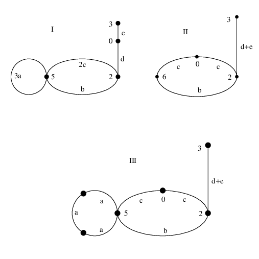
In this example, we consider a pm-graph (Γ,q)(\Gamma,\textbf{q}) as the graph II in Figure 2, where the edge lengths and the values of q are illustrated. In this case, Γ\Gamma has a self loop and two multiple edges. We first ignore the vertex with q value 00 and valence 22. To avoid having multiple edges, we add a vertex to one of the multiple edges such that the added vertex has q value 00. We can deal with the self loop by either applying Equation (10) or considering two additional vertex with q value 00 on the self loop. These cases are illustrated by graphs I​III and I​I​IIII in Figure 2. Thus, we can compute polarized metrized graph invariants of Γ\Gamma in two different ways, and the results are as follows:

τ⁡(Γ)\displaystyle\tau(\Gamma) =b+2​c+3​(a+A)12,\displaystyle=\frac{b+2c+3(a+A)}{12}, θ⁡(Γ)\displaystyle\theta(\Gamma) =480​b​cb+2​c+170​A,\displaystyle=\frac{480bc}{b+2c}+170A,
φ⁡(Γ)\displaystyle\varphi(\Gamma) =11​a24+11​b2+764​b​c+44​c272​(b+2​c)+9​A2,\displaystyle=\frac{11a}{24}+\frac{11b^{2}+764bc+44c^{2}}{72(b+2c)}+\frac{9A}{2}, λ⁡(Γ)\displaystyle\lambda(\Gamma) =9​a25+3​(b2+24​b​c+4​c2)25​(b+2​c)+27​A25,\displaystyle=\frac{9a}{25}+\frac{3(b^{2}+24bc+4c^{2})}{25(b+2c)}+\frac{27A}{25},
ϵ⁡(Γ)\displaystyle\epsilon(\Gamma) =11​a12+11​b2+764​b​c+44​c236​(b+2​c)+8​A,\displaystyle=\frac{11a}{12}+\frac{11b^{2}+764bc+44c^{2}}{36(b+2c)}+8A, Z⁡(Γ)\displaystyle Z(\Gamma) =23​a576+23​b2+812​b​c+92​c21728​(b+2​c)+3​A16,\displaystyle=\frac{23a}{576}+\frac{23b^{2}+812bc+92c^{2}}{1728(b+2c)}+\frac{3A}{16},

where A=d+eA=d+e, ℓ⁡(Γ)=3​a+b+2​c+d+e\ell(\Gamma)=3a+b+2c+d+e, g⁡(Γ)=2g(\Gamma)=2 and g¯​(Γ)=12\bar{g}(\Gamma)=12.

Refer to caption
Figure 2. A pm-graph with a self loop, nonzero q and two multiple edges.

The following example is about the computation of invariants of a class of simple pm-graphs. It is given to show both symbolic computations and different aspects of numerical computations which would be critical during the implementation of our algorithm.

Example 4:

A ladder graph Ln​(a,b)L_{n}(a,b) is planar graph that looks like a ladder with nn rungs. It has 2​n2n vertices and 3​n−23n-2 edges. Edges looking like rungs are of lengths bb, and each of the remaining 2​(n−1)2(n-1) edges has length aa. Thus, ℓ⁡(Ln​(a,b))=2​(n−1)​a+n​b\ell(L_{n}(a,b))=2(n-1)a+nb and g⁡(Γ)=n−1g(\Gamma)=n-1. Figure 3 shows an example. Using the same notation for the corresponding simple pm-graph, we obtain the results given in the tables below:

Refer to caption
Figure 3. Ladder graph L3​(a,b)L_{3}(a,b).
nn e v g​(Ln​(a,b))g(L_{n}(a,b)) ℓ​(Ln​(a,b))\ell(L_{n}(a,b))
22 4 4 1 2​(a+b)2(a+b)
33 7 6 2 4​a+3​b4a+3b
44 10 8 3 2​(3​a+2​b)2(3a+2b)
55 13 10 4 8​a+5​b8a+5b
Table 1. Number of edges, vertices, genus and length of Ln​(a,b)L_{n}(a,b) for n∈{2, 3, 4, 5}n\in\{2,\,3,\,4,\,5\}.

We used Mathematica [19] to do the symbolic computations given in Tables 2, 3 and 4. As the number of vertices gets larger the expressions in the results become more complicated, so we listed the results only for small values of nn.

nn τ⁡(Γ)ℓ⁡(Γ)\frac{\tau(\Gamma)}{\ell(\Gamma)} θ⁡(Γ)OPENℓ⁡(Γ))\frac{\theta(\Gamma)}{\ell(\Gamma))}
22 112\frac{1}{12} 00
33 8​a2+14​a​b+7​b212​(2​a+3​b)​(4​a+3​b)\frac{8a^{2}+14ab+7b^{2}}{12(2a+3b)(4a+3b)} 2​b​(2​a+b)(2​a+3​b)​(4​a+3​b)\frac{2b(2a+b)}{(2a+3b)(4a+3b)}
44 12​a4+36​a3​b+38​a2​b2+18​a​b3+3​b424​(a+b)​(3​a+2​b)​(2​a2+4​a​b+b2)\frac{12a^{4}+36a^{3}b+38a^{2}b^{2}+18ab^{3}+3b^{4}}{24(a+b)(3a+2b)(2a^{2}+4ab+b^{2})} 4​a4+20​a3​b+26​a2​b2+10​a​b3+b4(a+b)​(3​a+2​b)​(2​a2+4​a​b+b2)\frac{4a^{4}+20a^{3}b+26a^{2}b^{2}+10ab^{3}+b^{4}}{(a+b)(3a+2b)(2a^{2}+4ab+b^{2})}
55 128​a5+496​a4​b+704​a3​b2+476​a2​b3+160​a​b4+19​b512​(8​a+5​b)​(4​a2+6​a​b+b2)​(4​a2+10​a​b+5​b2)\frac{128a^{5}+496a^{4}b+704a^{3}b^{2}+476a^{2}b^{3}+160ab^{4}+19b^{5}}{12(8a+5b)(4a^{2}+6ab+b^{2})(4a^{2}+10ab+5b^{2})} 2​(128​a5+656​a4​b+1104​a3​b2+716​a2​b3+160​a​b4+9​b5)(8​a+5​b)​(4​a2+6​a​b+b2)​(4​a2+10​a​b+5​b2)\frac{2(128a^{5}+656a^{4}b+1104a^{3}b^{2}+716a^{2}b^{3}+160ab^{4}+9b^{5})}{(8a+5b)(4a^{2}+6ab+b^{2})(4a^{2}+10ab+5b^{2})}
Table 2. For pm-graph Γ=Ln​(a,b)\Gamma=L_{n}(a,b), τ⁡(Γ)\tau(\Gamma) and θ⁡(Γ)\theta(\Gamma) for n∈{2, 3, 4, 5}n\in\{2,\,3,\,4,\,5\}.
nn φ⁡(Γ)ℓ⁡(Γ)\frac{\varphi(\Gamma)}{\ell(\Gamma)} λ⁡(Γ)ℓ⁡(Γ)\frac{\lambda(\Gamma)}{\ell(\Gamma)}
22 00 112\frac{1}{12}
33 2​a2+2​a​b+b23​(2​a+3​b)​(4​a+3​b)\frac{2a^{2}+2ab+b^{2}}{3(2a+3b)(4a+3b)} 110\frac{1}{10}
44 72​a4+192​a3​b+164​a2​b2+60​a​b3+9​b472​(a+b)​(3​a+2​b)​(2​a2+4​a​b+b2)\frac{72a^{4}+192a^{3}b+164a^{2}b^{2}+60ab^{3}+9b^{4}}{72(a+b)(3a+2b)(2a^{2}+4ab+b^{2})} 5​a+3​b14​(3​a+2​b)\frac{5a+3b}{14(3a+2b)}
55 (2​a+b)​(16​a4+52​a3​b+51​a2​b2+16​a​b3+2​b4)(8​a+5​b)​(4​a2+6​a​b+b2)​(4​a2+10​a​b+5​b2)\frac{(2a+b)(16a^{4}+52a^{3}b+51a^{2}b^{2}+16ab^{3}+2b^{4})}{(8a+5b)(4a^{2}+6ab+b^{2})(4a^{2}+10ab+5b^{2})} 5​(2​a+b)9​(8​a+5​b)\frac{5(2a+b)}{9(8a+5b)}
Table 3. For pm-graph Γ=Ln​(a,b)\Gamma=L_{n}(a,b), φ⁡(Γ)\varphi(\Gamma) and λ⁡(Γ)\lambda(\Gamma) for n∈{2, 3, 4, 5}n\in\{2,\,3,\,4,\,5\}.
nn ϵ⁡(Γ)ℓ⁡(Γ)\frac{\epsilon(\Gamma)}{\ell(\Gamma)} Z⁡(Γ)ℓ⁡(Γ)\frac{Z(\Gamma)}{\ell(\Gamma)}
22 00 112\frac{1}{12}
33 4​a2+10​a​b+5​b23​(2​a+3​b)​(4​a+3​b)\frac{4a^{2}+10ab+5b^{2}}{3(2a+3b)(4a+3b)} (a+b)22​(2​a+3​b)​(4​a+3​b)\frac{(a+b)^{2}}{2(2a+3b)(4a+3b)}
44 36​a4+132​a3​b+154​a2​b2+66​a​b3+9​b418​(a+b)​(3​a+2​b)​(2​a2+4​a​b+b2)\frac{36a^{4}+132a^{3}b+154a^{2}b^{2}+66ab^{3}+9b^{4}}{18(a+b)(3a+2b)(2a^{2}+4ab+b^{2})} 36​a4+120​a3​b+134​a2​b2+60​a​b3+9​b4108​(a+b)​(3​a+2​b)​(2​a2+4​a​b+b2)\frac{36a^{4}+120a^{3}b+134a^{2}b^{2}+60ab^{3}+9b^{4}}{108(a+b)(3a+2b)(2a^{2}+4ab+b^{2})}
55 64​a5+288​a4​b+452​a3​b2+298​a2​b3+80​a​b4+7​b5(8​a+5​b)​(4​a2+6​a​b+b2)​(4​a2+10​a​b+5​b2)\frac{64a^{5}+288a^{4}b+452a^{3}b^{2}+298a^{2}b^{3}+80ab^{4}+7b^{5}}{(8a+5b)(4a^{2}+6ab+b^{2})(4a^{2}+10ab+5b^{2})} 5​(2​a+b)​(16​a4+60​a3​b+73​a2​b2+32​a​b3+4​b4)24​(8​a+5​b)​(4​a2+6​a​b+b2)​(4​a2+10​a​b+5​b2)\frac{5(2a+b)(16a^{4}+60a^{3}b+73a^{2}b^{2}+32ab^{3}+4b^{4})}{24(8a+5b)(4a^{2}+6ab+b^{2})(4a^{2}+10ab+5b^{2})}
Table 4. For pm-graph Γ=Ln​(a,b)\Gamma=L_{n}(a,b), ϵ⁡(Γ)\epsilon(\Gamma) and Z⁡(Γ)Z(\Gamma) for n∈{2, 3, 4, 5}n\in\{2,\,3,\,4,\,5\}.

Again we used Mathematica [19] to do exact computations given in Table 5.

nn τ⁡(Γ)ℓ⁡(Γ)\frac{\tau(\Gamma)}{\ell(\Gamma)} θ⁡(Γ)ℓ⁡(Γ)\frac{\theta(\Gamma)}{\ell(\Gamma)} φ⁡(Γ)ℓ⁡(Γ)\frac{\varphi(\Gamma)}{\ell(\Gamma)} λ⁡(Γ)ℓ⁡(Γ)\frac{\lambda(\Gamma)}{\ell(\Gamma)} ϵ⁡(Γ)ℓ⁡(Γ)\frac{\epsilon(\Gamma)}{\ell(\Gamma)} Z⁡(Γ)ℓ⁡(Γ)\frac{Z(\Gamma)}{\ell(\Gamma)}
55 66110868\frac{661}{10868} 55462717\frac{5546}{2717} 4112717\frac{411}{2717} 539\frac{5}{39} 11892717\frac{1189}{2717} 92521736\frac{925}{21736}
1010 210737829\frac{2107}{37829} 55430837829\frac{554308}{37829} 3032971676\frac{30329}{71676} 1576\frac{15}{76} 344578340461\frac{344578}{340461} 2102156128298\frac{210215}{6128298}
1515 306101161956529128700\frac{3061011619}{56529128700} 1809552875784710760725\frac{180955287578}{4710760725} 23843219933411240525\frac{2384321993}{3411240525} 6652494\frac{665}{2494} 15561304120798925975225\frac{155613041207}{98925975225} 295066870992330910210\frac{2950668709}{92330910210}
2020 1052848657811971566979888\frac{105284865781}{1971566979888} 602090570585182148624162\frac{6020905705851}{82148624162} 1218399453275712486590872624\frac{12183994532757}{12486590872624} 3801131\frac{380}{1131} 66526149005373121647718156\frac{6652614900537}{3121647718156} 10979128575725355867839869784\frac{10979128575725}{355867839869784}
Table 5. For pm-graph Γ=Ln​(1,1)\Gamma=L_{n}(1,1), computations of τ⁡(Γ)\tau(\Gamma), θ⁡(Γ)\theta(\Gamma), φ⁡(Γ)\varphi(\Gamma), λ⁡(Γ)\lambda(\Gamma), ϵ⁡(Γ)\epsilon(\Gamma) and Z⁡(Γ)Z(\Gamma) when n∈{5, 10, 15, 20}n\in\{5,\,10,\,15,\,20\}.

Finally, we used Matlab [16], which does machine arithmetic, to obtain the results in Table 6. Note that when n=25000n=25000 in Table 6, Ln​(1,1)L_{n}(1,1) has 5000050000 vertices and 75000−275000-2 edges. As such computations would be possible on a computer with high memory and processing speed, we used Mac Pro with processor 2×2.932\times 2.93 GHz 66-core Intel Xeon (2424 hyper-threading in total) and memory 3232 GB 13331333 MHz DDR3 to obtain these results.

nn τ⁡(Γ)ℓ⁡(Γ)\frac{\tau(\Gamma)}{\ell(\Gamma)} θ⁡(Γ)ℓ⁡(Γ)\frac{\theta(\Gamma)}{\ell(\Gamma)} φ⁡(Γ)ℓ⁡(Γ)\frac{\varphi(\Gamma)}{\ell(\Gamma)} λ⁡(Γ)ℓ⁡(Γ)\frac{\lambda(\Gamma)}{\ell(\Gamma)} ϵ⁡(Γ)ℓ⁡(Γ)\frac{\epsilon(\Gamma)}{\ell(\Gamma)} Z⁡(Γ)ℓ⁡(Γ)\frac{Z(\Gamma)}{\ell(\Gamma)}
500500 0.051341300.05134130 55155.80116855155.801168 27.639727.6397 7.002337.00233 55.471355.4713 0.02789410.0278941
10001000 0.051299780.05129978 221422.325273221422.325273 55.417455.4174 13.946813.9468 111.027111.027 0.02783590.0278359
50005000 0.051266590.05126659 5551550.7777375551550.777737 277.639277.639 69.502369.5023 555.471555.471 0.02778940.0277894
1000010000 0.051262450.05126245 22214198.12118122214198.121181 555.417555.417 138.947138.947 1111.031111.03 0.02778360.0277836
1500015000 0.051261070.05126107 49987945.99147849987945.991478 833.194833.194 208.391208.391 1666.581666.58 0.02778160.0277816
2000020000 0.051260380.05126038 88872829.56381188872829.563811 1110.971110.97 277.835277.835 2222.142222.14 0.02778070.0277807
2500025000 0.051259920.05125992 138868444.360781138868444.360781 1388.751388.75 347.279347.279 2777.692777.69 0.027780.02778
Table 6. For pm-graph Γ=Ln​(1,1)\Gamma=L_{n}(1,1), computations of τ⁡(Γ)\tau(\Gamma), θ⁡(Γ)\theta(\Gamma), φ⁡(Γ)\varphi(\Gamma), λ⁡(Γ)\lambda(\Gamma), ϵ⁡(Γ)\epsilon(\Gamma) and Z⁡(Γ)Z(\Gamma) when n∈{500, 1000, 10000, 15000, 20000, 25000}n\in\{500,\,1000,\,10000,\,15000,\,20000,\,25000\}.

Symbolic computations are clearly the most costly computations. Among the numerical computations, we can have exact arithmetic (arithmetic with numbers having an infinite number of significant figures, i.e, with numbers having infinite precision), precision arithmetic (which involves the numbers with precision more than 1818) and arithmetic with machine numbers.

Acknowledgements: This work is supported by The Scientific and Technological Research Council of Turkey-TUBITAK (Project No: 110T686).

References

  • [1] M. Baker and X. Faber, Metrized graphs, Laplacian operators, and electrical networks, Contemporary Mathematics 415, Proceedings of the Joint Summer Research Conference on Quantum Graphs and Their Applications; Berkolaiko, G; Carlson, R; Fulling, S. A.; Kuchment, P. Snowbird, Utah, 2006, pp. 15-33.
  • [2] M. Baker and R. Rumely, Harmonic analysis on metrized graphs, Canadian J. Math: 59, (2007) No. 2, 225–275.
  • [3] R.B. Bapat, Resistance matrix of a weighted graph, MATCH Commun. Math. Comput. Chem. 50 (2004), 73–82.
  • [4] R.B. Bapat, Resistance distance in graphs, The Mathematics Student, 68 (1999), 87–98.
  • [5] Z. Cinkir, The Tau Constant of Metrized Graphs, Thesis at University of Georgia, Athens, GA., 2007.
  • [6] Z. Cinkir, The tau constant of a metrized graph and its behavior under graph operations, The Electronic Journal of Combinatorics, Volume 18 (1) (2011) P81.
  • [7] Z. Cinkir, The tau constant and the edge connectivity of a metrized graph, submitted. Available at
    http://arxiv.org/abs/0901.1481v2
  • [8] Z. Cinkir, Zhang’s conjecture and the effective Bogomolov conjecture over function fields, Invent. Math., Volume 183, Number 3, (2011) 517–562.
  • [9] Z. Cinkir, The tau constant and the discrete Laplacian matrix of a metrized graph, European Journal of Combinatorics, Volume 32, Issue 4, (2011), 639–655.
  • [10] T. Chinburg and R. Rumely, The capacity pairing, J. reine angew. Math. 434 (1993), 1–44.
  • [11] X. W. C. Faber, The geometric bogomolov conjecture for curves of small genus, Experiment. Math., 18(3):347–367, (2009).
  • [12] X. W. C. Faber, Topics in Arithmetic Geometry over Function Fields, Thesis at Columbia University, New York, NY, 2008.
  • [13] R. D. Jong, Admissible constants of genus 22 curves, Bull. London Math. Soc., 42 (2010) 405-411.
  • [14] R. D. Jong, Second variation of Zhang’s lambda-invariant on the moduli space of curves. To appear in American Journal of Mathematics.
  • [15] D. J. Klein and M. Randić, Resistance distance, Journal Mathematical Chemistry, 12 (1993) 81-95.
  • [16] The MathWorks Inc., Matlab, Version R2011a, Natick, Massachusetts (2011).
  • [17] A. Moriwaki, Bogomolov conjecture over function fields for stable curves with only irreducible fibers, Comp. Math. 105, 125–140. CMP 97:10, (1997).
  • [18] A. Moriwaki, Bogomolov conjecture for curves of genus 22 over function fields, J. Math. Kyoto Univ., 36, 687–695. CMP 97:11, (1996).
  • [19] Wolfram Research, Inc., Mathematica, Version 8.0, Champaign, IL (2010).
  • [20] C. Rao and S. Mitra, Generalized Inverse of Matrices and Its Applications, John Wiley and Sons, 1971.
  • [21] K. Yamaki, Graph invariants and the positivity of the height of the Gross-Schoen cycle for some curves, Manuscripta Mathematica, 131 (2010), 149–177.
  • [22] K. Yamaki, Effective calculation of the geometric height and the Bogomolov conjecture for hyperelliptic curves over function fields, J. Math. Kyoto Univ., 48-2:401–443, (2008).
  • [23] K. Yamaki, Geometric Bogomolov’s conjecture for curves of genus 33 over function fields, J. Math. Kyoto Univ., 42-1:57–81, (2002).
  • [24] S. Zhang, Admissible pairing on a curve, Invent. Math. 112 (1993), 171–193.
  • [25] S. Zhang, Gross–Schoen cycles and dualising sheaves, Invent. Math. 179 (2010), 1–73.