Modulated Reheating and Large Non-Gaussianity
in String Cosmology
Abstract:
A generic feature of the known string inflationary models is that the same physics that makes the inflaton lighter than the Hubble scale during inflation often also makes other scalars this light. These scalars can acquire isocurvature fluctuations during inflation, and given that their VEVs determine the mass spectrum and the coupling constants of the effective low-energy field theory, these fluctuations give rise to couplings and masses that are modulated from one Hubble patch to another. These seem just what is required to obtain primordial adiabatic fluctuations through conversion into density perturbations through the ‘modulation mechanism,’ wherein reheating takes place with different efficiency in different regions of our Universe. Fluctuations generated in this way can generically produce non-gaussianity larger than obtained in single-field slow-roll inflation; potentially observable in the near future. We provide here the first explicit example of the modulation mechanism at work in string cosmology, within the framework of LARGE Volume Type-IIB string flux compactifications. The inflationary dynamics involves two light Kähler moduli: a fibre divisor plays the rôle of the inflaton whose decay rate to visible sector degrees of freedom is modulated by the primordial fluctuations of a blow-up mode (which is made light by the use of poly-instanton corrections). We find the challenges of embedding the mechanism into a concrete UV completion constrains the properties of the non-gaussianity that is found, since for generic values of the underlying parameters, the model predicts a local bi-spectrum with of order ‘a few’. However, a moderate tuning of the parameters gives also rise to explicit examples with potentially observable by the Planck satellite.
1 Introduction
Although initially motivated as a solution to the initial-condition problems of standard Big-Bang cosmology, inflationary models [1] turn out also to provide a successful phenomenological description of the properties of primordial density fluctuations (which are predicted to arise as late-time consequences of quantum fluctuations of the inflaton).
Until relatively recently most of these predictions were made using single-field, slow-roll inflationary models, for which the inflaton is the only light scalar relevant during inflation [2, 3]. The popularity of these models can be traced to several of their attractive features: () simplicity; () effectiveness (they describe primordial fluctuations very well); () predictivity (near, but not exact, scale invariance, scale-independent spectral tilt, gaussian fluctuation statistics, and so on); and () robustness (that is, predictions can be made without knowing the details of the cosmological history between the end of inflation and the beginning of the late-time Big-Bang epoch.)
Why defy Occam?
Despite the simplicity and success of the single-field framework, two independent lines of reasoning suggest exploring multi-field models [4, 5] in more detail. These two lines of reasoning have their roots both in observational developments as well as theoretical considerations, as we now describe.
The first reason to explore more complicated models arises from ongoing improvements in sensitivity of modern observations. In particular, besides testing the consistency of concordance cosmology through improved precision on cosmological parameters [6], new instruments like the Planck satellite [7] will soon probe the existence of non-gaussianity down to a level that can be produced by many types of multi-field models [8, 9] (though not by vanilla single-field slow-roll scenarios). It behooves us as a field to be alive to the kinds of physics to which these measurements might be sensitive, particularly if single-field slow-roll models were to be falsified by the discovery of non-gaussianity.
The second reason to explore more complicated models becomes evident once one tries to integrate inflationary cosmology into our broader understanding of physical law. This raises several independent issues. Most famously, inflationary models require the inflaton to be much lighter than the slowly changing Hubble scale during inflation, . This is a difficult thing to arrange once the inflaton is coupled to any other fields present at the energies of interest, even if these other fields do not play a direct rôle in cosmology [5, 10].
Furthermore, there are very likely to be a good number of other fields to which a putative inflaton might couple, although to make this precise requires specifying a concrete theory. The challenge when doing so is that we do not know the laws of physics at the high energies usually required [11], however the proximity of to and the relevance of quantum fluctuations to primordial fluctuations strongly suggests that it should involve whatever makes sense of quantum gravity at high energies. Since string theory is presently our best-developed framework for understanding quantum gravity, it provides a natural framework for exploring these issues in a crisp way.
And it is in string cosmology that we meet the second reason for exploring multi-field inflationary models in more detail. This is because close to a decade of exploration reveals that multi-field dynamics is the norm for string inflation and not the exception [12]. Although it remains difficult in string theory to achieve a sub-Hubble inflaton mass (and so also slow-roll inflation), once this has been done the same mechanism tends also to drag down the masses of several other fields as well, making them also potentially cosmologically active. This observation — that multi-field models arise fairly generically in this way once embedded into microscopic models — has recently motivated a more detailed study of the systematics of inflationary multi-field dynamics in general [13].
Non-gaussianity and post-inflationary dynamics
One of the main differences between single-field and multi-field inflationary models is the wide variety of fluctuation-generation mechanisms available in the multi-field case. Whereas single-field models must generate adiabatic curvature fluctuations, multi-field models can allow a variety of fluctuations in which the various fields need not alter the gravitational curvature. And although these isocurvature fluctuations would pose an observational problem for Cosmic Microwave Background (CMB) observations if they were to persist to the present epoch, they need not be bad during inflation if they can be converted to adiabatic fluctuations sometime between the epoch of horizon exit and more recent times. This could easily happen, such as if thermal equilibrium were established sufficiently early before the present epoch.
Indeed, generating adiabatic fluctuations through such a roundabout route might even be a virtue rather than a complication, since alternative mechanisms predict primordial fluctuations to depend differently on inflationary properties than the standard single-field mechanism. In particular, the interactions inherent amongst the fields in any multi-field mechanism can often generate observable amounts of non-gaussianity in the CMB, making any discovery of non-gaussianity into a new window into the physics responsible for generating fluctuations, and possibly into some aspects of the post-inflationary regime. Most interestingly, non-gaussianity produced in this way after inflation can often be distinguished observably from non-gaussianity generated directly during inflation, such as by non-standard single-field models [3, 14].
The two best-developed mechanisms for converting, after inflation, inflationary isocurvature perturbations into late-epoch adiabatic fluctuations are the curvaton mechanism [15] and modulation mechanism [16, 17, 18, 19]. One might ask whether these ever arise in string-inflationary models, given the preponderance of multi-field scenarios these models have. Interestingly, they largely do not: for most string-inflation models explored to date only adiabatic fluctuations are appreciably generated at horizon exit, allowing their observational implications to be simply understood in terms of effective single-field models [12, 20].
Isocurvature fluctuations from string vacua
That is not to say that other means for generating fluctuations cannot arise in string theory, and ref. [21] provides a construction of an inflationary cosmology that uses the curvaton mechanism, within an explicit string vacuum in the LARGE Volume Scenario (LVS) [22, 23, 24]. What is perhaps remarkable is that no instances of the modulation mechanism have so far arisen, given that this mechanism was designed with string theory in mind. (The modulation mechanism starts with the observation that couplings in string theory are often given as the values of fields, and so can vary from one Hubble patch to another if these fields so vary. If, in particular, the couplings that vary this way are involved in the transfer of energy from the inflaton into the heat of the later hot Big-Bang epoch, then this reheating would be modulated from one Hubble patch to another, in a way that might describe the observed primordial fluctuations. In particular, such a modulation has been argued generically to produce non-gaussianity at the soon-to-be observable level of [19].)
The goal of this paper is to provide an explicit string realisation of this modulation mechanism, much as ref. [21] did for the curvaton mechanism. We are able to do so, but it proves to be unexpectedly difficult to do, for a variety of reasons. The main reason for this is the difficulty in assembling in one model all of the things that are assumed when building a modulated reheating model: the requirement that inflation takes place in the first place; the presence of a modulating field that is light during inflation, modulates the inflaton decay rate and is almost decoupled from the inflaton; and the conditions required for the modulation mechanism to beat the standard one. Finally, we ask that the modulating field decays before the inflaton, ensuring the absence of any curvaton-like contributions to the generation of the density perturbations.
Here we provide the first explicit string model for which all these conditions apply. By doing so within the LVS we also avoid the need for fine-tuning. What must be chosen carefully, however, is the underlying extra-dimensional manifold, including a particular brane set-up and a particular choice of world-volume fluxes. In particular we make use of novel ingredients in string model building, such as poly-instanton [25] contributions to the superpotential, that allow the exploration of new kinds of phenomenology and cosmology within the LVS [26, 27].
LVS string vacua have several features that make them particularly attractive from the point of view of model building in cosmology. One of these is what makes the LVS attractive for other applications as well: its explicit incorporation of moduli stabilisation within a systematic expansion of the low-energy potential in inverse powers of the extra-dimensional volume. That is, if the extra-dimensional volume (in string units) is , then the LVS scenario starts with the observation that for large the low-energy scalar potential has the generic form of a sum of terms of order , and , where is the dimensionless volume, , of a comparatively small four-cycle in the geometry. For some choices of parameters this has a minimum with , which makes very large volumes natural to obtain.
The low-energy potential, , has another property that is of more specific interest for inflationary applications, however. This is that the leading, , contributions to the potential can be independent of many of the other extra-dimensional moduli, . These moduli therefore can only enter at subdominant order in , in practice arising at one string loop [24]:
| (1) |
where and are calculable functions. For large this allows these moduli to be parametrically light compared with others [28], and in particular to be small compared with the Hubble scale, . This both explains why the inflaton is light [29] and why many other fields are also equally light [21].
In the particular construction explored here, inflation is driven naturally by a fibre modulus — similar to [29] — which acquires a potential from loop corrections, as above. A particular blow-up mode also remains light during inflation since it is stabilised as in [26] due to subleading poly-instanton corrections [25]. The absence of single-instanton contributions to the superpotential for this rigid four-cycle is guaranteed by the presence of extra fermionic zero modes which are Wilson line modulini. Because this blow-up mode is lighter than the Hubble parameter during inflation, it acquires significant isocurvature fluctuations.
The key observation is that this field can play the rôle of a modulation field because its VEV controls the size of the inflaton coupling to visible sector degrees of freedom, resulting in a modulated decay rate due to the fluctuations of the blow-up mode. Reheating takes place as in [30, 31, 32] due to the perturbative decay of the inflaton, converting the initial isocurvature perturbations of the light blow-up mode into adiabatic perturbations that swamp the standard contributions coming from inflationary fluctuations of the inflaton field itself. Finally, couplings of the modulating field also ensure that it decays before the inflaton, ensuring the absence of curvaton-like contributions to primordial density perturbations.
Predictions for non-gaussianity
There are several advantages to having such an explicit UV completion of the modulation mechanism. First, as is often the case, string theory provides a transparent geometrical interpretation of the modulation mechanism in terms of the properties of the internal manifold under consideration. Second, the consistency of the construction sets strong constraints on the final prediction for the non-gaussianities, whose properties we analyse in some detail. In particular, we find non-gaussianities of local form with a bi-spectrum parameter, . Although this is potentially observable by the Planck satellite, we find small tri-spectrum parameters, and .11 1 Such values of tri-spectrum parameters might however be observable by future CMB experiments as EPIC [33] or by large scale structure surveys [34].
The paper is organised as follows. §2 briefly reviews the framework of LVS compactifications on K3 or fibred Calabi-Yau three-folds. With later applications to the modulation mechanism in mind, we choose a manifold with five moduli: the fibre divisor, (which plays the rôle of the inflaton); the modulus of the base of the fibration, (which controls the overall volume ); the first blow-up mode, (whose non-perturbative effects fix the volume at exponentially large values); a second blow-up mode, (which supports the visible sector); and a third blow-up mode, (which intersects and plays the rôle of the modulating field).22 2 Our notation follows ref. [29] as closely as possible. We seek a regime with moduli stabilised with the hierarchy which, because of the LV ‘magic,’ can be done using hierarchies among the input fluxes that are at most .
§3 then describes the inflationary scenario, including a cartoon of how reheating takes place, in order to set up a viable modulation mechanism. In §4 we then describe how primordial fluctuations are generated by the post-inflationary dynamics, showing that the -dependence of the masses and couplings can produce acceptable adiabatic fluctuations from the modulation mechanism. Our conclusions are briefly summarised in §5.
2 The LARGE-volume string inflationary model
In this section, we identify a set of moduli fields with potentially interesting cosmological applications. We derive the leading order contributions to the potential and kinetic terms for these fields, to be used in the next sections for developing a model of inflation accompanied by modulated reheating. We will keep concise in this section, since we mainly apply techniques developed in other works to which we refer.
2.1 Field content
The model we develop requires a compactification based on a Calabi-Yau manifold with a K3 or -fibred structure, characterised by at least five Kähler moduli, two of which are light during inflation and so are relevant for cosmology. We list them here:
- i)
A fibre modulus, , playing the rôle of inflaton field as in [29] and wrapped by a stack of D7-branes.33 3 These D7-branes support a hidden sector since this cycle is non-rigid and tends to be stabilised rather large in string units yielding an exponentially small gauge coupling. The low-energy scalar potential acquires a dependence on through string loop contributions sourced by the D7s [24, 35]. The potential is naturally flat enough to drive inflation.
- ii)
A base modulus, , that mainly controls the overall extra-dimensional volume stabilised at exponentially large values. It is wrapped by the same stack of D7-branes needed to generate the string loop potential for .3 This modulus is heavy during inflation, and lies on its minimum throughout this phase.
- iii)
A blow-up mode , an assisting field required to stabilise the volume at its minimum. Its presence is usual in LARGE volume set-ups. The potential depends on through non-perturbative contributions generated by a stack of D7-branes wrapping and supporting a hidden sector that undergoes double gaugino condensation in a race-track way.44 4 This blow-up mode cannot support a visible sector due to the tension between non-perturbative effects and chirality [36]. It is heavy during inflation.
- iv)
Two intersecting blow-up modes, and . supports a GUT or MSSM-like construction with D7-branes and it is stabilised in the geometric regime by -terms, which render this field heavy during inflation. On the other hand is light during inflation, and plays the rôle of modulating field in our cosmological application. In fact, is wrapped by an Euclidean D3-brane (E3) instanton which generates tiny poly-instantons corrections to the superpotential that fix this modulus at subleading order. Single instanton contributions associated with are absent due to the presence of Wilson line modulini which give rise to extra fermionic zero modes.
2.2 Compactification
In order to realise our scenario, we consider an orientifold of a Calabi-Yau three-fold with a K3 or a fibration structure and .55 5 We focus on orientifold involutions such that , so that . Hence we have five smooth divisors , , whose volumes are given by the real part of the Kähler moduli . The Kähler form can be expanded in a basis of dual two-forms as66 6 We expanded the Kähler form taking a minus sign for , in order to have positive two-cycle volumes also for blow-up modes. .
The volume is expressed in terms of the two-cycle moduli as [37, 38]:
| (2) |
where and given that every Calabi-Yau manifold is characterised by the fact that the signature of the matrix is [39], so with 1 positive and 4 negative signs in our case. The triple intersection numbers are given by 77 7 In the absence of singularities, the triple intersection numbers .:
| (3) |
and are related to the parameters in (2) as follows: , , , , , .
This particular structure of the intersection numbers implies that the is a K3 or divisor fibred over a base whose volume is , is a diagonal del Pezzo divisor, whereas and are two rigid four-cycles intersecting over a two-cycle given by:
| (4) |
We shall also assume that is a rigid four-cycle with Wilson lines, i.e. while (for explicit examples of this kind of divisors in this context see [37]).
The four-cycle moduli are defined as:
| (5) |
and so they take the form:
| (6) | |||||
| (7) | |||||
| (8) |
It is convenient to rewrite the volume in terms of the four-cycle moduli as:
| (9) |
where we set , , , and .
2.3 Brane set-up and fluxes
In this section we shall perform an explicit choice of brane set-up and fluxes that can give rise to the desired phenomenological features of a modulated reheating scenario. We consider the visible sector to be realised by two stacks of D7-branes wrapped around the divisors and 88 8 The suffix ‘vis’ stays for ‘visible’ whereas ‘int’ stays for ‘intersecting’ since we have in mind a GUT-like theory living on with chiral matter arising from an intersection with the stack on . However this set-up contains also the main features of MSSM-like constructions with the visible sector located on both divisors. together with an E3 instanton wrapped around 99 9 We neglect the hidden sector D7-branes wrapped around and (in order to yield the loop generated inflationary potential) and (in order to yield the racetrack superpotential) since they do not play any rôle in the modulation mechanism.:
| (10) |
We also turn on the following world-volume fluxes:
| (11) |
where the half-integer contributions come from the cancellation of the Freed-Witten anomalies. Let us fix the -field in order to cancel the total flux on so that the instanton contributes to the superpotential. Hence we choose which gives rise to the following total world-volume fluxes: 1010 10 Even though we are focusing on orientifold involutions such that , the -field is not completely projected out, since it can have non-zero discrete coefficients which can compensate the half-integer contribution in .
The presence of non-vanishing gauge fluxes has four implications:
- 1.
They induce -charges for the Kähler moduli. The charges of the blow-up moduli and under the diagonal of the D7-stacks wrapping and read:
(12) These charges can be written one in terms of the other as:
(13) - 2.
The gauge coupling of the field theory on the D7-stack wrapping the divisor acquires a flux-dependent shift. In fact, the gauge coupling is given by:
(14) where is the real part of the axio-dilaton, while the flux-dependent factor is:
- 3.
The world-volume fluxes generate moduli-dependent Fayet-Iliopoulos (FI) terms which take the form:
(15) (16) where we denoted with the Kähler potential of the 4D effective theory.
- 4.
The chiral intersections between different stacks of D7-branes depend on the gauge fluxes in the following way:
In order to have an instanton contributing to the superpotential we need to kill its chiral intersections with the visible sector (and preferably also with any other sector of the theory). These chiral intersections, if non-vanishing, tend to destroy the instanton contribution, since they would lead to a superpotential of the form , where the correspond to open string matter fields, charged under the visible sector gauge group. In order to preserve the visible sector group, these fields must have zero VEVs resulting in a vanishing [36]. Hence we need to set which implies . On the other hand, we need to have non-vanishing chiral intersections between the D7-stacks on and . This is guaranteed by the relations (13) among the moduli charges which ensure that we can have and while .
Moreover the condition is crucial in order to keep the modulating field light. In fact, the FI terms (15) and (16), generically introduce a dependence on both and the combination
| (17) |
since
| (18) |
Therefore both of these fields would get a very large mass. However, the condition implies that and introduce a dependence in the -term potential only on the combination , leaving as a flat direction. This discussion allows to appreciate the essential rôle of the intersection between the two cycles and : thanks to this structure we are left with a flat direction that we can then use for cosmological purposes.
In order to simplify the system under consideration, we shall also require which implies and . The final condition written in terms of flux quanta and wrapping numbers reads:
| (19) |
which leads to:
Illustrative flux choice
An illustrative choice of fluxes that leads to and gives rise to three families of chiral matter (i.e. ) is:
| (20) |
The corresponding divisors (which we assume to be smooth) wrapped by the visible sector and the intersecting D7-stack are:
| (21) |
and
| (22) |
which, from the condition (19), implies . The resulting charge , flux-dependent shift and FI-term for the visible sector become:
| (23) |
2.4 Supergravity effective action
Let us now outline the main features of the effective low-energy 4D supergravity model derived by compactifying over the manifold described in section 2.2. After including the leading perturbative corrections, the Kähler potential is (we work throughout in the 4D Einstein frame):
| (24) |
The corrections are controlled by the quantity , where is the Euler number of the compact manifold while the one-loop open string corrections take the form studied in [35].
The non-perturbative superpotential is assumed to have a racetrack dependence on , with additional poly-instantons corrections on :1111 11 The non-perturbative corrections dependent on the large cycles and are negligible and are likely to be absent since these are non-rigid cycles.
| (25) |
The superpotential is characterised by the constant , associated with the tree-level flux stabilisation of the dilaton and the complex structure moduli, and by the non-perturbative corrections weighted by the constants and . The parameters and are given by and and arise due to gaugino condensation on D7-branes (with and being the rank of the associated gauge group). The rôle of the racetrack form for the superpotential will become clear in section 2.6.
Even though is a rigid cycle (), single instanton contributions to the superpotential are absent, due to the presence of extra fermionic zero modes which are Wilson line modulini (). However, this zero mode structure can give rise to instanton corrections to the gauge kinetic functions of the field theories living on : this is the origin of the so-called ‘poly-instanton’ corrections which depend on . These tiny non-perturbative effects could be killed by the presence of chiral intersections between the E3 instanton on and visible sector fields living on the cycle that intersects . We have however chosen the gauge fluxes appropriately so to cancel these chiral intersections. Moreover, this set-up would normally generate -dependent loop corrections, which can in principle render this blow-up mode heavy. However, for appropriate choices of fluxes, the loops depend on the same combination of four-cycles fixed by the -terms, and so a flat direction remains in the (, ) plane. We discuss this issue in the next subsection.
2.5 D-term stabilisation
We recall that is the rigid four-cycle supporting a GUT or MSSM-like model in terms of wrapped D7-branes. It has been shown in [36] that the cycle supporting chiral matter cannot get any non-perturbative correction, since an instanton wrapped around would generically have chiral intersections with visible sector fields. Therefore the corresponding modulus has to be fixed using different effects [38]. This is what we are going to analyse here, exploiting the field dependence of the -term potential, and of subleading (but crucial) string loop contributions.
The world-volume flux generates a modulus-dependent FI-term . The resulting -term potential provides the leading order effect that depends on and :
| (26) |
where the gauge coupling is given by . In the expression (26) we include also the possible presence of canonically normalised visible sector singlets (open string states) with corresponding charges given by .
We focus on supersymmetric minima where , for the following reason. The total scalar potential includes also -term contributions from the matter fields:
| (27) |
where the are positive numbers, and denotes the scalar potential for the remaining Kähler moduli that we will analyse in detail in the next sections. Given that in a LARGE volume expansion whereas (as we shall see in the next section), a non-vanishing would give rise to a dangerous run-away behavior for the volume mode, that must be avoided.
Hence we shall look for non-supersymmetric minima where is vanishing up to corrections. The leading order cancellation of the FI-term can be achieved in two ways. First, the case in which and ; second, the case where and , where is a visible sector singlet (like a right-handed sneutrino for example) and . The first case would fix the combination without forcing any divisor to shrink to zero size. However, the two-cycle would reach the wall of the Kähler cone, i.e. , resulting in a lack of control over the effective field theory. We need therefore to focus on the second case where a singlet acquires a non-zero VEV. The minimum for is located at (for ):
| (28) |
Substituting this value in the total scalar potential we find:
| (29) |
As we shall see in the next section, the Hubble constant during inflation scales as (setting ), whereas the mass-squared of the canonically normalised modulating field scales as . This implies that in order to have a light modulating field, the potential for this field has to be developed at order . However the potential (29) introduces a dependence on the combination at order which would render the modulating field too heavy if . Hence we have to perform a very moderate tuning of of the order . 1212 12 In the next section, we shall fix this leading order flat direction via a poly-instanton generated potential which scales as and so we shall, more correctly, tune such that . Moreover, the modulating field could be kept light also by choosing and such that the combination (i.e. and ). However we do not consider this option since it would lead to a modulation mechanism which would not be able to beat the standard mechanism for the production of the density perturbations.
After having analysed -term and matter field -term contributions to the potential for , we examine how it is influenced by string loop corrections, showing that the latter are able to fix this combination. Given that each cycle wrapped by a stack of D7-branes receives one-loop open string corrections [24, 35], one would expect effects of order which depend on both and . However, the coefficients of these corrections can be appropriately tuned so that at leading order they depend only on the combination , whereas all the other terms are very suppressed. The leading order loop correction then reads [35]:
| (30) |
These loop effects can indeed compete with the -dependent -term piece in (29). The complete scalar potential for the combination is then constituted by the sum of all contributions:
| (31) |
and it admits a minimum at . If we integrate out and place it to its minimum we are left with a volume dependent potential of the form:
| (32) |
that is proportional to . This shows that, as anticipated, -term, -term, and string loop contributions to the moduli potential stabilise the linear combination , leaving a leading order flat direction which will be softly lifted by polyinstanton corrections, and will play the rôle or our modulating field.
2.6 F-term stabilisation
We now study the structure of the -term scalar potential for the Kähler moduli using the Kähler potential and the superpotential of eqs. (24) and (25). We follow the discussion of ref. [29] and [26]. The scalar potential can be organised in an expansion in inverse powers of the volume:
| (33) |
where is a number that depends on the parameters of the model (more on this later). We now discuss the previous potential order by order in the expansion, showing that at each order it can provide stable minima for some of the moduli.
Moduli stabilisation at
After minimising the axionic direction, as usual in models based on LVS, and trading for the volume (in the limit in which for ), the leading order contribution to the -term scalar potential can be readily calculated and results: 1313 13 Since does not play any relevant rôle in the discussion, from now on we use it to set to simplify some of the formulae. Moreover, we neglect the overall normalisation factor [21].
| (34) | |||||
The scalar potential, at this order in the expansion, contains terms with different signs associated with the racetrack structure of the superpotential. Eq. (34) does not depend on the fibre modulus [29], nor on the blow-up mode supporting the poly-instanton corrections [26]. It does not do so because the dominant contribution to the potential of arises via string loops [24] at order . As we show later, develops a potential at even more subleading order, , where is a parameter that assumes values larger than .
On the other hand, as we learned in the previous section, combined effects of -term, -term, and string loop contributions do stabilise the combination : upon integrating it out, we are left with a volume dependent contribution to the potential summarised in eq. (32), which can be simply regarded as a shift of the correction term:
| (35) |
We now focus on the potential (34), replacing with . In order to express the conditions for the stabilisation of and in a compact way, it is convenient to introduce the quantity . The vanishing of the first derivatives of with respect to and provides the following extrema for and (keeping the first order contributions in an expansion in and ):
| (36) |
where
| (37) |
and
| (38) |
with for large . We also impose that is positive in order to have a minimum in the -axion direction. The extrema associated with equation (36) correspond to stable minima both for the volume (or alternatively the field ) and the field . These formulae show that the volume is LARGE thanks to an exponential dependence on the parameters of the model.
Notice that in the case of single exponential (), (38) reduces to , implying that for (the limit of large volume we are interested in) the corrections to due to are always subleading. As we will discuss in what follows, the consistency of our approximations requires to avoid this, and so we set . We finally point out that this minimum is AdS and so additional uplifting terms are needed to uplift the potential to a nearly Minkowski vacuum (for explicit de Sitter examples see [40]).
Moduli stabilisation at order
Each cycle wrapped by a stack of D7-branes receives one-loop open string corrections [24, 35] which, as pointed out in [29], generate a subleading potential for . This potential, for a certain range of , results flat enough to be suitable for inflation. In this subsection we focus only on the and -dependent loop corrections which can be estimated using a procedure identical to [29]:
| (39) |
where , , are given by:
| (40) |
where , , and are constants that depend on the VEV of the complex structure moduli which have been fixed at tree level (see [29] for more details). In what follows we regard these constants as free, to be fixed using consistency or phenomenological requirements. When , the minimum for is at:
| (41) |
justifying the scaling of (39). In the following, for definiteness, we consider the case .
Moduli stabilisation at
The leading order contribution to the scalar potential from the -dependent poly-instanton corrections turns out to be more suppressed than the ones analysed in the previous subsection since it scales as [26]:
| (42) | |||||
where we have neglected -independent pieces in , since they are not relevant for moduli stabilisation. Substituting (36) in (42), we obtain a very compact expression
| (43) |
where
| (44) |
The potential (43) for admits a minimum at and so it scales as (the value of determines the depth of the vacuum).
At this point, we can finally fully appreciate the rôle of the racetrack form of the superpotential. Let us consider the contributions proportional to to the parameter
| (45) |
In the single exponential case (setting ), becomes negative with an absolute value smaller than unity:
| (46) |
and so we end up in a regime where the minimum for is out of the Kähler cone. However in the racetrack case it is possible to render positive and large enough to trust the effective field theory. As we will learn in section 3.3, a value of in the interval is preferred for our cosmological applications. Many possibilities exist, although the choice of the parameters have to be carefully balanced in order to get the desired result. Focusing on the illustrative flux choice of section 2.3, we present here a parameter fit that provides an acceptable minimum for , and a value of in the preferred range (recall that and ):
| (47) |
This choice of parameters yields the following value for the VEVs of the fields at the minimum:
| (48) | |||||
Notice that lies in the interval preferred by our cosmological applications. Since it is larger than , the resulting potential for the field is suppressed by higher powers of the volume with respect to the string-loop potential. Moreover our choice of guarantees that the term in (29) proportional to which arises from the non-exact cancellation of the -term potential, does not beat the poly-instanton potential. In fact, this requirement turns into the condition .
This fit determines and fixes most of the available parameters in this set-up, and has also interesting cosmological consequences as we will discuss in section 4.2. The only exceptions are parameters characterising the geometry and , and the parameter characterising the string loop potential. In what follows, we will fix the quantities as in the previous fit and use the remaining undetermined parameters to further characterise the predictions for the cosmological model of interest.
2.7 Kinetic terms and canonical normalisation
After determining an expression for the potential, we need to analyse the kinetic terms in order to canonically normalise the fields. As for the potential, also the kinetic Lagrangian can be organised in terms of an expansion in inverse powers of the volume:
| (49) |
We analyse in detail the procedure to render canonical the kinetic terms in appendix A. There we show how to define new canonically normalised fields, dubbed , , , , . In terms of these fields, the kinetic Lagrangian, up to second order in inverse powers of the volume, reads simply:
| (50) |
Here we only present the results, and write the relations between the original fields and the canonically normalised fields (trading for ):
| (51) | |||||
| (52) | |||||
| (53) | |||||
| (54) | |||||
| (55) |
where the function is a subleading correction which in the limit of exponentially large volume and large takes the form:
| (56) |
Notice that the combination can be written in terms of the canonically normalised fields as
| (57) |
whereas the leading order volume scaling of the minimum of the canonically normalised fields is:
| (58) |
where the values of the original fields at their minimum, as obtained in the previous subsections, are given by (at leading order in the volume):
| (59) |
3 Inflationary and post-inflationary dynamics
After having acquainted a good theoretical control on the scalar potential and kinetic terms, we turn to study how inflation is realised in this set-up.
3.1 Moduli dynamics during inflation
We assume that inflation occurs while one of the moduli we consider is rolling over the potential to reach its minimum. In our set-up, we have two light moduli that can have interesting cosmological applications: and . For our purposes, as we discuss in section 4.1, the best candidate for driving the inflationary process is the field , while the field modulates the reheating process.1414 14 The possibility to drive inflation using the field controlled by poly-instanton corrections has been recently studied in [27]. We can assume that the fields , and lie at their minima during inflation: we check later that these fields have indeed masses much larger than the Hubble scale during inflation, so this hypothesis is correct.
We start discussing the inflationary dynamics. Since the potential for the inflationary field is controlled by string loop contributions, the inflationary dynamics is very similar to the one of fibre inflation [29]. Expanding in terms of its canonically normalised counterpart (and writing to denote the classical shift of some field from its minimum) allows to write, at leading order in inverse powers of the volume:
| (60) |
The potential for the field is provided by string loops corrections, as we discussed in section 2.6. It is given by eq. (39), expressing in terms of the canonically normalised field :1515 15 We introduced the overall normalisation factor (see [21]). Unless otherwise stated, we set the Planck mass .
| (61) |
with (see eq. (41)) for . Most of the parameters appearing in the previous potential are fixed by the fit in eq. (47), that is by the requirement of having controlled minima for the stabilised moduli.
The slow roll parameters derived from the inflationary potential (61) take the form [29]:
| (62) | |||
| (63) |
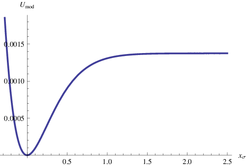
Inflation occurs when and , which happens in a region where the potential is sufficiently flat (see Fig.1). From the expressions above, one notices that a sufficient condition to ensure this is and . The number of e-foldings is given by:
where starred quantities are evaluated at horizon exit. During the inflationary period, the Hubble parameter is given by the following expression:
| (64) |
Notice that it scales with the volume as , a reference scale for the remaining discussion.
Armed with these preliminary definitions, and using the parameter fit of eq. (47), we can determine an inflationary trajectory characterised by the following features:
| (65) |
which yield:
| (66) |
Notice that once has been fixed, all the quantities characterising the inflationary process are determined. We get a reduced amplitude of the scalar power spectrum, defined as:
| (67) |
with respect to the COBE normalisation . This is not a problem since the curvature perturbations will be produced by the alternative mechanism of modulated reheating, as we are going to discuss in section 4. Notice that the value of the parameter is relatively large in this set-up, as in fibre inflation [29]. In the case in which the inflaton provides the dominant contribution to the curvature fluctuations, this would imply that the tensor-to-scalar ratio is large (this was indeed one of the motivations to study fibre inflation [29]); in our context, this is not so since the curvature perturbations are produced by a different mechanism. Nevertheless, having a large will be important for having a successful scenario of modulated reheating.
During inflation, the masses of the -fields, once canonically normalised, scale with the volume as:1616 16 The volume scalings of the various fields can be understood as follows: from (113), at leading order is mostly the overall volume which is stabilised at order . Both (mostly given by as can be seen from (119)) and (mostly given by as can be seen still from (119)) are fixed at order . The potential for is discussed next.
| (68) |
For our large value of the volume, , and have masses larger than the Hubble parameter during inflation: this shows that our hypothesis that they sit on their minima is consistent. The field can instead be light during inflation, for our value of . The potential for is calculated starting from the potential for the field , analysed in section 2.6. Expanding the modulating field as , the field is given in terms of its canonically normalised counterpart by:
| (69) |
The requirement of having a trustable effective field theory sets two new constraints on the value of the displacement from the minimum which take the form:
| (70) | |||||
| (71) |
Therefore, from eq. (43), we obtain the following potential for the modulating field, valid in regions of where the previous constraints hold:1717 17 We are neglecting possible up-lifting contributions to the modulating field potential since they are irrelevant for the present discussion.
| (72) |
We point out that the potentials for the inflaton and the modulating field are decoupled in this set-up, and so the two fields can evolve independently in field space. This is also clear from the fact that does not depend on , as we showed in section 2.6. The potentials are plotted in Fig 1 for a representative choice of parameters.
In the following, we focus on the positive range for , where is bounded from above. The quantities and depend on the microscopic properties of the model, and for the parameter fit of eq. (47) they take the values and .
We finally point out that the mass of the modulating field for an arbitrarily large value of is given by:
| (73) |
As we have seen, . Thus if this mass is smaller than the Hubble parameter during inflation, and the field is light during this phase. Our choice of parameters ensures that this condition holds since we shall find that the requirement of generating enough density perturbations fixes . Hence we get that is satisfied for our value .
The fact that is an essential property to implement modulated reheating since it ensures that the field is practically frozen at the classical level but it develops a scale invariant spectrum of quantum fluctuations with amplitude set by the Hubble scale: . The other crucial feature to realise the modulation mechanism is to have a -dependent inflaton coupling to visible degrees of freedom so that the oscillations of can indeed modulate the decay rate of the inflaton that gives rise to reheating. We investigate this key property of our model in the next sections.

3.2 Inflationary couplings to observable sectors
An essential feature of the LVS framework is that we can compute the volume scaling of the couplings between the moduli (among which the inflaton) and all the other visible or hidden degrees of freedom localised on D7-branes wrapped on internal four-cycles [23, 32, 41]. This is a necessary ingredient for being able to calculate the inflaton decay rates into visible degrees of freedom. This allows us to understand the dynamics of reheating at the end of inflation [32], in particular to determine whether a modulated reheating scenario can be successfully implemented in our set-up.
We focus on the decay channels of the moduli fields into light gauge bosons living on the D7-worldvolumes. As described in [23, 32, 41], the corresponding couplings can be derived from the moduli dependence of the tree-level gauge kinetic function given by eq. (14). The relevant kinetic terms read (writing ):
| (74) |
While the inflaton oscillates around its minimum after inflation ends, we consider the moduli as quantum fields expanded around a classical value:
where we take into account the possibility that classical VEVs are shifted from the minimum during cosmological evolution. Defining the canonically normalised field strength as
| (75) |
we obtain (neglecting the piece involving and taking ):
| (76) | |||||
The moduli couplings to gauge bosons can be obtained by expressing as a function of the canonically normalised fields using the general field redefinitions of eqs. (51)-(55), and expanding each field around its VEV as:
| (77) |
In the previous expression, we included a possible shift from the minimum of the field that is light both during inflation and the reheating process. We instead consider the classical value of the inflaton as coinciding with its minimum in . Indeed, as we know from the study of preheating in LVS [32], the classical homogeneous condensate quickly relaxes to its minimum, and inflaton self-quanta get produced non-perturbatively. Then we can consider as fixed at its minimum during reheating.
As we discussed in section 2, the visible sector fields live on a D7-brane wrapped around the divisor whose volume is given by . Therefore, the couplings of the moduli fields to the visible sector gauge bosons living on can be obtained from [21, 23]:
| (78) |
where the parameters can be obtained from eqs. (54) and (55). Given that their expression is quite long, we relegate it to appendix B. This information is what we need to express the following couplings (denoting as the visible sector gauge bosons and introducing factors of to recast the correct dimensions): 1818 18 The coupling of to visible sector gauge bosons is induced by the mixing between and induced by subleading string loop effects, and it scales as .
| (79) |
The most important one is the coupling of the inflaton field to visible sector gauge bosons since it is this coupling which is responsible for the perturbative decay of the inflaton that reheats the visible sector degrees of freedom. The interesting observation is that this coupling depends on the value of the field , and so it can be modulated by the frozen quantum oscillations of this light field. In fact, it scales schematically as:
| (80) |
where the ’s are positive constants, that can be computed using the formulae of section 2.7. They turn out to be given by:
| (81) |
We stress that only the sign of is fixed and the two constants and depend on the underlying parameters of our model. Choosing:
| (82) |
which give:
| (83) |
we obtain:
| (84) |
The decay rate of the inflaton field into MSSM gauge bosons can be written as:
| (85) |
where the coupling is given by eq. (80), is the mass of the inflaton around its minimum, and is the total number of MSSM gauge bosons.
We conclude pointing out that our brane set-up is such that all the four-cycles are wrapped by stacks of D7-branes. Hence we have also to take into account the moduli couplings to gauge bosons living on all these hidden sectors. Notice that in this case we are interested at the volume scaling of these couplings but not at their exact field dependence since they are not controlling reheating. The volume scaling of the moduli couplings to all gauge bosons present in the model is listed in Table 1. The only issues that remain to be checked are that the inflaton energy is not dumped into hidden, instead of visible, degrees of freedom at the end of inflation [32], and that the modulating field decays before the inflaton. We discuss these points in the next section.
3.3 Reheating
In this section we shall study how reheating takes place, ensuring that the inflaton does not dump all its energy to hidden, instead of visible, degrees of freedom at the end of inflation [32]. Moreover we shall also state the conditions under which the modulating field decays before the inflaton without giving rise to isocurvature contributions.
At the end of inflation, the inflaton field coherently oscillates around its minimum behaving as a classical homogeneous condensate. In the case of blow-up inflation [42], the inflaton energy gets transferred to the visible sector via a first period of preheating [43] characterised by a violent non-perturbative production of inflaton quanta whose perturbative decay subsequently gives rise to reheating [32]. In our case, given that the shape of the inflationary potential for fibre inflation [29] is much less steep than the one for blow-up inflation, we expect a different behaviour for preheating without such a violent non-perturbative production of inflaton inhomogeneities. It might even be that in this case all the dynamics is purely perturbative.
Due to the presence of many hidden sectors in our model, an important issue to check in order to understand reheating, is whether the inflaton decays first to visible or hidden degrees of freedom. As can be seen from Table 1, couples to the hidden gauge bosons living on and more strongly than to the visible gauge bosons living on . Thus the inflaton would naively dump all its energy to hidden, instead of visible, degrees of freedom.
This problem can be solved if the inflaton decay to hidden degrees of freedom is kinematically forbidden. In [32], it has been shown that this is indeed the case if the hidden sector consists of a pure SYM theory that develops a mass gap. From now on, we shall take this as a viable solution. Hence we shall assume that proper non-trivial fluxes can fix the D7-deformation moduli associated with the non-rigidity of and , that would prevent the generation of non-perturbative effects. We also point out that moduli stabilisation is not affected by these new non-perturbative corrections in and since they are subdominant with respect to the string loops in the regime of interest where both of these four-cycles are large. We have to consider a pure SYM theory also on otherwise too much hidden sector dark matter would be produced by the simultaneous inflaton decay to visible and hidden degrees of freedom living on [32].
Under all these constraints on the hidden sector model building, reheating can take place with a temperature of the order:
| (86) |
The requirement of having a reheating temperature above Big Bang Nucleosynthesis, i.e. MeV, sets an upper bound on the value of the overall volume of the order in string units. It is crucial to notice that this bound still allows us to choose values of the volume, , for which the standard mechanism for the generation of the density perturbations can be made negligible. From now on, we shall therefore work in the window , consistent with the parameter choices we made in the previous sections.
Lastly we point out that for an appropriate choice of the parameter , the modulating field decays before the inflaton ensuring that there are no curvaton-like contributions to the generation of the density perturbations from the decay of . In fact, comparing the two decay rates we obtain:
| (87) |
Notice that this upper bound on still allows us to choose values of this parameter, , for which the field is lighter than during inflation and so can act as a modulating field. From now on, we shall therefore work in the window of values for , , or equivalently .
We finally point out that we derived the decay rates (86) and (87) assuming that the modulating field is close to its minimum, i.e. . If this is not the case, a possible worry is that there might be a second period of inflation driven by . However given that decays before this is not the case. In fact, during the initial period of inflation driven by , if , is classically frozen in a region of field space far from its minimum. Then when inflation ends, starts to slowly roll down its potential but is does not drive inflation because all the energy is stored in the inflaton self-quanta which have been produced non-perturbatively at preheating. If such quanta decayed before , then would have enough time to dominate the energy density and drive a second period of inflation but, as we have shown in (87), this does not happen if . Hence for such a value of , while is slow-rolling, the quanta have not decayed yet. Then ends slow-rolling, decays and later on the quanta decay. Thus we need to make sure that decays after not just to neglect curvaton-like contributions but also to ensure the absence of second period of inflation driven by in the case when .
4 Curvature perturbations from modulated reheating
This section describes the generation of primordial fluctuations, first in a general context and then in the specific string-inflation scenario considered above.
4.1 Modulated reheating in LVS inflationary scenarios
Before presenting the details of how curvature perturbations are produced in our set-up, we open this section with a more general discussion on modulated reheating in LVS.
The best moduli candidates to play the rôle of inflaton and modulating fields can be identified by analysing the conditions that these fields have to satisfy to yield a natural realisation of the modulation mechanism:
- 1.
The modulating field must be lighter than the Hubble scale during inflation.
- 2.
The contribution of the modulation mechanism to the spectrum of density perturbations must be larger, or at most equal to the one of the standard mechanism: . These two contributions are given by (at leading order and in the approximation of instantaneous reheating, i.e. ):
(88) where is the decay rate modulated by the fluctuations of the modulating field.
All the decay rates in our model are functions of the mass of the decaying particle and its coupling to gauge bosons, which, in turn, can be functions of the modulating field. As we showed in the previous sections, both the fibre modulus and the blow-up mode can be made lighter than during inflation, so both of these fields satisfy the first condition.
However the field does not satisfy the second one due to the fact that its canonical normalisation makes both its mass (see 61) and its coupling to gauge bosons (see 79 and appendix B) depend exponentially on . This implies that , and so the standard mechanism can never be beaten for the typical inflationary requirement . 1919 19 Inflaton couplings to photons which have an exponential dependence on the modulating field have been discussed in [44] where the authors pointed out that in this case the decay of the inflaton to the modulating field plus two photons dominates over the decay to just two photons. Consequently, the modulating field can behave as dark radiation. It is interesting to notice that our string embedding does indeed include inflaton couplings which depend exponentially on the modulating field as assumed in [44]. However in order to beat the standard mechanism, one needs a dependence of the form where whereas in our case we find .
On the other hand, the different form of the canonical normalisation of a fibre divisor and a blow-up mode, gives rise to a non-exponential dependence of the inflaton coupling to gauge bosons (80) on the blow-up mode , rendering this field a more promising modulating field candidate.
The mass of the inflaton field (see 61) does not depend on , and so we need only to take into account the dependence of the coupling (80) on , obtaining:
| (89) |
From the canonical normalisation (119) we realise that , and so for , (89) reduces to:
| (90) |
regardless of the strength of the modulated coupling! This is due to the fact that comes from the value of the VEV of the canonically normalised blow-up mode even if the modulating coupling (80) is weak since it scales as . This result implies that the ratio between the amplitude of the density perturbations generated by the two mechanisms behaves as:
| (91) |
and so in order to have we need also relatively large.
The value of depends on the nature of the inflaton field. This is the reason why we chose the inflaton as a fibre divisor. In fact, in fibre inflation [29] whereas in blow-up inflation [42] where the inflaton is another blow-up mode. With respect to this, let us present a brief proof of the fact that in blow-up inflation is so small that the modulation mechanism can never beat the standard one. Even assuming a that is the largest possible, i.e. , since goes like [42]:
| (92) |
it turns out that which implies .
We showed why we chose as our inflaton field and as our modulating field. The fact that in fibre inflation [29], implies that in order to get we have to focus on volumes of the order in string units. This is indeed the range that we are considering in our set-up. We point out that the only problem to use a blow-up mode as a modulating field, is to render this field lighter than during inflation given that, in the standard LVS, all the blow-up modes nearby their minima are naturally heavier than the volume mode that sets the scale of the scalar potential. However we showed that this is indeed possible using poly-instanton corrections to the superpotential.
We finally stress that our model represents the first realisation from string theory of a standard modulated reheating scenario where both inflation and the domination over the standard mechanism for the generation of the density perturbations are achieved without requiring any fine-tuning of the underlying parameters.
4.2 Non-gaussianity
The fact that the decay rate of the inflaton field to visible degrees of freedom depends on a light field , has important implications for the generation of adiabatic curvature perturbations . Since is light during inflation, it acquires quantum fluctuations that render its value at horizon exit slightly different in different parts of the Universe. This implies that reheating can occur at different times in different places, depending on the value of . A consequence of this phenomenon is that the isocurvature fluctuations associated with the field can be converted into adiabatic curvature fluctuations . This is the basic idea of the modulated reheating scenario [16, 17, 18] to produce the curvature fluctuations in a way that is alternative to the standard mechanism. This way to produce the curvature fluctuations is particularly interesting, since it can lead to non-gaussianity of local form, with an amplitude much larger with respect to the non-gaussianity normally generated in single field inflation, that are controlled by slow-roll parameters.
In this section, we study in detail the properties of the curvature fluctuations in our set-up. Let us focus on the case in which the modulation of the inflaton decay rate by the field is entirely responsible for producing the adiabatic curvature fluctuation , whose power spectrum matches the COBE normalisation. This is the situation we are considering here, since in our set-up (see eq. (66)) the inflaton contribution to the spectrum of curvature perturbations is negligible.
In our set-up the curvature perturbations are produced by the fluctuations of the decay rate of the inflaton into visible sector fields. Besides the original works on modulated reheating, a careful analysis of how adiabatic perturbations and non-gaussianity are generated is developed for example in [19, 45, 46]. At the linear level, the curvature perturbation is proportional to the spatial variations of the inflaton decay rate:
| (93) |
where the overall factor is calculated by taking into account the dynamics of the inflaton field between the end of inflation and reheating. This value for the overall factor is found in the limit in which the ratio between the inflaton decay rate and the Hubble parameter is very large, a situation that is satisfied in our context.
Going beyond the linear level, one takes a higher order expansion for the curvature perturbations as follows [45]:
| (94) |
The spatial fluctuations in the inflaton decay rate are associated to the spatial fluctuations of the light field during inflation. It is convenient to make an expansion of this quantity in power series of as follows:
| (95) |
We regard as corresponding to the random fluctuation of a light scalar during an inflationary quasi-de Sitter phase, and so we assume that is a Gaussian random variable. The amplitude of the associated two point function is controlled by the Hubble parameter ; odd-point functions and the remaining connected even point functions vanish. Plugging the expression for (95) into eq. (94), we find an expression for as an expansion in that assumes the typical form leading to local non-gaussianity developing after horizon exit [47]. With this form for the curvature perturbation , it is straightforward to calculate the two, three and four point functions of the curvature perturbations to the power spectrum, bispectrum and trispectrum:
| (96) | |||||
| (97) | |||||
| (98) |
We finally express the bispectrum and trispectrum in terms of , and of and . One finds that the power spectrum depends on the first derivative of with respect to :
| (99) |
while the non-gaussianity parameters depend also on higher derivatives of [45]:2020 20 In order to find this result, we have taken the case in which , as shown in [45].
| (100) | |||||
| (101) | |||||
| (102) |
We can then appreciate why non-gaussianity has the opportunity to be much larger than the slow-roll parameters in this context: they depend on quantities (derivatives of ) that do not directly control the inflationary dynamics, nor other aspects of the Universe homogeneous evolution. Consequently, they do not have to satisfy the stringent upper bounds associated with the dynamics of inflation, as happens for example to the non-gaussianity generated by the inflaton field in standard single-field models of inflation, that are controlled by slow-roll parameters.
Plugging the expression for the inflaton decay rate obtained in eq. (85), and using the -dependence of the coupling of eq. (80), we get the following expressions for , and in terms of the underlying parameters:
| (103) | |||||
| (104) | |||||
| (105) | |||||
where , and is the classical shift of the field from its minimum (see discussion after eq. (68)). The shift can be different than zero: since this field is light during inflation, its classical value is frozen during this phase to a position that does not necessarily correspond to its minimum.
We have also to satisfy the constraints in equations (70) and (71). These requirements set stringent constraints on the parameters of the model, and provide very definite predictions on the amount of non-gaussianity produced in this cosmological scenario. On the other hand, the fact that the non-gaussianity parameters and the quantity are non-trivial functions of enriches the phenomenological features of our model. For example, non-gaussianity can exhibit sizeable scale dependence [48], that might be used for further characterising the predictions of our set-up.
In order to generate a power spectrum of curvature fluctuations that matches the COBE normalisation, given our choice of parameters in equation 47, we need to choose:
| (106) |
which gives rise to the following predictions for the parameters controlling local non-gaussianity:
| (107) |
The value of lies very well within the allowed window at confidence level from WMAP7 data [49]. Moreover, our prediction for is large enough to be testable by the Planck satellite which will be able to measure this parameter with an accuracy of the order [50]. On the other hand, and are too small to be detected by the Planck satellite (even if such values for might be observable by future CMB experiments as EPIC [33]). Let us conclude by saying that these values of the non-gaussianity parameters are sensitive to our parameter choice, and so to the geometrical properties of our set-up. By changing the values of the quantities in formula (47) one can obtain different predictions for non-gaussianity: typically, the resulting value of is of order a few. 2121 21 Still detectable by future measurements of the large-scale structure of the Universe that will achieve an accuracy of the order (see [34] for a review). On the other hand, let us emphasise again that the explicit example above shows concretely that non-gaussianity, in our set-up, can be large enough to be observable. This opens up the possibility to have explicit string theory models of cosmology which are testable in the near future.
5 Conclusions
In summary, this paper provides a first realisation of the modulation mechanism within an explicit string inflationary construction, a process which proved surprisingly difficult to achieve given how well-matched the modulation mechanism is (i.e. light fields, VEVs controlling couplings and masses, etc.) to the properties of string theory.
Together with the recent realisation of the curvaton mechanism [21], this provides two instances of string-inflationary models for which primordial fluctuations are generated by converting inflationary isocurvature fluctuations into adiabatic fluctuations during the post-inflationary reheating epoch. But given the apparent ubiquity of light scalar fields during string inflation, these are unlikely to be the last two to be found. More likely, the predominance of standard inflaton-generated fluctuations among string-inflation models is a ‘lamp-post effect,’ reflecting the process through which these models were sought.
The class of inflationary model used here — and in [21] — is driven by the time-evolution of an extra-dimensional modulus, within the context of the LARGE Volume Scenario (LVS) for stabilising string vacua [22]. This is a particularly useful scenario for these purposes, providing as it does a simple and robust mechanism for obtaining exceptionally light scalars [24], whose masses are suppressed relative to other moduli (and to the inflationary Hubble scale [29]) by inverse powers of the large volume. At present, the greatest weakness of these models is our relatively poor understanding of the details of their potential shape, due to the lack of explicit string loop calculations. But the main features, such as the ubiquity of light scalars they predict, depend only on the properties of the tree-level potential and so do not depend on these details.
As ever, although the resulting model is somewhat complicated, several things are gained by embedding a generic inflationary mechanism — like the modulation and curvaton mechanisms for generating primordial fluctuations — into an explicit UV completion, like an explicit string vacuum. Not least among these is the existence proof that the mechanisms can really be viable, given the extreme sensitivity inflation has towards the trickle-down of irrelevant (in the RG sense) gravitational effective interactions to the moderately low energies appropriate to inflation. This includes in particular the ease with which effective ‘Planck slop’ interactions can compete with the inflaton self-couplings, which must be arranged to be small by construction in order to achieve an inflationary slow roll [12].
But other benefits of having a UV completion are also likely to accrue over the somewhat longer term. Among these is the ability to understand the interplay among the conflicting demands put on the microscopic couplings by the sometimes conflicting requirements of successful inflationary phenomenology. In particular, a UV completion is required in order to evaluate the competition among the various fluctuation-generation mechanisms that are at play, to see under which circumstances each can dominate. This is a special case of the broader observation that a proper understanding of reheating requires a complete theory of all of the degrees of freedom that are present at the relevant energies. (A fuller knowledge than just the couplings between the inflaton and observable low-energy fields is required because without knowing all of the degrees of freedom it is impossible to tell whether other channels might too successfully drain away any heat generated by a putative reheating source [32]; what has been called ‘The Parable of the Canadian Winter.’)
Ultimately one hopes having a UV completion to general low-energy mechanisms is a small step on the way towards a longer-term goal: to find a string vacuum that does it all. That is, the challenge of having a multitude of string solutions in the landscape is not that we have too many ways to describe what we find around ourselves; rather, it is that we have not yet found even one way to describe everything we see. The challenge is to find the proverbial needle in the haystack. We believe our best hope to remedy this situation is to identify string ‘modules’: that is, explicit string vacua whose low-energy limits exhibit a host of desirable phenomenological features: the Standard Model, successful inflationary cosmology and reheating, an understanding of dark matter and dark energy, and so on. All of these can put conflicting conditions on the same UV couplings [51], that must simultaneously account for them all. We have seen that though it is possible to obtain large non-gaussianities from string inflation, it is not generic. If non-gaussianities are discovered they would put strong constraints on the proper string compactification eliminating many, but as we have shown, not all of them.
UV completions are also useful for mapping out what can be possible, and this is likely to be a more pressing priority should primordial non-gaussianity be discovered. Such a discovery would immediately precipitate a search for the kinds of mechanisms towards which the evidence points, and by extension also for the kinds of fundamental theories with which they are compatible. Until recently the discovery of observably large, local non-gaussianity could have been inferred as evidence against string theoretical inflationary models, and by extension giving preference for its alternatives [52], given that these alternatives could generate such a non-gaussianity [53] while the only known string inflation-generated sources were not of the local type [14]. This paper, and ref. [21], are first arguments against drawing such a conclusion, and are the first steps towards a broader survey of the string-theoretic options for generating primordial fluctuations.
Acknowledgments
We thank Marta Gómez-Reino for collaboration in the early stages of this work. We would also like to thank Paolo Creminelli, Lev Kofman, Francisco Pedro, Roberto Valandro and David Wands for useful discussions, and Tony Riotto for encouraging us to explore non-standard ways to generate primordial fluctuations. Various combinations of us are grateful for the the support of, and the pleasant environs provided by, the Abdus Salam International Center for Theoretical Physics (ICTP), Perimeter Institute and Cook’s Branch. CB’s research was supported in part by funds from the Natural Sciences and Engineering Research Council (NSERC) of Canada. Research at the Perimeter Institute is supported in part by the Government of Canada through Industry Canada, and by the Province of Ontario through the Ministry of Research and Information (MRI). GT is supported by an UK STFC Advanced Fellowship ST/H005498/1.
Appendix A Kinetic terms for the moduli
In this section we investigate the field redefinitions needed to put the kinetic terms into canonical form. The starting point in the regime of interest is the Kähler metric for the moduli, which is given by the following symmetric matrix:
| (108) |
where, as in [29], we have systematically dropped terms that are suppressed relative to the ones shown by factors .
It is convenient to trade for and for the combination . In the limit in which , are much larger than , and , the kinetic Lagrangian can be canonically normalised order by order in writing:
| (109) |
where the leading term is2222 22 We use units with unless otherwise stated.
| (110) |
while the subleading term at reads
| (111) | |||||
At the transformation
| (112) | |||||
| (113) |
puts the expression (110) into canonical form
| (114) |
where the coefficients , and are obtained from the condition that the matrix satisfies
| (115) |
This has four solutions: , , , , where:
| (116) |
and for concreteness we shall choose the first one will all plus signs. As is shown in [32], the fields and turn out to also diagonalise the mass-squared matrix, in the limit where string-loop corrections to the potential are neglected. Once string-loop corrections are included a subdominant dependence of on also arises and (113) gets modified to:
| (117) |
where is a subleading correction which in the limit of exponentially large volume and large takes the form:
| (118) |
Next we diagonalise the next-order kinetic term, . The first line in (111) becomes diagonal once we rescale the three small moduli as follows
| (119) |
Notice that the original modulus is a combination of and since (119) implies that
| (120) |
The second line in (111) is similarly diagonalised by mixing with . Explicitly, introducing the following subleading corrections to (112):
| (121) |
gives to this order:
| (122) |
Notice that the last two terms in eq. (121) are subleading because for , while from (112) and (113), we have . We can now substitute (117) in (119) to eliminate and directly express , , in terms of the canonically normalised fields:
| (123) |
and
| (124) |
Notice that we have neglected subleading mixing terms between the blow-up modes which will be introduced by subdominant loop corrections. The field redefinitions we have determined render canonical the form of the kinetic terms.
Appendix B Moduli couplings to gauge bosons
In this section, we write the expressions for the parameters introduced in section 3.2, when calculating the moduli couplings to visible sector gauge bosons. They read (here the VEV of the dilaton is simply ):
References
- [1] A. H. Guth, Phys. Rev. D23 (1981) 347; A. D. Linde, Phys. Rev. B108 (1982) 389; A. Albrecht and P. J. Steinhardt, Phys. Rev. Lett. 48 (1982) 1220.
- [2] A. D. Linde, “Particle Physics And Inflationary Cosmology,” Chur, Switzerland: Harwood (1990) 362 p. (Contemporary concepts in physics, 5); D. H. Lyth and A. Riotto, “Particle physics models of inflation and the cosmological density perturbation,” Phys. Rept. 314 (1999) 1 [hep-ph/9807278]; A. Liddle and D. Lyth, “Cosmological Inflation and Large-Scale Structure,” Cambridge University Press (2000); V. Mukhanov, “Physical Foundations of Cosmology,” Cambridge University Press (2005); S. Weinberg, “Cosmology,” Oxford University Press (2008).
- [3] For a particularly model-independent formulation of the predictions of single-field, slow-roll inflationary models, see: C. Cheung, P. Creminelli, A. L. Fitzpatrick, J. Kaplan and L. Senatore, “The Effective Field Theory of Inflation,” JHEP 0803 (2008) 014 [arXiv:0709.0293 [hep-th]].
- [4] A. A. Starobinsky, “Multicomponent de Sitter (Inflationary) Stages and the Generation of Perturbations,” JETP Lett. 42 (1985) 152 [Pisma Zh. Eksp. Teor. Fiz. 42 (1985) 124]; A. D. Linde, “Hybrid inflation,” Phys. Rev. D 49 (1994) 748 [astro-ph/9307002]; J. Garcia-Bellido and D. Wands, “Metric perturbations in two field inflation,” Phys. Rev. D 53 (1996) 5437 [astro-ph/9511029]; A. D. Linde and A. Riotto, “Hybrid inflation in supergravity,” Phys. Rev. D 56 (1997) 1841 [hep-ph/9703209]; M. Sasaki and T. Tanaka, “Superhorizon scale dynamics of multiscalar inflation,” Prog. Theor. Phys. 99 (1998) 763 [gr-qc/9801017]; S. Groot Nibbelink and B. J. W. van Tent, “Scalar perturbations during multiple field slow-roll inflation,” Class. Quant. Grav. 19 (2002) 613 [hep-ph/0107272]; N. Bartolo, S. Matarrese and A. Riotto, “Adiabatic and isocurvature perturbations from inflation: Power spectra and consistency relations,” Phys. Rev. D 64 (2001) 123504 [astro-ph/0107502]; D. Wands, N. Bartolo, S. Matarrese and A. Riotto, “An Observational test of two-field inflation,” Phys. Rev. D 66 (2002) 043520 [astro-ph/0205253]; D. Wands, “Multiple field inflation,” Lect. Notes Phys. 738 (2008) 275 [astro-ph/0702187 [ASTRO-PH]].
- [5] E. J. Copeland, A. R. Liddle, D. H. Lyth, E. D. Stewart and D. Wands, “False vacuum inflation with Einstein gravity,” Phys. Rev. D 49 (1994) 6410 [astro-ph/9401011];
- [6] M. Tegmark et al. [SDSS Collaboration], “Cosmological parameters from SDSS and WMAP,” Phys. Rev. D 69 (2004) 103501 [astro-ph/0310723]; E. Komatsu et al. [WMAP Collaboration], “Five-Year Wilkinson Microwave Anisotropy Probe (WMAP 1 ) Observations:Cosmological Interpretation,” Astrophys. J. Suppl. 180 (2009) 330 [arXiv:0803.0547 [astro-ph]];
- [7] http://www.rssd.esa.int/index.php?project=Planck
- [8] P. Creminelli, A. Nicolis, L. Senatore, M. Tegmark and M. Zaldarriaga, “Limits on non-gaussianities from wmap data,” JCAP 0605 (2006) 004 [astro-ph/0509029]; E. Komatsu, N. Afshordi, N. Bartolo, D. Baumann, J. R. Bond, E. I. Buchbinder, C. T. Byrnes and X. Chen et al., “Non-Gaussianity as a Probe of the Physics of the Primordial Universe and the Astrophysics of the Low Redshift Universe,” arXiv:0902.4759 [astro-ph.CO]; M. Liguori, E. Sefusatti, J. R. Fergusson and E. P. S. Shellard, “Primordial non-Gaussianity and Bispectrum Measurements in the Cosmic Microwave Background and Large-Scale Structure,” arXiv:1001.4707 [astro-ph.CO]; J. Smidt, A. Amblard, A. Cooray, A. Heavens, D. Munshi and P. Serra, “A Measurement of Cubic-Order Primordial Non-Gaussianity ( and ) With WMAP 5-Year Data,” arXiv:1001.5026 [astro-ph.CO]; X. Chen, “Primordial Non-Gaussianities from Inflation Models,” Adv. Astron. 2010 (2010) 638979 [arXiv:1002.1416 [astro-ph.CO]].
- [9] F. Vernizzi and D. Wands, “Non-gaussianities in two-field inflation,” JCAP 0605 (2006) 019 [astro-ph/0603799]; D. Wands, “Local non-Gaussianity from inflation,” Class. Quant. Grav. 27 (2010) 124002 [arXiv:1004.0818 [astro-ph.CO]]; T. Suyama, T. Takahashi, M. Yamaguchi and S. Yokoyama, “On Classification of Models of Large Local-Type Non-Gaussianity,” arXiv:1009.1979 [astro-ph.CO].
- [10] L. Randall, M. Soljacic and A. H. Guth, “Supernatural inflation: Inflation from supersymmetry with no (very) small parameters,” Nucl. Phys. B 472 (1996) 377 [hep-ph/9512439]; P. Binetruy and G. R. Dvali, “D term inflation,” Phys. Lett. B 388 (1996) 241 [hep-ph/9606342]; J. A. Adams, G. G. Ross and S. Sarkar, “Natural supergravity inflation,” Phys. Lett. B 391 (1997) 271 [hep-ph/9608336]; C. P. Burgess, J. M. Cline and R. Holman, “Effective field theories and inflation,” JCAP 0310 (2003) 004 [hep-th/0306079].
- [11] See, however, the following for models that seek inflation at comparatively low energies: D. H. Lyth and E. D. Stewart, “Thermal inflation and the moduli problem,” Phys. Rev. D 53 (1996) 1784 [hep-ph/9510204]; R. Allahverdi, K. Enqvist, J. Garcia-Bellido and A. Mazumdar, “Gauge invariant MSSM inflaton,” Phys. Rev. Lett. 97 (2006) 191304 [hep-ph/0605035]; R. Allahverdi, K. Enqvist, J. Garcia-Bellido, A. Jokinen and A. Mazumdar, JCAP 0706 (2007) 019 [hep-ph/0610134].
- [12]
A. Linde,
“Inflation and string cosmology,”
eConf C040802 (2004) L024
[J. Phys. Conf. Ser. 24 (2005) 151]
[hep-th/0503195];
F. Quevedo, Class. Quant. Grav. 19 (2002) 5721,
[hep-th/0210292];
“The standard model and inflation from string theory,” AIP Conf. Proc. 743 (2005) 341; S. H. Henry Tye, “Brane inflation: String theory viewed from the cosmos,” hep-th/0610221; J. M. Cline, “String cosmology,” hep-th/0612129; R. Kallosh, “On Inflation in String Theory,” hep-th/0702059; L. McAllister and E. Silverstein, “String Cosmology: A Review,” Gen. Rel. Grav. 40 (2008) 565 [arXiv:0710.2951 [hep-th]]; C. P. Burgess, “Lectures on Cosmic Inflation and its Potential Stringy Realizations,” PoS P2GC (2006) 008 [Class. Quant. Grav. 24 (2007 POSCI,CARGESE2007,003.2007) S795] [arXiv:0708.2865 [hep-th]]; D. Baumann, “TASI Lectures on Inflation,” arXiv:0907.5424 [hep-th]. M. Cicoli, “String Loop Moduli Stabilisation and Cosmology in IIB Flux Compactifications,” Fortsch. Phys. 58 (2010) 115 [arXiv:0907.0665 [hep-th]]. C.P. Burgess and L. McAllister, “Challenges for String Cosmology,” Class. Quant. Grav. 28 (2011) 204002 [arXiv:1108.2660]; M. Cicoli and F. Quevedo, “String moduli inflation: An overview,” Class. Quant. Grav. 28 (2011) 204001 [arXiv:1108.2659 [hep-th]]. - [13] H. Y. Chen, J. O. Gong and G. Shiu, “Systematics of multi-field effects at the end of warped brane inflation,” JHEP 0809 (2008) 011 [arXiv:0807.1927 [hep-th]]; X. Chen and Y. Wang, “Large non-Gaussianities with Intermediate Shapes from Quasi-Single Field Inflation,” Phys. Rev. D 81 (2010) 063511 [arXiv:0909.0496 [astro-ph.CO]]; X. Chen and Y. Wang, “Quasi-Single Field Inflation and Non-Gaussianities,” JCAP 1004 (2010) 027 [arXiv:0911.3380 [hep-th]]; A. Achucarro, J. -O. Gong, S. Hardeman, G. A. Palma and S. P. Patil, “Mass hierarchies and non-decoupling in multi-scalar field dynamics,” Phys. Rev. D 84 (2011) 043502 [arXiv:1005.3848 [hep-th]]; “Features of heavy physics in the CMB power spectrum,” JCAP 1101 (2011) 030 [arXiv:1010.3693 [hep-ph]]; N. Agarwal, R. Bean, L. McAllister and G. Xu, “Universality in D-brane Inflation,” JCAP 1109 (2011) 002 [arXiv:1103.2775 [astro-ph.CO]]; G. Shiu and J. Xu, “Effective Field Theory and Decoupling in Multi-field Inflation: An Illustrative Case Study,” arXiv:1108.0981 [hep-th]. C. T. Byrnes and G. Tasinato, “Non-Gaussianity beyond slow roll in multi-field inflation,” JCAP 0908 (2009) 016 [arXiv:0906.0767 [astro-ph.CO]];
- [14] M. Alishahiha, E. Silverstein and D. Tong, “DBI in the sky,” Phys. Rev. D 70 (2004) 123505 [hep-th/0404084]; K. Enqvist and M. S. Sloth, “Adiabatic CMB perturbations in pre big bang string cosmology,” Nucl. Phys. B 626 (2002) 395 [hep-ph/0109214]; R. Flauger, L. McAllister, E. Pajer, A. Westphal and G. Xu, “Oscillations in the CMB from Axion Monodromy Inflation,” arXiv:0907.2916 [hep-th]; R. Flauger and E. Pajer, “Resonant Non-Gaussianity,” arXiv:1002.0833 [hep-th].
- [15] D. H. Lyth and D. Wands, “Generating the curvature perturbation without an inflaton,” Phys. Lett. B 524 (2002) 5 [hep-ph/0110002]; T. Moroi and T. Takahashi, “Effects of cosmological moduli fields on cosmic microwave background,” Phys. Lett. B 522 (2001) 215 [Erratum-ibid. B 539 (2002) 303] [hep-ph/0110096]; D. H. Lyth, C. Ungarelli and D. Wands, “The primordial density perturbation in the curvaton scenario,” Phys. Rev. D 67 (2003) 023503 [astro-ph/0208055].
- [16] G. Dvali, A. Gruzinov and M. Zaldarriaga, “A new mechanism for generating density perturbations from inflation,” Phys. Rev. D 69 (2004) 023505 [arXiv:astro-ph/0303591].
- [17] L. Kofman, “Probing string theory with modulated cosmological fluctuations,” arXiv:astro-ph/0303614.
- [18] G. Dvali, A. Gruzinov and M. Zaldarriaga, “Cosmological perturbations from inhomogeneous reheating, freezeout, and mass domination,” Phys. Rev. D 69 (2004) 083505 [arXiv:astro-ph/0305548].
- [19] M. Zaldarriaga, “Non-Gaussianities in models with a varying inflaton decay rate,” Phys. Rev. D 69 (2004) 043508 [arXiv:astro-ph/0306006].
- [20] Ph. Brax, S. C. Davis and M. Postma, “The Robustness of in Racetrack Inflation,” JCAP 0802 (2008) 020 [arXiv:0712.0535 [hep-th]].
- [21] C. P. Burgess, M. Cicoli, M. Gomez-Reino, F. Quevedo, G. Tasinato and I. Zavala, “Non-standard primordial fluctuations and non-gaussianity in string inflation,” JHEP 1008 (2010) 045 [arXiv:1005.4840 [hep-th]].
- [22] V. Balasubramanian, P. Berglund, J. P. Conlon and F. Quevedo, “Systematics of Moduli Stabilization in Calabi-Yau Flux Compactifications,” JHEP 0503 (2005) 007 [hep-th/0502058]; J. P. Conlon, F. Quevedo and K. Suruliz, “Large-volume flux compactifications: Moduli spectrum and D3/D7 soft supersymmetry breaking,” JHEP 0508 (2005) 007 [hep-th/0505076].
- [23] J. P. Conlon and F. Quevedo, “Astrophysical and Cosmological Implications of Large Volume String Compactifications,” JCAP 0708 (2007) 019 [arXiv:0705.3460 [hep-ph]].
- [24] M. Cicoli, J. P. Conlon and F. Quevedo, “General Analysis of LARGE Volume Scenarios with String Loop Moduli Stabilization,” JHEP 0810 (2008) 105 [arXiv:0805.1029 [hep-th]].
- [25] R. Blumenhagen and M. Schmidt-Sommerfeld, “Power Towers of String Instantons for N=1 Vacua,” JHEP 0807 (2008) 027 [arXiv:0803.1562 [hep-th]].
- [26] M. Cicoli, C. P. Burgess and F. Quevedo, “Anisotropic Modulus Stabilisation: Strings at LHC Scales with Micron-sized Extra Dimensions,” JHEP 1110 (2011) 119 [arXiv:1105.2107 [hep-th]].
- [27] M. Cicoli, F. G. Pedro and G. Tasinato, “Poly-instanton Inflation,” JCAP 1112 (2011) 022 [arXiv:1110.6182 [hep-th]].
- [28] C.P. Burgess, Anshuman Maharana and F. Quevedo, “Über-naturalness: unexpectedly light scalars from supersymmetric extra dimensions,” [arXiv:1005.1199 [hep-th]].
- [29] M. Cicoli, C. P. Burgess and F. Quevedo, “Fibre Inflation: Observable Gravity Waves from IIB String Compactifications,” JCAP 0903 (2009) 013 [arXiv:0808.0691 [hep-th]].
- [30] L. F. Abbott, E. Farhi and M. B. Wise, “Particle Production In The New Inflationary Cosmology,” Phys. Lett. B 117, 29 (1982); L. Kofman, A. D. Linde and A. A. Starobinsky, “Reheating after inflation,” Phys. Rev. Lett. 73 (1994) 3195 [hep-th/9405187]; Y. Shtanov, J. H. Traschen and R. H. Brandenberger, “Universe reheating after inflation,” Phys. Rev. D 51 (1995) 5438 [hep-ph/9407247]; D. Boyanovsky, M. D’Attanasio, H. J. de Vega, R. Holman and D. -S. Lee, “Reheating and thermalization: Linear versus nonlinear relaxation,” Phys. Rev. D 52 (1995) 6805 [hep-ph/9507414]; L. Kofman, A. D. Linde and A. A. Starobinsky, “Towards the theory of reheating after inflation,” Phys. Rev. D 56, 3258 (1997) [arXiv:hep-ph/9704452]; S. Davidson and S. Sarkar, “Thermalization after inflation,” JHEP 0011 (2000) 012 [hep-ph/0009078].
- [31] N. Barnaby, C. P. Burgess and J. M. Cline, “Warped reheating in brane-antibrane inflation,” JCAP 0504 (2005) 007 [hep-th/0412040]; A. R. Frey, A. Mazumdar and R. Myers, “Stringy effects during inflation and reheating,” Phys. Rev. D 73 (2006) 026003 [hep-th/0508139]; L. Kofman and P. Yi, “Reheating the universe after string theory inflation,” Phys. Rev. D 72 (2005) 106001 [hep-th/0507257]; D. Chialva, G. Shiu and B. Underwood, “Warped reheating in multi-throat brane inflation,” JHEP 0601 (2006) 014 [hep-th/0508229]; X. Chen and S. H. Tye, “Heating in brane inflation and hidden dark matter,” hep-th/0602136; P. Langfelder, “On tunnelling In two-throat warped reheating,” hep-th/0602296.
- [32] M. Cicoli and A. Mazumdar, “Reheating for Closed String Inflation,” JCAP 1009 (2010) 025 [arXiv:1005.5076 [hep-th]]; M. Cicoli and A. Mazumdar, “Inflation in string theory: A Graceful exit to the real world,” Phys. Rev. D 83 (2011) 063527 [arXiv:1010.0941 [hep-th]].
- [33] J. Bock et al. [EPIC Collaboration], “Study of the Experimental Probe of Inflationary Cosmology (EPIC)-Intemediate Mission for NASA’s Einstein Inflation Probe,” arXiv:0906.1188 [astro-ph.CO]; J. Smidt, A. Amblard, C. T. Byrnes, A. Cooray, A. Heavens and D. Munshi, “CMB Constraints on Primordial non-Gaussianity from the Bispectrum () and Trispectrum ( and ) and a New Consistency Test of Single-Field Inflation,” Phys. Rev. D 81 (2010) 123007 [arXiv:1004.1409 [astro-ph.CO]].
- [34] V. Desjacques and U. Seljak, “Primordial non-Gaussianity in the large scale structure of the Universe,” arXiv:1006.4763 [astro-ph.CO].
- [35] M. Berg, M. Haack and B. Kors, “String loop corrections to Kaehler potentials in orientifolds,” JHEP 0511, 030 (2005) [hep-th/0508043]; M. Berg, M. Haack and E. Pajer, “Jumping Through Loops: On Soft Terms from Large Volume Compactifications,” arXiv:0704.0737 [hep-th]; M. Cicoli, J. P. Conlon and F. Quevedo, “Systematics of String Loop Corrections in Type IIB Calabi-Yau Flux Compactifications,” JHEP 0801 (2008) 052 [arXiv:0708.1873 [hep-th]].
- [36] R. Blumenhagen, S. Moster and E. Plauschinn, “Moduli Stabilization versus Chirality for MSSM like Type IIB Orientifolds,” JHEP 0801 (2008) 058 [arXiv:0711.3389 [hep-th]].
- [37] M. Cicoli, M. Kreuzer and C. Mayrhofer, “Toric K3-Fibred Calabi-Yau Manifolds with del Pezzo Divisors for String Compactifications,” JHEP 1202 (2012) 002 [arXiv:1107.0383 [hep-th]].
- [38] M. Cicoli, C. Mayrhofer and R. Valandro, “Moduli Stabilisation for Chiral Global Models,” arXiv:1110.3333 [hep-th].
- [39] P. Candelas, X. de la Ossa, “Moduli Space Of Calabi-Yau Manifolds,” Nucl. Phys. B 355 (1991) 455.
- [40] C.P. Burgess, M. Cicoli, A. Maharana and F. Quevedo, in preparation.
- [41] L. Anguelova, V. Calo and M. Cicoli, “LARGE Volume String Compactifications at Finite Temperature,” JCAP 0910 (2009) 025 [arXiv:0904.0051 [hep-th]].
- [42] J. P. Conlon and F. Quevedo, “Kaehler moduli inflation,” JHEP 0601 (2006) 146 [hep-th/0509012]; J. Simon, R. Jimenez, L. Verde, P. Berglund and V. Balasubramanian, “Using cosmology to constrain the topology of hidden dimensions,” astro-ph/0605371; J. R. Bond, L. Kofman, S. Prokushkin and P. M. Vaudrevange, “Roulette inflation with Kaehler moduli and their axions,” Phys. Rev. D 75 (2007) 123511 [hep-th/0612197]; V. Balasubramanian, P. Berglund, R. Jimenez, J. Simon and L. Verde, “Topology from Cosmology,” JHEP 0806 (2008) 025 [arXiv:0712.1815 [hep-th]]; J. J. Blanco-Pillado, D. Buck, E. J. Copeland, M. Gomez-Reino and N. J. Nunes, “Kahler Moduli Inflation Revisited,” JHEP 1001 (2010) 1023 [arXiv:0906.3711 [hep-th]].
- [43] D. Boyanovsky, H. J. de Vega, R. Holman and J. F. J. Salgado, “Analytic and numerical study of preheating dynamics,” Phys. Rev. D 54 (1996) 7570 [hep-ph/9608205]; P. B. Greene, L. Kofman, A. D. Linde and A. A. Starobinsky, “Structure of resonance in preheating after inflation,” Phys. Rev. D 56 (1997) 6175 [hep-ph/9705347]; J. Garcia-Bellido and A. D. Linde, “Preheating in hybrid inflation,” Phys. Rev. D 57 (1998) 6075 [hep-ph/9711360]; S. Tsujikawa, K. -i. Maeda and T. Torii, “Resonant particle production with nonminimally coupled scalar fields in preheating after inflation,” Phys. Rev. D 60 (1999) 063515 [hep-ph/9901306]; G. N. Felder, J. Garcia-Bellido, P. B. Greene, L. Kofman, A. D. Linde and I. Tkachev, “Dynamics of symmetry breaking and tachyonic preheating,” Phys. Rev. Lett. 87 (2001) 011601 [hep-ph/0012142]; N. Barnaby, J. R. Bond, Z. Huang and L. Kofman, “Preheating After Modular Inflation,” JCAP 0912 (2009) 021 [arXiv:0909.0503 [hep-th]].
- [44] T. Kobayashi, F. Takahashi, T. Takahashi and M. Yamaguchi, “Dark Radiation from Modulated Reheating,” arXiv:1111.1336 [astro-ph.CO].
- [45] T. Suyama, M. Yamaguchi, “Non-Gaussianity in the modulated reheating scenario,” Phys. Rev. D77 (2008) 023505. [arXiv:0709.2545 [astro-ph]].
- [46] K. Ichikawa, T. Suyama, T. Takahashi, M. Yamaguchi, “Primordial Curvature Fluctuation and Its Non-Gaussianity in Models with Modulated Reheating,” Phys. Rev. D78 (2008) 063545. [arXiv:0807.3988 [astro-ph]].
- [47] E. Komatsu, D. N. Spergel, “Acoustic signatures in the primary microwave background bispectrum,” Phys. Rev. D63, 063002 (2001). [astro-ph/0005036].
- [48] C. T. Byrnes, M. Gerstenlauer, S. Nurmi, G. Tasinato, D. Wands, “Scale-dependent non-Gaussianity probes inflationary physics,” JCAP 1010, 004 (2010). [arXiv:1007.4277 [astro-ph.CO]]; C. T. Byrnes, S. Nurmi, G. Tasinato and D. Wands, “Scale dependence of local ,” JCAP 1002 (2010) 034 [arXiv:0911.2780 [astro-ph.CO]].
- [49] E. Komatsu et al., “Seven-Year Wilkinson Microwave Anisotropy Probe (WMAP) Observations: Cosmological Interpretation,” arXiv:1001.4538 [astro-ph.CO].
- [50] E. Komatsu, “Hunting for Primordial Non-Gaussianity in the Cosmic Microwave Background,” Class. Quant. Grav. 27 (2010) 124010 [arXiv:1003.6097 [astro-ph.CO]].
- [51] C. P. Burgess, J. M. Cline, H. Stoica and F. Quevedo, “Inflation in realistic D-brane models,” JHEP 0409 (2004) 033 [hep-th/0403119]; R. Kallosh and A. Linde, “Landscape, the scale of SUSY breaking, and inflation,” JHEP 0412 (2004) 004 [hep-th/0411011]; J. J. Blanco-Pillado, R. Kallosh and A. Linde, “Supersymmetry and stability of flux vacua,” JHEP 0605 (2006) 053 [hep-th/0511042]; R. Kallosh and A. Linde, “O’KKLT,” JHEP 0702 (2007) 002 [hep-th/0611183].
- [52] M. Gasperini and G. Veneziano, “Pre - big bang in string cosmology,” Astropart. Phys. 1 (1993) 317 [hep-th/9211021]; C. Angelantonj, L. Amendola, M. Litterio and F. Occhionero, “String cosmology and inflation,” Phys. Rev. D 51 (1995) 1607 [astro-ph/9501008]; J. Khoury, B. A. Ovrut, P. J. Steinhardt and N. Turok, “The ekpyrotic universe: Colliding branes and the origin of the hot big bang,” Phys. Rev. D 64 (2001) 123522 [hep-th/0103239]; P. J. Steinhardt and N. Turok, “Cosmic evolution in a cyclic universe,” Phys. Rev. D 65 (2002) 126003 [hep-th/0111098]; R. Kallosh, L. Kofman and A. D. Linde, “Pyrotechnic universe,” Phys. Rev. D 64 (2001) 123523 [hep-th/0104073]; L. Kofman, A. Linde and V. F. Mukhanov, “Inflationary theory and alternative cosmology,” JHEP 0210 (2002) 057 [hep-th/0206088]; R. H. Brandenberger, A. Nayeri, S. P. Patil and C. Vafa, “String gas cosmology and structure formation,” hep-th/0608121; N. Kaloper, L. Kofman, A. Linde and V. Mukhanov, “On the new string theory inspired mechanism of generation of cosmological perturbations,” JCAP 0610 (2006) 006 [hep-th/0608200].
- [53] E. I. Buchbinder, J. Khoury and B. A. Ovrut, “Non-Gaussianities in New Ekpyrotic Cosmology,” Phys. Rev. Lett. 100 (2008) 171302 [arXiv:0710.5172 [hep-th]].