On Channels with Action-Dependent States

In this section the system model is detailed. The system is defined by the probability mass functions (pmfs) $p(x)$, $p(y|x,s,a)$, $p(s|a)$ and discrete alphabets $\mathcal{X},\mathcal{A\mbox{, }S\mbox{,$\mathcal{\mbox{ }\hat{S}}$, and }Y}$ as follows. Given the message $M$, selected randomly from the set $\mathcal{M}=[1,2^{nR}]$, an action sequence $A^{n}\in\mathcal{A}^{n}$ is selected. As a result of this selection, the state sequence $S^{n}\in\mathcal{S}^{n}$ is generated as the output of a memoryless channel $p(s|a)$ so that we have $p(s^{n}|a^{n})=\prod_{i=1}^{n}p(s_{i}|a_{i})$ for an action sequence $A^{n}=a^{n}$. The input sequence $X^{n}\in\mathcal{X}^{n}$ is selected based on both message $M$ and state sequence $S^{n}$. The action sequence $A^{n}$ and the input $X^{n}$ have to satisfy an average cost constraint defined by a function $\gamma:\mathcal{A}\times\mathcal{X}\rightarrow[0,\infty)$, so that the cost for the input sequences $a^{n}$ and $x^{n}$ is given by $\gamma(a^{n},x^{n})=\frac{1}{n}\sum_{i=1}^{n}\gamma(a_{i},x_{i}).$ Given $X^{n}=x^{n}$, $S^{n}=s^{n}$ and $A^{n}=a^{n}$, the received signal is distributed as $p(y^{n}|x^{n},s^{n},a^{n})=\prod_{i=1}^{n}p(y_{i}|x_{i},s_{i},a_{i})$. The decoder, based on the received signal $Y^{n}$, estimates the message $M$ and the sequences $S^{n}\in\mathcal{S}^{n}$. The estimate $\hat{S}^{n}\in\mathcal{\hat{S}}^{n}$ is constrained to satisfy a distortion criterion defined by a per-symbol distortion metric $d(s,\hat{s}):\mathcal{S}\times\mathcal{\hat{S}}\rightarrow[0,D_{max}]$ with $0<D_{max}<\infty$. Based on the given distortion metric, the overall distortion for the estimated state sequences $\hat{s}^{n}$ is defined as $d^{n}(s^{n},\hat{s}^{n})=\frac{1}{n}\sum_{i=1}^{n}d(s_{i},\hat{s}_{i})\mbox{. }$The reconstructions $\hat{S}^{n}$ is also required to satisfy the CR constraint, which imposes that the state estimate be also reproducible at the encoder with high probability, as formalized below.

In this section, a single-letter characterization of the capacity-distortion-cost function is derived.

In this section, we consider a continous-alphabet version of the model of Fig. 1 in which the actions and the channel input are subject to the cost constraints $1/n\sum_{i=1}^{n}\textrm{E}[A{}^{2}]\leq P_{A}$ and $\frac{1}{n}\sum_{i=1}^{n}\textrm{E}\left[X_{i}^{2}\right]\leq P_{X},$ respectively; the action channel is given by

where $W\sim\mathcal{N}(0,\sigma_{W}^{2})$ and the transmission channel is given by

where $Z\sim\mathcal{N}(0,\sigma_{Z}^{2})$ is independent of $W$. We evaluate the rate $I(U;Y)-I(U;S|A)$ in (11) by assuming the variables $(A,S,U,X,Y)$ to be jointly Gaussian without claiming the optimality of this choice. Specifically, similar to [1, Sec. VI], we choose $A\sim\mathcal{N}(0,P_{A}),$

with $G\sim\mathcal{N}(0,P_{X}-(\alpha^{2}P_{A}+\gamma^{2}\sigma_{W}^{2}))$, where we enforce the constraint $P_{X}\geq(\alpha^{2}P_{A}+\gamma^{2}\sigma_{W}^{2}),$ and the variables $(A,W,G,Z)$ are all independent of each other. We evaluate then the rate $I(U;Y)-I(U;S|A)$ as in [1], with the difference that we have the additional constraint (7) on the state estimate $\hat{S}$. Assuming the quadratic distortion metric $d(s,\hat{s})=(s-\hat{s})^{2}$, we choose $\hat{S}$ to be the MMSE estimate of $S$ given $U$ and $A$.²² 2 Note that $U$ in the characterization of Proposition 2 can be always redefined to include also $A$ without loss of performance, and hence $\hat{S}$ can be made to be a function of $U$ and $A$. This leads to the constraint

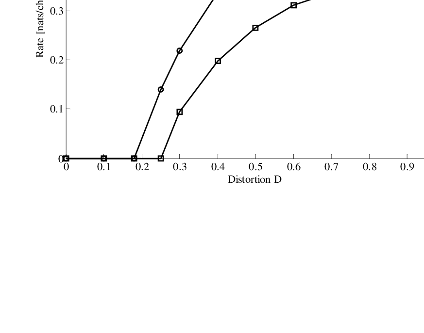
where $E[W(U-A)]=(\delta\gamma+\beta)\sigma_{W}^{2}$ $\textrm{and }E[(U-A)^{2}]=\delta{}^{2}P_{G}+(\delta\gamma+\beta)^{2}\sigma_{W}^{2}.$ The rate $I(U;Y)-I(U;S|A)$ optimized over parameters $(\alpha,\beta,\delta,\gamma)$ under the constraint (17) for different values of the distortion $D$ for $P_{A}=P_{X}=\sigma_{W}^{2}=\sigma_{Z}^{2}=1$ in Fig. (3). Moreover for reference, Fig. 3 shows also the rate achievable if distribution (12) is designed to be optimal for message transmission only as in [1, eq. (95)], and the rate achievable, if $A$ is selected to be independent of the message, namely, $\textrm{$\max$\ }I(U;Y|A)-I(U;S|A)$, where the mutual information terms are evaluated with respect to the joint Gaussian distribution given above in (16) under the constraint (17). The performance gains attainable by designing the transmission strategy jointly in the two phases and by accounting for the constraint (17) are apparent.

In this section the system model is detailed. The system is defined by the pmfs $p(x)$, $p(y_{1},y_{2}|x,$ $s,a)$, $p(s|a)$ and discrete alphabets $\mathcal{X},\mathcal{\textrm{ }A\mbox{,}\textrm{ }S\mbox{, and }Y}$ as follows. Given the messages $M_{1}$ and $M_{2}$, selected randomly from the sets $\mathcal{M}_{1}=[1,2^{nR_{1}}]$ and $\mathcal{M}_{2}=[1,2^{nR_{2}}]$, respectively, an action sequence $A^{n}\in\mathcal{A}^{n}$ is selected. As a result of this selection, the state sequence $S^{n}\in\mathcal{S}^{n}$ is generated as in the previous section. The action sequence $A^{n}$ and the input $X^{n}$ have to satisfy the average cost constraint (8). Given the transmitted signal $X^{n}=x^{n}$, the state sequence $S^{n}=s^{n}$, and the action sequence $A^{n}=a^{n}$, the received signals are distributed as $p(y_{1}^{n},y_{2}^{n}|x^{n},s^{n},a^{n})=\prod_{i=1}^{n}p(y_{1i},y_{2i}|x_{i},s_{i},a_{i})$. The decoders, based on the received signals $Y_{1}^{n}$ and $Y_{2}^{n}$ , estimate the messages $M_{1}$ and $M_{2},$ respectively.

We note that, given the definitions above, the distribution of the random variables $(M_{1},M_{2},A^{n},$ $S^{n},X^{n},Y_{1}^{n},Y_{2}^{n})$ factorizes as

where the arguments of the pmf range in the alphabets of the corresponding random variables.

Given a cost $\Gamma$, a rate pair $(R_{1},R_{2})$ is said to be achievable if, for any $\epsilon>0$ and sufficiently large $n$, there a exists a $(n,R_{1},R_{2},\Gamma,\epsilon)$ code. The capacity region $\mathcal{C}(\Gamma)$ is defined as the closure of all rate pairs $(R_{1},R_{2})$ that are achievable given the cost $\Gamma$.

In this section, a single-letter characterization of the capacity region is derived for the special case in which the channel is physically degraded in the sense that we have the condition

or equivalently we have that the Markov chain $(X_{i},S_{i},A_{i})-Y_{1i}-Y_{2i}$ holds for all $i\in[1,n]$.

The proof of achievability can be sketched as follows. The codewords $u_{2}^{n}(m_{2})$, encoding message $m_{2}\in[1,2^{nR_{2}}]$, are generated independently and i.i.d. according to the pmf $p(u_{2})$. Then, superimposed on each codeword $u_{2}^{n}(m_{2})$, $2^{nR_{1}}$ codewords $u_{1}^{n}(m_{1},m_{2})$ are generated independently according to the distribution $\prod_{i=1}^{n}p(u_{1i}|u_{2i}(m_{2}))$. To encode messages $(M_{1},M_{2})$, the action sequence $A^{n}$ is obtained as a deterministic function of $u_{1i}(M_{1},M_{2})$ and $u_{2i}(M_{2})$ such that $A_{i}=\textrm{$f_{a}$}(u_{1i}(M_{1},M_{2}),u_{2i}(M_{2}))$ for all $i\in[1,n]$. The transmitted symbol $X_{i}$ is obtained instead as a function of $u_{1i}(M_{1},M_{2})$, $u_{2i}(M_{2})$, and of the $i$th state symbol $S_{i}$ as $X_{i}=\textrm{$f_{x}$}(u_{1i}(M_{1},M_{2}),u_{2i}(M_{2}),S_{i})$. Decoder 2 decodes the codeword $u_{2}^{n}(m_{2})$, while decoder 1 decodes both codewords $u_{2}^{n}(m_{2})$ and $u_{1}^{n}(m_{1},m_{2})$. Using standard arguments, the rates (25) are easily shown to be achievable. The proof of the converse can be found in Appendix B.

In this section, we consider a special case of the model in Fig. 2 in which the action channel $p(s|a)$ is binary and given by

where the action $A$ is binary, $B\sim\textrm{Ber}(b)$ and the transmission channels are given by

where $Z_{1}\sim\textrm{Ber}(N_{1})$ and $\widetilde{Z}_{2}\sim\textrm{Ber}(\widetilde{N}_{2})$ are independent of each other and of $B$. We select the cost metric as $\gamma(a,x)=x$. We define $N_{2}=N_{1}*\widetilde{N}_{2}=N_{1}(1-\widetilde{N}_{2})+\widetilde{N}_{2}(1-N_{1})$.

As a first remark, consider the ideal system with $b=0$ (i.e., no interference) and no cost constraint (i.e., $\Gamma=\nicefrac{{1}}{{2}}$). The system reduces to a standard physical degraded binary symmetric broadcast channel, and thus the capacity region is given by the union over $\alpha\in[0,0.5]$ of the rate pairs satisfying the inequalities [12, p. 115]

We observe that, by construction, this rate region sets an outer bound on the rate achievable in the system at hand. The outer bound above is in fact achievable by setting $X=B$, $U_{2}\sim\textrm{Ber}(\nicefrac{{1}}{{2}})$, $U_{1}=U_{2}\oplus\widetilde{U}_{1}$ with $\widetilde{U}_{1}\sim\textrm{Ber}(\alpha)$, and $A=U_{1}$ in (25), where $U_{2}$ and $\widetilde{U}_{1}$ are independent. This entails that, by leveraging the actions, the interference-free capacity region (29) is obtained for all cost constraints $\Gamma\geq b$. It can be instead seen that, if one is forced to set $A$ to be constant, achieving the rate region (29) requires a cost $\Gamma=\nicefrac{{1}}{{2}}$, since $X$ needs to be distributed $\textrm{Ber}(\nicefrac{{1}}{{2}})$. This example illustrates the advantage of being able to affect the state via actions selected as a function of the messages.

In this section, we apply the setting of probing capacity introduced in [2] to the degraded broadcast channel. Following [2], the state sequence $S^{n}$ is thus assumed to be generated i.i.d. according to a pmf $p(s)$. Moreover, based on the messages $(M_{1},M_{2})$, the encoder selects an action sequence as in (18). However, here, through the choice of actions, the encoder affects the state information available at the encoder and the decoders, and not the state sequence $S^{n}$. Specifically, the encoder obtains partial state information $S_{e,i}=\textrm{$b_{e}$}(S_{i},A_{i})$, and the decoders obtain partial state informations $S_{d_{1,i}}=\textrm{$b_{d{}_{1}}$}(S_{i},A_{i})$ and $S_{d_{2,i}}=\textrm{$b_{d{}_{2}}$}(S_{d_{1,i}})$, respectively, where $i\in[1,n]$, and $b_{e}:\mathcal{S}\times\mathcal{A}\rightarrow\mathcal{S}_{e}$, $b_{d_{1}}:\mathcal{S}\times\mathcal{A}\rightarrow\mathcal{S}_{d_{1}}$ and $b_{d_{2}}:\mathcal{S}_{d_{1}}\rightarrow\mathcal{S}_{d_{2}}$ are deterministic functions for given alphabets $\mathcal{S}_{e}$, $\mathcal{S}_{d_{1}}$ and $\mathcal{S}_{d_{2}}$. Note that the state information available at decoder 2 is degraded with respect to that of decoder 1 (i.e., it is a function of the latter). As in [2], we assume that the state information at the encoder is characterized as

where $*$ represents the absence of channel state information at the encoder. Moreover, the state information $S_{e,i}$ is assumed to be available causally at the encoder so that the encoding function is $g_{2i}\textrm{: }\mathcal{M}_{1}\times\mathcal{M}_{2}\times\mathcal{S}_{e}^{i}\rightarrow\mathcal{X}$ (cf. (19)). The rest of the code definition is similar to Definition 4 with the caveat that the decoder 1 and 2 have available also the information sequences $S_{d_{1}}^{n}$ and $S_{d_{2}}^{n},$ respectively.

We note that, given the definitions above, the distribution of the random variables $(M_{1},M_{2},A^{n},$ $S^{n},X^{n},Y_{1}^{n},Y_{2}^{n})$ factorizes as

where the arguments of the pmf range in the alphabets of the corresponding random variables.

As discussed below, the setting at hand, which we refer to as having a probing encoder, is a special case of the one studied in Sec. II-A. Therefore, we can leverage Proposition 5 to obtain the following result.

References

- [1] T. Weissman, “Capacity of channels with action-dependent states,” IEEE Trans. Inform. Theory, vol. 56, no. 11, pp. 5396–5411, Nov. 2010.
- [2] H. Asnani, H. Permuter, and T. Weissman, “Probing capacity,” IEEE Trans. Inform. Theory, vol. 57, no. 11, pp. 7317–7332, Nov. 2011.
- [3] K. Kittichokechai, T. J. Oechtering, and M. Skoglund, “Coding with action-dependent side information and additional reconstruction requirements,” http://arxiv.org/abs/1202.1484, Feb 2012.
- [4] C. Choudhuri and U. Mitra, “Action dependent strictly causal state communication,” http://arxiv.org/abs/1202.0934, Feb. 2012.
- [5] Y. Steinberg, “Coding and common reconstruction,” IEEE Trans. Inform. Theory, vol. 55, no. 11, 2009.
- [6] Y.-H. Kim, A. Sutivong, and T. M. Cover, “State amplification,” IEEE Trans. Inform. Theory, vol. 54, no. 5, pp. 1850–1859, May 2008.
- [7] B. Ahmadi and O. Simeone, “On channels with action-dependent states,” http://arxiv.org/abs/1202.4438v1, Feb. 2012.
- [8] Y. Steinberg and T. Weissman, “The degraded broadcast channel with action-dependent states,” in Proc. IEEE Symp. Inform. Theory, Boston, USA, Jul. 2012.
- [9] Y. Steinberg, “Coding for the degraded broadcast channel with random parameters, with causal and noncausal side information,” IEEE Trans. Inform. Theory, vol. 51, no. 8, pp. 2867-2877, Aug. 2005.
- [10] S. Sigurjonsson and Y. H. Kim, “On multiple user channels with causal state information at the transmitters,” in Proc. IEEE Symp. Inform. Theory, Adelaide, Australia, pp. 72-76, Sept. 2005.
- [11] Y. Steinberg and S. Shamai, “Achievable rates for the broadcast channel with states known at the transmitter,” in Proc. IEEE Symp. Inform. Theory, Adelaide, Australia, pp. 2184 - 2188 , Sept. 2005.
- [12] A. El Gamal and Y. Kim, Network Information Theory, Cambridge University Press, Dec 2011.
- [13] G. Kramer, Topics in Multi-User Information Theory, Now Publishers, 2008.