Vacuum structure and string tension in Yang-Mills dimeron ensembles

Dimerons (or meron pairs) are those classical solutions of the Euclidean Yang-Mills equation which contain two meron centers where their only singularities are located [18]. In regular gauge, with the two merons located symmetrically at the distances $\pm a$ from the center at $x_{0}$, the SU$\left(2\right)$ dimeron solution family reads [18]

$$A_{\mu}^{\left(\text{D},\text{r}\right)}\left(x;\left\{x_{0},a,u\right\}\right)=\left[\frac{\left(x-x_{0}+a\right)_{\nu}}{\left(x-x_{0}+a\right)^{2}}+\frac{\left(x-x_{0}-a\right)_{\nu}}{\left(x-x_{0}-a\right)^{2}}\right]u^{\dagger}\sigma_{\mu\nu}u$$

(1)

where $\sigma_{\mu\nu}:=\eta_{a\mu\nu}\sigma_{a}/2$ with the Pauli matrices $\sigma_{a}$ and the ’t Hooft symbols $\eta_{a\mu\nu}$. (The latter are defined as $\eta_{a\mu\nu}=\varepsilon_{a\mu\nu}$, $\eta_{a\mu 4}=-\eta_{a4\mu}=\delta_{a\mu}$ for $\mu,\nu=1,2,3$ and $\eta_{a44}=0$ [39].) The unitary matrices $u$ are global SU$\left(2\right)$ color rotations. The dimerons (1) carry the same topological charge as instantons, i.e. $Q=1$. The anti-dimeron $\bar{A}_{\mu}^{\left(\text{D},\text{r}\right)}$ with opposite topological charge $Q=-1$ is obtained from Eq. (1) by replacing $\eta_{a\mu\nu}\rightarrow\bar{\eta}_{a\mu\nu}:=\left(-1\right)^{\delta_{\mu 4}+\delta_{\nu 4}}\eta_{a\mu\nu}$. In contrast to instantons, however, dimerons are not selfdual.

The solution class (1) depends on eleven real and continuous “collective coordinates” or “moduli” whose values uniquely and completely specify each member. Eight of these parameters, $x_{0,\mu}$ and $a_{\mu}$, determine the spacetime position and orientation of the dimeron while the remaining three determine the SU$\left(2\right)$ group elements $u$ ⁶⁶ 6 More generally, these are the $N_{c}^{2}-1$ “Euler angles” which parametrize (constant) SU$\left(N_{c}\right)$ group elements.. The collective coordinates correspond to those eleven independent combinations of the classical and continuous Yang-Mills symmetries, i.e. of Euclidean spacetime translations and rotations, conformal transformations and global SU$\left(2\right)$ color rotations, which transform a representative dimeron into a gauge-inequivalent solution [40].

It is instructive to consider several limits of the solution family (1). For $a\rightarrow 0$ the meron centers coalesce and the dimeron turns into a pointlike, regular-gauge instanton. (A finite-size instanton is reached after suitably regularizing the meron singularities, cf. Sec. II.3.) For $\left|a\right|\rightarrow\infty$, on the other hand, the dimeron breaks up into two merons. Although these merons maintain the fixed relative color orientation of Eq. (1), changing it by hand will yield increasingly action-degenerate two-meron solutions when the inter-meron separation $\left|a\right|$ becomes large. This is because the color-dependent attraction which locks the meron constituents of Eq. (1) into their rigid color orientation decreases with increasing $\left|a\right|$. Hence both instantons and merons are contained in the solution class (1) as limiting cases. The fields (1) therefore provide on-shell interpolations between instantons and isolated meron pairs, i.e. continuous paths in Yang-Mills solution space which connect these particular gauge fields. In our context these paths are of particular interest since they provide preferred doorways along which the dimerons may dissociate into merons. As already mentioned, such dissociation processes are conjectured to drive the deconfinement-confinement transition.

The solutions (1) have the same $\left|x\right|\rightarrow\infty$ behavior as an instanton in regular gauge [41, 35, 42], i.e. they contain a long-distance tail

$$A_{\mu}^{\left(\text{D},\text{r}\right)}\left(x\right)\overset{\left|x\right|\rightarrow\infty}{\longrightarrow}2\frac{x_{\rho}}{x^{2}}\sigma_{\mu\rho}$$

(2)

$\sim 1/\left|x\right|$ which implies an exceptionally weak localization. In multi-dimeron configurations these tails generate strong overlap interactions between the individual dimerons. Building dimeron ensembles by superposing solutions of the type (1) would thus lead to very strongly correlated systems, in some respects similar to the regular-gauge instanton ensembles studied in Ref. [14]. In the present work we will take a different route, however. In contrast to merons, dimerons – like instantons – may be transformed to singular gauges in which they are more strongly localized, with their long-range tails decaying as $1/\left|x\right|^{3}$. A superposition of singular-gauge dimerons thus improves the vacuum description at short distances, compared to superpositions of either regular-gauge instantons or single merons. As long as the characteristic dimeron size is small compared to the average inter-dimeron separation, furthermore, it will provide much better approximations to classical Yang-Mills solutions. This is essentially because at moderate pseudoparticle densities the contribution of the overlap regions to the action is much smaller than in regular-gauge dimeron superpositions. Hence singular-gauge multi-dimeron configurations provide a privileged testing ground especially for the semiclassical features of the CDG confinement mechanism [30, 24, 31].

In addition, dimeron configurations in singular gauge may also describe less classical or even fully quantum-mechanical aspects of confinement. This holds, in particular, for the vacuum disordering mechanism envisioned by CDG. The latter relies on the long-distance tails of the individual merons which come into play when the separation $\left|a\right|$ between the meron centers of the dimerons becomes large. As discussed above, the partner merons are then practically independent and regain their long-range tail $\sim 1/\left|x\right|$ (at least in isolation). The ensuing long-distance color correlations among these merons were found in Refs. [19, 14] to be far from semi-classical and to generate confinement. Of course, a complete dimeron dissociation into isolated and thus far separated merons is impossible in the finite spacetime volumes in which numerical simulations are feasible. (The same holds for the solution in which one of the merons delocalizes on the three-sphere at spacetime infinity [18, 24].) However, such isolated merons would anyhow be unphysical (since they carry infinite action) and incompatible with a finite dimeron density. Instead, one expects that beyond some typical separation the two meron centers of a dimeron experience stronger interactions with their individual field environment than with their partner. The rigid link between their color orientations can then be broken, i.e. the partner merons can become effectively independent of each other.

In order to construct the multi-dimeron configurations motivated above, we first transform the dimeron solution family (1) into a specific singular gauge,

$$A_{\mu}^{\left(\text{D},\text{s}\right)}=\hat{U}^{\dagger}\left(\hat{x}\right)A_{\mu}^{\left(\text{D},\text{r}\right)}\hat{U}\left(\hat{x}\right)+i\hat{U}^{\dagger}\left(\hat{x}\right)\partial_{\mu}\hat{U}\left(\hat{x}\right),$$

(3)

where $\hat{U}$ is the large, i.e. topologically active gauge group element

$$\hat{U}\left(\hat{x}\right)=i\hat{x}_{\mu}\sigma_{\mu}^{\left(+\right)}$$

(4)

($\sigma_{\mu}^{\left(+\right)}\equiv\left(\vec{\sigma},-i\right),$ $\hat{x}_{\mu}\equiv x_{\mu}/\sqrt{x_{\nu}x_{\nu}}$) which has a singularity at the origin of the coordinate system. The result can be cast into the form

$$A_{\mu}^{\left(\text{D},\text{s}\right)}=f_{1}\left(x,a\right)\text{ }x_{\nu}\bar{\sigma}_{\mu\nu}+f_{2}\left(x,a\right)\text{ }a_{\nu}X_{\mu\nu}\left(\hat{x}\right)$$

(5)

($\bar{\sigma}_{\mu\nu}:=\bar{\eta}_{a\mu\nu}\sigma_{a}/2$). Choosing for simplicity $x_{0}=0$ and $u=1$, the two scalar functions $f_{1,2}$ become

	$\displaystyle f_{1}\left(x,a\right)$	$\displaystyle:=\frac{2}{x^{2}}-\frac{1}{\left(x+a\right)^{2}}-\frac{1}{\left(x-a\right)^{2}},$		(6)
	$\displaystyle f_{2}\left(x,a\right)$	$\displaystyle:=\frac{1}{\left(x+a\right)^{2}}-\frac{1}{\left(x-a\right)^{2}}.$		(7)

The antisymmetric and anti-selfdual field $X_{\mu\nu}$ contains important parts of the SU$\left(2\right)$ and spacetime tensor structures (and their mutual couplings). Explicitly,

$$X_{\mu\nu}\left(\hat{x}\right)=\eta_{a\mu\nu}X_{a}\left(\hat{x}\right)\text{ \ \ \ with }X_{a}\left(\hat{x}\right)=\left(\frac{1}{2}-\hat{x}_{r}\hat{x}_{r}\right)\sigma_{a}+\hat{x}_{a}\hat{x}_{s}\sigma_{s}-\hat{x}_{4}\hat{x}_{s}\varepsilon_{asc}\sigma_{c}$$

(8)

(latin indices are spacial). After regularization of the short-distance singularity (cf. Sec. II.3) the $a\rightarrow 0$ limit turns the dimeron (5) into a singular-gauge instanton with $f_{1}\left(x,a=0\right)=2\rho^{2}/\left[x^{2}\left(x^{2}+\rho^{2}\right)\right]$ and $f_{2}\left(x,a=0\right)=0$. In the following, we will often refer with the term “dimeron” to both dimerons and anti-dimerons in singular gauge. Occasionally, we will use the term “pseudoparticle” for the same purpose.

The leading asymptotic behavior of the singular-gauge dimerons (5) is

$$A_{\mu}^{\left(\text{D},\text{s}\right)}\overset{\left|x\right|\gg\left|a\right|}{\longrightarrow}-4\frac{a_{\rho}x_{\rho}}{x^{4}}a_{\nu}\eta_{a\mu\nu}X_{a}\left(\hat{x}\right)\sim\frac{1}{x^{3}},$$

(9)

i.e. the long-range tail (2) has as intended disappeared and the overlap between neighboring dimerons is strongly reduced. (This is in contrast to the meron ensembles of Refs. [19, 14] whose constituents exist only in regular gauge.) In addition to the meron-center singularities at $x=\pm a$, the solution (5) inherits another singularity at $x=0$ from the gauge transformation (4). Hence the impact of the latter will disappear when forming (topologically insensitive) gauge-invariant quantities from Eq. (5). The regularization of these singularities will be discussed in Sec. II.3.

By construction, the singular-gauge dimerons (5) provide only a subset of the full solution family. The complete eleven-parameter family can be recovered by translating the solutions (5) to $x_{0}$ and by gauge-rotating them with a constant matrix $u\in$ SU$\left(2\right)$, i.e.

$$A_{\mu}\left(x;\left\{x_{0},a,u\right\}\right)=u^{\dagger}A_{\mu}^{\left(\text{D},\text{s}\right)}\left(x-x_{0}\right)u=R_{ab}\left(u\right)A_{\mu}^{\left(\text{D},\text{s}\right),b}\left(x-x_{0}\right)\frac{\sigma_{a}}{2}$$

(10)

where the orthogonal matrices $R_{ab}\left(u\right)=tr\left\{\sigma_{a}u^{\dagger}\sigma_{b}u\right\}/2$ are obtained from the condition $u^{\dagger}\sigma_{b}u=R_{ab}\left(u\right)\sigma_{a}$. The group elements $u$ depend on three real and continuous parameters which form (local) coordinates on the SU$\left(2\right)$ group manifold $S^{3}$. In the following it will be convenient to use the quaternion representation

$$u\left(c\right)=c_{0}+ic_{a}\sigma_{a}$$

(11)

which embeds $S^{3}$ into $R^{4}$ with Euclidean coordinates $c_{0},...,c_{3}$ by imposing the unit three-sphere constraint $\sum_{\alpha=0}^{3}c_{\alpha}^{2}=1$. In these coordinates $R$ takes the form

$$R_{ab}\left(u\left(c\right)\right)=\left(c_{0}^{2}-c_{c}c_{c}\right)\delta_{ab}+2c_{a}c_{b}-2\varepsilon_{abc}c_{0}c_{c}.$$

(12)

For our discussion below it will be useful to keep in mind that dimerons have three more continuous and noncompact collective coordinates than instantons (but three less than a pair of independent merons, due to the locking of the inter-meron color orientation). The three additional coordinates arise from the more complex structure of extended (i.e. $\left|a\right|\neq 0$) dimerons which requires more degrees of freedom to locate and orient them in spacetime. This results in a substantially larger “position entropy” [24, 43] which is instrumental in counterbalancing the (regularized) dimeron action which grows logarithmically with $\left|a\right|$. Indeed, the larger entropy is a necessary (but not sufficient) requirement for dimerons to dissociate with increasing coupling $g^{2}$ and to finally split up into their meron partners.

As motivated above, we intend to study a model which drastically reduces the field content of Yang-Mills theory (as integrated over in amplitudes and the partition function) to superpositions of $N_{D}$ dimerons and $N_{\bar{D}}\simeq$ $N_{D}$ antidimerons in singular gauge ⁷⁷ 7 It may be useful to recall that the superposition of singular-gauge dimerons is not gauge-equivalent to a superposition of regular-gauge dimerons., i.e.

$$A_{\mu}\left(x,\left\{C_{I,i},\bar{C}_{\bar{I},i}\right\}\right)=\sum_{I}^{N_{D}}A_{\mu}^{\left(\text{D},\text{s}\right)}\left(x;\left\{C_{I,i}\right\}\right)+\sum_{\bar{I}}^{N_{\bar{D}}}\bar{A}_{\mu}^{\left(\text{D},\text{s}\right)}\left(x;\left\{\bar{C}_{\bar{I},i}\right\}\right)$$

(13)

with $N\equiv$ $N_{D}+N_{\bar{D}}$. Each term in this sum is uniquely characterized by the set $\left\{C_{I}\right\}=\left\{x_{0,I},a_{I},c_{I}\right\}$ of collective coordinates of the corresponding (anti-) dimeron. We recall that the configurations (13) differ distinctly from those obtained by transforming a regular-gauge dimeron superposition into (any) singular gauge. This is because in Eq. (13) the gauge of each dimeron is chosen relative to its individual position. One may wonder, incidentally, whether $n$-meron solutions with $Q>1$ and their anti-solutions should be added to the superposition ansatz (13). As in the case of instantons, however, the Bogomoln’yi-type bound $S\geq\left(8\pi^{2}/g^{2}\right)\left|Q\right|$ on the action [41] implies that such multi-(anti)-meron contributions to the partition function are exponentially suppressed relative to the dimeron contributions ⁸⁸ 8 From the practical point of view this is fortunate since no multi-meron solutions with $\left|Q\right|>1$ seem to be known analytically.. Since the entropy increases only logarithmically with $n$ and thus cannot compensate this suppression, such multi-meron contributions may be safely neglected.

Nevertheless, the ansatz (13) should be regarded as a rather minimal choice. It is mainly geared towards a transparent study of the proposed (instanton and) dimeron dissociation mechanism and its role in the deconfinement-confinement transition [30, 24, 31]. Hence there are several natural directions in which Eq. (13) may be extended in future studies to provide a more complete description of the Yang-Mills vacuum physics. An example would be to add the meron-antimeron pair solutions [18] of the Yang-Mills equations, again individually transformed into singular gauge. This would maintain the approximately semiclassical nature of the configurations at small $\left|a\right|$ and yield a richer dynamics. However, it would probably also lead to a less transparent interpretation of the results, and we do not expect the topologically trivial meron-antimeron pair configurations to provide qualitatively new insights into the transition behavior. Indeed, their limits for $\left|a\right|\rightarrow 0$, a pure-gauge field of zero action, and for $\left|a\right|\rightarrow\infty$, a meron and an independent antimeron, indicate that meron-antimeron pairs do not generate new pathways for the transition. More promising improvement options would include generalizations of the dimeron superposition ansatz (13) which allow for a complete transition into a meron ensemble (e.g. by releasing the rigid color locking between the dimerons’ meron partners beyond a suitable intermeron separation $\left|a\right|_{\min}$) or the admixture of a pure instanton component [24, 31] with a realistic size distribution [44].

As discussed above, we view the dimeron configurations (13) as a pertinent subset of the SU$\left(2\right)$ gauge fields governed by the Yang-Mills dynamics. Hence we define the partition function of our dimeron model as

$$Z=\int\mathop{\displaystyle\prod}\limits_{I,\bar{I}}^{N_{D},N_{\bar{D}}}dC_{I}d\bar{C}_{\bar{I}}\exp\left\{-S\left[A_{\mu}\left(\left\{C_{I,i},\bar{C}_{\bar{I},j}\right\}\right)\right]\right\}$$

(14)

where $S$ is the Euclidean Yang-Mills action

$$S\left[A\right]=\frac{1}{2g^{2}}\int d^{4}xtr\left\{F_{\mu\nu}F_{\mu\nu}\right\}=:\int d^{4}xs\left(x\right)$$

(15)

and $F_{\mu\nu}$ is the gauge field strength

$$F_{\mu\nu}\left(x\right)=\partial_{\mu}A_{\nu}\left(x\right)-\partial_{\nu}A_{\mu}\left(x\right)-i\left[A_{\mu}\left(x\right),A_{\nu}\left(x\right)\right].$$

(16)

As already indicated, we expect the gauge interactions among the dimerons in Eq. (14) to play an important role in generating confining long-range correlations for large $\left|a\right|$ and, in particular, to provide a disordering mechanism for the vacuum. This is in contrast to the situation in non-confining singular-gauge instanton ensembles where for most amplitudes a random orientation of the instantons (i.e. the neglect of the interaction term $\exp\left(-S\right)$ in Eq. (14)) yields a reasonable approximation to the vacuum physics [23].

The integration over the collective coordinates will be performed with the measure

$$dC=d^{4}x_{0}d^{4}ad\mu\left(\vec{c}\right)$$

(17)

($d\mu\left(\vec{c}\right)$ is the SU$\left(2\right)$ Haar measure) for the dimerons, and analogously for the anti-dimerons. This type of measure if familiar from instanton vacuum models [23]. An improved alternative may include Jacobians which arise from the transformation of the linear gauge-field measure $dA$ into the collective-coordinate basis and thereby implement the full moduli-space metric. Finally, an additional $a$ dependence of the measure can emerge from the trace anomaly [24, 31].

The singular-gauge dimeron solutions (5) contain two types of singularities. The first are those located at the constituent meron centers $x=x_{0}\pm a$ which persist in any gauge. In addition, there is a gauge singularity inherited from the topologically large and thus necessarily singular gauge transformation (4), chosen to sit at the origin. In isolated dimerons, such gauge singularities could be gauged away and would therefore not affect (topologically insensitive) observables. This ceases to be the case for the superpositions (13), however, where the location of the gauge singularities varies with the positions of the pseudoparticles.

Since both types of singularities would impede our numerical simulations, they have to be regularized in a physically acceptable manner. (Recall that the individual dimeron fields (1) and (5) do not solve the Yang-Mills equation at their singularities, so that a suitably localized regulator will only minimally affect the semiclassical properties of the configurations (13).) A natural way to regularize the singularities at the meron centers is to add the square of a “size” parameter $\rho$ to the denominators $\left(x-x_{0}\pm a\right)^{2}$ in Eqs. (6) and (7). Such a regulator imitates the way in which the size parameter enters the instanton solutions. Hence it may arise from scale-symmetry breaking quantum fluctuations which are expected to smear the classical singularities. A finite $\rho$ furthermore acts as a UV cutoff since it limits the gradients of the configurations (13). Of course, the regularized field configurations cease to be exact solutions of the classical Yang-Mills equation. Hence the value of $\rho$ should be chosen large enough to avoid sizeable discretization errors (cf. Sec. III.4) but also small enough to avoid unnessary deformations of the dimeron solutions from the semiclassical saddle points. We have found $\rho^{2}=0.3$ to be a reasonable compromise between both criteria and will use this value in our numerical simulations, if not stated otherwise.

The remaining singularities are, at least for isolated dimerons, gauge artefacts. They remain unlikely to have a physical impact in our dimeron superpositions, too, but they may nevertheless cause problems in numerical approximations (even for single dimerons), e.g. when subtle cancellations in gauge-invariant quantities are upset by discretization errors. A finite-size regulator as above would hardly help to avoid such problems since it would just spread out the unphysical action-density peaks at the singularities. Hence we treat these gauge-dependent singularities in a pragmatic way, namely by interpolating the gauge field in 4$d$ balls of radius $\varepsilon$ around the singularities with the field value at a specific point on the surface of the ball. In practice, it turns out that with $\rho^{2}=0.3$ these highly localized singularities are smoothly regularized by taking $\varepsilon$ as small as $\varepsilon=5\times 10^{-10}$. (The values of dimensionful quantities, such as $\rho$ and $\varepsilon$ above, are given in “numerical units” originating from the discretization grid to be introduced in Sec. III.1. As a convenient length unit we have chosen $a=0.1$, i.e. a tenth of the distance between nearest grid points. (Of course, this $a$ should not be confused with the four-vector $a$ which parametrizes the dimeron solutions.) When transforming our results into physical units starting from Sec. IV.3, we will denote quantities in these numerical units by a hat above their symbols, cf. Sec. IV.3.) In our simulations it typically took several hundred sweeps through configurations of $N=487$ pseudoparticles (cf. Sec. III.2) before such a singularity was first encountered. (Even with a dramatically reduced floating-point variable length of 16 bits, incidentally, we have observed no overflows (which unregularized gauge singularities would generate) when evaluating the action density of a regularized two-dimeron configuration.)

Owing to the translational invariance of the Yang-Mills dynamics (15), ensemble averages over the pseudoparticle configurations (13) in infinite spacetime will likewise be translationally invariant. In our simulations we are restricted to a bounded volume of numerically manageable size, on the other hand, and thus have to keep boundary artefacts in calculated amplitudes under control, ideally within the size of the statistical uncertainties. Our initial step in this direction was to adopt singular-gauge dimerons with their more rapidly decaying long-range tails as the constituents of our gauge-field configurations (13). A sufficient suppression of boundary artefacts turned out to require additional measures, however, since the overlap among the still rather moderately localized dimerons generate important (and typically repulsive) interactions over ranges beyond the average nearest-neighbor distance. In fact, these interactions are expected to play an important role in the confinement mechanism and should thus be distorted as little as possible by the boundary. Simulation costs, on the other hand, with their by far largest part due to integrating the action density on a spacetime grid, should be kept minimal.

In order to approximately meet these conflicting goals, we will adopt a multi-layered description of the boundary with decreasing grid-point density towards the outer layers, as sketched in Fig. 1. The innermost “core volume” is a rectangular spacetime box in which we intend to evaluate amplitudes and thus require the physics to best approximate the infinite-volume limit. In order to allow for an efficient evaluation of Wilson loops with elongated time directions in Sec. IV.6, this volume and its grid are chosen to be asymmetric. One dimension, singled out as the Euclidean time direction, contains 40 grid points while each spacial dimension contains 25. This turns out to provide a sufficiently high resolution for the amplitudes to be calculated below (cf. Sec. III.4).

The core volume is encompassed by an “ensemble volume” which contains the (anti-) meron centers of all (anti-) dimerons. Its surface is implemented numerically by rejecting Metropolis updates (cf. Sec. III.2) during which a meron center would leave this volume. The extent of the ensemble volume in a given direction will be taken 15% larger than that of the core in the same direction. In the part of the ensemble box which surrounds the core we reduce the grid-point density to $\left(2/3\right)^{4}\sim 20\%$ of that in the core volume. This turns out to yield a still adequate resolution while substantially reducing the computational cost of evaluating the action.

A satisfactory suppression of field distortions inside the core volume turns out to require an additional precautionary measure, however. It consists in correcting for a particularly prominent boundary effect, namely the artificial attraction of the pseudoparticles to the surface of the ensemble volume. The latter arises because a substantial part of the action density of dimerons near the boundary is located outside the ensemble volume and thus not accounted for while the compensating tails of outside dimerons reaching into the ensemble volume are neglected. We approximately remove this artefact by surrounding the ensemble box with another, “covering” volume which extends beyond the ensemble box by 10% of the core size in each direction. To keep the additional computational costs under control, we decrease the grid-point density of the outermost shell (i.e. the part of the covering volume not shared by the ensemble volume) inversely with the distance from the ensemble boundary. Since this shell does not contain the rapidly varying fields close to the meron centers, calculating the action in the full covering volume indeed largely prevents the fake attraction to the ensemble boundary (cf. Sec. IV.2). Alternatively, finite-size effects in pseudoparticle ensembles can be efficiently corrected by employing the Ewald summation technique, as has been shown very recently in the simpler case of Abelian dyon field ensembles [28].

We evaluate the discretized functional integral over the pseudoparticle fields, i.e. the multi-dimensional integral over their collective coordinates in the partition function (14) or any other amplitude, stochastically by Monte-Carlo importance sampling. Hence we average over dimeron configurations chosen randomly from a Gibbs distribution with Boltzmann factor $\exp\left(-S\right)$ where $S$ is the Yang-Mills action (15). More specifically, we use the Metropolis algorithm to generate homogeneous Markov sequences of dimeron configurations that visit fields with larger probabilities more often. After reaching equilibrium, the probability of finding a configuration in the ensemble of subsequently generated fields follows the Gibbs distribution.

The initial pseudoparticle configurations for these Markov sequences are obtained by choosing their collective coordinates from a uniform random distribution. This procedure has equal access to all members of the configuration space and practically always results in configurations far from equilibrium, with actions several orders of magnitude above their equilibrium values. We have also tested various more ordered initial arrangements of the dimerons and convinced ourselves that those lead within errors to equivalent equilibrium ensembles (see Sec. III.4).

For the Markov update of the $n$-th configuration $A_{n}$ to its sequel $A_{n+1}$ according to the Metropolis rules, we first generate some candidate configuration $A^{\prime}$ by randomly choosing an individual pseudoparticle in $A_{n}$ and modifying alternately (from one candidate to the next) either its position, i.e. $a_{\mu}\rightarrow a_{\mu}+da_{\mu}$ and $x_{0,\mu}\rightarrow x_{0,\mu}+dx_{0,\mu}$, or its color orientation $c_{i}\rightarrow c_{i}+d\mu\left(c_{i}\right)$. The increments $da,$ $dx_{0}$ and $dc$ are chosen randomly and uniformly subject to the constraint that their length remains limited. More specifically, we demand $\left|dx_{0}\right|\in\left[0,\left|dx_{0}\right|_{\text{max}}\right]$, $\left|da\right|\in\left[0,\left|da\right|_{\text{max}}\right]$ as well as $\left|dc\right|\in\left[0,\left|dc\right|_{\text{max}}\right]$ ⁹⁹ 9 More precisely, all four coefficients of the quaternion representation (11) are varied independently. The constraint among them is reinstated only afterwards by rescaling all coefficients with a common factor. (Hence $d{\mu}\left(c_{i}\right)$ represents the Haar measure on SU$\left(2\right)\sim S^{3}$.) and further restrict $\left|da\right|_{\text{max}}=\left|dx_{0}\right|_{\text{max}}$. The candidate configuration $A^{\prime}$ is accepted as the new configuration $A_{n+1}$ with probability $\min\left\{1,\exp\left(S\left[A\right]-S\left[A^{\prime}\right]\right)\right\}$. If a candidate is rejected, the unchanged configuration is taken as $A_{n+1}$ (and included in measurements like all others).

The choice of the maximal modification step sizes $\left|da\right|_{\text{max}}$ and $\left|dc\right|_{\text{max}}$ can be used to optimize both the thermalization rate and the decorrelation among subsequent field configurations of the generated ensembles. This requires a compromise between too small values, which impede the progression through configuration space, and too large values which more strongly decorrelate subsequent configurations but cause an unefficiently large update rejection rate. Examination of the relation between maximal step sizes and typical acceptance probabilities suggests an optimal acceptance rate of about 25% for updates in both position and color space. During the initial thermalization process we will therefore increase (decrease) the maximal step sizes $\left|da\right|_{\text{max}}$ and $\left|dc\right|_{\text{max}}$ after every 10 consecutive candidate field configurations by 10% if the average acceptance rate for these configurations falls below (rises above) 25%.

This dynamical step-size adaptation procedure accelerates the approach to equilibrium and avoids getting trapped into approximate would-be equilibria. Initially, i.e. far from equilibrium and near the high-action random configurations, the fields can relax in larger steps while closer to equilibrium the action fluctuations become smaller and require decreasing step sizes to maintain sufficient acceptance rates. From the time when approximate equilibration sets in, however, the step size is kept constant to preserve detailed balance. We further note that increasing $g$ increases the acceptance probability since the Yang-Mills action (15) scales as $g^{-2}$. Hence larger $g$ allow for larger step sizes, accelerate thermalization (in less Markov steps) by decreasing the autocorrelation time and result in equilibrium ensembles with larger entropy.

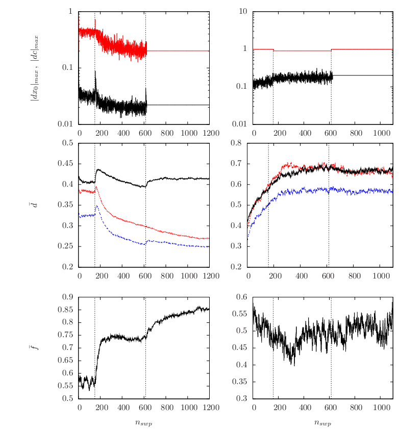
As a case in point, for $g^{2}=1$ (and $\rho^{2}=0.3$) we find $\left|da\right|_{\text{max}}\sim 0.05$ and $\left|dc\right|_{\text{max}}\sim 0.1$ in equilibrium, where the scale of the fluctuations is set by the competition between action and entropy. (For $\rho^{2}=0.2$, i.e. for more strongly localized meron centers, one instead reads off the smaller values $\left|da\right|_{\text{max}}\sim 0.025$ and $\left|dc\right|_{\text{max}}\sim 0.2$ from Fig. 2.) For $g^{2}=10^{2}$, on the other hand, one finds the indeed substantially larger maximal step sizes $\left|da\right|_{\text{max}}\sim\left|dc\right|_{\text{max}}\sim 0.5$ (again for $\rho^{2}=0.3$). The decreasing step width during a typical thermalization history is plotted in the uppermost row of Fig. 2 for $g^{2}=1$ and $g^{2}=25$. Note that different step sizes in position and color space are generally required to obtain action changes of comparable magnitude.

The efficiency of the ensemble generation process can be further improved by exploiting the during equilibration decreasing ruggedness and action of the dimeron configurations in yet another way, namely by starting on coarser grids and increasing the resolution only when a higher accuracy of the action evaluation becomes necessary. Indeed, as long as the action density is comparable to or larger than its value around the regularized meron centers, a reduced resolution is generally sufficient and can save computer time. During thermalization the overall action decreases strongly, however, and the grid must be refined to prevent the then more prominent meron centers from artificially reducing their action density by “hiding” between grid points. In practice, we implement this refinement procedure by starting the simulations with a $\left(1/3\right)^{4}$ times smaller grid-point density. When the values of suitable quantities (e.g. the distance between nearest-neighbor meron centers) begin to saturate, this factor is increased to $\left(2/3\right)^{4}$. Only after again reaching approximate saturation the full grid-point density of Sec. III.1 is activated for the final approach to equilibrium and the subsequent generation of the thermal ensembles. The approximate saturation plateaus and subsequent grid refinements (indicated by dotted vertical lines) are clearly visible in the thermalization histories of Fig. 2.

In the following we will denote a set of $2N$ consecutive Markov steps as a “sweep” (where $N=N_{D}+N_{\overline{D}}$, cf. Sec. II.2). During such sweeps each pseudoparticle of a configuration is on average once considered for a full update. (The factor two arises since the individual Markov steps attempt to modify either a dimeron’s position or its color orientation, i.e. only one of the two subsets of its degrees of freedom.) After four consecutive sweeps with the acceptance rate kept fixed at $1/4$, all pseudoparticles in a configuration are therefore on average updated once. In order to reduce autocorrelations among ensemble configurations and thus to increase the statistical independence of successive measurements, we will only select the configurations generated by every fifth sweep (after approximate equilibration of the Markov chain) as ensemble members and employ a binning procedure to calculate amplitudes and their errors (cf. Sec. III.5).

As indicated in the previous section, a reliable calculation of vacuum expectation values as ensemble averages requires a sufficient thermalization of the Markov sequences which generate the ensemble configurations. Our criteria for when their distribution approximates the equilibrium distribution closely enough are based on the measurement of several observables and correlations to be described below.

First insights into the configurations’ thermalization properties can be gained by following the Markov evolution of the average distance $\bar{d}$ of a fixed meron center to its nearest neighbor as a function of the number of sweeps. Two examples for such histories are depicted in the second row of Fig. 2. In the left panel the coupling is set to $g=1$, i.e. our smallest value, which results in the slowest equilibration rates we have to deal with in this paper (cf. Sec. III.2). (For these measurements we have also selected a smaller meron-size regulator $\rho^{2}=0.2$ which further slows the equilibration process.) A first and general insight to be read off from this figure is how the degree of thermalization reached after a given number of sweeps depends on the measured quantity. While the average distance to the closest neighboring meron of equal topological charge appears to have equilibrated after about 800 sweeps, the analogous distance for oppositely charged merons may not be fully thermalized even after 1200 sweeps. A similarly long equilibration history can be observed for the average probability $\bar{f}$ that the nearest neighbor of a given meron center has opposite topological charge, as plotted in the last row of Fig. 2. This behavior seems to indicate that the average distance between two meron centers from the same dimeron equilibrates faster than their average separation from the meron centers of neighboring dimerons. For $g^{2}=25$ the typical relaxation times reduce to at least half of those at $g^{2}=1$, confirming the expectation that more strongly coupled ensembles thermalize faster.

For a better understanding of the global thermalization behavior, and especially of the character and uniqueness of the reached equilibria, we have also compared ensembles resulting from different initial configurations. More specifically, we have prepared a set of initial dimeron arrangements in which the pseudoparticles were regularly positioned at maximal average distances. Their topological charges, color orientations and sizes were chosen either to approximate different types of action minima or to imitate close-to-equilibrium configurations found in previous thermalization runs.

All ensembles resulting from these different initializations turned out to generate within errors the same averages. This provides, for once, evidence for the ergodicity of the underlying Markov process, i.e. for its ability to access any possible dimeron configuration in a finite number of steps. More importantly, this result strongly supports the conclusion that the thermalization processes indeed have come sufficiently close to equilibrium, i.e. that our measurements in Sec. IV are performed in almost thermalized ensembles. This conclusion is strengthened by the fact that all our runs with non-random initializations were performed at $g^{2}=1$ where equilibration is particularly slow.

We now turn to the analysis of the systematic errors which arise from finite-resolution and finite-size effects. We then describe the steps taken to control them by accordingly refining our calculational strategy. Additional error-reduction measures, which apply to the calculation of specific amplitudes only, will be outlined in their corresponding sections below.

Discretization errors arise in our context from the practical necessity to sample the field configurations (13) on spacetime grids of finite resolution. To meet our accuracy requirements, we adapt the grid-point density according to the characteristic length and gradient scales in the pseudoparticle configurations under consideration. During thermalization, where these scales change drastically, we do so dynamically as described in Sec. III.2. In the (approximately) thermalized ensembles, on the other hand, these scales are essentially fixed by the pseudoparticle density and by the size of the regularized meron-center singularities ¹⁰¹⁰ 10 The singular-gauge induced singularities are so strongly localized (even after regularization, cf. Sec. II.3), on the other hand, that they have practically no impact on the simulations.. As described in Sec. II.3, the regulator is chosen about five times larger than the lattice unit $a=0.1$, at $\rho\simeq\allowbreak 0.55$. This proves sufficient to keep the action of an isolated dimeron practically independent of its position on the grid. Although configurations with gradients larger than those around single meron centers frequently occur among the dimeron superpositions (13), their enhanced action renders them relatively unimportant when thermalization is achieved. This explains why we did not encounter such configurations in our equilibrated ensembles (cf. Sec. IV.2).

The grid resolution’s impact on the calculated action values and on the thermalization process can be seen directly in the Markov evolution histories of Fig. 2. The two vertical lines indicate the sweep numbers at which the resolution of the grid is refined (cf. Sec. III.2). The full resolution, corresponding to $a=0.1$, is reached only after the second refinement step. In order to provide a particularly stringent test of discretization errors, we have reduced our regulator $\rho$ for this simulation by a factor of four, to $\rho=0.14$. This size is of the order of the minimal lattice unit and about half of the value $\rho\sim 0.3$ below which discretization errors become a concern. As a consequence, one observes that the evolution of both plotted quantities (i.e. the average meron-center distances $\left\langle d_{\text{nearestMM}}\right\rangle$ and the probability for the nearest neighbor-meron to have opposite $Q=\pm 1/2$) on the coarsest grid begins to saturate at a preliminary would-be equilibrium when further relaxation is prevented by insufficient action-density resolution. Already after the first grid refinement, however, relaxation continues until the deviation from the thermal values reduces to about 15 – 20%. The equilibrium values are approached after the second refinement step. For our standard meron size $\rho\simeq 0.55$ the discretization errors will of course be much smaller and should be well under control. This conclusion is confirmed by checks on other observables, e.g. when calculating link elements and their concatenations into Wilson loops in Sec. IV.6.

We now turn to the discussion of finite-size effects. Those are artefacts of the simulation volume’s boundary and turn out to be more difficult to control than the discretization errors. Our choice of the more strongly localized dimerons in singular gauge (5) as the constituents of the configurations (13) was partly motivated by reducing such boundary effects. For the same purpose we designed the multi-layered boundary outlined in Sec. III.1. Nevertheless, sizeable boundary artefacts of different origins, of different $g^{2}$ dependence and with varying impact on the calculated quantities remain to be dealt with. In order to analyze those quantitatively, we start by monitoring violations of translational invariance in the ensemble-averaged action density $\left\langle s\left(x\right)\right\rangle$ as a function of the distance from the boundary for two values of $g^{2}$. The results are of direct physical and practical importance since $\left\langle s\right\rangle$ is related to the gluon condensate and since a reliable evaluation of the action is indispensable for generating trustworthy ensembles.

The action density $s\left(x\right)$, as defined in Eq. (15), can be obtained analytically by inserting the dimeron superposition (13) into the field strength (16). The ensemble average $\left\langle s\right\rangle$ is then evaluated as outlined in Sec. III.2, with ensemble configurations taken from every fifth sweep after equilibration. In order to visualize the local homogeneity properties of the action density in different sectors of the simulation volume, we plot $\left\langle s\right\rangle$ in Figs. 3 and 4 as a function of the distance from the center of the box along two different directions. The latter were chosen to provide insight into the anisotropy of the boundary effects, caused in particular by our asymmetric grid with its elongated temporal direction. (Instead of calculating the values of $s\left(x\right)$ at neighboring, equidistant points throughout these directions, we surround them with adjacent hypercubic boxes of side length $0.2$ inside which we sample $s\left(x\right)$ at 10 randomly chosen points.)

We start our discussion of the $\left\langle s\right\rangle$ plots with those generated at our smallest coupling value, $g^{2}=1$. In the left panel of Fig. 3 we show $\left\langle s\right\rangle$ (black squares, full line) along the time direction, in the right panel along the average over all diagonals of the spacial box at the mid point of the time axis. Deviations from a translationally invariant, i.e. constant $\left\langle s\right\rangle$ near the center of the box are somewhat smaller along the time direction than along the diagonal. This is expected since the former keeps a larger distance from the spacial boundaries. Nonetheless, $\left\langle s\right\rangle$ fluctuates considerably even in the temporal direction and even close to the box center. A reasonable fit to a constant plateau remains possible inside most error bars up to distances of order $1.0$ both along the time and diagonal directions, however, as also shown in Fig. 3. Beyond distances of about ten lattice units the missing field contributions from outside of the box volume (cf. Sec. III.1) begin to reduce the action density substantially.

As a consequence of these results, we will restrict the volume in which we evaluate amplitudes to subvolumes of the core box in which the maximal distances from the center are of order one (if not noted otherwise). To demonstrate the $g^{2}$ dependence of the boundary effects, we further show the two analogous $\left\langle s\right\rangle$ profiles for $g^{2}=25$ in Fig. 4. Clearly, the boundary effects are strongly reduced and the regions close to the center now show manifest plateaus which extend up to distances $\sim 1.5$ from the center. With further increasing $g^{2}$ the boundary artefacts become even more restricted to the surface region until the growing dimeron dissociation (i.e. the growing intermeron distance $2\left|a\right|$) creates a different type of sensitivity to the boundary, as discussed in Secs. III.1 and IV.2.

Since in general both character and strength of the boundary artefacts are amplitude dependent, we have also monitored the vacuum expectation value of quadratic “probe” Wilson loops $W$ as a function of their distance from the box center. The results will guide us in reliably calculating the expectation values of rectangular Wilson loops in Sec. IV.6. Since the largest among these loops play a crucial role in understanding the confinement properties of dimeron ensembles, it becomes especially important to understand the boundary’s impact on them. We survey it by evaluating the expectation values $\left\langle W\right\rangle$ of quadratic Wilson loops (for details see Sec. IV.6) of side length $0.5$ centered along the same two lines as the action density $\left\langle s\right\rangle$ above. The loop orientation turns out to have no significant impact on the value of $\left\langle W\right\rangle$ and will thus be averaged over. In Fig. 3 we have included plots of $450\times\left\langle W\right\rangle$ along the time direction in the left panel and along the average over the spacial diagonals in the right panel for $g^{2}=1$, and in Fig. 4 we display $20\times\left\langle W\right\rangle$ for $g^{2}=25$. In all four cases, with growing $t,r$ the distance dependence of $\left\langle W\right\rangle$ becomes increasingly proportional to that of the average action density $\left\langle s\right\rangle$. For quadratic Wilson loops of minimal size this is expected since such “plaquettes” form the essential part of a discrete approximation to the Yang-Mills action density. In our case, the observed proportionality further indicates that the configurations are sufficiently smooth over our rather large test loops, probably because their side length is comparable to the regulated meron size $\rho\simeq 0.55$.

To summarize, while discretization errors in our dimeron simulations can be reliably controlled, we have observed significant violations of translational invariance in both action density and Wilson loops. Although our efforts to reduce boundary artefacts prove effective close to the center of the core box, substantial deviations from homogeneity set in at distances of order one, in particular for our smallest coupling value $g=1$ where they are most pronounced. These boundary effects originate from a combination of the strong intermediate-range interactions between dimerons and the collective effects emanating from the boundary (cf. Sec. III.1). The lessons learned from the above analysis will guide us in keeping boundary artefacts of our results tolerably small, mainly by relying on specifically reduced volumes in which to evaluate amplitudes.

The effective dimeron field theory introduced in Sec. II has three adjustable parameters: the gauge coupling $g^{2}$, the meron-center size $\rho$, and the approximately equal numbers $N_{D}\simeq N_{\overline{D}}$ of dimerons and antidimerons. We have generated all our ensembles with $N=N_{D}+N_{\overline{D}}=487$ pseudoparticles, divided into $N_{D}=243\simeq N/2$ dimerons and $N_{\overline{D}}=244\simeq N/2$ antidimerons, in the multi-layered multi-grid volume specified in Sec. III.1. The meron centers are smeared as described in Sec. II.3, with a common regulator value $\rho^{2}=0.3$. We have generated two independent ensembles for each of the coupling values $g^{2}\in\left\{1,25,100,1000,\infty\right\}$ (with decreasing number of members) and a third one for $g^{2}=1$. The total number of sweeps per coupling in equilibrium as well as the maximal stepsizes are collected in Tab. 1

In order to estimate autocorrelation effects in the ensembles with $g^{2}=1$, where they should be maximal, we have calculated autocorrelation functions for several quantities of interest, including the average distance between nearest-neighbor meron centers of equal and opposite topological charges. For those of opposite topological charge the autocorrelations decay fastest, after about 300 – 400 equilibrium sweeps, while this takes up to a few hundered sweps longer for equally charged neighbors. The autocorrelation functions for the average distance between nearest-neighbor dimerons, on the other hand, show no obvious preference for either equally or oppositely charged neighbors. Both distances approximately decorrelate after 500 sweeps. The same holds for the average distance between the dimerons’ meron partners.

Based on the above observations, we have adopted the following strategy to reduce autocorrelations. The ensembles contain the configurations generated by every fifth Metropolis sweep. The total number of equilibrium sweeps (per coupling) is divided into ten bins. (For $g^{2}=1$ a bin thus contains about $180$ sweeps and about $36$ ensemble configurations.) The quantities of interest are then calculated on every ensemble configuration, and their mean values are obtained for each bin. Finally, the ensemble average is computed as the mean value of the bin averages, and its error is estimated as the standard deviation among the bin averages (if not noted otherwise). (On an Intel Core 2 Quad Q6700 processor at 2.67 Ghz a thermal Markov step takes about $t_{m}\sim 7$ seconds and a thermal sweep $2Nt_{m}\sim\allowbreak 1.\,\allowbreak 89$ hours.)

One of the essential features of the CDG mechanism is that with increasing coupling instantons are supposed to gradually dissociate into dimerons and to finally break up into their two meron partners. This process is suggested to be driven by a competition between the attraction among the regularized meron centers and their position entropy which increases with $g^{2}$ (since the latter plays the role of temperature in the classical statistical analog ensemble). The competition is effective because both energy and entropy depend logarithmically on the distance $2\left|a\right|$ between the meron centers. In fact, this distance will play a key role in characterizing both the structure of the ensembles’ dimeron constituents and the interactions among them. The latter depend sensitively on the dimerons’ color dipole moment which is of $O\left(a^{2}\right)$.

Before the dimerons break up completely, they should already have effectively released their two meron centers which then become the dynamically active degrees of freedom. In fact, this is expected to signal the onset of a phase transition in a finite system like ours where a complete $\left|a\right|\rightarrow\infty$ dissociation is prevented by the boundary. With their slowly decaying and thus strongly overlapping long-distance tails ($\sim 1/x$) the essentially independent merons may then sufficiently disorder the vacuum to generate linear quark confinement. In the above sense, our dimeron configurations thus approach confining meron ensembles of the type studied in Refs. [14, 19]. One should keep in mind, however, that our dimeron superposition ansatz (13) is not rich enough to describe ensembles of completely independent merons since it does not allow to untie the rigid color locking between the meron partners.

Guided by the above considerations we are thus led to study the coupling dependence of the average dimeron dissociation $2\left\langle\left|a\right|\right\rangle$ in our ensembles. These average inter-meron distances, which contribute to the typical dimeron size scale $\sim 2\left(\rho+\left\langle\left|a\right|\right\rangle\right)$, are plotted as a function of the square coupling $g^{2}$ in Fig. 5 and listed in Table 2. As expected, the average dimeron dissociation $2\left\langle\left|a\right|\right\rangle$ initially increases rather strongly with $g^{2}$. For our two largest square couplings $g^{2}=1000$ and $\infty$, on the other hand, its value approaches saturation since it becomes comparable to the linear extent of the ensemble box. Hence $2\left\langle\left|a\right|\right\rangle$ will be underestimated in this coupling region. Moreover, large dimerons close to the boundary are then increasingly forced to align themselves with the boundaries, and the largest dimerons accumulate along the box diagonals. Below we will nevertheless find indications for the meron centers (which are color zero-poles) to gradually replace the dimerons (i.e. color dipoles) as the dynamically most relevant degrees of freedom when the coupling increases, as alluded to above.

We begin to explore the multi-dimeron physics of our ensembles by analyzing the spacetime structure of a typical member configuration. To this end we survey the action density of this field configuration and its amount of local (anti-) selfduality on different hyperplanes of the simulation volume. More specifically, we display these quantities as two-dimensional density plots in two section planes through the core volume which are chosen parallel to the $x_{4}-x_{1}$ plane. One of them is separated from the $x_{4}-x_{1}$ plane by the distances $\left(x_{2},x_{3}\right)=\left(0.4,0.4\right)$ in the remaining directions, i.e. it lies rather close to the boundary in these transverse directions. The other one is positioned close to the center in the $x_{3}$ direction, at $\left(x_{2},x_{3}\right)=\left(0.4,1.2\right)$. (The origin of our coordinate system coincides with a corner of the core box. The spacial axes $x_{1,2,3}$ range from $0$ to $2.5$ and the $x_{4}$ axis from $0$ to $4$. Hence the box center is located at $\left(x_{1},x_{2},x_{3},x_{4}\right)=\left(1.25,1.25,1.25,2\right)$, cf.. Sec. III.1.)

Since the detection and control of boundary effects is a recurrent issue when dealing with dimeron ensembles, we draw all plots for a $g^{2}=1$ configuration where the impact of the boundary is maximal (at least up to $g^{2}\simeq 1000$) and thus best analyzable. Such weak-coupling configurations with their small entropy are of additional interest because they are most likely to approximate semi-classical fields. In fact, at not too high densities (and not too large meron size regulators) such fields would be dominated by rather isolated and strongly contracted singular-gauge dimerons. These dilute superpositions of almost instanton-like solutions (cf. Sec. IV.1) indeed approximate semiclassical systems quite similar to those studied in instanton vacuum models [23]. The following plots are designed to check how far our $g^{2}=1$ configuration resembles such semi-classical fields.

Although our numerically generated dimeron field configurations contain redundant, i.e. gauge-dependent information without impact on observables, it is of technical interest to understand their spacetime structure since they lay the foundation for all our ensuing work. We have therefore examined typical dimeron ensemble configurations on the above set of hypersurfaces and found the fields to be fairly smooth. More importantly, all prominent spacial features of the gauge fields components were found to be closely mirrored in the gauge-invariant densities to be discussed below. In particular, we have found no evidence for the build-up of gauge-dependent peaks (potentially approximating gauge singularities [45]) which could adversely affect the simulation behavior even though they are invisible in gauge-invariant quantities. Hence we can refrain from plotting selected components of the gauge field itself.

Instead, we turn to the gauge-invariant action density $s\left(x\right)$ of our example configuration which is plotted in the two mentioned planes through the core volume in the two left panels of Fig. 6. The graphs indicate that the action density is indeed rather smooth, with the exception of a few dilute peaks. All these peaks show a slightly nonspherical shape and an extension of about $0.5$. Now we recall from Table 2 that for $g^{2}=1$ the average distance between the (anti-) meron centers of the (anti-) dimerons is $2\left\langle\left|a\right|\right\rangle\sim 0.27$. This is about half of the regularized meron size $\rho\simeq 0.55$ and suggests to identify the peaks with the two strongly overlapping meron centers of the regularized dimerons. The average number of peaks is indeed consistent with the pseudoparticle density of the configuration. Moreover, the somewhat elongated action density of the peaks finds a natural explanation in the small but finite separation between the meron centers. Finally, in the more central $\left(x_{2},x_{3}\right)=\left(0.4,1.2\right)$ plane the peak density is larger than in the $\left(x_{2},x_{3}\right)=\left(0.4,0.4\right)$ plane which lies closer to the boundary. This may be a reflection of the strongly reduced average action density near the boundary (cf. Sec. III.4 and Fig. 3). Statistical fluctuations are too large to substantiate this conjecture, however, as indicated by the fact that no such dilution is recognizable in Fig. 6 close to the boundaries in the $x_{1},x_{4}$ directions.

Another instructive property of the dimeron field configurations is their amount of local selfduality. This feature characterizes the interplay between the Yang-Mills dynamics and the topological charge density $q\left(x\right)$ (as defined in Eq. (23)) and can be monitored by evaluating the expression

$$R\left(x\right)=\frac{4}{\pi}\arctan\left(\sqrt{\frac{tr\left\{F_{\mu\nu}F_{\mu\nu}-F_{\mu\nu}\widetilde{F}_{\mu\nu}\right\}}{tr\left\{F_{\mu\nu}F_{\mu\nu}+F_{\mu\nu}\widetilde{F}_{\mu\nu}\right\}}}\right)-1$$

(18)

which varies from $-1$ at positions where the field is selfdual to $+1$ where it is anti-selfdual. Since for $g^{2}=1$ the strongly overlapping, regularized meron centers render the (anti-) dimerons almost (anti-) instanton-like, one expects that the peaks are approximately (anti-) selfdual while the surrounding regions, dominated by overlapping tails, are neither. The plots of $R\left(x\right)$ in the right panels of Fig. 6 confirm this expectation and thus allow to associate the action density peaks with either dimerons or anti-dimerons. Due to the one-to-one correspondence between the peaks in $s\left(x\right)$ and $R\left(x\right)$ the above comment on boundary effects applies here as well.

We now proceed to a more quantitative analysis of the dimeron ensemble structure and its dependence on the square coupling $g^{2}$. In the present section we look for patterns in the topological charge density which indicate short- and medium-range order. More specifically, we pick a pseudoparticle in a given ensemble configuration and measure the average density of the surrounding pseudoparticles with either equal or opposite topological charge, as a function of their distance from the selected one ¹¹¹¹ 11 In practice, these densities were calculated by dividing the box volume into 60 concentric, spherical shells around the reference pseudoparticle, counting the number of either equally or oppositely charged pseudoparticle centers contained in it, and dividing by the shell volume $V_{\text{shell}}$. The latter is calculated analytically as long as the shells lie fully inside the ensemble volume (cf. Sec. III.1), and otherwise as $V_{\text{shell}}=VN_{\text{shell}}/N_{V}$ where $N_{V}$ points are randomly distributed over the ensemble box and $N_{\text{shell}}$ is the number of them which fall into the shell.. We then repeat this procedure for all pseudoparticles in the configuration and average over the obtained density profiles, again for equal and opposite topological charge separately. After finally averaging over all configurations of the $g^{2}=1$ ensemble we end up with the two distance profiles $\rho_{D}$ plotted in the left panel of Fig. 7. The analogous procedure, but with the pseudoparticles replaced by individual meron centers, yields the profiles $\rho_{M}$ shown in the right panel. The integral of these densities over the full ensemble is normalized to one. (The smallest and largest distances are excluded in both figures since they correspond to tiny shell volumes (inside the ensemble volume) in which the densities cannot be reliably estimated.) Figures 8 and 9 contain the same profiles as Fig. 7, but for $g^{2}=25$ and $g^{2}=100$.

The averaged radial density profiles reveal an intriguing amount of structure in the pseudoparticle distribution and in its meron substructure. First of all, the left panels of Figs. 7 – 9 show a depletion of both dimeron and anti-dimeron densities in the overlap region with the reference (anti-)dimeron. Hence they provide direct evidence for a strong short-distance repulsion between dimerons of any topological charge. This repulsion is sensitive to the relative color arrangement between neighboring pseudoparticles (cf. Sec. IV.4) and may at least partly be caused by our limited field configuration space. A similar repulsive core (with a logarithmic distance dependence) shows up in superpositions of instantons and anti-instantons in singular gauge [46]. On a practical level, it helps to avoid clustering among the pseudoparticles and promotes smoother and more semiclassical ensemble configurations. Evidence for the latter was already encountered in the density plots of Sec. IV.2.

At larger distances, a remarkable medium-range order emerges among the pseudoparticles for $g^{2}=1$ (left panel of Fig. 7). In fact, about one meron size $\rho\sim 0.55$ (or the slightly larger average dimeron size $\rho+\left\langle\left|a\right|\right\rangle$) from the fixed reference particle one finds an enhanced (depleted) density of pseudoparticles with opposite (equal) topological charge. At about $2\rho$ this structure is inverted and attenuated, i.e. the density of pseudoparticles with equal (opposite) charge is weakly enhanced (depleted). A further, even weaker inversion of the densities is discernible at distances $\sim 3\rho$, while from $d\gtrsim 3.5\rho$ both dimeron and antidimeron densities remain within errors equal to those of a random distribution. The almost periodic density oscillations over three consecutive layers indicate a pronounced mid-range order among the dimerons. In fact, the emerging shell structure resembles Debye-type screening clouds and indicates the existence of attractive short-distance correlations between dimerons and anti-dimerons ¹²¹² 12 This screening behavior should not be confused with the light-quark and anomaly-induced topological charge screening in the QCD vacuum [47], with its strong impact on ${\eta}^{\prime}$ meson [48] and pseudoscalar glueball properties [49, 50]..

The above screening behavior should be enhanced at $g^{2}=1$ where the entropy is lowest and the field configurations therefore most strongly ordered. This can indeed be seen in our results. While for $g^{2}=1$ the third shells are clearly visible in Fig. 7 (although less pronounced than the first two), they essentially disappear for $g^{2}\geq 25$ (cf. Figs. 8 and 9). Moreover, the dimeron densities in the left panels of Figs. 8 and 9 show a weaker first shell at somewhat larger distances (reflecting the growing average size of the dimerons), which now slightly favors pseudoparticles of equal topological charge. A hint of a second shell with inverted topological charge remains recognizable as well. Hence at stronger coupling and over typical nearest-neighbor distances the (anti-) dimerons show a tendency to surround themselves with (anti-) dimerons. This behavior could be another indication for the with growing dimeron dissociation increasing role of the meron centers as the dynamically relevant degrees of freedom.

In order to test the latter interpretation, we show in the right panels of Figs. 7 – 9 the analogous density profiles $\rho_{M}$ for individual meron centers (without regard for the dimerons which they are part of). At the smallest distances $d\ll\rho$, i.e. in the immediate overlap region with the fixed reference meron, the nearest-neighbor meron is most likely its partner from the same dimeron, and hence has the same topological charge. This explains the enhanced (suppressed) density of equally (oppositely) charged merons for $d\ll\rho$. The enhancement is maximal for $g^{2}=1$ (cf. Fig. 7) where the mean inter-meron distance $2\left\langle\left|a\right|\right\rangle$ is minimal, and decreases due the growing $\left\langle\left|a\right|\right\rangle$ with increasing $g^{2}$. Outside of the immediate overlap region, on the other hand, i.e. for distances $d>\rho$, the meron density profiles in the right panels of Figs. 7 – 9 follow those of the corresponding dimeron densities (left panels) rather closely. This is expected because for $d>\rho$ the encountered merons belong more likely to different dimerons. Since for $g^{2}=1$ with $2\left\langle\left|a\right|\right\rangle\simeq 0.27\sim\rho/2$ the meron partners of the dimerons overlap almost completely, furthermore, their densities outside the immediate neighborhood of the reference meron should match those of the dimerons most closely, as is indeed the case.

We have already pointed out that the strongest intermediate-range order among the dimerons exists in the $g^{2}=1$ ensemble with its particularly low entropy. For a more systematic analysis of the changes in this behavior with increasing coupling we now proceed to the investigation of global ensemble properties. (Their smaller statistical error simplifies the study of the $g^{2}$ dependence.) We first consider the fraction $f_{\text{D}\overline{\text{D}}}$ of dimerons in a given configuration whose nearest neighbor has opposite topological charge ¹³¹³ 13 In order to reduce the impact of boundary effects we include only those (anti-)dimerons whose centers lie inside a (hyper)sphere of radius one around the mid point of the box. The inter-meron separation $2\left\langle\left|a\right|\right\rangle$ of the dimerons then restricts the maximal distance of the meron center from the box center to $1+\left\langle\left|a\right|\right\rangle$, i.e. on average meron centers lie maximally a distance $\left\langle\left|a\right|\right\rangle$ outside the ball. For $g^{2}=1,$ where the boundary effects are strongest, the smallest $\left\langle\left|a\right|\right\rangle\sim 0.27$ then reduces their impact by ensuring that the meron centers remain closest to the sphere. For the maximal couplings, on the other hand, one finds $\left\langle\left|a\right|\right\rangle\sim 3/2$.. The ensemble-averaged probability $\left\langle f_{\text{D}\overline{\text{D}}}\right\rangle$ is plotted in Fig. 10 for our five $g^{2}$ values between one and infinity. (The vertical line indicates a break in the scale of the abscissa which allows to include the strong-coupling limit $g^{2}=\infty$.) For $g^{2}=1$ one reads off $\left\langle f_{\text{D}\overline{\text{D}}}\right\rangle\simeq 87$%. This large fraction confirms the strong preference of the dimerons to surround themselves with screening clouds consisting mostly of their anti-pseudoparticles. Already at $g^{2}=25$ the value of $\left\langle f_{\text{D}\overline{\text{D}}}\right\rangle$ has diminished by half, however, to about 43%. This is a clear indication for the with increasing coupling growing disorder in the field configurations. It manifests itself not the least in the stronger dissociation of the dimerons ($2\left\langle\left|a\right|\right\rangle\simeq 0.57\simeq\rho$ at $g^{2}=25,$ cf. Table 2) which gradually replaces the interactions between dimeron centers by interactions between the increasingly independent meron centers. The fact that $\left\langle f_{\text{D}\overline{\text{D}}}\right\rangle$ remains within errors around 45% for $g^{2}=100$ and $1000$ signals the slight preference for equally charged pseudoparticle neighbors at stronger couplings, as already encountered in Figs. 8 and 9. At these couplings the dimerons are so far dissociated, however, that correlations between their centers do probably no longer characterize the main interactions which they experience. In any case, the non-interacting value of 50% for $\left\langle f_{\text{D}\overline{\text{D}}}\right\rangle$ is attained only in the strong-coupling limit, i.e. in the random ensemble with $g^{2}=\infty$ (notwithstanding additional boundary effects which come into play for maximally dissociated dimerons, cf. Sec. III.4).

Further insight into the topological charge distribution of dimeron ensembles and its coupling dependence can be obtained from the average distances $\left\langle d\right\rangle$ between the pseudoparticle centers and their nearest neighbors with either equal or opposite topological charge. The nearest-dimeron distances are drawn in the left panel of Fig. 11 as a function of the square coupling $g^{2}$. (They are evaluated in the same spherical shells as in Fig. 10.) For $g^{2}=1$ one finds the average distance $\left\langle d\right\rangle\simeq 0.71$ between oppositely charged neighbors to be about $25\%$ smaller than that between equally charged ones ($\left\langle d\right\rangle\simeq 0.93$). This is a reflection of the screening clouds found above. After increasing the square coupling to $g^{2}=25,$ on the other hand, the two distances have become almost identical. The nearest pseudoparticles of equal charge are now somewhat closer, as expected from the drop of $\left\langle f_{\text{D}\overline{\text{D}}}\right\rangle$ below 50%. (The average distance to the next dimeron of any charge remains relatively constant, though.) This seems to be another consequence of the larger inter-meron separation $\left\langle 2\left|a\right|\right\rangle\simeq 0.6-3.1$ for $g^{2}=25-\infty$ and the increasing dynamical importance of the meron centers. (For close-to-maximally dissociated dimerons the mentioned boundary effects will distort the nearest-neighbor distances as well, cf. Sec. III.4.)

Above we have found several pieces of evidence for the merons to gradually turn into the dynamically relevant degrees of freedom when the coupling increases. In order to explore this issue from yet another angle, we further computed the average distances between nearest-neighbor meron centers, as plotted in the right panel of Fig. 11. In the $g^{2}=1$ ensemble with its highly contracted pseudoparticles, nearest-neighbor merons belong most likely to the same dimeron and thus carry identical topological charge. As a consequence, the average separation between equally charged neighbor merons is almost the same as the distance $2\left\langle\left|a\right|\right\rangle\simeq 0.27$ between partner merons. Oppositely charged neighbor merons, on the other hand, are more than twice as far separated, i.e. about as far as the average distance $\left\langle d\right\rangle\simeq 0.59$ between nearest-neighbor dimerons of opposite charge (cf. left panel of Fig. 11). Again, this picture changes significantly with increasing coupling. As the dimerons dissociate farther, the average distance $\left\langle d\right\rangle$ between equally charged nearest-neighbor merons must increase as well. However, it does so more slowly than the average separation $2\left\langle\left|a\right|\right\rangle$ of the meron partners. This provides additional evidence for the interaction between individual merons belonging to different dimerons to increasingly determine the ensemble properties. At $g^{2}=25$ the average distance between oppositely charged nearest-neighbor merons has not yet decreased much, on the other hand. The main drop happens between $g^{2}=25$ and $100$. From about $g^{2}=1000$ the distances $\left\langle d\right\rangle$ between equally and oppositely charged merons conincide and slightly increase together on the approach to the strongly-coupled random ensemble.

In the previous subsections we have found diverse spacial correlations in dimeron ensemble configurations and studied their coupling dependence. It remains to explore correlations between the color orientations of the dimerons to which we turn in the present section. There are several reasons for expecting these correlations to be significant. First, the “hedgehog”-type coupling between the spacetime and color dependence of the individual dimerons (cf. Eq. (5)) suggests that spacial and color correlations will be at least partly linked in the ensemble configurations as well. In fact, we have encountered a prototype of such correlations when studying the color-orientation dependence of the classical interaction energy between two isolated dimerons. In weakly coupled ensembles, furthermore, the almost completely contracted dimerons will experience interactions and correlations similar to those found in singular-gauge instanton ensembles (see below). In the strong-coupling regime, on the other hand, where the dimerons are dissociated and single merons with their long-range tails become dominant, one may expect color correlations of similar strength and importance as in the meron and regular-gauge instanton ensembles of Refs. [14, 19].

In order to characterize the SU$\left(2\right)$ color orientation between two neighboring dimerons with color coordinates $c_{\beta}$ and $c_{\beta}^{\prime}$ (cf. Eq. (11)), we introduce the angle

$$\alpha:=2\arcsin\left(\frac{1}{2}\sqrt{\left(c^{\prime}-c\right)_{\beta}\left(c^{\prime}-c\right)_{\beta}}\right)$$

(19)

(with $\alpha\in\left[0,\pi\right]$) under which half of the geodesic distance between the two corresponding points on the group manifold $S^{3}$ (of unit radius) appears from the center. We then find for every pseudoparticle in a given ensemble configuration the nearest neighbors with equal and opposite topological charges, separately calculate the angles (19) between them and finally average over the configuration (excluding double-counting of pairs) and over the $g^{2}=1$ ensemble.

The resulting $\left\langle\alpha\right\rangle$ distributions are divided into 20 bins and plotted in Fig. 12 for both equally and oppositely charged neighbors. For comparison, we also show the angle distribution of the non-interacting $g^{2}=\infty$ random ensemble. All three distributions are relatively broadly peaked at $\left\langle\alpha\right\rangle=\pi/2$. This happens even in the random ensemble, which indicates that this peak position is statistically favored. Indeed, $\alpha=\pi/2$ corresponds to the equator of $S^{3}$ and thus to the $\alpha$ value with the maximal number of color orientations. The main lesson of Fig. 12 is, however, that equally and oppositely charged dimeron neighbors on average prefer remarkably different relative color orientations. While the distribution of the mean color angle $\left\langle\alpha_{D\bar{D}}\right\rangle$ between nearest neighbors of opposite $Q$ is essentially consistent with a random distribution, the peak value of the $\left\langle\alpha_{DD,\bar{D}\bar{D}}\right\rangle$ distribution for neighbors of equal $Q$ is dynamically enhanced by about a factor of two.

These results can be rather directly understood by recalling that the interactions between the strongly contracted dimerons in the rather dilute $g^{2}=1$ ensemble (with $\left\langle d\right\rangle>\rho$, cf. Fig. 11) are similar to those among instantons in singular-gauge instanton-antiinstanton superpositions [23, 46]. Between instantons of equal topological charge these classical interactions $\Delta S_{II,\bar{I}\bar{I}}$ are repulsive for any relative color orientation. More specifically, at distances $d>\rho$ one has [46]

$$\Delta S_{DD,\bar{D}\bar{D}}\overset{g^{2}=1}{\sim}\Delta S_{II,\bar{I}\bar{I}}=\frac{32\pi^{2}}{g^{2}}\left[2+\left(1-2\sin^{2}\frac{\alpha}{2}\right)^{2}\right]\frac{\rho^{6}}{d^{6}}+O\left(\frac{\rho^{8}}{d^{8}}\right).$$

(20)

Since the average distance between $DD$ and $\bar{D}\bar{D}$ pairs in our $g^{2}=1$ ensemble is $\left\langle d_{DD,\bar{D}\bar{D}}\right\rangle\simeq 0.93\sim 2\rho$ (cf. Fig. 11), the leading term in Eq. (20) should reasonably well approximate $\Delta S_{DD,\bar{D}\bar{D}}$. The resulting $\alpha$ distribution is thus symmetric around $\pi/2$ and the individual repulsion is minimal (maximal) at $\alpha=\pi/2$ ($\alpha=0,\pi$). Hence the average repulsion in the ensemble is reduced by more strongly populating the $\alpha\simeq\pi/2$ color orientations. This explains the enhanced peak around $\left\langle\alpha_{DD,\bar{D}\bar{D}}\right\rangle=\pi/2$ in Fig. 12.

The instanton-anti-instanton interactions in singular-gauge instanton superpositions, on the other hand, contain the for $d>\rho$ leading dipole-dipole interaction [46]

$$\Delta S_{D\bar{D}}\overset{g^{2}=1}{\sim}\Delta S_{I\bar{I}}=-\frac{32\pi^{2}}{g^{2}}\left[1-4\left(c_{\mu}\hat{d}_{\mu}\right)^{2}\right]\frac{\rho^{4}}{d^{4}}+O\left(\frac{\rho^{6}}{d^{6}}\right)$$

(21)

where the unit vector $\hat{d}_{\mu}$ points from the instanton center to the anti-instanton center. For spacial and color orientations with $\left|c_{\mu}\hat{d}_{\mu}\right|<1/2$, which are predominant in the $g^{2}=1$ equilibrium ensemble, the leading term in Eq. (21) is attractive. In fact, indirect evidence for this attraction was already deduced from our dimeron distributions in Sec. IV.3. All remaining $I\bar{I}$ interactions are repulsive, on the other hand, as those between equally charged neighbors. In contrast to the latter case, however, the impact of $\Delta S_{D\bar{D}}$ on the $\left\langle\alpha_{D\bar{D}}\right\rangle$ distribution is less transparent since the strength of the $D\bar{D}$ attraction is not determined by $\alpha$. Moreover, the relatively small average dimeron-antidimeron distance $\left\langle d_{D\bar{D}}\right\rangle\simeq 0.7\sim 3\rho/2$ for $g^{2}=1$ (cf. Fig. 11) indicates that the repulsive terms of $O\left(\rho^{6}/d^{6}\right)$ remain relevant as well. Therefore it seems likely that this repulsion, together with the overall short-distance repulsion (cf. Sec. IV.3) and the ensemble entropy, on average compensates at least part of the leading attraction. The resulting averaged $D\bar{D}$ correlations should thus be considerably weaker than those in the $DD$ and $\bar{D}\bar{D}$ channels. As a consequence, the $\left\langle\alpha_{D\bar{D}}\right\rangle$ distribution will be close to that of a random ensemble, and this is indeed what we observe in Fig. 12.

The above reasoning focused on two-pseudoparticle forces. This is legitimate because many-body interactions in the rather dilute $g^{2}=1$ ensemble are suppressed by the small packing fraction of the contracted dimerons and by their reduced overlap. Moreover, the emerging parallels with the color correlations in instanton-anti-instanton superpositions reinforce our premise that the properties of weakly coupled dimeron ensembles indeed approach those of instanton liquid models. As already alluded to, the above arguments further suggest that the smaller average distance $\left\langle d_{D\bar{D}}\right\rangle<\left\langle d_{DD,\bar{D}\bar{D}}\right\rangle$ between oppositely charged dimerons and the related screening-cloud arrangement in the $g^{2}=1$ ensemble (cf. Sec. IV.3) are mainly caused by attractive color-dipole interactions. With growing coupling and entropy, however, the relative impact of the potentials (20) and (21) on the free energy and on the ensemble structure decreases. This holds in particular for the $D\bar{D}$ attraction which has the longest range. Our finding of $\left\langle d_{D\bar{D}}\right\rangle\sim\left\langle d_{DD,\bar{D}\bar{D}}\right\rangle$ for $g^{2}\gtrsim 25$ (cf. Fig. 11) indeed indicates that the common repulsion in both $D\bar{D}$ and $DD,\bar{D}\bar{D}$ channels and the growing entropy begin to dominate at larger couplings. One would thus expect the peak in the $\left\langle\alpha_{DD,\bar{D}\bar{D}}\right\rangle$ distribution to broaden with increasing coupling until the random distribution is reached for $g^{2}\rightarrow\infty$. The $\left\langle\alpha_{D\bar{D}}\right\rangle$ distribution, on the other hand, may become somewhat more sharpely peaked at larger $g^{2}$ when the compensating impact of the attraction subsides.

In order to test these expectations and to shed further light on the coupling dependence of the color correlations, we have evaluated the standard deviation $\sqrt{\Delta\left\langle\alpha\right\rangle}$ of the $\left\langle\alpha\right\rangle$ distribution from its ($g$ independent) mean value $\left\langle\alpha\right\rangle=\pi/2$. In Fig. 13 we plot $\sqrt{\Delta\left\langle\alpha\right\rangle}$, again separately for equally and oppositely charged neighbor dimerons, at five $g^{2}$ values. For $g^{2}=1$ the standard deviation of the $\left\langle\alpha_{DD,\bar{D}\bar{D}}\right\rangle$ distribution reaches only about half of that of the $\left\langle\alpha_{D\bar{D}}\right\rangle$ distribution, in agreement with its higher and narrower peak in Fig. 12. Also expected from Fig. 12 is that the $g^{2}=1$ value of $\sqrt{\Delta\left\langle\alpha_{D\bar{D}}\right\rangle}$ remains close to the random ensemble value at $g^{2}=\infty$. In fact, the width of the $\left\langle\alpha_{D\bar{D}}\right\rangle$ distribution decreases only little with growing coupling, as anticipated above, until $\left\langle\alpha_{D\bar{D}}\right\rangle$ becomes randomly distributed. The width of the $\left\langle\alpha_{DD,\bar{D}\bar{D}}\right\rangle$ distribution, on the other hand, grows rather strongly with $g^{2}$ on its approach to the random value, again confirming our above expectations. Nevertheless, even at $g^{2}=1000$ the $\left\langle\alpha_{DD,\bar{D}\bar{D}}\right\rangle$ distribution remains significantly more peaked than the random distribution. Hence some of the stronger average repulsion between nearest-neighbor dimerons of equal topological charge seems to remain influential even at these rather large couplings (see also Sec. IV.3).

Reflecting upon the above analysis one may wonder to what extent pertinent features of the $\alpha$ distributions are obscured by taking the configuration and ensemble averages. Indeed, the spacial averaging and the interplay between spacial and color correlations may wash out interesting local features of the relative color ordering. However, one would expect this type of leveling to be weakest in the $g^{2}=1$ ensemble where the almost spherical color distribution of the dimerons is most concentrated and the impact of their spacetime orientation consequently minimized. Other qualitative effects of the stronger intermediate-range order among neighboring dimerons at $g^{2}=1$ may therefore also be robust enough to survive the averaging procedure.

The topological susceptibility $\chi_{t}$ characterizes several fundamental properties of the Yang-Mills vacuum. It governs, for instance, the dependence of the free energy on the CP violating vacuum angle $\theta$ around $\theta=0$ and the mass of the $\eta^{\prime}$ meson in quantum chromodynamics with a large number $N_{c}$ of colors [51]. Moreover, it contains information on the interplay between the Yang-Mills dynamics and the topology of the gauge group which was conjectured long ago to be the origin of linear quark confinement [21].

In a finite spacetime volume $V$, the topological susceptibility is defined as

$$\chi\left(V\right)=\frac{\left\langle Q\left(V\right)Q\left(V\right)\right\rangle}{V}$$

(22)

(which may contain contact terms [52] in the $\rho\rightarrow 0$ and $a\rightarrow 0$ limits) where $Q\left(V\right)$ is the topological charge of the gauge field in $V$, i.e.

$$Q\left(V\right)=\int_{V}d^{4}xq\left(x\right)\text{ \ \ \ \ \ with }q\left(x\right)=\frac{1}{16\pi^{2}}tr\left\{F_{\mu\nu}\widetilde{F}_{\mu\nu}\right\}$$

(23)

($\widetilde{F}_{\mu\nu}\equiv\varepsilon_{\mu\nu\alpha\beta}F_{\alpha\beta}/2$). In the context of our vacuum description by topologically active constituents, $\chi$ is of particular interest because it quantifies the strength of topological charge fluctuations around $\left\langle Q\right\rangle=0$. The latter is enforced by CP symmetry which is sufficiently manifest in our ensembles because the configurations (13) contain a very nearly equal number of dimerons and anti-dimerons ¹⁴¹⁴ 14 Even for $N_{D}=N_{\overline{D}}$ strict CP invariance would hold only in the infinite-volume limit and/or with infinite ensemble statistics, incidentally, since the topological charge density of the dimerons is not fully contained in our evaluation volumes. However, this boundary artefact is mitigated already in relatively small volumes by the short-range anticorrelations among the dimerons’ topological charges (cf. Sec. IV.2)..

The topological susceptibility $\chi_{t}\equiv\lim_{V\rightarrow\infty}\chi\left(V\right)$ of SU$\left(2\right)$ Yang-Mills theory is known from several independent high-precision lattice simulations [53, 54] (with their scale set by prescribing the value of the physical string tension). At large $N_{c}$, furthermore, the value of $\chi_{t}$ can be obtained either from lattice extrapolations [54, 55, 56] or from experimentally measured properties of the lightest pseudoscalar meson nonet. Indeed, to leading order in $1/N_{c}$ the Witten–Veneziano mechanism predicts [51]

$$\chi_{t,\text{SU}\left(N_{c}\rightarrow\infty\right)}\simeq\frac{f_{\pi}^{2}}{2N_{f}}\left(m_{\eta^{\prime}}^{2}+m_{\eta}^{2}-2m_{K}^{2}\right)\simeq\left(180\text{ MeV}\right)^{4}$$

(24)

(where $f_{\pi}$ is the pion decay constant, $N_{f}$ is the number of flavors and $m_{\eta},m_{\eta^{\prime}},m_{K}$ are the $\eta$, $\eta^{\prime}$ and $K$ meson masses) and thereby relates $\chi_{t,\text{SU}\left(\infty\right)}$ to the part of the $\eta^{\prime}$ mass which does not originate from the strange-quark mass. The above values of $\chi_{t}$ will serve as benchmarks for comparison with our results and for scale-setting purposes.

To evaluate $\chi$ in our dimeron ensembles, we first compute the topological charge $Q\left(V\right)$ of each gauge-field configuration. More specifically, we integrate the topological charge density, obtained analytically from Eqs. (13) and (23), on a special grid ¹⁵¹⁵ 15 Our $V$ resolution is obtained by using volumes with extent $1.2$ and step size $0.1$ in the three spacial directions, and a step width of $0.03$ in the temporal direction which maximally extends to $4.0$. whose extent is varied in small steps to tune through the desired range of volumina $V.$ The correlation between discretization errors in the two $Q$ factors of $\chi$ (which arise from neglecting fluctuations with wavelengths below the grid-point distance in the coarse-grained density $q$) is reduced by evaluating the second factor on a modified grid. The latter is obtained by replacing each of the original grid-point positions with a randomly chosen one inside a surrounding volume determined by the inverse grid-point density. Finally, the ensemble average is carried out according to Eq. (22).

Translational invariance implies that $\chi\left(V\right)$ becomes volume-independent in the thermodynamic limit and that $\chi_{t}\equiv\lim_{V\rightarrow\infty}\chi\left(V\right)$ exists (after appropriate renormalization). In fact, this $V$ independence will develop already in finite volumes whose linear dimensions $\sim V^{1/4}$ sufficiently much exceed the correlation length of the topological charge density. In order to test how far this applies to our simulation volumes and permits extrapolations of our $\chi\left(V\right)$ to $V\rightarrow\infty$, we have calculated $\chi\left(V\right)$ in a range of volumes in which boundary effects remain controllable. (Numerical efficiency is improved by varying only the temporal extent of the evaluation volumes. All three spacial dimensions of the boxes are kept fixed at $1.2$ (chosen to limit boundary artefacts, cf. Sec. III.4) and remain centrally embedded.)

The resulting volume dependence of the topological susceptibility is shown in Fig. 14 for $g^{2}=1$ and $100$. In small volumes topological charge fluctuations are suppressed and $\chi\left(V\right)$ accordingly starts out close to zero. Towards our largest reliably accessible volumes, on the other hand, boundary effects may become relevant and begin to reduce $\chi$. (Hence Fig. 14 contains independent information on the extent to which the boundary breaks translational invariance.) Nevertheless, for both coupling values $\chi\left(V\right)$ shows a rather broad maximum towards the end of the trustworthy $V$ range. It is tempting to interpret these maxima as the onset of the expected saturation plateaus, and the corresponding $\chi$ values as reliable approximations to the infinite-volume predictions $\chi_{t}$. However, from our data sets one cannot decide with confidence whether the maxima do not instead underestimate $\chi_{t}$ by interpolating between the rise of $\chi\left(V\right)$ at small $V$ and its boundary-induced decline at large $V$. We shall therefore interpret the maximal values $\hat{\chi}$ (in this and the following sections a hat will indicate a dimensionful quantity given in our numerical units) more conservatively as lower bounds on the topological susceptibility.