Stability of Ghost Dark Energy in CBD Model of Gravity
Kh. Saaidi11
1
ksaaidi@uok.ac.ir, or, ksaaidi@phys.ksu.edu
Department of Physics, Faculty of Science, University of
Kurdistan, Sanandaj, Iran
Department of Physics, Kansas State University,116 Cardwell Hall, Manhattan, KS 66506, USA.
Abstract
We study the stability of the ghost dark energy model versus perturbation. Since this kind of dark energy is instable in Einsteinian general relativity theory, then we study a new type of Brans-Dicke theory which has non-minimal coupling with matter which is called chameleon Brans-Dicke (CBD) model of gravity. Due to this coupling the equation of conservation energy is modified. For considering the stability of the model we use the adiabatic squared sound speed, , whose sign of it determines the stability of the model in which for the model is stable and for the model is instable. However, we study the interacting and non-interacting version of chameleon Brans-Dicke ghost dark energy (CBDGDE) with cold dark matter in non flat FLRW metric. We show that in all cases of investigation the model is stable with a suitable choice of parameters.
Keywords: Ghost dark energy; Chameleon Brans-Dicke; Stability; Adiabatic squared sound speed.
1 Introductions
The cosmological and astrophysical observations such as type Ia supernovae data[1], Wilkinson Microwave
Anisotropic Probe (WMAP) [2], X-ray [3], large scale
structure [4] and ete, indicate that
our universe is in accelerating expansion phase. People
have introduced an energy component of the universe, called dark energy to describe this acceleration. The simplest model of DE is a tiny positive time-independent cosmological
constant, , for which has the equation of state
[5, 6]. Plenty of other DE models
have also been proposed for explain the acceleration
expansion either by introducing new degree(s) of freedom or by modifying gravity [7, 8, 9, 10, 11, 12, 13, 14, 15].
In recent years there has been a new attention to the so called scalar-tensor gravity. The scalar-tensor models
include a scalar field, , whit non-minimal coupling
to the geometry in the gravitational action, which has been introduced by
Brans and Dicke (BD) [16]. They proposed a scalar degree of freedom to incorporate the Mach’s principle into general relativity.
The mechanism that creates a non-minimal scalar field
coupling to the geometry, can also lead to a
coupling between the scalar and matter field. Therefore authors [17] introduced a scalar
field which it has a coupling to matter with order unity strength, named
chameleon mechanism. Indeed, the chameleon
proposal provides a way to generating an effective mass for a light scalar
field via the field self interaction, and the interaction between matter
and scalar field.
Recently, a new kind of dark energy model, so called ”ghost dark energy” has been investigated [18, 19]. Originally, the Veneziano ghost was introduced as a solution to problem in low energy effective theory of QDF [20]. The ghosts make a small energy density contribution to the vacuum energy due to the off-set of the cancelation of their contribution in curved space or time-dependent background. The authors of [19] have clarified the decoupling of the QCD vector ghost to the vacuum energy density in the Rindler space-time. They have fund that it gives the vacuum energy density proportional to Hubble parameter, of the right magnitude , where is the Hubble parameter and is QCD mass scale. The authors of [19] have climbed that in the ghost model of dark energy, one needs not to introduce any new degree of freedom or modify gravity and it is totally embedded in standard model of gravity. But according to results of [21] the GDE model in the Einsteinian theory of gravity has a behavior like a cosmological constant at the late time () and the equation of state can never cross , and this is similar to the behavior of quintessence. Also, they have shown that the adiabatic squared sound speed of the GDE model in context of standard model of cosmology is negative and then this model can not be stable. Therefore, in this work we want to consider the stability of GDE model in context of BD model which has a non-minimal coupling with matter. The fundamental key quantity for studying the stability of a model is the squared adiabatic sound speed which is obtained a small perturbation in the back ground energy density [22]. The sign of plays a crucial role in determining the stability of the background evolution. If , it means that the model is classically instable against perturbation. This issue has already been investigated for some DE models such as chaplygin gas and tachyon DE [23], holographic DE [24], agegraphic model of DE [25].
In this work, we study the ghost model of dark energy in the context of chameleon Brans-Dicke model of gravity. We investigate the cosmological evolution of our
model with/without interaction between DE and cold dark matter. We analytically and
numerically compute some quantities such as scale factor , EoS parameter of dark energy , deceleration parameter , fraction of dark energy , squared adiabatic speed of sound and so on.
This work is organized in four sections, of which this introduction is the first. In section two, the action is introduced and the field equation, the scalar field equation of motion, the modified conservation of density energy are obtained. In section 3 the interacting and non interacting GDE model of CBD theory is investigated in non flat FRW space-time, and section 4 is the summarize of our results.
2 General Framework
For our investigation, we consider the chameleon-Brans-Dicke action
| (1) |
where is the metric determinant, is the Ricci scalar constructed from the metric , and has been replaced with the Einstein-Hilbert term is such a way that , is the chameleon-Brans-Dicke scalar field, is the dimenssionless Brans-Dicke constant. The last term on the right hand side of (1), , indicates non-minimal coupling between the scalar field and matter. One can obtain the gravitational field equation by taking variation of the action (1) with respect to the metric
| (2) |
where indicates the scalar field energy-momentum tensor which is
| (3) |
here is the four dimensional d’Alambert operator, and indicates the matter22 2 In fact matter stress-energy tensor consists of all perfect fluids stress-energy tensor, namely . Here the subscript , , and indicate baryonic matter, cold dark matter, radiation and dark energy respectively. Indeed in this work, the same as others, we assume that dark energy has an averaged bahavior like perfect fluid. energy-momentum tensor which is defined
| (4) |
and represented by
| (5) |
Where is the four-vector velocity of the fluid satisfying , and are respectively the total energy density and total isotropic pressure of the barotropic perfect fluids which have filled the universe. Taking variation of action with respect to scalar field gives us the Klein- Gordon equation for the scalar field as
| (6) |
where, is the Lagrangian of the matter and is the trace of matter stress-energy tensor. The Bianchi identities, together with the identity , imply the non-(covariant) conservation law
| (7) |
and, as expected, in the limit = constant, one recovers the
conservation law .
Our aim in this work is to consider the ghost model of dark energy in context of CBD model in the Friedmann-Robertson-Walker (FRW) Universe which is described by the following line element
| (8) |
where is the scale factor, and is the curvature parameter with corresponding to open, flat, and closed Universes, respectively. By making use (2), (3), (5), (6) and (8) one can arrive at
| (9) | |||||
| (10) | |||||
| (11) |
where is the Hubble parameter. In the above equations, the EoS parameter of the baryonic and dark matter is .
In [26], it is shown that a natural choice for the matter Lagrangian density for perfect fluids which based on (4) can give us the stress-energy tensor, (5), is , where is the pressure. However, although does indeed reproduce the perfect fluid equation of state, it is not unique. For example, other choices are or , where is the energy density, is the total particle number density, and is the total physical free energy defined as , with being the fluid temperature and the entropy per particle [26]. Therefore one may introduce the matter Lagrangian as33 3 As mentioned before, the choice of is not unique but only for simplicity we have chosen it as (12).
| (12) |
which can give us the stress-energy tensor, (5), based on (4). So using (8) we can rewrite the component of (7) as follows
| (13) |
It is seen that there is an addition parameter in evolution equation of model. So according [27] we shall assume that the scalar field can be introduced as a power law of the scale factor as
| (14) |
here is the scale factor at the present time, , and constant. In fact there is no compelling reason for this choice. However, it has been shown that for small it leads to consistent results and the product results of order unity [27]. According to the solar system experiments the magnitude of is more than () [28, 29] and this means that the value of has to very small . Using the latest WMAP and SDSS data, the observational constraints on BD model in a flat Universe with cosmological constant and cold DM is obtained [30]. They found that within range, the value of satisfies or . They also obtained the constraint on the rate of change of at present as , at confidence level. So in our case with assumption (14) we get This relation can be used to put an upper and lower bound on . Assuming the present value of the Hubble parameter to be , we obtain
| (15) |
For getting a better insight, we continue our work based on a power law form for as , where and here 44 4 The results of this study based on is not very different to the our investigation. are constant. Also we assume there are only two components GDE and CDM in the Universe55 5 Since we are interesting to study the our model at the late time and in this stage dark energy is dominant, then for simplicity we absorb other components of perfect fluid(baryonic matter and radiation) in cold dark matter part.. Therefore and then , where . Hence from (10) and using (11), we have
| (16) | |||||
| (17) |
One can interpret the interaction term in (13) and also in (16) as . This means that for , the interaction between chameleon scalar filed and matter fluid can create a negative pressure. Therefore we expect this process help to describe the positive accelerating expansion of Universe.
3 GDE in the context of CBD model of gravity
In this section we consider the GDE in a non flat space-time of FRW Universe in chameleon BD model of gravity. The ghost energy density is proportional to the Hubble parameter [19].
| (18) |
where is a constant. According to the results of [19], , where MeV is QCD mass scale. Therefore the value of dark energy at the present time, with MeV is about . This value is in an excellent agreement with observed DE density [19]. As mentioned in the Introduction this model of dark energy in the context of standard model of cosmology is not stable and this means that GDE model in standard model of gravity has shortcoming and need to study in another model of gravity.
3.1 Non interacting GDE
In this subsection we investigate the GDE model in the CBD framework in a non flat FRW space time and we will obtain the EoS parameter, deceleration parameter, the evaluation of fractional energy density and the adiabatic squared sound speed of GDE. Taking the time derivative of equation (9), using relation (14) and the continuity equations (17), we find
| (19) | |||||
where , . One can obtain the EoS parameter of GDE model of chameleon BD as
| (20) |
where . It is also interesting to study the behavior of the deceleration parameter defined as
| (21) | |||||
Note that is very small and . Hence according to definition of , it must be in . This means that can accept the negative value. But, observational data indicates that the current expansion of Universe is accelerating. Several attempts have been made to justify this accelerated expansion and this constraint requires and . Therefore, from (21) one can see that, this model can explain the positive accelerating expansion of Universe if . Then the physical value of is in interval.
Also, the equation of motion of GDE can be obtained by using (18) and (19) as
| (22) |
here prime denote derivative with respect to efolding number . Integrating of (22 ) gives
| (23) |
where
and
where
is the present value of dimensionless energy density of DE.
At this stage we consider the stability of GDE in the context of CBD model of gravity. The main key quantity for investigating the stability of a model is the squared adiabatic sound speed which is obtained a small perturbation in the back ground energy density. To derive the relevant synchronous-gauge equations of motion, the variables that characterize the fluid are linearized about a spatially homogeneous background [22]
| (24) | |||||
| (25) |
The subscript denotes the spatially homogeneous background (mean) value of the corresponding quantity, and
| (26) |
is the squared adiabatic sound speed of the fluid. Using energy conservation equation yields [22]
| (27) |
This equation is an ordinary wave equation. When the answer of (27) is as , which is an oscillatory waves and this indicates a propagation mode for the density perturbations. But, when , in this case the oscillations becomes hyperbolic and the density perturbations will grow with time as . Thus the perturbation is growing and this means the background energy of the model is instable. Therefore, as was mentioned before, the main key quantity for investigating the stability of a model is the squared adiabatic sound speed. So by using (26) and EoS we have
| (28) |
taking time derivative of (20), we have
| (29) |
and then we have
| (30) |
since , then it is clearly seen that for the squared adiabatic sound speed is positive and then the model is stable.
3.2 Interacting GDE
Some observational data such as, observational of the galaxy cluster Abell A586, supports the interaction between DE and DM [25]. Therefore in this section we introduce the direct interaction between DE and CDM and study the evolution dynamics of the model. Therefore according to (16) and (17) the conservation equations are modified as
| (31) | |||||
| (32) |
where denotes the interaction between GDE and CDM. A generic form of is not available. Three forms which are often discussed in the literature are as , where . We want investigate the model for these three kinds of interaction. So that we consider it with a more general procedure with respect to the pervious subsection. Hence we rewrite (9), (31) and (32) as
| (33) | |||||
| (34) | |||||
| (35) |
where , , and . Using (30) and (31) we have
| (36) |
and by putting (35) in (36) one can get
| (37) |
Note that in GDE model we have
| (38) |
where and are the value of Hubble parameter and fraction of the ghost dark energy at the present time. Expressing (36) in terms of efolding-number , and making use (38) we have
| (39) |
Here, we can obtain the equation of state parameters of the GDE versus as
| (40) |
where and deceleration parameter is as
| (41) |
Although , but since is smaller than , therefore the deceleration parameter of the GDE model in BD scenario is negative for , and one can find that the EoS parameter of GDE in our model, , can cross the phantom divide line, for
| (42) |
Also we can obtain the squared adiabatic sound speed of the our model as
| (43) |
For getting better insight we consider the interacting GDE for three different forms of below. However for the sake of briefness, we will investigate the case of in detail.


3.2.1
In this case and equations (40) and (41) reduce to
| (44) | |||||
| (45) |
Although but the magnitude of it is smaller than other terms, therefore (44) shows that is always negative. We plot the EoS parameter versus in figure 1. Figure 1.a shows the behavior of versus for , and different values of = (0.0063, red(solid)), (0.0068, black(dashed)), (0.0073, blue(dotted)),(0.0085, green(dashed-dotted)). Note that for this values of . It is clearly seen that cross the line at nearly and also cross the phantom divide line () at almost in which the crossing point is different via the magnitude of . Figure 1.b indicates versus for , and different values of . It is seen that for (red-solid) the evolution of Universe inter to the positive accelerating expansion at nearly and cross the phantom line at . This figure shows that due to the direct interaction between DE and matter the phantom line crossing take place earlier. Also we plot the EoS parameter and deceleration parameter of GDE versus in figure2. This figure shows that for all the evolution of the Universe completely is in positive accelerating expansion phase and can cross the line .
Also we plot the deceleration parameter, , versus in Fihure3. The figure 3.a shows the behavior of deceleration parameter for , and different values of . According to this figure, the evolution of Universe inter to the accelerating expansion phase at nearly for all value of . Figure3b, shows versus for , and different values of . This figure indicates that the evolution of Universe inter to the positive accelerating expansion for for large interaction between GDE and matter which is not agree with the stability of the model. But the evolution process of Universe inter to the accelerating phase at nearly for (without interaction) and this is in a good agreement with stability of model, because the stability is satisfied only when .
In this case the adiabatic squared sound speed is
| (46) |
In this equation and also are positive and although is negative, but the value of it is very smaller than the other terms, so the squared sound speed is positive only for . This means that this interacting version of model can be stable. We plot the adiabatic squared sound speed of GDE versus in figure 4. This figure explicitly show that for some values of , especially at the present, the squared sound speed of GDE of CBD model of gravity is positive. Figure 4a indicate against for , and different values of and shows that can be positive for . Figure 4b presents versus for , and different values of for the first forme of interaction, . This figure tells us that a direct interaction between GDE and matter, such as , in the cotext of CBD model of gravity has not any effect on the stability of the model. Because for all value of , even (without interaction), the adiabatic squared sound speed has the similar behavior versus and at . This means that the GDE of CBD model is stable at the present time. The relation for an interacting case of GDE with matter is plotted versus in figure 5. This figure shows that for interval which is equivalent to the adiabatic squared sound speed of the model is positive and then the model is stable in this form of interaction.
Figure 5 present versus . is plotted for in figure 5a and for all three forms of in figure 5b. These two sub-figures show that the behavior of versus is similar for all three forms of interactions.
Finally the equation (39) becomes
| (47) |
its analytical solution reads
| (48) |
where
| (49) | |||||
| (50) |
and is the integration constant and is the fraction of dark energy at present time. The relation of versus is shown in Figure 6. From the figure6 we can see that varies from 0 at early time to 1 at late time.
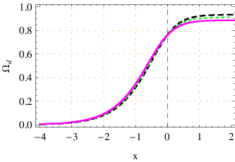
,
3.2.2
In this case and equation (40), (41) and (43) reduce to
| (51) | |||||
| (52) | |||||
| (53) |
where
From the above equations are seen that when , , , tend to , , respectively. We see that at the early time and are divergent.
The equation of motion for is
| (54) |
Its analytical solution gives
| (55) |
where
| (56) | |||||
| (57) |
and is the integration constant.


3.2.3
In this case and equation(40), (41) and (43) reduce to
| (58) | |||||
| (59) | |||||
| (60) |
where
It is seen that the quantity , , have the same behavior which we obtain for . This means that and are divergent in the early time.
Finally in this case the equation of motion for dimensionless density energy parameter is
| (61) |
Integration (47), gives
| (62) |
where
| (63) | |||||
| (64) |
and
We plot versus for and in figure 7. These two sub-figures show that the behavior of versus is similar for two different kinds of interaction and also they show the evolution of Universe is completely in positive accelerating expansion phase, because is always less than . These figures indicate will increase from to a local maximum below and then decrease to the below of . This means that cross the line two times. One time from phantom phase to quintessence phase nearly at early time and another time from quintessence phase to phantom phase in which at the present ( the second crossing has took place.
Figures 8(a) and 8(b) show the squared sound speed versus for and respectively. These figures indicate is negative in for these two kinds of interaction, and for one can obtain a positive value for by a suitable choice of parameter. This means that for these two kinds of interaction the GDE model is stable in the present time in the context of CBD model of gravity.
4 Conclusion
Recently, Ghost dark energy is introduced [19]. This kind of dark energy is a phenomenological vacuum energy which is rooted from the Veneziano ghost of QCD. The ghost dark energy model is proportional to Hubble parameter. According to results of [21], the adiabatic squared sound speed of the GDE model in the context of Einsteinian theory of gravity is negative and then this model is instable. And also it is shown that this model has a behavior like a cosmological constant at the late time () and the equation of state can never cross . We study the stability and the evolution of this model in the context of Brans-Dicke model which has non-minimal coupling with matter, namely chameleon Brans-Dicke (GDECBD) model. At first, we investigated the GDE of CBD model without any interaction between GDE and CDM in a non flat FLRW metric. In this investigation we obtain the EoS parameter, deceleration parameter, the equation of motion for GDE fraction parameter and the adiabatic squared sound speed of the model. The obtained quantities show that the GDE model in the context of CBD scenario can describe the positive accelerating expansion phase of Universe and the EoS parameter of dark energy can cross the phantom divide line, also the squared sound speed of the DE is positive, for a suitable choice if parameter. We studied the cosmological dynamics of the model by considering three usual forms of interaction between DE and CDM. Considering the evolution of dimensionless density energy parameter, we have shown that varies from 0 at early time to 1 at late time. We fund that the evolution of Universe in GDE model of CBD scenario is completely in positive accelerating expansion phase for three forms of interaction. Also we obtained crosses the line from phantom phase to quintessence phase for case, but the behavior of versus is similar for and and also cross the line two times. One time from phantom phase to quintessence phase nearly at early time and another time from quintessence phase to phantom phase in which at the present ( the second crossing has took place.
Finally we found the squared sound speed of GDE model in CBD framework for three kinds of interaction in the FRW Universe. All of our calculations show that is negative in and for one can obtain a positive value for by a suitable choice of parameter. This means that the interacting and non-interacting case of GDE model is stable in the present time in the context of CBD model of gravity.
5 Aknowledgement
The work of Kh. Saaidi have been supported financially by University of Kurdistan, Sanandaj, Iran, and he would like thank to the University of Kurdistan for supporting him in sabbatical period.
References
- [1] A. G. Reiss et al., Astron. J. 116, 1009 (1998); S. Perlumutter et al., Bull. Am. Astron. Soc. 29, 1351 (1997); P. de Bernardis et al., Nature 404, 955 (2000).
- [2] S. Bridle, O. Lahav, J. P. Ostriker and P. J. steinhardt, Scince 299, 1532 (2003.
- [3] G. J. Sobczak et al.,[astro-ph/9903395].
- [4] K. Abazajian et al., [SDSS Collaboration], Astron. J. 128, 502 (2004); K. Abazajian et al., [SDSS Collaboration], Astron. J.129, 1755 (2005).
- [5] S. Weinberg, Rev. Mod. Phys. 61, 1 (1989); P. J. E. Peebles and B. Ratra, Rev. Mod. Phys. 75, 559 (2003); S. M. Carroll, Living Rev. Rel. 4, 1 (2001).
- [6] P. J. Steinhardt, in critical problems in physics, edited by V. L. Fitch and D. R. Marlow (Printed University Press, Prinston, NJ, (1997); P. J. Steinhardt, et al Princeton university press, Princeton U. S. A.
- [7] D. F. Mota and J. D. Barrow, Phys. Lett. B 581, 141 (2004); J. Khoury and A. Weltman, Phys. Rev. D 69, 044026 (2004), Phys. Rev. Lett. 93, 171104 (2004).
- [8] P. J. E. Peebles and B. Ratra, Astrophys. J. L 17, 325 (1988); B. Ratra and P. J. E. Peebles, Phys. Rev. D 37, 3406 (1988); T. G. Clemson and A. R. Liddle, Mon. Not. Roy. Astron. Soc. 395, 1585 (2009); C. Wetterich, Nucl. Phys. B 302, 668 (1988).
- [9] C. Armendariz-Picon, V. F. Mukhanov and P. J. Steinhardt, Phys. Rev. Lett. 85, 4438 (2000); T. Chiba, T. Okabe and M. Yamaguchi, Phys. Rev. D 62, 023511 (2000); C. Armendariz-Picon, V. F. Mukhanov and P. J. Steinhardt, Phys. Rev. D 63, 103510 (2001).
- [10] A. Sen, JHEP 0207, 065 (2002).
- [11] N. Arkani-Hamed et al., JHEP 0405, 074 (2004); F. Piazza and S. Tusjikawa, JCAP 0407, 004 (2004).
- [12] R. R. Caldwell, Phys. Lett. B 545, 23 (2002).
- [13] E. Elizalde, S. Nojiri and S. D. Odintsov, Phys. Rev. D 70, 043539 (2004)
- [14] A. Kamenshchik, U. Moschella and V. Pasquier, Phys. Lett. B 511, 265 (2001); M. C. Bento, O. Bertolami and A. A. Sen, Phys. Rev. D 66, 043507, (2002).
- [15] H. Wei and R.G. Cai, Phys. Lett. B 660, 113 (2008); K. Nozari and T. Azizi, Phys. Lett .B 680, 2051 (2009); K. Y. Kim, H. W. Lee and Y. S. Myung, Phys. Lett. B 660, 118 (2008); J. P. Wu, D. Z. Ma and Y. Ling, Phys. Lett. B 663, 152 (2008); Y. W. Kim et al., Mod. Phys. Lett. A 23, 3049 (2008).
- [16] C. Brans and R. H. Dicke, Phys. Rev., 124, 925 (1962).
- [17] Ph. Brax, C. Van de Bruck, A. C. Davis, J. Khoury and A. Weltman, [astro-ph/0410103].
- [18] F. R. Urban and A. R. Zhitnitsky, Phys. Lett. B 688, 9 (2010), Phys. Rev. D 80, 063001 (2009), JCAP 0909, 018 (2009), Nucl. Phys. B 835, 135 (2010).
- [19] N. Ohta,Phys. Lett. B 695, 41 (2011).
- [20] E. Witten, Nucl. Phys. B 156, 269 (1979); G. Veneziano, Nucl. Phys. B 159, 213 (1979); C. Rosenzweig, J. Schechter and C. G. Trahern, Phys. Rev. D 21, 3388 (1980); P. Nath and R. L. Arnowitt, Phys. Rev. D 23, 473 (1981); K. Kawarabayashi and N. Ohta, Nucl. Phys. B 175, 477 (1980).
- [21] R. G. Cai, Z. L. Tuo, H. B. Zhang, arXiv:1011.3212; E. Ebrahimi, A. Sheykhi, Phys. Lett. B 705, 19 (2011), Int. J. Mod. Phys. D 20, 2369 (2011).
- [22] P. J. E. Peebles and B. Ratra, Rev. Mod. Phys. 75, 559 (2003).
- [23] V. Gorini, A. Kamenshchik, U. Moschella, V. Pasquier and A. Starobinsky, Phys. Rev. D 72, 103518 (2005).
- [24] Y. S. Myung, Phys. Lett. B 652, 223 (2007).
- [25] O. Bertolami, F. G. Pedro and M. Le Delliou, Phys. Lett. B 654, 165 ( 2007).
- [26] B. F. Schutz, Phys. Rev. D 2, 2762 (1970); J. D. Brown, Class. Quant. Grav. 10, 1579 (1993); S. W. Hawking and G. F. R. Ellis, ”The Large Scale Structure of Spacetime”, (Cambridge University Press, Cambridge 1973).
- [27] N. Banerjee and D. Pavon, Phys. Lett. B 647, 447 (2007).
- [28] N. Banerjee and D. Pav´on, Phys .Rev .D 63, 043504 (2001); Class. Quantum Grav. 18, 593 (2001).
- [29] V. Acquaviva, L. Verde, JCAP 12, 001 (2007).
- [30] F. Wu, X. Chen, Phys. Rev. D 82, 083003 (2010).