跳到论文正文
W Papers独立论文阅读器 arXiv:1202.4000 论文正文 计算阅读时间 · 0%
引用这篇论文根据当前论文元数据生成,正式投稿前建议核对。


License: arXiv.org perpetual non-exclusive license
arXiv:1202.4000v2 [math.CA] 20 Feb 2012

High order three-term recursions, Riemann-Hilbert minors and Nikishin systems on star-like sets

Steven Delvaux11 1 Department of Mathematics, University of Leuven (KU Leuven), Celestijnenlaan 200B, B-3001 Leuven, Belgium. email: {steven.delvaux, abey.lopezgarcia}@wis.kuleuven.be. The authors are Postdoctoral Fellows of the Fund for Scientific Research-Flanders (FWO), Belgium.    Abey López11 1 Department of Mathematics, University of Leuven (KU Leuven), Celestijnenlaan 200B, B-3001 Leuven, Belgium. email: {steven.delvaux, abey.lopezgarcia}@wis.kuleuven.be. The authors are Postdoctoral Fellows of the Fund for Scientific Research-Flanders (FWO), Belgium.
August 24, 2026
Abstract

We study monic polynomials Qn​(x)Q_{n}(x) generated by a high order three-term recursion x​Qn​(x)=Qn+1​(x)+an−p​Qn−p​(x)xQ_{n}(x)=Q_{n+1}(x)+a_{n-p}Q_{n-p}(x) with arbitrary p≥1p\geq 1 and an>0a_{n}>0 for all nn. The recursion is encoded by a two-diagonal Hessenberg operator HH. One of our main results is that, for periodic coefficients ana_{n} and under certain conditions, the QnQ_{n} are multiple orthogonal polynomials with respect to a Nikishin system of orthogonality measures supported on star-like sets in the complex plane. This improves a recent result of Aptekarev-Kalyagin-Saff where a formal connection with Nikishin systems was obtained in the case when ∑n=0∞|an−a|<∞\sum_{n=0}^{\infty}|a_{n}-a|<\infty for some a>0a>0.

An important tool in this paper is the study of ‘Riemann-Hilbert minors’, or equivalently, the ‘generalized eigenvalues’ of the Hessenberg matrix HH. We prove interlacing relations for the generalized eigenvalues by using totally positive matrices. In the case of asymptotically periodic coefficients ana_{n}, we find weak and ratio asymptotics for the Riemann-Hilbert minors and we obtain a connection with a vector equilibrium problem. We anticipate that in the future, the study of Riemann-Hilbert minors may prove useful for more general classes of multiple orthogonal polynomials.

Keywords: Multiple orthogonal polynomial, Nikishin system, banded Hessenberg matrix, block Toeplitz matrix, Riemann-Hilbert matrix, generalized Poincaré theorem, ratio asymptotics, vector equilibrium problem, interlacing, totally positive matrix.

MSC 2010: Primary 42​C​0542C05; Secondary 15​B​0515B05, 15​B​4815B48.

1 Introduction

Let (Qn)n=0∞(Q_{n})_{n=0}^{\infty} be the sequence of monic polynomials generated by the recurrence relation

x​Qn​(x)=Qn+1​(x)+an−p​Qn−p​(x),n≥0,xQ_{n}(x)=Q_{n+1}(x)+a_{n-p}Q_{n-p}(x),\qquad n\geq 0, (1.1)

for a fixed integer p∈ℕ:={1,2,3,…}p\in\mathbb{N}:=\{1,2,3,\ldots\}, with initial conditions

Q0​(x)≡1,Q−1​(x)≡⋯≡Q−p​(x)≡0.Q_{0}(x)\equiv 1,\qquad Q_{-1}(x)\equiv\cdots\equiv Q_{-p}(x)\equiv 0. (1.2)

The recurrence coefficients ana_{n} are assumed to be positive real numbers:

an>0,n≥0.a_{n}>0,\qquad n\geq 0. (1.3)

Note that for p=1p=1, (1.1) reduces to the standard three-term recurrence relation for orthogonal polynomials on the real line, in the special case of an even orthogonality measure. We will be interested in the case where p≥2p\geq 2, which we refer to as a high order three-term recurrence [1].

The assumption (1.3) implies that the zeros of QnQ_{n} are located on the star S+:={x∈ℂ∣xp+1∈ℝ+},S_{+}:=\{x\in\mathbb{C}\mid x^{p+1}\in\mathbb{R}_{+}\}, and that they satisfy certain interlacing relations. This was demonstrated by Eiermann-Varga [12] and Romdhane [24]; see also Fig. 1 and 2 below for the case p=2p=2. In the present paper we will obtain more general interlacing relations, in the context of so-called Riemann-Hilbert minors.

The polynomials QnQ_{n} are studied in the literature under various assumptions on the recurrence coefficients ana_{n}. He and Saff [16] show that the Faber polynomials associated with the closed domain bounded by a (p+1)(p+1)-cusped hypocycloid satisfy the recursion (1.1) with constant coefficients an=a=1/pa_{n}=a=1/p. Many properties of these Faber polynomials are obtained in [12, 16].

More properties and applications for the polynomials QnQ_{n} are obtained by Ben Cheikh-Douak [3], Douak-Maroni [9], Maroni [20] and others [22, 24]. The polynomials QnQ_{n} are often called dd-symmetric dd-orthogonal polynomials in these references (with d:=pd:=p). An application from the normal matrix model is given in [5].

General considerations [10, 17] show that the polynomials QnQ_{n} satisfy formal multiple orthogonality relations with respect to certain linear functionals. Aptekarev, Kalyagin and Van Iseghem [2] obtain a stronger version of this result:

Theorem 1.1.

(See [1, Th. 1.1], [2, Cor. 2]:) Suppose that an>0a_{n}>0 for all nn and the numbers ana_{n} are uniformly bounded. Then the polynomials Qn​(x)Q_{n}(x) are multiple orthogonal with respect to the measures ν1,…,νp\nu_{1},\ldots,\nu_{p} defined in (8.3) (see Section 8), in the sense that

∫Qn​(x)​xm​d​νj​(x)=0,\int Q_{n}(x)x^{m}\,\mathrm{d}\nu_{j}(x)=0, (1.4)

for any m∈[0:⌊n−jp⌋]m\in[0:\lfloor\frac{n-j}{p}\rfloor] and j∈[1:p]j\in[1:p].

Here x↦⌊x⌋x\mapsto\lfloor x\rfloor denotes the ‘floor’ function and we abbreviate [i:j]:={i,i+1,…,j}[i:j]:=\{i,i+1,\ldots,j\}. This notation will be used throughout the paper.

The measures ν1,…,νp\nu_{1},\ldots,\nu_{p} are supported on a compact subset of the star S+S_{+}. We will call them the orthogonality measures. Aptekarev, Kalyagin and Saff [1] study these measures in the case where ∑n=0∞|an−a|<∞\sum_{n=0}^{\infty}|a_{n}-a|<\infty for some a>0a>0. They obtain a formal link with Nikishin systems. In the present paper we will extend this link to the case of periodic ana_{n}. In particular, we will obtain conditions guaranteeing that ν1,…,νp\nu_{1},\ldots,\nu_{p} form a true, rather than a formal, Nikishin system.

For any j∈[1:p],j\in[1:p], define the second kind function Ψn(j)\Psi_{n}^{(j)} by

Ψn(j)​(z):=∫Qn​(t)z−t​d​νj​(t),n≥0.\Psi_{n}^{(j)}(z):=\int\frac{Q_{n}(t)}{z-t}\,\mathrm{d}\nu_{j}(t),\qquad n\geq 0. (1.5)

Define the Riemann-Hilbert matrix (briefly RH matrix) Yn​(z)Y_{n}(z) by

Yn​(z)=(Qn​(z)Ψn(1)​(z)…Ψn(p)​(z)Qn−1​(z)Ψn−1(1)​(z)…Ψn−1(p)​(z)Qn−p​(z)Ψn−p(1)​(z)…Ψn−p(p)​(z)).Y_{n}(z)=\begin{pmatrix}Q_{n}(z)&\Psi_{n}^{(1)}(z)&\ldots&\Psi_{n}^{(p)}(z)\\ Q_{n-1}(z)&\Psi_{n-1}^{(1)}(z)&\ldots&\Psi_{n-1}^{(p)}(z)\\ \vdots&\vdots&&\vdots\\ Q_{n-p}(z)&\Psi_{n-p}^{(1)}(z)&\ldots&\Psi_{n-p}^{(p)}(z)\end{pmatrix}. (1.6)

This definition is a variant of the one in Van Assche, Geronimo and Kuijlaars [28], see also [13]. The matrix Yn​(z)Y_{n}(z) satisfies a certain Riemann-Hilbert problem; but we will not need this here.

Denote the principal (k+1)×(k+1)(k+1)\times(k+1) minor of Yn​(z)Y_{n}(z) by

Bk,n​(z)=det(Qn​(z)Ψn(1)​(z)…Ψn(k)​(z)Qn−k​(z)Ψn−k(1)​(z)…Ψn−k(k)​(z)),B_{k,n}(z)=\det\begin{pmatrix}Q_{n}(z)&\Psi_{n}^{(1)}(z)&\ldots&\Psi_{n}^{(k)}(z)\\ \vdots&\vdots&&\vdots\\ Q_{n-k}(z)&\Psi_{n-k}^{(1)}(z)&\ldots&\Psi_{n-k}^{(k)}(z)\end{pmatrix}, (1.7)

for k∈[0:p]k\in[0:p]. We call this the kkth principal Riemann-Hilbert minor of YnY_{n}. For n<kn<k we set Bk,n​(z)≡1B_{k,n}(z)\equiv 1. In this paper we will also work with the determinants of more general submatrices of (1.6), whose rows are not necessarily consecutive; see Section 3 and following.

Lemma 1.2.

For any k∈[0:p]k\in[0:p], Bk,n​(x)B_{k,n}(x) is a polynomial of degree

deg⁡Bk,n≤p−kp​(n−k).\deg B_{k,n}\leq\frac{p-k}{p}(n-k).
Proof.

First we prove that Bk,n​(x)B_{k,n}(x) is a polynomial. By the multi-linearity of the determinant,

Bk,n(z)=∫⋯∫det(Qn​(z)Qn​(y1)…Qn​(yk)Qn−k​(z)Qn−k​(y1)…Qn−k​(yk))d​ν1​(y1)​…​d​νk​(yk)(z−y1)⋯(z−yk).B_{k,n}(z)=\int\cdots\int\det\begin{pmatrix}Q_{n}(z)&Q_{n}(y_{1})&\ldots&Q_{n}(y_{k})\\ \vdots&\vdots&&\vdots\\ Q_{n-k}(z)&Q_{n-k}(y_{1})&\ldots&Q_{n-k}(y_{k})\end{pmatrix}\frac{\,\mathrm{d}\nu_{1}(y_{1})\ldots\,\mathrm{d}\nu_{k}(y_{k})}{(z-y_{1})\cdots(z-y_{k})}.

The integrand is clearly a polynomial in zz, hence Bk,nB_{k,n} is a polynomial. Finally, the claim about the degree of Bk,n​(z)B_{k,n}(z) will be a consequence of Prop. 2.6 and Lemma 2.5 in what follows. (This claim may be shown in a direct way as well.) ∎

Note in particular that deg⁡Bp,n=0\deg B_{p,n}=0, i.e., the determinant of the full RH matrix Yn​(z)Y_{n}(z) is a constant. Prop. 2.6 will imply that this constant is nonzero.

Define the two complementary ‘stars’

S±:={x∈ℂ∣xp+1∈ℝ±}.S_{\pm}:=\{x\in\mathbb{C}\mid x^{p+1}\in\mathbb{R}_{\pm}\}. (1.8)

In this paper we will prove that the zeros of Bk,nB_{k,n} (and of more general RH minors) are all located on the star S+S_{+} if kk is even and on the star S−S_{-} if kk is odd. We will also obtain several kinds of interlacing relations between the zeros of the different RH minors.

The main focus of this paper is on the case where the recurrence coefficients ana_{n} are asymptotically periodic of period r∈ℕr\in\mathbb{N}. This means that

limn→∞ar​n+j=:bj>0,j∈[0:r−1],\lim_{n\to\infty}a_{rn+j}=:b_{j}>0,\qquad j\in[0:r-1], (1.9)

for certain limiting values b0,…,br−1>0b_{0},\ldots,b_{r-1}>0.

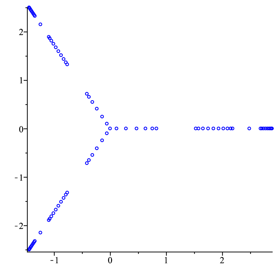
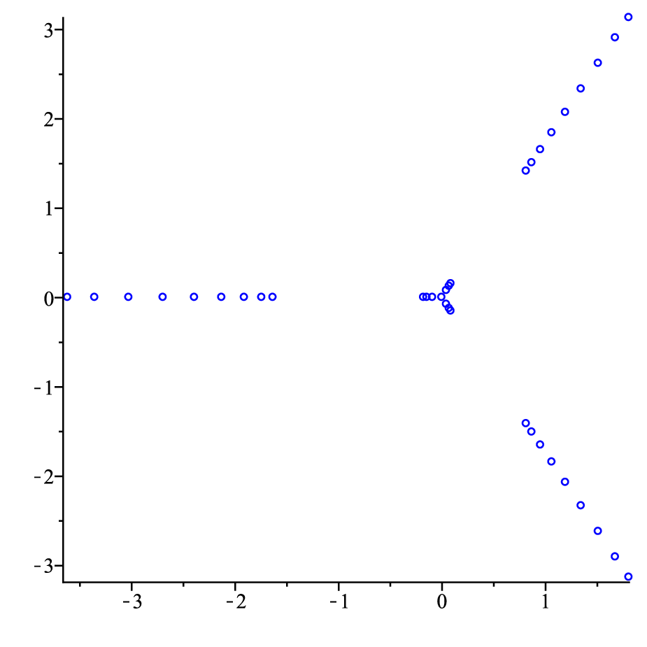
It turns out that in the asymptotically periodic case, the zeros of QnQ_{n} for n→∞n\to\infty are attracted (in the sense of weak convergence) by a certain rotationally invariant subset Γ0\Gamma_{0} of the star S+S_{+}. Moreover, the zeros asymptotically distribute themselves according to a measure μ0\mu_{0} on Γ0\Gamma_{0}, which appears in the solution to a certain vector equilibrium problem. An example of the set Γ0\Gamma_{0} is shown in the left picture of Fig. 1. Below we will also introduce a family of sets Γk\Gamma_{k} and measures μk\mu_{k}, k∈[0:p−1]k\in[0:p-1], which will be the limiting zero distributions of the RH minors Bk,nB_{k,n}.

Refer to caption
Refer to caption
Figure 1: Zeros of Q80Q_{80} (left) and P1,80P_{1,80} (right) in the periodic case with p=2p=2 and period r=8r=8 and (a0,…,a7)=(3,1,5,2,2,9,6,1)(a_{0},\ldots,a_{7})=(3,1,5,2,2,9,6,1). The zeros of QnQ_{n} accumulate on a set Γ0⊂S+\Gamma_{0}\subset S_{+} whose intersection with ℝ\mathbb{R} is [0,0.85]∪[1.52,2.19]∪[2.67,2.89][0,0.85]\cup[1.52,2.19]\cup[2.67,2.89] (using two digits of precision). The zeros of P1,nP_{1,n} accumulate on a set Γ1⊂S−\Gamma_{1}\subset S_{-} whose intersection with ℝ\mathbb{R} is [−3.72,−1.59]∪[−0.17,0][-3.72,-1.59]\cup[-0.17,0]. Note that Q80Q_{80} has an isolated zero between some of the intervals.

Define the matrix

F⁡(z,x):=Z−1+Zp​diag⁡(b0,…,br−1)−x​Ir,F(z,x):=Z^{-1}+Z^{p}\diag(b_{0},\ldots,b_{r-1})-xI_{r}, (1.10)

and the algebraic curve

0=f⁡(z,x):=detF⁡(z,x),0=f(z,x):=\det F(z,x), (1.11)

where ZZ denotes the cyclic shift matrix

Z=(0zIr−10),Z=\begin{pmatrix}0&z\\ I_{r-1}&0\end{pmatrix}, (1.12)

and where IkI_{k} denotes the identity matrix of size kk. If r=1r=1 then we put Z=zZ=z and b0=:bb_{0}=:b. In that case, (1.11) reduces to the algebraic curve z−1+b​zp−x=0z^{-1}+bz^{p}-x=0 in [1, 16]. The matrix F⁡(z,x)F(z,x) can be interpreted as the symbol of a block Toeplitz matrix. This is explained in Section 6.

The expression f⁡(z,x)f(z,x) can be expanded as a Laurent polynomial in zz:

f⁡(z,x)=(−1)r−1​z−1+𝖿0​(x)+𝖿1​(x)​z+⋯+𝖿p​(x)​zp,f(z,x)=(-1)^{r-1}z^{-1}+\mathsf{f}_{0}(x)+\mathsf{f}_{1}(x)z+\cdots+\mathsf{f}_{p}(x)z^{p}, (1.13)

where each 𝖿k​(x)\mathsf{f}_{k}(x), k∈[0:p]k\in[0:p], is a polynomial in xx, and

𝖿p​(x)≡𝖿p=(−1)p⁡(r−p)​∏k=0r−1bk.\mathsf{f}_{p}(x)\equiv\mathsf{f}_{p}=(-1)^{p(r-p)}\prod_{k=0}^{r-1}b_{k}. (1.14)

The algebraic equation f⁡(z,x)=0f(z,x)=0 has precisely p+1p+1 roots zk=zk​(x)z_{k}=z_{k}(x), k∈[0:p]k\in[0:p] (counting multiplicities), and we order them by increasing modulus as

|z0​(x)|≤|z1​(x)|≤⋯≤|zp​(x)||z_{0}(x)|\leq|z_{1}(x)|\leq\cdots\leq|z_{p}(x)| (1.15)

for all x∈ℂx\in\mathbb{C}. If x∈ℂx\in\mathbb{C} is such that two or more subsequent roots zk​(x)z_{k}(x) in (1.15) have the same modulus then we may arbitrarily label them so that (1.15) is satisfied. It is easy to see (see e.g. [7, Sec. 4] or [29, p. 102]) that for x→∞x\rightarrow\infty,

z0(x)=x−r+O(x−r−1),zk(x)=O(xr/p),k∈[1:p].z_{0}(x)=x^{-r}+O(x^{-r-1}),\qquad z_{k}(x)=O(x^{r/p}),\quad k\in[1:p]. (1.16)

More precisely, for any x∈ℂx\in\mathbb{C} there is a permutation (z~k​(x))k=1p(\tilde{z}_{k}(x))_{k=1}^{p} of the set (zk​(x))k=1p(z_{k}(x))_{k=1}^{p} so that

z~k(x)p/d=(∏n=0r/d−1bd​n+(k−modd))−1xr/d(1+o(1)),k∈[1:p],\widetilde{z}_{k}(x)^{p/d}=\left(\prod_{n=0}^{r/d-1}b_{dn+(k-1\!\!\!\!\mod\!d)}\right)^{-1}x^{r/d}(1+o(1)),\qquad k\in[1:p], (1.17)

as x→∞x\to\infty, where d:=gcd⁡{p,r}d:=\gcd\{p,r\}. See [29, p. 102].

Define the sets Γk\Gamma_{k} by

Γk={x∈ℂ∣|zk(x)|=|zk+1(x)|},k∈[0:p−1].\Gamma_{k}=\{x\in\mathbb{C}\mid|z_{k}(x)|=|z_{k+1}(x)|\},\qquad k\in[0:p-1]. (1.18)

It turns out that Γk\Gamma_{k} is a finite union of line segments on the star S+S_{+} if kk is even and S−S_{-} if kk is odd: see Fig. 1 and Theorem 2.2. The next lemma shows that Γk\Gamma_{k} is rotationally invariant.

Lemma 1.3.

(Rotational symmetry:) With ω:=exp⁡(2​π​i/(p+1))\omega:=\exp(2\pi\text{\rm{i}}/(p+1)), we have f⁡(z,ω​x)=ωr​f​(ωr​z,x)f(z,\omega x)=\omega^{r}f(\omega^{r}z,x). Hence, for any x∈ℂx\in\mathbb{C} the sets (zk​(ω​x))k=0p(z_{k}(\omega x))_{k=0}^{p} and (ω−r​zk​(x))k=0p(\omega^{-r}z_{k}(x))_{k=0}^{p} are equal up to permutation, and each set Γk\Gamma_{k} is invariant under rotations over 2​π/(p+1)2\pi/(p+1).

Proof.

Recalling (1.10)–(1.12), it is easy to see that D−1​F​(z,ω​x)​D=ω​F​(ωr​z,x)D^{-1}F(z,\omega x)D=\omega F(\omega^{r}z,x) where D:=diag⁡(1,ω,ω2,…,ωr−1)D:=\diag(1,\omega,\omega^{2},\ldots,\omega^{r-1}). This implies the lemma. ∎

For any k∈[0:p−1]k\in[0:p-1], define the measure

d​μk​(λ)=12​π​i​1r​∑j=0k(zj+′​(λ)zj+​(λ)−zj−′​(λ)zj−​(λ))​d​λ\,\mathrm{d}\mu_{k}(\lambda)=\frac{1}{2\pi\text{\rm{i}}}\frac{1}{r}\sum_{j=0}^{k}\left(\frac{z_{j+}^{\prime}(\lambda)}{z_{j+}(\lambda)}-\frac{z_{j-}^{\prime}(\lambda)}{z_{j-}(\lambda)}\right)\,\mathrm{d}\lambda (1.19)

supported on Γk\Gamma_{k}. Here the prime denotes the derivative with respect to λ\lambda, and d​λ\,\mathrm{d}\lambda denotes the complex line element on each line segment of Γk\Gamma_{k}, according to some fixed orientation of Γk\Gamma_{k}. Moreover, zj+​(λ)z_{j+}(\lambda) and zj−​(λ)z_{j_{-}}(\lambda) are the boundary values of zj​(λ)z_{j}(\lambda) obtained from the ++-side and −--side respectively of Γk\Gamma_{k}, where the ++-side (−--side) is the side that lies on the left (right) when moving through Γk\Gamma_{k} according to its orientation. It turns out that μk\mu_{k} is a positive measure (obviously independent of the orientation given to Γk\Gamma_{k}) with total mass [7, Sec. 4]

μk(Γk)=p−kp,k∈[0:p−1].\mu_{k}(\Gamma_{k})=\frac{p-k}{p},\qquad k\in[0:p-1]. (1.20)

The measures (μk)k(\mu_{k})_{k} are the minimizers to an equilibrium problem that we now describe. For any measures μ,ν\mu,\nu on ℂ\mathbb{C} define their mutual logarithmic energy as

I⁡(μ,ν)=∫∫⁡log⁡1|x−y|​𝑑μ​(x)​𝑑ν​(y).I(\mu,\nu)=\int\int\ \log\frac{1}{|x-y|}\ \,\mathrm{d}\mu(x)\ \,\mathrm{d}\nu(y).

The logarithmic energy of the measure μ\mu is defined as I⁡(μ)=I⁡(μ,μ)I(\mu)=I(\mu,\mu).

We call a vector of positive measures ν→=(ν0,…,νp−1)\vec{\nu}=(\nu_{0},\ldots,\nu_{p-1}) admissible if νk\nu_{k} has finite logarithmic energy, νk\nu_{k} is supported on Γk\Gamma_{k}, and νk\nu_{k} has total mass νk​(Γk)=p−kp\nu_{k}(\Gamma_{k})=\frac{p-k}{p}, k∈[0:p−1]k\in[0:p-1]. The energy functional JJ is defined by

J⁡(ν→)=∑k=0p−1I⁡(νk)−∑k=0p−2I⁡(νk,νk+1).J(\vec{\nu})=\sum_{k=0}^{p-1}I(\nu_{k})-\sum_{k=0}^{p-2}I(\nu_{k},\nu_{k+1}). (1.21)

The (vector) equilibrium problem is to minimize the energy functional (1.21) over all admissible vectors of positive measures ν→\vec{\nu}. The equilibrium problem has a unique solution which is given by the measures μk\mu_{k} in (1.19), see [7].

2 Statement of results

2.1 Limiting zero distribution of Riemann-Hilbert minors

Denote the normalized zero counting measure of Bk,nB_{k,n}, k∈[0:p−1]k\in[0:p-1], by

μk,n:=1n​∑x|Bk,n​(x)=0δx,\displaystyle\mu_{k,n}:=\frac{1}{n}\sum_{x\mid B_{k,n}(x)=0}\delta_{x}, (2.1)

where δx\delta_{x} is the Dirac measure at xx and each zero is counted according to its multiplicity. Lemma 1.2 shows that μk,n\mu_{k,n} has total mass at most (p−k)/p(p-k)/p. Now we state our first main theorem.

Theorem 2.1.

Assume we have asymptotically periodic recurrence coefficients (1.9), and define μk,n\mu_{k,n}, μk\mu_{k} as in (2.1) and (1.19). Then for any k∈[0:p−1]k\in[0:p-1], the measures μk,n\mu_{k,n} weakly converge to the measure μk\mu_{k} on Γk\Gamma_{k} as n→∞n\to\infty. This means that

limn→∞∫ϕ⁡(x)​d​μk,n​(x)=∫ϕ⁡(x)​d​μk​(x)\lim_{n\to\infty}\int\phi(x)\,\mathrm{d}\mu_{k,n}(x)=\int\phi(x)\,\mathrm{d}\mu_{k}(x) (2.2)

for any bounded continuous function ϕ\phi.

Theorem 2.1 will be proved in Section 7 with the help of a ‘normal family’ estimate for the ratio of two RH minors (Section 5), and using the generalized Poincaré theorem. In fact, we will use a multi-column version of the generalized Poincaré theorem (Lemma 7.2). This approach yields not only weak asymptotics but also ratio asymptotics for the RH minors, as we explain in Section 7, see e.g. (7.23) or (7.28). Moreover, we will see that Theorem 2.1 remains valid with Bk,nB_{k,n} replaced by more general RH minors (Remark 7.7).

We point out that Theorem 2.1 for k=0k=0 could also be obtained from the normal family arguments in [4], taking into account the interlacing relations for the zeros of QnQ_{n}.

Theorem 2.1 shows that the limiting zero distribution of each Riemann-Hilbert minor Bk,nB_{k,n} exists and that the limiting measures are the minimizers to a vector equilibrium problem. We have reason to believe that a similar conclusion may hold for more general classes of multiple orthogonal polynomials. This may be an interesting topic for further research.

2.2 Star-like structure of Γk\Gamma_{k}

Theorem 2.2.

Assume that (1.9) holds. Fix k∈[0:p−1]k\in[0:p-1] and define Γk\Gamma_{k} (1.18) and also

Γ~k=Γkp+1:={xp+1∣x∈Γk}.\widetilde{\Gamma}_{k}=\Gamma_{k}^{p+1}:=\{x^{p+1}\mid x\in\Gamma_{k}\}. (2.3)

Then:

  • (a)

    Γ~k\widetilde{\Gamma}_{k} is part of ℝ+\mathbb{R}_{+} (or ℝ−\mathbb{R}_{-}) if kk is even (or odd respectively).

  • (b)

    Γ~k\widetilde{\Gamma}_{k} is the union of nkn_{k} intervals Ij,kI_{j,k}:

    Γ~k=⋃j=1nkIj,k,with​nk=⌈k+1p+1​r⌉−⌊k​rp⌋,\widetilde{\Gamma}_{k}=\bigcup_{j=1}^{n_{k}}I_{j,k},\qquad\textrm{with}\ n_{k}=\left\lceil\frac{k+1}{p+1}r\right\rceil-\left\lfloor\frac{kr}{p}\right\rfloor, (2.4)

    with x↦⌈x⌉x\mapsto\lceil x\rceil and x↦⌊x⌋x\mapsto\lfloor x\rfloor denoting the ‘ceiling’ and ‘floor’ functions. The intervals Ij,kI_{j,k}, j∈[1:nk]j\in[1:n_{k}] are pairwise disjoint except maybe for common endpoints.

  • (c)

    The following conditions imply that Γ~k\widetilde{\Gamma}_{k} contains 00 or ∞\infty:

    k+1p+1​r∉ℕ⇒0∈Γ~k,k​rp∉ℕ∪{0}⇒(−1)k​∞∈Γ~k.\frac{k+1}{p+1}r\not\in\mathbb{N}\Rightarrow 0\in\widetilde{\Gamma}_{k},\qquad\frac{kr}{p}\not\in\mathbb{N}\cup\{0\}\Rightarrow(-1)^{k}\infty\in\widetilde{\Gamma}_{k}. (2.5)

Theorem 2.2 was formulated for the sets Γ~k\widetilde{\Gamma}_{k} in (2.3). In terms of the original sets Γk\Gamma_{k}, it implies that Γk\Gamma_{k} lies on one of the two stars S+S_{+} and S−S_{-} in (1.8), depending on whether kk is even or odd respectively. Recall that Γk\Gamma_{k} is rotationally invariant (Lemma 1.3).

Theorem 2.2 will be proved in Section 7.3. In the case r=1r=1 it was already obtained by Aptekarev-Kalyagin-Saff [1]; note that in that case we have n0=⋯=np−1=1n_{0}=\cdots=n_{p-1}=1, Γ~0=[0,c]\widetilde{\Gamma}_{0}=[0,c] for a certain c>0c>0, and Γ~k=(−1)k​ℝ+\widetilde{\Gamma}_{k}=(-1)^{k}\mathbb{R}_{+} for k∈[1:p−1]k\in[1:p-1].

Remark 2.3.

As mentioned in the statement of the theorem, the intervals Ij,kI_{j,k}, j∈[1:nk]j\in[1:n_{k}] in (2.4) are pairwise disjoint except possibly for common endpoints. We believe that such common endpoints are rare, in the sense that for a sufficiently ‘generic’ choice of the parameters bk>0b_{k}>0, k∈[0:r−1]k\in[0:r-1], all the endpoints of the intervals are distinct.

Remark 2.4.

Suppose p=2p=2. Then we have two values k=0k=0 and k=1k=1, and (2.4) reduces to

n0=⌈r3⌉,n1=⌈2​r3⌉−⌊r2⌋.n_{0}=\left\lceil\frac{r}{3}\right\rceil,\qquad n_{1}=\left\lceil\frac{2r}{3}\right\rceil-\left\lfloor\frac{r}{2}\right\rfloor.

For example, if the period r=6r=6 then we have n0=2n_{0}=2 and n1=1n_{1}=1. Note that this is the same setting as in [19], but in the latter paper there is an additional structure on the bk>0b_{k}>0 which implies that the two intervals of Γ~0\widetilde{\Gamma}_{0} are tangent (and contain the origin), so that Γ~0\widetilde{\Gamma}_{0} consists of a single contiguous interval in that case. If the period r=8r=8 then we have n0=3n_{0}=3 and n1=2n_{1}=2: see Fig. 1.

2.3 Generalized eigenvalues and interlacing

To obtain interlacing relations for the zeros of RH minors, we will use an alternative representation via generalized eigenvalue determinants that we now describe. To the recurrence (1.1) we associate the Hessenberg operator H=(Hi,j)i,j=0∞H=(H_{i,j})_{i,j=0}^{\infty} with entries

{Hj−1,j=1,j≥1,Hj+p,j=aj,j≥0,Hi,j=0,otherwise.\left\{\begin{array}[]{llll}H_{j-1,j}&=&1,&j\geq 1,\\ H_{j+p,j}&=&a_{j},&j\geq 0,\\ H_{i,j}&=&0,&\textrm{otherwise}.\end{array}\right. (2.6)

We refer to HH as a two-diagonal Hessenberg matrix. We denote with HnH_{n} its n×nn\times n leading principal submatrix:

Hn=(Hi,j)i,j=0n−1=(010⋱⋱a0⋱⋱⋱⋱10an−p−1…0)n×n.H_{n}=(H_{i,j})_{i,j=0}^{n-1}=\begin{pmatrix}0&1&&&0\\ \vdots&\ddots&\ddots&&\\ a_{0}&&\ddots&\ddots&\\ &\ddots&&\ddots&1\\ 0&&a_{n-p-1}&\ldots&0\end{pmatrix}_{n\times n}. (2.7)

The recurrence relation (1.1) can be written in matrix-vector form as

x​(Q0​(x),Q1​(x),…)T=H​(Q0​(x),Q1​(x),…)T,x(Q_{0}(x),Q_{1}(x),\ldots)^{T}=H(Q_{0}(x),Q_{1}(x),\ldots)^{T}, (2.8)

where the superscript T denotes the transpose. This implies easily that Qn​(x)=det(x​In−Hn).Q_{n}(x)=\det(xI_{n}-H_{n}). So the eigenvalues of HnH_{n} are the zeros of QnQ_{n}.

For k∈[0:p]k\in[0:p] we define the polynomial Pk,n​(x)P_{k,n}(x) as the determinant of the submatrix of Hn−x​InH_{n}-xI_{n} obtained by skipping the first kk rows and the last kk columns. Thus

Pk,n​(x)=det(0…−x1⋱⋱⋱a0⋱⋱⋱⋱⋱⋱1⋱⋱−x⋱⋱an−p−1…0)(n−k)×(n−k).P_{k,n}(x)=\det\begin{pmatrix}0&\ldots&-x&1&&\\ \vdots&\ddots&&\ddots&\ddots&&\\ a_{0}&&\ddots&&\ddots&\ddots&\\ &\ddots&&\ddots&&\ddots&1\\ &&\ddots&&\ddots&&-x\\ &&&\ddots&&\ddots&\vdots\\ &&&&a_{n-p-1}&\ldots&0\end{pmatrix}_{(n-k)\times(n-k)}. (2.9)

The kkth generalized eigenvalues of HnH_{n} are the numbers x∈ℂx\in\mathbb{C} such that Pk,n​(x)=0P_{k,n}(x)=0. For n≤kn\leq k we set Pk,n​(x)≡1P_{k,n}(x)\equiv 1. Note that for k=pk=p we have Pp,n(x)≡a0⋯an−p−1>0P_{p,n}(x)\equiv a_{0}\cdots a_{n-p-1}>0.

Lemma 2.5.

For any k∈[0:p]k\in[0:p], the polynomial Pk,n​(x)P_{k,n}(x) has degree

deg⁡Pk,n≤p−kp​(n−k).\deg P_{k,n}\leq\frac{p-k}{p}(n-k).
Proof.

This follows by a simple combinatorial argument; see e.g. [11, Proof of Prop. 2.5]. ∎

Lemma 2.5 could be refined using the combinatorial formulas in Section 5. This leads to an exact formula for deg⁡Pk,n\deg P_{k,n}, depending on n​mod​pn\ \textrm{mod}\ p. We will not go into this issue here.

The fact of the matter is the following.

Proposition 2.6.

(Generalized eigenvalues versus RH minors:) For any k∈[0:p]k\in[0:p],

Bk,n​(x)=(−1)n⁡(k+1)−(k+12)​ck​Pk,n​(x),B_{k,n}(x)=(-1)^{n(k+1)-\binom{k+1}{2}}c_{k}P_{k,n}(x), (2.10)

cf. (1.7), where the constant ckc_{k} depends only on the first kk moments of the measures ν1,…,νk\nu_{1},\ldots,\nu_{k}:

ck=(−1)k(∫dν1(t))(∫Q1(t)dν2(t))⋯(∫Qk−1(t)dνk(t)).c_{k}=(-1)^{k}\left(\int\,\mathrm{d}\nu_{1}(t)\right)\left(\int Q_{1}(t)\ \,\mathrm{d}\nu_{2}(t)\right)\cdots\left(\int Q_{k-1}(t)\ \,\mathrm{d}\nu_{k}(t)\right). (2.11)

Note that in (2.10) and (2.11), we should understand (12)=0\binom{1}{2}=0 and c0=1c_{0}=1.

We point out that Prop. 2.6 remains valid for arbitrary banded Hessenberg operators, that is, for matrices H=(Hi,j)i,j=0∞H=(H_{i,j})_{i,j=0}^{\infty} defined by

{Hj−1,j=1,j≥1,Hj+k,j=aj(k),j≥0,k∈[0:p],aj(k)∈ℂ,Hi,j=0,otherwise,\left\{\begin{array}[]{ll}H_{j-1,j}=1,&j\geq 1,\\ H_{j+k,j}=a_{j}^{(k)},&j\geq 0,\,\,k\in[0:p],\,\,a_{j}^{(k)}\in\mathbb{C},\\ H_{i,j}=0,&\textrm{otherwise,}\end{array}\right. (2.12)

so that

Hn=(Hi,j)i,j=0n−1=(a0(0)10⋱⋱a0(p)⋱⋱⋱⋱10an−p−1(p)…an−1(0))n×n.H_{n}=(H_{i,j})_{i,j=0}^{n-1}=\begin{pmatrix}a_{0}^{(0)}&1&&&0\\ \vdots&\ddots&\ddots&&\\ a_{0}^{(p)}&&\ddots&\ddots&\\ &\ddots&&\ddots&1\\ 0&&a_{n-p-1}^{(p)}&\ldots&a_{n-1}^{(0)}\end{pmatrix}_{n\times n}. (2.13)

We will assume that aj(p)≠0,a_{j}^{(p)}\neq 0, for all jj, so the entries on the ppth subdiagonal of (2.13) are non-zero. We associate to HH the sequence of monic polynomials (Qn)n=0∞(Q_{n})_{n=0}^{\infty} satisfying the (p+2)(p+2)-term recurrence relation (2.8), i.e.,

x​Qn​(x)=Qn+1​(x)+an(0)​Qn​(x)+an−1(1)​Qn−1​(x)+⋯+an−p(p)​Qn−p​(x),n≥0,xQ_{n}(x)=Q_{n+1}(x)+a_{n}^{(0)}Q_{n}(x)+a_{n-1}^{(1)}Q_{n-1}(x)+\cdots+a_{n-p}^{(p)}Q_{n-p}(x),\qquad n\geq 0, (2.14)

with initial conditions

Q−1≡⋯≡Q−p=0,Q0≡1.Q_{-1}\equiv\cdots\equiv Q_{-p}=0,\quad Q_{0}\equiv 1. (2.15)

Prop. 2.6 will be a consequence of a result proved in Prop. 3.1 for the polynomials QnQ_{n} satisfying (2.14)–(2.15), assuming that these polynomials are multiple orthogonal with respect to a system of pp measures, see Section 3 for more details.

Prop. 2.6 shows that RH minors can be alternatively represented as generalized eigenvalue determinants. We now state interlacing relations for the latter.
Refer to caption
Refer to caption
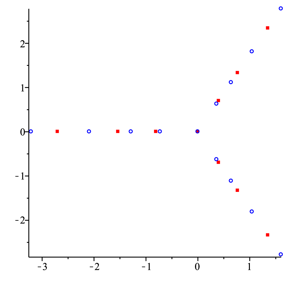
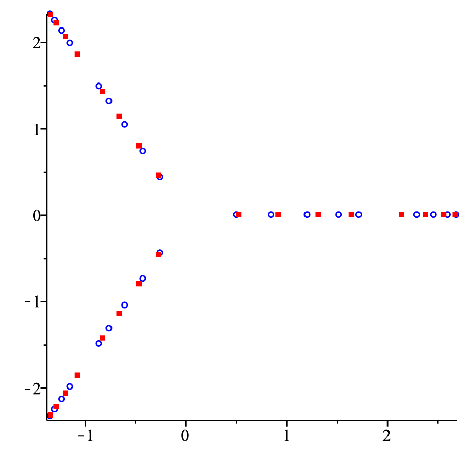
Figure 2: Left picture: zeros of Q23Q_{23} (circles) and Q24Q_{24} (squares). Right picture: zeros of Q24Q_{24} (squares) and Q27Q_{27} (circles). In these pictures we have a two-diagonal Hessenberg matrix HH as in (2.6)–(2.7) with p=2p=2 and recurrence coefficients (a0,…,a5)=(3,2,3,5,4,1)(a_{0},\ldots,a_{5})=(3,2,3,5,4,1) extended periodically with periodicity r=6r=6.
Theorem 2.7.

(Interlacing for generalized eigenvalues:) Let HH be a two-diagonal Hessenberg matrix (2.6) with aj>0a_{j}>0 for all jj. Fix n∈ℕn\in\mathbb{N} and k∈[0:p−1]k\in[0:p-1]. Then

  • (a)

    We have Pk,n​(x)=xmk,n​P~k,n​(xp+1)P_{k,n}(x)=x^{m_{k,n}}\widetilde{P}_{k,n}(x^{p+1}), for a polynomial P~k,n\widetilde{P}_{k,n} with P~k,n​(0)≠0\widetilde{P}_{k,n}(0)\neq 0 and with

    mk,n={(j−k)​(k+1), if n≡jmod(p+1),j∈[k:p],(k−j)​(p−k), if n≡jmod(p+1),j∈[−1:k].m_{k,n}=\left\{\begin{array}[]{ll}(j-k)(k+1),&\textrm{ if }n\equiv j\mod(p+1),\,j\in[k:p],\\[3.00003pt] (k-j)(p-k),&\textrm{ if }n\equiv j\mod(p+1),\,j\in[-1:k].\end{array}\right. (2.16)

    The zeros of P~k,n\widetilde{P}_{k,n} all lie in ℝ+\mathbb{R}_{+} (ℝ−\mathbb{R}_{-}) if kk is even (odd).

  • (b)

    Denote the zeros of P~k,n\widetilde{P}_{k,n} and P~k,n+1\widetilde{P}_{k,n+1} as (xi)i=1,2,…(x_{i})_{i=1,2,\ldots} and (yi)i=1,2,…(y_{i})_{i=1,2,\ldots} respectively, counting multiplicities and ordered by increasing modulus. We have the weak interlacing relation

    0<|x1|≤|y1|≤|x2|≤|y2|≤…0<|x_{1}|\leq|y_{1}|\leq|x_{2}|\leq|y_{2}|\leq\ldots

    if n≡jmod(p+1)n\equiv j\mod(p+1), j∈[k:p−1]j\in[k:p-1], and

    0<|y1|≤|x1|≤|y2|≤|x2|≤…0<|y_{1}|\leq|x_{1}|\leq|y_{2}|\leq|x_{2}|\leq\ldots

    if n≡jmod(p+1)n\equiv j\mod(p+1), j∈[−1:k−1]j\in[-1:k-1].

  • (c)

    Let (xi)i=1,2,…(x_{i})_{i=1,2,\ldots} be the zeros of P~k,n\widetilde{P}_{k,n}, as in (b), and let (wi)i=1,2,…(w_{i})_{i=1,2,\ldots} be the zeros of P~k,n+p+1\widetilde{P}_{k,n+p+1}, counting multiplicities and ordered by increasing modulus. We have

    0<|w1|≤|x1|≤|w2|≤|x2|≤….0<|w_{1}|\leq|x_{1}|\leq|w_{2}|\leq|x_{2}|\leq\ldots.

    Note that the moduli can be removed if kk is even and replaced by minus signs if kk is odd.

Theorem 2.7 generalizes known results for the standard eigenvalues k=0k=0 [12, 24]. The theorem will be proved in Section 4, by using the theory of totally positive matrices and extending the approach of Eiermann-Varga [12]. See also Theorems 2.12 and 4.6 below for related results.
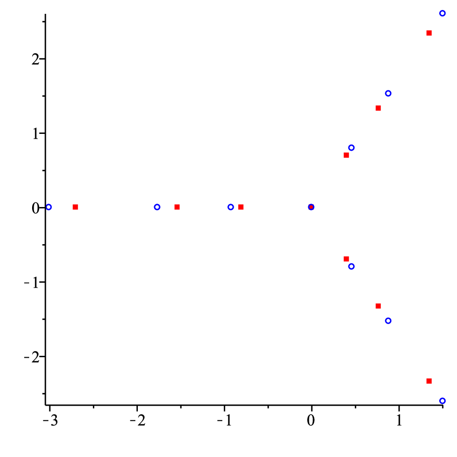
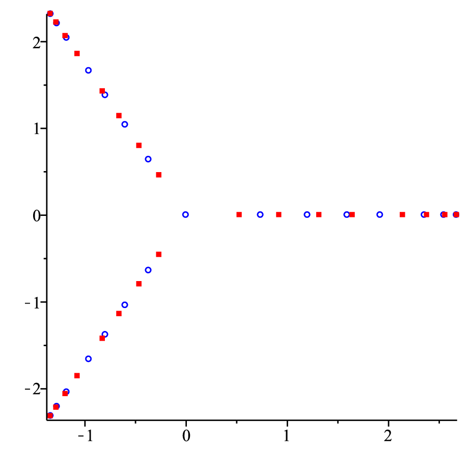
Theorem 2.7 is illustrated in Figures 2 and 3.

Refer to caption
Refer to caption
Figure 3: Left picture: zeros of P1,23P_{1,23} (circles) and P1,24P_{1,24} (squares). Right picture: zeros of P1,24P_{1,24} (squares) and P1,27P_{1,27} (circles). The matrix HH is as in Figure 2.

Generalized eigenvalues turn out to be deeply connected to the hierarchy of functions of the (formal) Nikishin system generated by HH. This will be the topic of Section 2.4.

2.4 Connection with Nikishin systems

Aptekarev-Kalyagin-Saff [1] show that, in the trace class ∑k=0∞|ak−a|<∞\sum_{k=0}^{\infty}|a_{k}-a|<\infty and with period r=1r=1, the two-diagonal operator HH generates a (formal) Nikishin system. These objects are only formally defined however.

In this paper we will obtain a related result. It will apply to the exactly periodic case

ar​n+k=ak=bk,n∈ℕ,k∈[0:r−1].a_{rn+k}=a_{k}=b_{k},\qquad n\in\mathbb{N},\quad k\in[0:r-1]. (2.17)

We assume without loss of generality that the period rr is a multiple of pp. We also assume that

∏n=0r/p−1ap​n>∏n=0r/p−1ap​n+1>⋯>∏n=0r/p−1ap​n+(p−1).\prod_{n=0}^{r/p-1}a_{pn}>\prod_{n=0}^{r/p-1}a_{pn+1}>\cdots>\prod_{n=0}^{r/p-1}a_{pn+(p-1)}. (2.18)

Under these conditions, we will show that the polynomials QnQ_{n} are multiple orthogonal with respect to a true Nikishin system generated by rotationally invariant measures on the stars S+S_{+} and S−S_{-}, coming from measures on ℝ+\mathbb{R}_{+} or ℝ−\mathbb{R}_{-} with constant sign. There can also be possible point masses at each level of the Nikishin hierarchy.

Nikishin systems formed by measures supported on the real line were introduced by E.M. Nikishin in [23]. The same definition can be easily adapted to our context of star-like sets, as we now explain. Compare this definition with the one given in [1, Section 8.1].

Definition 2.8.

Let ν1,…,νp\nu_{1},\ldots,\nu_{p} be a collection of pp complex measures supported on the set Γ0∪𝒜0\Gamma_{0}\cup\mathcal{A}_{0}, where 𝒜0⊂S+∖Γ0\mathcal{A}_{0}\subset S_{+}\setminus\Gamma_{0} is a discrete set. We say that (ν1,…,νp)(\nu_{1},\ldots,\nu_{p}) forms a Nikishin system on (Γ0,…,Γp−1)(\Gamma_{0},\ldots,\Gamma_{p-1}) if for each k∈[0:p−1],k\in[0:p-1], there exists a collection of complex measures (νl,k)l=k+1p(\nu_{l,k})_{l=k+1}^{p} supported on Γk∪𝒜k\Gamma_{k}\cup\mathcal{A}_{k}, where 𝒜k\mathcal{A}_{k} is a discrete subset of S+∖ΓkS_{+}\setminus\Gamma_{k} (if kk is even) or S−∖ΓkS_{-}\setminus\Gamma_{k} (if kk is odd), with the following properties:

  • (a)

    (ν1,…,νp)=(ν1,0,…,νp,0)(\nu_{1},\ldots,\nu_{p})=(\nu_{1,0},\ldots,\nu_{p,0}).

  • (b)

    If d​νl,k​(x)=gl,k​(x)​d​x+d​νl,k(s)​(x)\,\mathrm{d}\nu_{l,k}(x)=g_{l,k}(x)\,\mathrm{d}x+\,\mathrm{d}\nu_{l,k}^{(s)}(x), d​νl,k(s)​(x)⟂gl,k​(x)​d​x\,\mathrm{d}\nu_{l,k}^{(s)}(x)\perp g_{l,k}(x)\,\mathrm{d}x, denotes the Lebesgue decomposition of νl,k\nu_{l,k}, l∈[k+1:p],l\in[k+1:p], then

    gl,k​(x)gk+1,k​(x)=∫d​νl,k+1​(t)x−t,x∈Γk,l∈[k+2:p].\frac{g_{l,k}(x)}{g_{k+1,k}(x)}=\int\frac{\,\mathrm{d}\nu_{l,k+1}(t)}{x-t},\qquad x\in\Gamma_{k},\quad l\in[k+2:p]. (2.19)
  • (c)

    For every l∈[k+1:p],l\in[k+1:p], there exists a real measure ν~l,k\tilde{\nu}_{l,k} with constant sign (either positive or negative), supported on ℝ+\mathbb{R}_{+} (ℝ−\mathbb{R}_{-}) if kk is even (odd), such that

    d​νl,k​(t)=tk+1−l​d​ν~l,k​(tp+1).\,\mathrm{d}\nu_{l,k}(t)=t^{k+1-l}\,\mathrm{d}\tilde{\nu}_{l,k}(t^{p+1}). (2.20)
Remark 2.9.

We observe that Nikishin systems possess a hierarchical structure, with the measures (ν1,…,νp)(\nu_{1},\ldots,\nu_{p}) forming level 00 of the hierarchy. The measure νl,k\nu_{l,k} is said to be at the kkth level of the Nikishin hierarchy. Note that (2.20) implies that for any k∈[0:p−1]k\in[0:p-1], the measure νk+1,k\nu_{k+1,k} is rotationally invariant, and the induced measure ν~k+1,k\tilde{\nu}_{k+1,k} is real with constant sign. The measures νk+1,k\nu_{k+1,k} are usually referred to as the generating measures of the Nikishin system. We are implicitly requiring in (2.19) that gk+1,k​(x)≠0g_{k+1,k}(x)\neq 0 for all but finitely many x∈Γkx\in\Gamma_{k}.

Our main result is the following.

Theorem 2.10.

Let HH be a two-diagonal Hessenberg matrix (2.6) with exactly periodic coefficients aj>0a_{j}>0 satisfying (2.17)–(2.18), where the period rr is a multiple of pp. Then the orthogonality measures (ν1,…,νp)(\nu_{1},\ldots,\nu_{p}) in Theorem 1.1 form a Nikishin system on (Γ0,…,Γp−1)(\Gamma_{0},\ldots,\Gamma_{p-1}) (Def. 2.8). Moreover, the star-like sets (Γk)k=0p−1(\Gamma_{k})_{k=0}^{p-1} are compact and the discrete sets (𝒜k)k=0p−1(\mathcal{A}_{k})_{k=0}^{p-1} are finite.

Theorem 2.10 will be proved in Section 8.

Remark 2.11.

Theorem 2.10 was stated under the condition (2.18). In general, consider the set

{∏n=0r/p−1ap​n,∏n=0r/p−1ap​n+1,⋯,∏n=0r/p−1ap​n+(p−1)}.\left\{\prod_{n=0}^{r/p-1}a_{pn},\prod_{n=0}^{r/p-1}a_{pn+1},\cdots,\prod_{n=0}^{r/p-1}a_{pn+(p-1)}\right\}. (2.21)

Eq. (1.17) (with d=pd=p) shows that there exists a permutation Π\Pi of [1:p][1:p] so that

zΠ⁡(k)(x)=(∏n=0r/p−1ap​n+k−1)−1xr/p(1+o(1)),k∈[1:p],z_{\Pi(k)}(x)=\left(\prod_{n=0}^{r/p-1}a_{pn+k-1}\right)^{-1}x^{r/p}(1+o(1)),\qquad k\in[1:p], (2.22)

for x→∞x\to\infty. This can also be seen from the derivation of (8.26) in Section 8. As a consequence, if the pp numbers in (2.21) are pairwise distinct then all the Γk\Gamma_{k} are bounded. The converse of the last statement is also true, due to [26, Lemma 3.3]. Now if the numbers (2.21) are pairwise distinct but ordered in a different way than (2.18), then a variant to Theorem 2.10 holds. We then have an additional constant or monomial term in the right hand side of (2.19). This is due to the fact that the constant α\alpha in Eq. (8.19) in Section 8 can be nonzero in this case.

We see that the key to obtaining a true (rather than a formal) Nikishin system is to show that the ratio between the densities (2.19) of the measures at the different levels of the Nikishin hierarchy are Cauchy transforms of measures on S+S_{+} or S−S_{-}, associated to real measures with constant sign on ℝ+\mathbb{R}_{+} or ℝ−\mathbb{R}_{-}. We will establish this requirement via a surprising connection with RH minors. In particular we will use the interlacing relations between the zeros of RH minors.

Recall the generalized eigenvalue determinant Pk,n​(x)P_{k,n}(x) from (2.9). We need a more general definition. For any 1≤k≤l≤p1\leq k\leq l\leq p we define Pk,l,n​(x)P_{k,l,n}(x) as the determinant of the submatrix obtained by skipping rows 0,1,…,k−10,1,\ldots,k-1 and columns n−l,n−k+1,n−k+2,…,n−1n-l,n-k+1,n-k+2,\ldots,n-1 of Hn−x​InH_{n}-xI_{n}. If l=kl=k then we retrieve our previous definition: Pk,k,n​(x)≡Pk,n​(x)P_{k,k,n}(x)\equiv P_{k,n}(x).

In the proof of Theorem 2.10 we need the following result on the polynomials Pk,l,n​(x)P_{k,l,n}(x).

Theorem 2.12.

(Interlacing for Pk,l,nP_{k,l,n} and Pk,nP_{k,n}:) Let HH be a two-diagonal Hessenberg matrix (2.6) with aj>0a_{j}>0 for all jj. Fix n∈ℕn\in\mathbb{N} and 0≤k<l≤p0\leq k<l\leq p. Then

  • (a)

    We have Pk,l,n​(x)=xk−l+mk,n​P~k,l,n​(xp+1)P_{k,l,n}(x)=x^{k-l+m_{k,n}}\widetilde{P}_{k,l,n}(x^{p+1}), with mk,nm_{k,n} defined in (2.16) and with P~k,l,n\widetilde{P}_{k,l,n} a polynomial whose zeros all lie in ℝ+\mathbb{R}_{+} (ℝ−\mathbb{R}_{-}) if kk is even (odd).

  • (b)

    Denote the zeros of P~k,n​(x)\widetilde{P}_{k,n}(x) and P~k,l,n​(x)\widetilde{P}_{k,l,n}(x) as (xi)i=1,2,…(x_{i})_{i=1,2,\ldots} and (yi)i=1,2,…(y_{i})_{i=1,2,\ldots} respectively, ordered by increasing modulus and counting multiplicities. We have the weak interlacing relation

    0≤|y1|≤|x1|≤|y2|≤|x2|≤….0\leq|y_{1}|\leq|x_{1}|\leq|y_{2}|\leq|x_{2}|\leq\ldots.

Theorem 2.12 is proved in Section 4. The precise way how Theorem 2.12 is used in the proof of Theorem 2.10 will be explained in Section 8.

Remark 2.13.

The polynomial P~k,l,n\widetilde{P}_{k,l,n} could have one, and at most one, zero at the origin. This happens precisely when n≡jmod(p+1)n\equiv j\mod(p+1) for some j∈[k:l−1]j\in[k:l-1].

2.5 Widom-type formula

In this section we state an exact formula for the polynomials QnQ_{n} in the exactly periodic case (2.17). In fact, we prove the formula for general banded Hessenberg matrices HH of the form (2.12). We say that HH is exactly periodic with period rr if

ar​n+k(j)=ak(j)=bk(j),n∈ℕ,k∈[0:r−1],j∈[0:p].a_{rn+k}^{(j)}=a_{k}^{(j)}=b_{k}^{(j)},\qquad n\in\mathbb{N},\quad k\in[0:r-1],\quad j\in[0:p]. (2.23)

Recall that we are assuming bk(p)≠0b_{k}^{(p)}\neq 0 for all kk. Define the ‘block Toeplitz symbol’

F⁡(z,x)=Z−1+∑k=0pZk​diag⁡(b0(k),…,br−1(k))−x​Ir,F(z,x)=Z^{-1}+\sum_{k=0}^{p}Z^{k}\diag(b_{0}^{(k)},\ldots,b_{r-1}^{(k)})-xI_{r}, (2.24)

with ZZ as in (1.12). In the case of a two-diagonal Hessenberg matrix (2.6) this reduces to (1.10). Also define f⁡(z,x)=detF⁡(z,x)f(z,x)=\det F(z,x), the roots zk​(x)z_{k}(x) of the algebraic equation f⁡(z,x)=0f(z,x)=0 as in (1.15), and the sets Γk\Gamma_{k} as in (1.18). Prop. 1.1 in [7] shows that Γk\Gamma_{k} is a finite union of analytic arcs. Clearly, (1.13)–(1.14) remain valid in this setting (with bkb_{k} replaced by bk(p)b_{k}^{(p)}).

Theorem 2.14.

(Widom-type formula:) With the above notations, let x∈ℂx\in\mathbb{C} be such that the solutions zk​(x)z_{k}(x) of the algebraic equation 0=f⁡(z,x)=detF⁡(z,x)0=f(z,x)=\det F(z,x) are pairwise distinct. Then for each n∈ℕ∪{0}n\in\mathbb{N}\cup\{0\} and for each j∈[0:r−1],j\in[0:r-1],

Qr​n+j​(x):=det(x​Ir​n+j−Hr​n+j)=(−1)r+j𝖿p​∑k=0pdetFr−1,j​(zk​(x),x)∏i=0,i≠kp(zk​(x)−zi​(x))​zk​(x)−n−1.Q_{rn+j}(x):=\det(xI_{rn+j}-H_{rn+j})=\frac{(-1)^{r+j}}{\mathsf{f}_{p}}\sum_{k=0}^{p}\frac{\det F^{r-1,j}(z_{k}(x),x)}{\prod_{i=0,i\neq k}^{p}(z_{k}(x)-z_{i}(x))}\,z_{k}(x)^{-n-1}. (2.25)

Here 𝖿p\mathsf{f}_{p} is defined in (1.14) (with bkb_{k} replaced by bk(p)b_{k}^{(p)}), and we use the notation Fi,jF^{i,j} to denote the submatrix of FF in (2.24) that is obtained by skipping the iith row and the jjth column, i,j∈[0:r−1]i,j\in[0:r-1]. Moreover, for all i,j,ki,j,k, detFi,j​(zk​(x),x)\det F^{i,j}(z_{k}(x),x) is zero for only finitely many xx.

Theorem 2.14 will be proved in Section 6, as a consequence of Widom’s determinant identity for block Toeplitz matrices [30, Section 6]. From (2.25) and (1.15)–(1.18) we also find:

Corollary 2.15.

The strong asymptotic formula

limn→∞Qr​n+j(x)z0(x)n+1=(−1)r+j𝖿pdetFr−1,j​(z0​(x),x)∏i=1p(z0​(x)−zi​(x)),j∈[0:r−1],\lim_{n\to\infty}Q_{rn+j}(x)z_{0}(x)^{n+1}=\frac{(-1)^{r+j}}{\mathsf{f}_{p}}\frac{\det F^{r-1,j}(z_{0}(x),x)}{\prod_{i=1}^{p}(z_{0}(x)-z_{i}(x))},\qquad j\in[0:r-1],

holds uniformly on compact subsets of ℂ∖(Γ0∪𝒜)\mathbb{C}\setminus(\Gamma_{0}\cup\mathcal{A}) with 𝒜\mathcal{A} a finite set.

Incidentally, Aptekarev et al. [1] obtain strong asymptotics for QnQ_{n} in the trace class ∑k=0∞|ak−a|<∞\sum_{k=0}^{\infty}|a_{k}-a|<\infty (a>0a>0) with period r=1r=1. By using Theorem 2.14, it is possible to extend these results to higher periods rr. We will not go into this issue here.

2.6 Outline of the paper

The rest of this paper is organized as follows. In Section 3 we prove the connection between RH minors and generalized eigenvalue determinants and we introduce the concept of a general RH minor B(n0,n1,…,nk)​(z)B^{(n_{0},n_{1},\ldots,n_{k})}(z). In Section 4 we prove interlacing relations for generalized eigenvalues. Section 5 contains normal family estimates for the ratio between two RH minors. The remaining sections deal with asymptotically periodic coefficients ana_{n}. The proof of the Widom-type formula for QnQ_{n} in the exactly periodic case is given in Section 6. In Section 7 we obtain weak and ratio asymptotics for RH minors and we prove Theorem 2.2 on the star-like structure of Γk\Gamma_{k}. In Section 8 we prove Theorem 2.10 on the connection with Nikishin systems.

3 Riemann-Hilbert minors and generalized eigenvalues

In this section we prove Prop. 2.6 in the general context of banded Hessenberg operators H=(Hi,j)i,j=0∞H=(H_{i,j})_{i,j=0}^{\infty} defined in (2.12).

Let (Qn)n=0∞(Q_{n})_{n=0}^{\infty} be the sequence of monic polynomials associated to the operator HH, i.e., the sequence satisfying (2.14)–(2.15). We will assume in this section that the polynomials QnQ_{n} are multiple orthogonal with respect to a system of pp complex measures ν1,…,νp\nu_{1},\ldots,\nu_{p} supported on a compact contour Σ⊂ℂ\Sigma\subset\mathbb{C}. This means that for every j∈[1:p],j\in[1:p],

∫ΣQn(t)tmdνj(t)=0,m∈[0:⌊n−jp⌋].\int_{\Sigma}Q_{n}(t)\,t^{m}\,\mathrm{d}\nu_{j}(t)=0,\qquad m\in[0:\left\lfloor\frac{n-j}{p}\right\rfloor]. (3.1)

Define the second kind functions Ψn(j)\Psi_{n}^{(j)} as in (1.5).

For later use, we need a more general definition of generalized eigenvalues. Let Hn=(Hi,j)i,j=0n−1H_{n}=(H_{i,j})_{i,j=0}^{n-1}. As in (2.9), we denote by Pk,n​(x)P_{k,n}(x) the determinant of the matrix obtained by skipping the first kk rows and the last kk columns of the matrix Hn−x​InH_{n}-xI_{n}. Similarly we could skip any set of kk different columns, not necessarily consecutive.

Let k∈[0:p]k\in[0:p] and let (n0,n1,…,nk)(n_{0},n_{1},\ldots,n_{k}) be a (k+1)(k+1)-tuple of positive integers such that

0≤n0<n1<…<nk≤n0+p.0\leq n_{0}<n_{1}<\ldots<n_{k}\leq n_{0}+p. (3.2)

We define the generalized eigenvalue determinant associated to (n0,n1,…,nk)(n_{0},n_{1},\ldots,n_{k}) as

P(n0,n1,…,nk)​(x):=det(Hnk−x​Ink)(0,1,…,k−1,n0,n1,…,nk−1).P^{(n_{0},n_{1},\ldots,n_{k})}(x):=\det(H_{n_{k}}-xI_{n_{k}})^{(0,1,\ldots,k-1;n_{0},n_{1},\ldots,n_{k-1})}. (3.3)

That is, the polynomial P(n0,n1,…,nk)​(x)P^{(n_{0},n_{1},\ldots,n_{k})}(x) is the determinant of the submatrix obtained by skipping rows 0,1,…,k−10,1,\ldots,k-1 and columns n0,n1,…,nk−1n_{0},n_{1},\ldots,n_{k-1} of Hnk−x​InkH_{n_{k}}-xI_{n_{k}}. The generalized eigenvalues associated to (n0,n1,…,nk)(n_{0},n_{1},\ldots,n_{k}) are the numbers x∈ℂx\in\mathbb{C} such that P(n0,n1,…,nk)​(x)=0P^{(n_{0},n_{1},\ldots,n_{k})}(x)=0. In the case k=0k=0 we put n:=n0n:=n_{0} and we understand P(n)​(x)=det(Hn−x​In)=(−1)n​Qn​(x)P^{(n)}(x)=\det(H_{n}-xI_{n})=(-1)^{n}Q_{n}(x).

By choosing (n0,n1,…,nk)(n_{0},n_{1},\ldots,n_{k}) to be a sequence of consecutive numbers:

(n0,n1,…,nk)=(n−k,…,n−1,n),(n_{0},n_{1},\ldots,n_{k})=(n-k,\ldots,n-1,n),

we retrieve our earlier definition P(n−k,…,n−1,n)​(x)≡Pk,n​(x)P^{(n-k,\ldots,n-1,n)}(x)\equiv P_{k,n}(x). Similarly we can retrieve Pk,l,n​(x)P_{k,l,n}(x).

In this section we prove the following connection with Riemann-Hilbert minors.

Proposition 3.1.

Let H=(Hi,j)i,j=0∞H=(H_{i,j})_{i,j=0}^{\infty} be the banded Hessenberg matrix (2.12) with aj(p)≠0a_{j}^{(p)}\neq 0 for all j≥0j\geq 0. Assume that the monic polynomials (Qn)n=0∞(Q_{n})_{n=0}^{\infty} (2.14)–(2.15) associated with HH satisfy the multiple orthogonality relations (3.1), for some complex measures ν1,…,νp\nu_{1},\ldots,\nu_{p} supported on Σ⊂ℂ\Sigma\subset\mathbb{C}. Let Ψn(j)\Psi_{n}^{(j)} be the second kind functions (1.5). For any k∈[0:p]k\in[0:p], we have

ck​(−1)n0+…+nk​P(n0,n1,…,nk)​(z)=B(n0,n1,…,nk)​(z),c_{k}(-1)^{n_{0}+\ldots+n_{k}}\,P^{(n_{0},n_{1},\ldots,n_{k})}(z)=B^{(n_{0},n_{1},\ldots,n_{k})}(z), (3.4)

where

B(n0,n1,…,nk)​(z):=det(Qnk​(z)Ψnk(1)​(z)…Ψnk(k)​(z)Qn1​(z)Ψn1(1)​(z)…Ψn1(k)​(z)Qn0​(z)Ψn0(1)​(z)…Ψn0(k)​(z))(k+1)×(k+1),B^{(n_{0},n_{1},\ldots,n_{k})}(z):=\det\begin{pmatrix}Q_{n_{k}}(z)&\Psi_{n_{k}}^{(1)}(z)&\ldots&\Psi_{n_{k}}^{(k)}(z)\\ \vdots&\vdots&&\vdots\\ Q_{n_{1}}(z)&\Psi_{n_{1}}^{(1)}(z)&\ldots&\Psi_{n_{1}}^{(k)}(z)\\ Q_{n_{0}}(z)&\Psi_{n_{0}}^{(1)}(z)&\ldots&\Psi_{n_{0}}^{(k)}(z)\end{pmatrix}_{(k+1)\times(k+1)}, (3.5)

and where the constant ckc_{k} is given in (2.11).

The matrix in the right hand side of (3.5) is again a submatrix of the RH matrix in (1.6) (with n=nkn=n_{k}), although not necessarily a principal submatrix. This follows from (3.2).

Proof of Prop. 3.1.

We prove (3.4) by verifying that both sides of the equation satisfy the same recurrence relation. Assume that nk≥k+1n_{k}\geq k+1. If we apply the cofactor expansion formula to P(n0,n1,…,nk)​(z)P^{(n_{0},n_{1},\ldots,n_{k})}(z) along the last row, we obtain

P(n0,n1,…,nk)​(z)=∑j=1p+1(−1)σj​(Hnk−z​Ink)nk−1,nk−j​P~(n0,…,nk−1,nk−j)​(z),P^{(n_{0},n_{1},\ldots,n_{k})}(z)=\sum_{j=1}^{p+1}(-1)^{\sigma_{j}}(H_{n_{k}}-zI_{n_{k}})_{n_{k}-1,n_{k}-j}\,\widetilde{P}^{(n_{0},\ldots,n_{k-1},n_{k}-j)}(z), (3.6)

where in the right hand side of (3.6), Ai,jA_{i,j} denotes the (i,j)(i,j) entry of a matrix AA, the function P~\widetilde{P} is defined in the following way:

P~(n0,…,nk−1,nk−j)​(z):={P(n~0,n~1,…,n~k)​(z)if nk−j∉{n0,…,nk−1},0otherwise,\widetilde{P}^{(n_{0},\ldots,n_{k-1},n_{k}-j)}(z):=\left\{\begin{array}[]{ll}P^{(\tilde{n}_{0},\tilde{n}_{1},\ldots,\tilde{n}_{k})}(z)&\qquad\textrm{if $n_{k}-j\not\in\{n_{0},\ldots,n_{k-1}\}$},\\ 0&\qquad\textrm{otherwise},\end{array}\right.

where (n~0,n~1,…,n~k)(\tilde{n}_{0},\tilde{n}_{1},\ldots,\tilde{n}_{k}) is obtained by ordering the entries of (n0,…,nk−1,nk−j)(n_{0},\ldots,n_{k-1},n_{k}-j) increasingly, and where σj\sigma_{j} is the sum of the row and column coordinates of the entry (Hnk−z​Ink)nk−1,nk−j(H_{n_{k}}-zI_{n_{k}})_{n_{k}-1,n_{k}-j} in the matrix (Hnk−z​Ink)(0,1,…,k−1,n0,n1,…,nk−1)(H_{n_{k}}-zI_{n_{k}})^{(0,1,\ldots,k-1;n_{0},n_{1},\ldots,n_{k-1})} (the definition of σj\sigma_{j} is used only when nk−j∉{n0,…,nk−1}n_{k}-j\not\in\{n_{0},\ldots,n_{k-1}\}). We also put (Hnk−z​Ink)i,j:=0(H_{n_{k}}-zI_{n_{k}})_{i,j}:=0 whenever j<0j<0.

To prove (3.6) we observe that the submatrix of (Hnk−z​Ink)(0,1,…,k−1,n0,n1,…,nk−1)(H_{n_{k}}-zI_{n_{k}})^{(0,1,\ldots,k-1;n_{0},n_{1},\ldots,n_{k-1})} obtained by skipping the row and column occupied by the entry (Hnk−z​Ink)nk−1,nk−j(H_{n_{k}}-zI_{n_{k}})_{n_{k}-1,n_{k}-j}, takes the form

((Hn~k−z​In~k)(0,1,…,k−1,n~0,n~1,…,n~k−1)0∗L),\begin{pmatrix}(H_{\widetilde{n}_{k}}-zI_{\widetilde{n}_{k}})^{(0,1,\ldots,k-1;\widetilde{n}_{0},\widetilde{n}_{1},\ldots,\widetilde{n}_{k-1})}&0\\ *&L\end{pmatrix},

where LL is a lower triangular square matrix of size nk−1−n~kn_{k}-1-\widetilde{n}_{k} with 11’s on the main diagonal. Hence the determinant of this submatrix equals P(n~0,n~1,…,n~k)​(z)P^{(\widetilde{n}_{0},\widetilde{n}_{1},\ldots,\widetilde{n}_{k})}(z), which yields (3.6).

Note that the recursion (3.6) is completely determined from its initial condition (determinant of an empty matrix)

P(0,1,…,k)​(z)≡1.P^{(0,1,\ldots,k)}(z)\equiv 1. (3.7)

It is well-known (and easily checked) that the second kind functions Ψn(k)\Psi_{n}^{(k)} satisfy exactly the same recursion as the polynomials QnQ_{n}, in the sense that

x​Ψn(k)​(z)=Ψn+1(k)​(z)+an(0)​Ψn(k)​(z)+an−1(1)​Ψn−1(k)​(z)+⋯+an−p(p)​Ψn−p(k)​(z),n≥k,x\Psi_{n}^{(k)}(z)=\Psi_{n+1}^{(k)}(z)+a_{n}^{(0)}\Psi_{n}^{(k)}(z)+a_{n-1}^{(1)}\Psi_{n-1}^{(k)}(z)+\cdots+a_{n-p}^{(p)}\Psi_{n-p}^{(k)}(z),\qquad n\geq k, (3.8)

for any k∈[1:p]k\in[1:p]. The recursion for the functions Ψn(k)​(z)\Psi_{n}^{(k)}(z) starts only from the index n=kn=k. Assume that nk≥k+1n_{k}\geq k+1. Applying (2.14) and (3.8) (with n:=nk−1n:=n_{k}-1) to the first row of (3.5) and using the linearity of the determinant, we deduce that

B(n0,n1,…,nk)​(z)=∑j=1p+1(−1)1+τj​(Hnk−z​Ink)nk−1,nk−j​B~(n0,…,nk−1,nk−j)​(z)B^{(n_{0},n_{1},\ldots,n_{k})}(z)=\sum_{j=1}^{p+1}(-1)^{1+\tau_{j}}(H_{n_{k}}-zI_{n_{k}})_{n_{k}-1,n_{k}-j}\,\widetilde{B}^{(n_{0},\ldots,n_{k-1},n_{k}-j)}(z) (3.9)

where

B~(n0,…,nk−1,nk−j)(z):={B(n~0,n~1,…,n~k)​(z)if nk−j∉{n0,…,nk−1},0otherwise,\widetilde{B}^{(n_{0},\ldots,n_{k-1},n_{k}-j)}(z):=\left\{\begin{array}[]{ll}B^{(\tilde{n}_{0},\tilde{n}_{1},\ldots,\tilde{n}_{k})}(z)&\qquad\textrm{if $n_{k}-j\not\in\{n_{0},\ldots,n_{k-1}\}$},\\ 0&\qquad\textrm{otherwise},\end{array}\right.

and τj\tau_{j} is the number of adjacent transpositions that are necessary to order (n0,…,nk−1,nk−j)(n_{0},\ldots,n_{k-1},n_{k}-j) increasingly, e.g. for (n0,n1,n2,n3−j)=(1,4,5,3)(n_{0},n_{1},n_{2},n_{3}-j)=(1,4,5,3) we have τj=2\tau_{j}=2.

If (n~0,n~1,…,n~k)(\widetilde{n}_{0},\widetilde{n}_{1},\ldots,\widetilde{n}_{k}) is obtained by ordering (n0,…,nk−1,nk−j)(n_{0},\ldots,n_{k-1},n_{k}-j) increasingly, then obviously

n0+n1+⋯+nk−(n~0+n~1+⋯+n~k)=j.n_{0}+n_{1}+\cdots+n_{k}-(\widetilde{n}_{0}+\widetilde{n}_{1}+\cdots+\widetilde{n}_{k})=j. (3.10)

From (3.6) and (3.10) we have

ck​(−1)n0+n1+⋯+nk​P(n0,n1,…,nk)​(z)=∑j=1p+1(Hnk−z​Ink)nk−1,nk−j​(−1)σj​(−1)j​(−1)n~0+n~1+⋯+n~k​ck​P~(n0,n1,…,nk−j)​(z).c_{k}(-1)^{n_{0}+n_{1}+\cdots+n_{k}}\,P^{(n_{0},n_{1},\ldots,n_{k})}(z)\\ =\sum_{j=1}^{p+1}(H_{n_{k}}-zI_{n_{k}})_{n_{k}-1,n_{k}-j}(-1)^{\sigma_{j}}(-1)^{j}\,(-1)^{\widetilde{n}_{0}+\widetilde{n}_{1}+\cdots+\widetilde{n}_{k}}\,c_{k}\,\widetilde{P}^{(n_{0},n_{1},\ldots,n_{k}-j)}(z). (3.11)

We claim that

(−1)1+τj=(−1)σj+j.(-1)^{1+\tau_{j}}=(-1)^{\sigma_{j}+j}. (3.12)

Let j≥1j\geq 1 and assume that nk−1<nk−jn_{k-1}<n_{k}-j. Then τj=0\tau_{j}=0 so the left-hand side of (3.12) is −1-1. Now, if jj is even then σj\sigma_{j} is odd and vice-versa. So (3.12) holds in this case. Now let j1j_{1} be such that (−1)1+τj1=(−1)σj1+j1(-1)^{1+\tau_{j_{1}}}=(-1)^{\sigma_{j_{1}}+j_{1}} and nk−j1=nl+1n_{k}-j_{1}=n_{l}+1 for some l∈[0:k−1]l\in[0:k-1]. Assume further that the next value of jj greater than j1j_{1} for which nk−j≠nin_{k}-j\neq n_{i} for all ii is j=j1+q+2j=j_{1}+q+2, q≥0q\geq 0. These assumptions imply that τj=τj1+q+1\tau_{j}=\tau_{j_{1}}+q+1, σj=σj1+1\sigma_{j}=\sigma_{j_{1}}+1, and therefore (−1)1+τj1=(−1)σj1+j1(-1)^{1+\tau_{j_{1}}}=(-1)^{\sigma_{j_{1}}+j_{1}} implies that (3.12) is valid for jj. This completes the justification of (3.12).

It follows from (3.9), (3.11) and (3.12) that for each kk, the functions B(n0,n1,…,nk)B^{(n_{0},n_{1},\ldots,n_{k})} and ck​(−1)n0+n1+⋯+nk​P(n0,n1,…,nk)c_{k}(-1)^{n_{0}+n_{1}+\cdots+n_{k}}\,P^{(n_{0},n_{1},\ldots,n_{k})} satisfy the same recurrence relations. The recursion (3.9) is also completely determined from its initial condition B(0,1,…,k)B^{(0,1,\ldots,k)}, which is

B(0,1,…,k)​(z)=det(Qk​(z)Ψk(1)​(z)…Ψk(k)​(z)Q0​(z)Ψ0(1)​(z)…Ψ0(k)​(z))=det(zk+O⁡(zk−1)O⁡(z−2)O⁡(z−2)…O⁡(z−2)O⁡(zk−1)O⁡(z−2)O⁡(z−2)…Ck​z−1+O⁡(z−2)O⁡(z2)O⁡(z−2)O⁡(z−2)…O⁡(z−1)O⁡(z)O⁡(z−2)C2​z−1+O⁡(z−2)…O⁡(z−1)O⁡(1)C1​z−1+O⁡(z−2)O⁡(z−1)…O⁡(z−1))B^{(0,1,\ldots,k)}(z)=\det\begin{pmatrix}Q_{k}(z)&\Psi_{k}^{(1)}(z)&\ldots&\Psi_{k}^{(k)}(z)\\ \vdots&\vdots&&\vdots\\ Q_{0}(z)&\Psi_{0}^{(1)}(z)&\ldots&\Psi_{0}^{(k)}(z)\end{pmatrix}\\ =\det\begin{pmatrix}z^{k}+O(z^{k-1})&O(z^{-2})&O(z^{-2})&\ldots&O(z^{-2})\\ O(z^{k-1})&O(z^{-2})&O(z^{-2})&\ldots&C_{k}z^{-1}+O(z^{-2})\\ \vdots&\vdots&\vdots&&\vdots\\ O(z^{2})&O(z^{-2})&O(z^{-2})&\ldots&O(z^{-1})\\ O(z)&O(z^{-2})&C_{2}z^{-1}+O(z^{-2})&\ldots&O(z^{-1})\\ O(1)&C_{1}z^{-1}+O(z^{-2})&O(z^{-1})&\ldots&O(z^{-1})\end{pmatrix}

with Cj:=∫Qj−1​(t)​d​νj​(t)C_{j}:=\int Q_{j-1}(t)\,\mathrm{d}\nu_{j}(t). Expanding this determinant as a signed sum over all permutations of (0,1,…,k)(0,1,\ldots,k), we see that all the terms in this sum are O⁡(z−1)O(z^{-1}) except for the one that corresponds to the permutation (0,k,…,2,1)(0,k,\ldots,2,1):

B(0,1,…,k)​(z)=(−1)(k2)​C1​C2​…​Ck+O⁡(z−1).B^{(0,1,\ldots,k)}(z)=(-1)^{\binom{k}{2}}C_{1}C_{2}\ldots C_{k}+O(z^{-1}).

Since we already know by Lemma 1.2 that the determinant in the left hand side is a polynomial in zz, the O⁡(z−1)O(z^{-1}) term in the right hand side vanishes. The value of ckc_{k} was chosen so that

ck​(−1)0+1+⋯+k​P(0,1,…,k)​(z)=B(0,1,…,k)​(z),c_{k}(-1)^{0+1+\cdots+k}\,P^{(0,1,\ldots,k)}(z)=B^{(0,1,\ldots,k)}(z),

so the two initial conditions are the same and this concludes the proof of (3.4). ∎

4 Interlacing of generalized eigenvalues

In this section we prove Theorems 2.7 and 2.12 on the interlacing of generalized eigenvalues. To this end we use some results on totally positive matrices.

4.1 Generalized eigenvalues of totally positive matrices

A matrix A∈ℂn×mA\in\mathbb{C}^{n\times m} is called totally positive (TP) if the determinant of any square submatrix of AA is positive, i.e.,

detA⁡(K,L)>0,\det A(K,L)>0, (4.1)

for any index sets K⊂[0:n−1]K\subset[0:n-1], L⊂[0:m−1]L\subset[0:m-1] of the same cardinality |K|=|L||K|=|L|, where we write A⁡(K,L)A(K,L) for the submatrix of AA with rows and columns indexed by KK and LL, respectively. We emphasize that in the submatrix A⁡(K,L)A(K,L) the rows and columns are positioned in the same order given in AA. Fekete’s criterion asserts that a sufficient condition for AA to be TP is that (4.1) holds for all index sets KK and LL formed by consecutive indices, i.e., K={r,r−1,…,r−q+1}K=\{r,r-1,\ldots,r-q+1\} and L={c,c−1,…,c−q+1}L=\{c,c-1,\ldots,c-q+1\} with q:=|K|=|L|q:=|K|=|L| and for suitable integers r,cr,c.

The matrix AA is called totally nonnegative (TNN) if we have the inequality ≥\geq in (4.1):

detA⁡(K,L)≥0,\det A(K,L)\geq 0, (4.2)

for all index sets K⊂[0:n−1]K\subset[0:n-1], L⊂[0:m−1]L\subset[0:m-1] with |K|=|L||K|=|L|. It is well known that TP matrices are dense in the class of TNN matrices. Moreover, the class of TP (or TNN) matrices is closed under matrix multiplication.

The theory of eigenvalues for TP matrices was developed by Gantmacher-Krein [15]. They showed that the eigenvalues of an n×nn\times n TP matrix are all positive and distinct and that they strictly interlace with those of its principal (n−1)×(n−1)(n-1)\times(n-1) submatrix. We need the following analogue for generalized eigenvalues of TP matrices, which are again defined as in Section 2.3.

Proposition 4.1.

(Generalized eigenvalues of TP matrices:) Fix 0≤k<n0\leq k<n and let M∈ℂ(n+k)×(n+k)M\in\mathbb{C}^{(n+k)\times(n+k)} be a TP matrix. Then the kkth generalized eigenvalues of MM are simple, lie in (0,∞)(0,\infty) if kk is even and lie in (−∞,0)(-\infty,0) if kk is odd. The number of kkth generalized eigenvalues of MM is n−kn-k. Moreover, the kkth generalized eigenvalues of MM and its principal leading submatrix Q∈ℂ(n+k−1)×(n+k−1)Q\in\mathbb{C}^{(n+k-1)\times(n+k-1)} are strictly interlacing.

Proof.

Let NN be the submatrix of MM obtained after skipping the first kk rows and the last kk columns of MM. Thus NN is of size n×nn\times n. Partition

N=(ABCD)N=\begin{pmatrix}A&B\\ C&D\end{pmatrix} (4.3)

with CC of size k×kk\times k. By definition, the kkth generalized eigenvalues of MM are the numbers x∈ℂx\in\mathbb{C} such that

det(AB−x​In−kCD)=0.\det\begin{pmatrix}A&B-xI_{n-k}\\ C&D\end{pmatrix}=0. (4.4)

The assumption that MM is totally positive implies in particular that all the entries of NN are positive. We bring NN to a simpler form by means of elementary row operations. Denote

Gj:=In−Nj,0Nj+1,0​Ej,j+1,G_{j}:=I_{n}-\frac{N_{j,0}}{N_{j+1,0}}E_{j,j+1},

where for j,l∈[0:n−1]j,l\in[0:n-1], Nj,lN_{j,l} denotes the (j,l)(j,l) entry of NN, and where Ej,lE_{j,l} is the elementary matrix of size n×nn\times n whose (j,l)(j,l) entry is 11 and which has all its other entries equal to zero. Multiplying NN on the left with the matrix GjG_{j} amounts to subtracting from row jj, Nj,0/Nj+1,0N_{j,0}/N_{j+1,0} times row j+1j+1. This operation eliminates the (j,0)(j,0) entry of NN.

We also define

G~j:={In+Nj,0Nj+1,0​Ej+k,j+k+1,if j+k+1<n,In,otherwise.\widetilde{G}_{j}:=\left\{\begin{array}[]{ll}I_{n}+\frac{N_{j,0}}{N_{j+1,0}}E_{j+k,j+k+1},&\textrm{if $j+k+1<n$,}\\ I_{n},&\textrm{otherwise.}\end{array}\right.

The matrices GjG_{j} and G~j\widetilde{G}_{j} satisfy

Gj(0In−k00)G~j=(0In−k00),j∈[0:n−2],G_{j}\begin{pmatrix}0&I_{n-k}\\ 0&0\end{pmatrix}\widetilde{G}_{j}=\begin{pmatrix}0&I_{n-k}\\ 0&0\end{pmatrix},\qquad j\in[0:n-2], (4.5)

where we use the same decomposition in blocks as in (4.3).

Consider the transformed matrix

N~(1):=Gn−2​…​G1​G0​N​G~0​G~1​…​G~n−2.\widetilde{N}^{(1)}:=G_{n-2}\ldots G_{1}G_{0}N\widetilde{G}_{0}\widetilde{G}_{1}\ldots\widetilde{G}_{n-2}. (4.6)

The matrix N~(1)\widetilde{N}^{(1)} has all its entries in the first column equal to zero except for the last one, which equals Nn−1,0N_{n-1,0}. Let N(1)N^{(1)} be the matrix obtained by removing the first column and the last row of N~(1)\widetilde{N}^{(1)}. Using (4.5), we deduce that the kkth generalized eigenvalues of MM are the points x∈ℂx\in\mathbb{C} such that

det(A~B~−x​In−kC~D~)=0,\det\begin{pmatrix}\widetilde{A}&\widetilde{B}-xI_{n-k}\\ \widetilde{C}&\widetilde{D}\end{pmatrix}=0, (4.7)

where

N(1)=(A~B~C~D~)N^{(1)}=\begin{pmatrix}\widetilde{A}&\widetilde{B}\\ \widetilde{C}&\widetilde{D}\end{pmatrix}

with C~\widetilde{C} of size (k−1)×(k−1)(k-1)\times(k-1). Observe that compared to (4.4), the diagonal of xx’s in (4.7) is closer to the main diagonal.

We claim that the matrix −N(1)-N^{(1)} is a TP matrix (note the minus sign). For convenience we label the rows and columns of N(1)N^{(1)} from 00 to n−2n-2 and from 11 to n−1n-1, respectively. Let K={r,r−1,…,r−q+1}⊂[0:n−2]K=\{r,r-1,\ldots,r-q+1\}\subset[0:n-2] and L={c,c−1,…,c−q+1}⊂[1:n−1]L=\{c,c-1,\ldots,c-q+1\}\subset[1:n-1] be two index sets. From the fact that NN is TP we have that

detN⁡(K∪{r+1},L∪{0})>0,\det N(K\cup\{r+1\},L\cup\{0\})>0,

i.e., the determinant of the enlarged submatrix obtained by adjoining row r+1r+1 and column 00 to N⁡(K,L)N(K,L) is positive.

Define

N^:=Gr​…​G1​G0​N.\widehat{N}:=G_{r}\ldots G_{1}G_{0}N.

It is clear that

0<detN⁡(K∪{r+1},L∪{0})=detN^​(K∪{r+1},L∪{0}),0<\det N(K\cup\{r+1\},L\cup\{0\})=\det\widehat{N}(K\cup\{r+1\},L\cup\{0\}), (4.8)

where the last equality follows since the row operations G0,…,GrG_{0},\ldots,G_{r} applied to NN leave the determinant invariant.

From the definition of the row operations G0,…,GrG_{0},\ldots,G_{r}, the submatrix in the right hand side of (4.8) is zero in its first column except for its last entry. Expanding the determinant along its first column we therefore see that

detN^​(K∪{r+1},L∪{0})=(−1)q​Nr+1,0​detN^​(K,L),\det\widehat{N}(K\cup\{r+1\},L\cup\{0\})=(-1)^{q}N_{r+1,0}\det\widehat{N}(K,L),

which combined with (4.8) and the TP property of NN yields

(−1)q​detN^​(K,L)>0.(-1)^{q}\det\widehat{N}(K,L)>0. (4.9)

The property (4.9) remains valid with N^\widehat{N} replaced by the matrix

Gn−2​…​Gr+1​N^=Gn−2​…​G1​G0​N,G_{n-2}\ldots G_{r+1}\widehat{N}=G_{n-2}\ldots G_{1}G_{0}N,

since the row operations Gr+1,…,Gn−2G_{r+1},\ldots,G_{n-2} applied to N^\widehat{N} leave the submatrix indexed by rows KK and columns LL invariant. Since KK and LL are arbitrary index sets, this implies by Fekete’s criterion that the matrix of size (n−1)×(n−1)(n-1)\times(n-1),

−(Gn−2…G1G0N)([0:n−2],[1:n−1]),-(G_{n-2}\ldots G_{1}G_{0}N)([0:n-2],[1:n-1]),

is TP. This implies in turn that

−N~(1)([0:n−2],[1:n−1])=−N(1)-\widetilde{N}^{(1)}([0:n-2],[1:n-1])=-N^{(1)}

is also TP, since (cf. (4.6)) each of the column operations G~0,G~1,…,G~n−2\widetilde{G}_{0},\widetilde{G}_{1},\ldots,\widetilde{G}_{n-2} adds to a column a positive multiple of the previous column; it is straightforward to verify that such operations leave the total positivity of a matrix invariant.

By repeating the transformation N(0):=N↦N(1)N^{(0)}:=N\mapsto N^{(1)} kk times, we get a series of matrices N(0),N(1),N(2),…,N(k)N^{(0)},N^{(1)},N^{(2)},\ldots,N^{(k)} so that the kkth generalized eigenvalues of MM are the (usual) eigenvalues of N(k)N^{(k)}. Moreover, the matrix (−1)k​N(k)(-1)^{k}N^{(k)} is TP. One of the assertions of the Gantmacher-Krein theorem implies then the validity of the first statement of the Proposition.

Finally, if we apply to the leading principal submatrix QQ of MM the operations described above, and denote the resulting series of matrices by Q(0),Q(1),Q(2),…,Q(k)Q^{(0)},Q^{(1)},Q^{(2)},\ldots,Q^{(k)}, then Q(j)Q^{(j)} will be the leading principal submatrix of N(j)N^{(j)} for each j∈[0:k]j\in[0:k]. In particular, Q(k)Q^{(k)} is the leading principal submatrix of N(k)N^{(k)} and the Gantmacher-Krein theorem implies the interlacing property we want. ∎

Since TP matrices are dense in the class of TNN matrices, we obtain

Corollary 4.2.

(Generalized eigenvalues of TNN matrices:) Fix 0≤k<n0\leq k<n and let M∈ℂ(n+k)×(n+k)M\in\mathbb{C}^{(n+k)\times(n+k)} be a TNN matrix. Then the kkth generalized eigenvalues of MM lie in [0,∞)[0,\infty) if kk is even and lie in (−∞,0](-\infty,0] if kk is odd. Denoting the kkth generalized eigenvalues of MM by (yi)i=1,2,…(y_{i})_{i=1,2,\ldots} and those of its principal leading submatrix by (xi)i=1,2,…(x_{i})_{i=1,2,\ldots}, both of them ordered by increasing modulus and counting multiplicities, then we have the (weak) interlacing

0≤|y1|≤|x1|≤|y2|≤|x2|≤….0\leq|y_{1}|\leq|x_{1}|\leq|y_{2}|\leq|x_{2}|\leq\ldots.

Note that the moduli can be removed if kk is even and replaced by minus signs if kk is odd.

Remark 4.3.

In the process of approximating a TNN matrix by a sequence of TP matrices, some of the generalized eigenvalues may escape to infinity. This will always happen for the kind of banded matrices we are interested in.

4.2 The approach of Eiermann-Varga revisited

In the proofs of Theorems 2.7 and 2.12, we will use some ideas from Eiermann-Varga [12], which we now review.

Consider Qn​(x)=(−1)n​det(Hn−x​In)Q_{n}(x)=(-1)^{n}\det(H_{n}-xI_{n}) with HnH_{n} the n×nn\times n two-diagonal Hessenberg matrix in (2.7). Let P:[0:n−1]↦[0:n−1]P:[0:n-1]\mapsto[0:n-1] be the permutation that sorts the indices according to their residue modulo p+1p+1, in the natural way, that is,

(P⁡(0),P⁡(1),…,P⁡(n−1))=(0,p+1,2​p+2,…,1,p+2,2​p+3,…,…,p,2​p+1,3​p+2,…).(P(0),P(1),\ldots,P(n-1))=(0,p+1,2p+2,\ldots;1,p+2,2p+3,\ldots;\ldots;p,2p+1,3p+2,\ldots).

Also denote with PP the corresponding permutation matrix such that P​𝐞j=𝐞P⁡(j)P\mathbf{e}_{j}=\mathbf{e}_{P(j)} for j∈[0:n−1]j\in[0:n-1]. Thus PP has in its jjth column the value 11 at position P⁡(j)P(j) and zero at all other positions. We consider the permuted matrix P−1​Hn​P−x​InP^{-1}H_{n}P-xI_{n}. It has a block bidiagonal structure:

P−1​Hn​P−x​In=(X0Y00X1Y1⋱⋱Xp−1Yp−1YpXp)P^{-1}H_{n}P-xI_{n}=\begin{pmatrix}X_{0}&Y_{0}\\ 0&X_{1}&Y_{1}\\ &&\ddots&\ddots\\ &&&X_{p-1}&Y_{p-1}\\ Y_{p}&&&&X_{p}\end{pmatrix} (4.10)

where Xj=−x​InjX_{j}=-xI_{n_{j}} with nj:=⌊n+p−jp+1⌋n_{j}:=\left\lfloor\frac{n+p-j}{p+1}\right\rfloor, where YjY_{j} is the principal truncation of size nj×nj+1n_{j}\times n_{j+1} of the semi-infinite bidiagonal matrix

Yj,∞=(1aj+11ap+j+21a2​p+j+31⋱⋱)Y_{j,\infty}=\begin{pmatrix}1&\\ a_{j+1}&1\\ &a_{p+j+2}&1\\ &&a_{2p+j+3}&1\\ &&&\ddots&\ddots\end{pmatrix} (4.11)

for j∈[0:p−1]j\in[0:p-1], and where YpY_{p} is the principal truncation of size np×n0n_{p}\times n_{0} of the matrix

Yp,∞=(a01ap+11a2​p+21⋱⋱).Y_{p,\infty}=\begin{pmatrix}a_{0}&1&\\ &a_{p+1}&1\\ &&a_{2p+2}&1\\ &&&\ddots&\ddots\end{pmatrix}. (4.12)
Lemma 4.4.
  • (a)

    Let AA be a matrix of size n×nn\times n as in the right hand side of (4.10), with diagonal blocks Xj=−x​InjX_{j}=-xI_{n_{j}}, j∈[0:p]j\in[0:p]. Then we have

    detA=(−1)n−n0​xn−(p+1)​n0​det(Y0​Y1​…​Yp−xp+1​In0).\det A=(-1)^{n-n_{0}}x^{n-(p+1)n_{0}}\det(Y_{0}Y_{1}\ldots Y_{p}-x^{p+1}I_{n_{0}}).
  • (b)

    Under the same hypotheses, if we replace X0X_{0} by an arbitrary square matrix of size n0×n0n_{0}\times n_{0}, then we have

    detA=(−1)n−n0​xn−(p+1)​n0​det(Y0​Y1​…​Yp+xp​X0).\det A=(-1)^{n-n_{0}}x^{n-(p+1)n_{0}}\det(Y_{0}Y_{1}\ldots Y_{p}+x^{p}X_{0}).
Proof.

Use Gaussian elimination with the blocks X1,…,XpX_{1},\ldots,X_{p} as pivots to eliminate the blocks above the main diagonal. After these operations, the block we obtain in the upper left corner is the matrix X0+x−p​Y0​Y1​…​YpX_{0}+x^{-p}\,Y_{0}Y_{1}\ldots Y_{p}. The exponent of xx is easily determined. ∎

Note that the zeros of QnQ_{n} are the points xx where det(P−1​Hn​P−x​In)\det(P^{-1}H_{n}P-xI_{n}) vanishes. Now we apply Lemma 4.4(a) to this determinant. Each of the matrices Y0,Y1,…,YpY_{0},Y_{1},\ldots,Y_{p} in (4.11)–(4.12) is bidiagonal with positive entries and hence TNN. Thus also the matrix product Y0​Y1​…​YpY_{0}Y_{1}\ldots Y_{p} is TNN (actually it is oscillatory [12]). This already shows that all the eigenvalues of Y0​Y1​…​YpY_{0}Y_{1}\ldots Y_{p} are in [0,∞)[0,\infty). Taking into account the factor xp+1x^{p+1} in Lemma 4.4(a), we then see that the zeros of QnQ_{n} are all located on the star S+S_{+}.

Carrying on this approach a little further and using the Gantmacher-Krein theory, one obtains the (strict) interlacing relations for the zeros of the polynomials QnQ_{n} and Qn+1Q_{n+1}, and for QnQ_{n} and Qn+p+1Q_{n+p+1}. See Eiermann-Varga [12]. Alternative proofs of the interlacing are in [16] and [24].

4.3 Proofs of Theorems 2.7 and 2.12

In this section we prove Theorems 2.7 and 2.12. To this end we will rely on Cor. 4.2 and the ideas in Section 4.2.

We always label rows and columns starting from 00. We will assume throughout the proof that nn is a fixed multiple of p+1p+1 and we fix k∈[0:p−1]k\in[0:p-1]. The modifications if nn is not a multiple of p+1p+1 are discussed at the end of this section.

4.3.1 Proof of Theorem 2.7(a) (nn a multiple of p+1p+1)

Recall that Pk,n​(x)P_{k,n}(x) is the determinant of the matrix obtained by skipping rows [0:k−1][0:k-1] and columns [n−k:n−1][n-k:n-1] of Hn−x​InH_{n}-xI_{n}. Applying the permutation PP above, this is equivalent to skipping certain rows and columns of the permuted matrix (4.10). More precisely, Pk,n​(x)P_{k,n}(x) is, up to its sign, equal to the determinant of the submatrix obtained by skipping the first row of each of the blocks X0,Y0,X1,Y1,…,Xk−1,Yk−1X_{0},Y_{0},X_{1},Y_{1},\ldots,X_{k-1},Y_{k-1} in (4.10), and skipping the last column of each of the blocks Xp,Yp−1,Xp−1,Yp−2,…,Xp−k+1,Yp−kX_{p},Y_{p-1},X_{p-1},Y_{p-2},\ldots,X_{p-k+1},Y_{p-k} (here we are using the fact that nn is a multiple of p+1p+1). This can be seen as follows: if we write the submatrix of Hn−x​InH_{n}-xI_{n} as L⁡(Hn−x​In)​RL(H_{n}-xI_{n})R, with LL and RR suitable submatrices of the identity matrix InI_{n} (of size (n−k)×n(n-k)\times n and n×(n−k)n\times(n-k), respectively), and similarly the submatrix of P−1​(Hn−x​In)​PP^{-1}(H_{n}-xI_{n})P as L~​P−1​(Hn−x​In)​P​R~\widetilde{L}P^{-1}(H_{n}-xI_{n})P\widetilde{R}, then L~=P1​L​P\widetilde{L}=P_{1}LP and R~=P−1​R​P2\widetilde{R}=P^{-1}RP_{2}, for some permutation matrices P1P_{1} and P2P_{2} of size n−kn-k.

Due to the above skipping of rows and columns, some of the diagonal blocks XjX_{j} in (4.10) will become rectangular instead of square. Thus we cannot apply Lemma 4.4 anymore. Our goal is therefore to make all the diagonal blocks square again. More precisely, our goal is to get a matrix as in the right hand side of (4.10) with diagonal blocks Xj′=−x​IX_{j}^{\prime}=-xI, for the identity matrix of certain size, j∈[1:p]j\in[1:p], and with X0′=(0−x​I0k×k0).X_{0}^{\prime}=\begin{pmatrix}0&-xI\\ 0_{k\times k}&0\end{pmatrix}. (We write Xj′,Yj′X_{j}^{\prime},Y_{j}^{\prime} to distinguish from the blocks Xj,YjX_{j},Y_{j} in (4.10).) We will then be able to apply Lemma 4.4(b).

Recall that in the determinantal formula for Pk,n​(x)P_{k,n}(x) we are skipping rows [0:k−1][0:k-1] of Hn−x​InH_{n}-xI_{n}. Then in the first kk columns of this matrix there is only one non-zero entry left, being a0,…,ak−1a_{0},\ldots,a_{k-1} respectively. Expanding the determinant along the columns [1:k−1][1:k-1] (we do not touch column 00) we necessarily have to pick these entries. Then the determinant equals ±a1⋯ak−1\pm a_{1}\cdots a_{k-1} times the determinant of the matrix obtained by skipping the rows and columns in which the entries a1,…,ak−1a_{1},\ldots,a_{k-1} are standing. These are columns [1:k−1][1:k-1] and rows [p+1:p+k−1][p+1:p+k-1].

From the skipping of rows [p+1:p+k−1][p+1:p+k-1], we see that in columns [p+2:p+k−1][p+2:p+k-1] there is only one non-zero entry left, being ap+2,…,ap+k−1a_{p+2},\ldots,a_{p+k-1} respectively. So again the determinant picks up a factor ±ap+2​…​ap+k−1\pm a_{p+2}\ldots a_{p+k-1}, and we can proceed with the determinant of the matrix obtained by skipping the rows and columns in which the entries ap+2,…,ap+k−1a_{p+2},\ldots,a_{p+k-1} are standing. These are columns [p+2:p+k−1][p+2:p+k-1] and rows [2p+2:2p+k−1][2p+2:2p+k-1].

From the skipping of rows [2p+2:2p+k−1][2p+2:2p+k-1], we now have only one non-zero entry left in each of the columns [2p+3:2p+k−1][2p+3:2p+k-1], being a2​p+3,…,a2​p+k−1a_{2p+3},\ldots,a_{2p+k-1} respectively. We can then make a reduction as in the previous paragraphs. Carrying on this scheme a few more steps, we are left with the following submatrix of Hn−x​InH_{n}-xI_{n}: It is obtained by skipping the rows

[0:k−1]∪[p+1:p+k−1]∪[2p+2:2p+k−1]∪…∪{(k−1)p+k−1}[0:k-1]\cup[p+1:p+k-1]\cup[2p+2:2p+k-1]\cup\ldots\cup\{(k-1)p+k-1\} (4.13)

and the columns

[1:k−1]∪[p+2:p+k−1]∪[2p+3:2p+k−1]∪…∪{(k−2)p+k−1}[1:k-1]\cup[p+2:p+k-1]\cup[2p+3:2p+k-1]\cup\ldots\cup\{(k-2)p+k-1\} (4.14)

in the starting matrix Hn−x​InH_{n}-xI_{n}.

We can do similar operations with the last rows and columns of Hn−x​InH_{n}-xI_{n}. Indeed, recall that in the definition of Pk,n​(x)P_{k,n}(x) we are skipping columns [n−k:n−1][n-k:n-1] of Hn−x​InH_{n}-xI_{n}. The determinant can then be further reduced to the one obtained by skipping the rows

{n−(k−1)p−k}∪…∪[n−2p−k:n−2p−3]∪[n−p−k:n−p−2]∪[n−k:n−1]\{n-(k-1)p-k\}\cup\ldots\cup[n-2p-k:n-2p-3]\cup[n-p-k:n-p-2]\cup[n-k:n-1] (4.15)

and the columns

{n−kp−k}∪…∪[n−2p−k:n−2p−2]∪[n−p−k:n−p−1]∪[n−k:n−1]\{n-kp-k\}\cup\ldots\cup[n-2p-k:n-2p-2]\cup[n-p-k:n-p-1]\cup[n-k:n-1] (4.16)

in the matrix Hn−x​InH_{n}-xI_{n}.

Summarizing, we see that Pk,n​(x)P_{k,n}(x) is, up to a constant, equal to the determinant of the submatrix of Hn−x​InH_{n}-xI_{n} obtained by skipping the rows (4.13) and (4.15) and the columns (4.14) and (4.16).

The skipping of the indicated rows and columns of Hn−x​InH_{n}-xI_{n} is again equivalent (up to a sign) to removing certain rows and columns of the permuted matrix P−1​Hn​P−x​InP^{-1}H_{n}P-xI_{n} in (4.10). This leads to the formula

Pk,n​(x)=c​det(X0′Y0′0X1′Y1′⋱⋱Xp−1′Yp−1′Yp′Xp′),P_{k,n}(x)=c\det\begin{pmatrix}X_{0}^{\prime}&Y_{0}^{\prime}\\ 0&X_{1}^{\prime}&Y_{1}^{\prime}\\ &&\ddots&\ddots\\ &&&X_{p-1}^{\prime}&Y_{p-1}^{\prime}\\ Y_{p}^{\prime}&&&&X_{p}^{\prime}\end{pmatrix}, (4.17)

c≠0c\neq 0, where X0′X_{0}^{\prime} is obtained by skipping the first kk rows and last kk columns of X0X_{0}; where Xj′X_{j}^{\prime}, j∈[1:p]j\in[1:p], is obtained by skipping the first max⁡{k−j,0}\max\{k-j,0\} rows and columns and the last max⁡{j−p+k,0}\max\{j-p+k,0\} rows and columns of XjX_{j}; where Yj′Y_{j}^{\prime}, j∈[0:p−1]j\in[0:p-1], is obtained by skipping the first max⁡{k−j,0}\max\{k-j,0\} rows and max⁡{k−j−1,0}\max\{k-j-1,0\} columns and the last max⁡{j−p+k,0}\max\{j-p+k,0\} rows and max⁡{j−p+k+1,0}\max\{j-p+k+1,0\} columns of YjY_{j}; and finally Yp′Y_{p}^{\prime} is obtained by skipping the last kk rows and columns of YpY_{p}.

Note that each of the diagonal blocks Xj′X_{j}^{\prime}, j∈[1:p]j\in[1:p] in (4.17) is of the form −x​I-xI and moreover

X0′=(0−x​I0k×k0)X_{0}^{\prime}=\begin{pmatrix}0&-xI\\ 0_{k\times k}&0\end{pmatrix} (4.18)

with kk zero columns added at the left and kk zero rows at the bottom. Hence we are in a position to apply Lemma 4.4(b): this yields

Pk,n​(x)=c​xk⁡(p−k)​det(Y0′​Y1′​…​Yp′−xp+1​(0I0k×k0)),P_{k,n}(x)=cx^{k(p-k)}\det\left(Y_{0}^{\prime}Y_{1}^{\prime}\ldots Y_{p}^{\prime}-x^{p+1}\begin{pmatrix}0&I\\ 0_{k\times k}&0\end{pmatrix}\right), (4.19)

c≠0c\neq 0. Note that each of the matrices Y0′,Y1′,…,Yp′Y_{0}^{\prime},Y_{1}^{\prime},\ldots,Y_{p}^{\prime} in (4.17) is bidiagonal with nonnegative entries and hence TNN. Thus also the matrix product Y0′​Y1′​…​Yp′Y_{0}^{\prime}Y_{1}^{\prime}\ldots Y_{p}^{\prime} is TNN. Cor. 4.2 and (4.19) then imply that all the zeros of Pk,nP_{k,n} lie on the star S+S_{+} (S−S_{-}) if kk is even (odd). Finally, if we apply the Cauchy-Binet formula to det(Y0′​Y1′​…​Yp′)\det(Y_{0}^{\prime}Y_{1}^{\prime}\ldots Y_{p}^{\prime}) then we see that this determinant is the sum of a finite number of nonnegative terms with at least one term strictly positive (for instance, the term obtained by multiplying the determinants of the principal leading submatrices of Yi′Y_{i}^{\prime}, i∈[0:p]i\in[0:p], is strictly positive). Noting that mk,n=k⁡(p−k)m_{k,n}=k(p-k) if nn is a multiple of p+1p+1, we now obtain Theorem 2.7(a).

4.3.2 Proof of Theorem 2.7(b) (nn a multiple of p+1p+1)

Now we will prove the interlacing between the zeros of Pk,nP_{k,n} and Pk,n+1P_{k,n+1} in Theorem 2.7(b), still assuming that nn is a multiple of p+1p+1.

Recall that in the determinantal formula for Pk,n+1​(x)P_{k,n+1}(x) we are skipping the rows [0:k−1][0:k-1] of Hn+1−x​In+1H_{n+1}-xI_{n+1}. In exactly the same way as in Section 4.3.1, this leads to an iterated skipping process, allowing us to skip the rows (4.13) and the columns (4.14) of Hn+1−x​In+1H_{n+1}-xI_{n+1}.

In the definition of Pk,n+1​(x)P_{k,n+1}(x) we are skipping the columns [n−k+1:n][n-k+1:n] of Hn+1−x​In+1H_{n+1}-xI_{n+1}. This leads again to an iterated skipping process, allowing us to skip the rows

{n−(k−2)p−k+1}∪…∪[n−2p−k+1:n−2p−3]∪[n−p−k+1:n−p−2]∪[n−k+1:n−1]\{n-(k-2)p-k+1\}\cup\ldots\cup[n-2p-k+1:n-2p-3]\cup[n-p-k+1:n-p-2]\cup[n-k+1:n-1] (4.20)

and the columns

{n−(k−1)p−k+1}∪…∪[n−2p−k+1:n−2p−2]∪[n−p−k+1:n−p−1]∪[n−k+1:n]\{n-(k-1)p-k+1\}\cup\ldots\cup[n-2p-k+1:n-2p-2]\cup[n-p-k+1:n-p-1]\cup[n-k+1:n] (4.21)

of Hn+1−x​In+1H_{n+1}-xI_{n+1}. Note that we are not skipping the rows n,n−p−1,n−2​p−2,…n,n-p-1,n-2p-2,\ldots and the columns n−p,n−2​p−1,n−3​p−2,…n-p,n-2p-1,n-3p-2,\ldots, although we are allowed to do that. The reason for not skipping these rows and columns, is because that would complicate the comparison to the formulas (4.15)–(4.16) for Pk,nP_{k,n}.

In terms of the permuted matrix (4.17) we obtain

Pk,n+1​(x)=c​det(X~0Y~00X~1Y~1⋱⋱X~p−1Y~p−1Y~pX~p),P_{k,n+1}(x)=c\det\begin{pmatrix}\widetilde{X}_{0}&\widetilde{Y}_{0}\\ 0&\widetilde{X}_{1}&\widetilde{Y}_{1}\\ &&\ddots&\ddots\\ &&&\widetilde{X}_{p-1}&\widetilde{Y}_{p-1}\\ \widetilde{Y}_{p}&&&&\widetilde{X}_{p}\end{pmatrix}, (4.22)

c≠0c\neq 0, where the blocks X~j,Y~j\widetilde{X}_{j},\widetilde{Y}_{j} are obtained from the blocks Xj′,Yj′X_{j}^{\prime},Y_{j}^{\prime} for Pk,nP_{k,n} in (4.17) by the formulas

X~0=(X0′−x​𝐞~00),\displaystyle\widetilde{X}_{0}=\left(\begin{array}[]{cc}X_{0}^{\prime}&-x\mathbf{\tilde{e}}\\ 0&0\end{array}\right),
X~j=Xj′,\displaystyle\widetilde{X}_{j}=X_{j}^{\prime}, j∈[1:p−k],\displaystyle\qquad j\in[1:p-k],
X~j=(Xj′00−x),\displaystyle\widetilde{X}_{j}=\begin{pmatrix}X_{j}^{\prime}&0\\ 0&-x\end{pmatrix}, j∈[p−k+1:p],\displaystyle\qquad j\in[p-k+1:p],

with 𝐞~\mathbf{\tilde{e}} denoting the kkth last column of the identity matrix, and

Y~0=(Y0′a∗​𝐞T),Y~j=Yj′,j∈[1:p−k−1],\displaystyle\widetilde{Y}_{0}=\left(\begin{array}[]{c}Y_{0}^{\prime}\\ a_{*}\mathbf{e}^{T}\end{array}\right),\qquad\widetilde{Y}_{j}=Y_{j}^{\prime},\qquad j\in[1:p-k-1],
Y~p−k=(Yp−k′𝐞),Y~j=(Yj′𝐞0a∗),j∈[p−k+1:p],\displaystyle\widetilde{Y}_{p-k}=\begin{pmatrix}Y_{p-k}^{\prime}&\mathbf{e}\end{pmatrix},\qquad\widetilde{Y}_{j}=\begin{pmatrix}Y_{j}^{\prime}&\mathbf{e}\\ 0&a_{*}\end{pmatrix},\qquad j\in[p-k+1:p],

with 𝐞\mathbf{e} denoting the last column of the identity matrix, and with the a∗a_{*} certain recurrence coefficients. Lemma 4.4(b) yields

Pk,n+1​(x)=c​x(k−1)​(p−k)​det(Y~0​Y~1​…​Y~p−xp+1​(0I0k×k0)),P_{k,n+1}(x)=cx^{(k-1)(p-k)}\det\left(\widetilde{Y}_{0}\widetilde{Y}_{1}\ldots\widetilde{Y}_{p}-x^{p+1}\begin{pmatrix}0&I\\ 0_{k\times k}&0\end{pmatrix}\right), (4.25)

c≠0c\neq 0. But the cyclic product Y~0​Y~1​…​Y~p\widetilde{Y}_{0}\widetilde{Y}_{1}\ldots\widetilde{Y}_{p} has Y0′​Y1′​…​Yp′Y_{0}^{\prime}Y_{1}^{\prime}\ldots Y_{p}^{\prime} as its leading principal submatrix. Hence Cor. 4.2 yields the required interlacing relation in Theorem 2.7(b). It is also easy to see, as at the end of Section 4.3.1, that det(Y~0​Y~1​…​Y~p)>0\det(\widetilde{Y}_{0}\widetilde{Y}_{1}\ldots\widetilde{Y}_{p})>0.

4.3.3 Proof of Theorem 2.7(c) (nn a multiple of p+1p+1)

Next we prove the interlacing between the zeros of Pk,nP_{k,n} and Pk,n+p+1P_{k,n+p+1} in Theorem 2.7(c), still assuming that nn is a multiple of p+1p+1. Observe that n+p+1n+p+1 is also a multiple of p+1p+1. Applying exactly the same approach as in Section 4.3.1, we find that Pk,n+p+1P_{k,n+p+1} can be written as in the right hand side of (4.22), where the blocks X~j,Y~j\widetilde{X}_{j},\widetilde{Y}_{j} are now obtained from the blocks Xj′,Yj′X_{j}^{\prime},Y_{j}^{\prime} for Pk,nP_{k,n} in (4.17) by the formulas

X~0=(X0′−x​𝐞~00),X~j=(Xj′00−x),j∈[1:p],\displaystyle\widetilde{X}_{0}=\left(\begin{array}[]{cc}X_{0}^{\prime}&-x\mathbf{\tilde{e}}\\ 0&0\end{array}\right),\qquad\widetilde{X}_{j}=\begin{pmatrix}X_{j}^{\prime}&0\\ 0&-x\end{pmatrix},\qquad j\in[1:p],

with again 𝐞~\mathbf{\tilde{e}} denoting the kkth last column of the identity matrix, and

Y~j=(Yj′0a∗​𝐞T1),\displaystyle\widetilde{Y}_{j}=\left(\begin{array}[]{cc}Y_{j}^{\prime}&0\\ a_{*}\mathbf{e}^{T}&1\end{array}\right), j∈[0:p−k−1],\displaystyle\qquad j\in[0:p-k-1],
Y~j=(Yj′𝐞0a∗),\displaystyle\widetilde{Y}_{j}=\left(\begin{array}[]{cc}Y_{j}^{\prime}&\mathbf{e}\\ 0&a_{*}\end{array}\right), j∈[p−k:p],\displaystyle\qquad j\in[p-k:p],

with 𝐞\mathbf{e} denoting the last column of the identity matrix and with a∗a_{*} certain recurrence coefficients. We can again apply Lemma 4.4(b). But the cyclic product Y~0​Y~1​…​Y~p\widetilde{Y}_{0}\widetilde{Y}_{1}\ldots\widetilde{Y}_{p} has Y0′​Y1′​…​Yp′Y_{0}^{\prime}Y_{1}^{\prime}\ldots Y_{p}^{\prime} as its leading principal submatrix. Cor. 4.2 then yields the required interlacing relation in Theorem 2.7(c).

4.3.4 Proof of Theorem 2.12 (nn a multiple of p+1p+1)

Next we prove the interlacing relations between the zeros of Pk,nP_{k,n} and Pk,l,nP_{k,l,n} in Theorem 2.12, assuming that 1≤k<l≤p1\leq k<l\leq p and nn is a multiple of p+1p+1. Recall that Pk,l,nP_{k,l,n} is the determinant of the submatrix obtained by skipping the rows [0:k−1][0:k-1] and the columns {n−l}∪[n−k+1:n−1]\{n-l\}\cup[n-k+1:n-1] of Hn−x​InH_{n}-xI_{n}. This leads to an iterated skipping process, allowing us to skip the rows (4.13) and

{n−(k−2)p−(k−1)}∪…∪[n−2p−k+1:n−2p−3]∪[n−p−k+1:n−p−2]∪[n−k+1:n−1],\{n-(k-2)p-(k-1)\}\cup\ldots\cup[n-2p-k+1:n-2p-3]\cup[n-p-k+1:n-p-2]\cup[n-k+1:n-1],

and the columns (4.14) and

{n−(k−1)p−k+1}∪…∪[n−2p−k+1:n−2p−2]∪[n−p−k+1:n−p−1]∪{n−l}∪[n−k+1:n−1]\{n-(k-1)p-k+1\}\cup\ldots\cup[n-2p-k+1:n-2p-2]\cup[n-p-k+1:n-p-1]\cup\{n-l\}\cup[n-k+1:n-1]

in the matrix Hn−x​InH_{n}-xI_{n}. Then Pk,l,nP_{k,l,n} can be written as in the right hand side of (4.22), where the blocks X~j,Y~j\widetilde{X}_{j},\widetilde{Y}_{j} are now obtained from the blocks Xj′,Yj′X_{j}^{\prime},Y_{j}^{\prime} for Pk,nP_{k,n} in (4.17) by the formulas

X~0=(X0′−x​𝐞~),X~j=Xj′,j∈[1:p−k],j≠p−l+1,\displaystyle\widetilde{X}_{0}=\left(\begin{array}[]{cc}X_{0}^{\prime}&-x\mathbf{\tilde{e}}\end{array}\right),\qquad\widetilde{X}_{j}=X_{j}^{\prime},\qquad j\in[1:p-k],\ j\neq p-l+1,
Xp−l+1′=(X~p−l+1−x​𝐞),X~j=(Xj′00−x),j∈[p−k+1:p],\displaystyle X_{p-l+1}^{\prime}=\begin{pmatrix}\widetilde{X}_{p-l+1}&-x\mathbf{e}\end{pmatrix},\qquad\widetilde{X}_{j}=\begin{pmatrix}X_{j}^{\prime}&0\\ 0&-x\end{pmatrix},\qquad j\in[p-k+1:p],

and

Y~j=Yj′,\displaystyle\widetilde{Y}_{j}=Y_{j}^{\prime}, j∈[0:p−k−1],j≠p−l,\displaystyle\qquad j\in[0:p-k-1],\ j\neq p-l,
Yp−l′=(Y~p−l𝐞),\displaystyle Y_{p-l}^{\prime}=\begin{pmatrix}\widetilde{Y}_{p-l}&\mathbf{e}\end{pmatrix},
Y~p−k=(Yp−k′𝐞),\displaystyle\widetilde{Y}_{p-k}=\begin{pmatrix}Y_{p-k}^{\prime}&\mathbf{e}\end{pmatrix},
Y~j=(Yj′𝐞0a∗),\displaystyle\widetilde{Y}_{j}=\begin{pmatrix}Y_{j}^{\prime}&\mathbf{e}\\ 0&a_{*}\end{pmatrix}, j∈[p−k+1:p],\displaystyle\qquad j\in[p-k+1:p],

with the notations 𝐞,𝐞~,a∗\mathbf{e},\mathbf{\tilde{e}},a_{*} as defined before.

There is now a complication for the block X~p−l+1\widetilde{X}_{p-l+1}: this is a scalar multiple of the identity matrix but with the last column skipped. Moreover, Y~p−l\widetilde{Y}_{p-l} is a submatrix of Yp−l′Y_{p-l}^{\prime} rather than the other way around. We will resolve both issues by appending an extra row and column at the end of some of the blocks in the matrix in the right hand side of (4.22). These extra rows and columns will have a triangular structure and therefore will not influence the determinant (except for a scalar factor), as we will see below. Here is the definition: we put

X^p−l+1:=(X~p−l+1−x​𝐞),\widehat{X}_{p-l+1}:=\begin{pmatrix}\widetilde{X}_{p-l+1}&-x\mathbf{e}\end{pmatrix},

thereby making this block square again. We also put

X^0:=(X~00),X^j:=(X~j00−x),j∈[1:p−l],\widehat{X}_{0}:=\begin{pmatrix}\widetilde{X}_{0}\\ 0\end{pmatrix},\qquad\widehat{X}_{j}:=\begin{pmatrix}\widetilde{X}_{j}&0\\ 0&-x\end{pmatrix},\qquad j\in[1:p-l],

with the zeros denoting a row or column vector,

Y^j:=(Y~j001),j∈[0:p−l−1],Y^p−l:=(Y~p−l𝐞0a),\widehat{Y}_{j}:=\begin{pmatrix}\widetilde{Y}_{j}&0\\ 0&1\end{pmatrix},\qquad j\in[0:p-l-1],\qquad\widehat{Y}_{p-l}:=\left(\begin{array}[]{cc}\widetilde{Y}_{p-l}&\mathbf{e}\\ 0&a\end{array}\right),

for an arbitrary constant a≠0a\neq 0, and

X^j:=X~j,j∈[p−l+2:p],\displaystyle\widehat{X}_{j}:=\widetilde{X}_{j},\qquad j\in[p-l+2:p],
Y^j:=Y~j,j∈[p−l+1:p].\displaystyle\widehat{Y}_{j}:=\widetilde{Y}_{j},\qquad j\in[p-l+1:p].

As mentioned, the triangular structure of the added rows and columns implies that

det(X^0Y^00X^1Y^1⋱⋱X^p−1Y^p−1Y^pX^p)=±adet(X~0Y~00X~1Y~1⋱⋱X~p−1Y~p−1Y~pX~p).\det\begin{pmatrix}\widehat{X}_{0}&\widehat{Y}_{0}\\ 0&\widehat{X}_{1}&\widehat{Y}_{1}\\ &&\ddots&\ddots\\ &&&\widehat{X}_{p-1}&\widehat{Y}_{p-1}\\ \widehat{Y}_{p}&&&&\widehat{X}_{p}\end{pmatrix}=\pm a\det\begin{pmatrix}\widetilde{X}_{0}&\widetilde{Y}_{0}\\ 0&\widetilde{X}_{1}&\widetilde{Y}_{1}\\ &&\ddots&\ddots\\ &&&\widetilde{X}_{p-1}&\widetilde{Y}_{p-1}\\ \widetilde{Y}_{p}&&&&\widetilde{X}_{p}\end{pmatrix}. (4.30)

(To see this, expand the determinant on the left-hand side of (4.30) along the last row of X^0\widehat{X}_{0} and Y^0\widehat{Y}_{0}. This row has only one nonzero entry. This allows to delete this row and also the last column of Y^0\widehat{Y}_{0} and X^1\widehat{X}_{1}. Next we expand the new determinant along the last row of X^1\widehat{X}_{1} and Y^1\widehat{Y}_{1}, and so on.) So we can work with X^j,Y^j\widehat{X}_{j},\widehat{Y}_{j} instead of X~j,Y~j\widetilde{X}_{j},\widetilde{Y}_{j}.

Summarizing, Pk,l,nP_{k,l,n} can be written as a constant times the left hand side of (4.30). Combining the above descriptions, we see that the blocks X^j,Y^j\widehat{X}_{j},\widehat{Y}_{j} are obtained from the blocks Xj′,Yj′X_{j}^{\prime},Y_{j}^{\prime} for Pk,nP_{k,n} in (4.17) by the formulas

X^0=(X0′−x​𝐞~00),X^j=(Xj′00−x),j∈[1:p−l]∪[p−k+1:p],\displaystyle\widehat{X}_{0}=\left(\begin{array}[]{cc}X_{0}^{\prime}&-x\mathbf{\tilde{e}}\\ 0&0\end{array}\right),\qquad\widehat{X}_{j}=\begin{pmatrix}X_{j}^{\prime}&0\\ 0&-x\end{pmatrix},\qquad j\in[1:p-l]\cup[p-k+1:p],
X^j=Xj′,j∈[p−l+1:p−k],\displaystyle\widehat{X}_{j}=X_{j}^{\prime},\qquad j\in[p-l+1:p-k],

and

Y^j=(Yj′001),\displaystyle\widehat{Y}_{j}=\begin{pmatrix}Y_{j}^{\prime}&0\\ 0&1\end{pmatrix}, j∈[0:p−l−1],\displaystyle\quad j\in[0:p-l-1],
Y^p−l=(Yp−l′a​𝐞T),\displaystyle\widehat{Y}_{p-l}=\left(\begin{array}[]{c}Y_{p-l}^{\prime}\\ a\mathbf{e}^{T}\end{array}\right),
Y^j=Yj′,\displaystyle\widehat{Y}_{j}=Y_{j}^{\prime}, j∈[p−l+1:p−k−1],\displaystyle\quad j\in[p-l+1:p-k-1],
Y^p−k=(Yp−k′𝐞),\displaystyle\widehat{Y}_{p-k}=\begin{pmatrix}Y_{p-k}^{\prime}&\mathbf{e}\end{pmatrix},
Y^j=(Yj′𝐞0a∗),\displaystyle\widehat{Y}_{j}=\begin{pmatrix}Y_{j}^{\prime}&\mathbf{e}\\ 0&a_{*}\end{pmatrix}, j∈[p−k+1:p].\displaystyle\qquad j\in[p-k+1:p].

Lemma 4.4(b) can be applied and yields

Pk,l,n​(x)=c​xk⁡(p−k)+k−l​det(Y^0​Y^1​…​Y^p−xp+1​(0I0k×k0)),P_{k,l,n}(x)=cx^{k(p-k)+k-l}\det\left(\widehat{Y}_{0}\widehat{Y}_{1}\ldots\widehat{Y}_{p}-x^{p+1}\begin{pmatrix}0&I\\ 0_{k\times k}&0\end{pmatrix}\right), (4.33)

c≠0c\neq 0. But the principal leading submatrix of Y^0​Y^1​…​Y^p\widehat{Y}_{0}\widehat{Y}_{1}\ldots\widehat{Y}_{p} is precisely the matrix Y0′​Y1′​…​Yp′Y_{0}^{\prime}Y_{1}^{\prime}\ldots Y_{p}^{\prime}. Taking into account that mk,n=k⁡(p−k)m_{k,n}=k(p-k) if nn is a multiple of p+1p+1, we then obtain Theorem 2.12.

4.3.5 Modifications if nn is not a multiple of p+1p+1

If nn is not a multiple of p+1p+1, we can use the same ideas but with a few modifications. We focus on the construction for Pk,nP_{k,n} in Section 4.3.1. We can again write Pk,nP_{k,n} as in (4.17). But now the description of the blocks Xj′,Yj′X_{j}^{\prime},Y_{j}^{\prime} depends on the residue qq of nn modulo p+1p+1, q∈[1:p]q\in[1:p]. More precisely, the number of rows and columns to be skipped at the top and at the left of each block Xj′,Yj′X_{j}^{\prime},Y_{j}^{\prime}, is exactly the same as in Section 4.3.1. But for the rows and columns at the bottom and at the right of each block, the description that was given for Xj′,Yj′X_{j}^{\prime},Y_{j}^{\prime} in Section 4.3.1 should now be applied to Xj+q′,Yj+q′X_{j+q}^{\prime},Y_{j+q}^{\prime} (where we view the subscripts modulo p+1p+1).

The above description implies in particular that X0′=(0−x​I)X_{0}^{\prime}=\begin{pmatrix}0&-xI\end{pmatrix}, with kk zero columns added at its left, and Xq′=(−x​I0)X_{q}^{\prime}=\begin{pmatrix}-xI\\ 0\end{pmatrix}, with kk zero rows added at its bottom. All the other XjX_{j} are of the form −x​I-xI. Thus we are not able to apply Lemma 4.4.

To get around this issue, we append kk extra rows and columns in the top and/or left part of some of the blocks. We set

X~0=(−x​EkX0′),X~j=(−x​Ik00Xj′),j∈[1:q−1],\displaystyle\widetilde{X}_{0}=\begin{pmatrix}-xE_{k}\\ X_{0}^{\prime}\end{pmatrix},\qquad\widetilde{X}_{j}=\begin{pmatrix}-xI_{k}&0\\ 0&X_{j}^{\prime}\end{pmatrix},\qquad j\in[1:q-1],
X~q=(0Xq′),X~j=Xj′,j∈[q+1:p],\displaystyle\widetilde{X}_{q}=\begin{pmatrix}0&X_{q}^{\prime}\end{pmatrix},\qquad\widetilde{X}_{j}=X_{j}^{\prime},\qquad j\in[q+1:p],

where EkE_{k} is the submatrix formed by the first kk rows of the identity matrix, and

Y~j=(Ik00Yj′),\displaystyle\widetilde{Y}_{j}=\begin{pmatrix}I_{k}&0\\ 0&Y_{j}^{\prime}\end{pmatrix}, j∈[0:q−1]\displaystyle\qquad j\in[0:q-1]
Y~j=Yj′,\displaystyle\widetilde{Y}_{j}=Y_{j}^{\prime}, j∈[q:p].\displaystyle\qquad j\in[q:p].

Due to the triangular structure of the added rows and columns, they leave the determinant invariant up to its sign. So we can replace the Xj′,Yj′X_{j}^{\prime},Y_{j}^{\prime} by the X~j,Y~j\widetilde{X}_{j},\widetilde{Y}_{j}.

The blocks X~j\widetilde{X}_{j} are now all of the form −x​I-xI, except for X~q\widetilde{X}_{q} which is of the form X~q=(0−x​I0k×k0).\widetilde{X}_{q}=\begin{pmatrix}0&-xI\\ 0_{k\times k}&0\end{pmatrix}. To bring the matrix to the form required by Lemma 4.4, it suffices to apply a cyclic block permutation. More precisely, we move each of the blocks X~j,Y~j\widetilde{X}_{j},\widetilde{Y}_{j}, qq positions to the top and to the left (in a cyclic way, thus reappearing at the bottom or right of the matrix when crossing the top or left matrix border respectively). We relabel the blocks in the permuted matrix as Xj′,Yj′X_{j}^{\prime},Y_{j}^{\prime} in the usual way. Thus Xj′:=X~j+qX_{j}^{\prime}:=\widetilde{X}_{j+q} and Yj′:=Y~j+qY_{j}^{\prime}:=\widetilde{Y}_{j+q} where we view the subscripts modulo p+1p+1.

Summarizing, we can write Pk,nP_{k,n} as in (4.17), where the blocks Xj′,Yj′X_{j}^{\prime},Y_{j}^{\prime} have the form described in Lemma 4.4. The blocks Xj′,Yj′X_{j}^{\prime},Y_{j}^{\prime} will play exactly the same role as in Sections 4.3.1–4.3.4.

The above construction for Pk,nP_{k,n}, can also be used for the matrices associated to Pk,n+1P_{k,n+1}, Pk,n+p+1P_{k,n+p+1} and Pk,l,nP_{k,l,n}. The blocks in these matrices differ from those for Pk,nP_{k,n} only in their bottom right matrix corner. So the above modifications, which only affect a fixed number of top and left rows and columns in each block, are exactly the same for each of these matrices. Since the interlacing relations are obtained by comparing the bottom and right rows and columns, the proofs in Sections 4.3.2–4.3.4 then carry on in exactly the same way as before.

The only effect of adding rows and columns at the top or at the left, is that it changes the sizes of some of the blocks Xj′,Yj′X_{j}^{\prime},Y_{j}^{\prime}. The sizes depend explicitly on the residue qq of nn modulo p+1p+1. The same then holds for the exponents of xx yielded by Lemma 4.4. The details are straightforward.

Remark 4.5.

To obtain the values for mk,nm_{k,n} in (2.16) and the fact that P~k,n​(0)≠0\widetilde{P}_{k,n}(0)\neq 0 in Theorem 2.7 with the above approach, one has to do a careful bookkeeping. Another approach for checking these statements is to use (5.6) below. It suffices there to find the patterns ss that yield the lowest exponent of xx in (5.6), which is a combinatorial exercise.

4.4 Interlacing for arbitrary Riemann-Hilbert minors

The techniques in Sections 4.3.4 and 4.3.5 can be used to prove the following result for arbitrary Riemann-Hilbert minors. It generalizes Theorem 2.12.

Theorem 4.6.

Consider the two-diagonal Hessenberg matrix HnH_{n} in (2.7), where nn is sufficiently large. Let k∈[0:p−1]k\in[0:p-1] and κ∈[0:k−1]\kappa\in[0:k-1] and consider the polynomials P𝐧1​(x)P^{\mathbf{n}_{1}}(x) and P𝐧2​(x)P^{\mathbf{n}_{2}}(x) ((cf. (3.3))), with

𝐧1=(n0,…,nκ,n−k+κ+1,…,n−1,n),\displaystyle\mathbf{n}_{1}=(n_{0},\ldots,n_{\kappa},n-k+\kappa+1,\ldots,n-1,n), (4.34)
𝐧2=(n0,…,nκ−1,n−k+κ,…,n−1,n),\displaystyle\mathbf{n}_{2}=(n_{0},\ldots,n_{\kappa-1},n-k+\kappa,\ldots,n-1,n),

where

n−p≤n0<n1<⋯<nκ<n−k+κ,n-p\leq n_{0}<n_{1}<\cdots<n_{\kappa}<n-k+\kappa, (4.35)

and the last k−κk-\kappa ((k−κ+1k-\kappa+1)) components of 𝐧1\mathbf{n}_{1} ((𝐧2\mathbf{n}_{2})) are taken consecutively.

  • (a)(a)

    We have

    P𝐧1​(x)=xm​P~𝐧1​(xp+1),P𝐧2​(x)=xm+nκ−(n−k+κ)​P~𝐧2​(xp+1),P^{\mathbf{n}_{1}}(x)=x^{m}\widetilde{P}^{\mathbf{n}_{1}}(x^{p+1}),\qquad P^{\mathbf{n}_{2}}(x)=x^{m+n_{\kappa}-(n-k+\kappa)}\widetilde{P}^{\mathbf{n}_{2}}(x^{p+1}),

    for some explicit mm depending only on the residues of the indices n0,…,nκ,nn_{0},\ldots,n_{\kappa},n modulo p+1p+1. The zeros of the above polynomials P~\widetilde{P} lie in ℝ+\mathbb{R}_{+} (ℝ−\mathbb{R}_{-}) if kk is even (odd).

  • (b)(b)

    Denote by (yi)i=1,2,…(y_{i})_{i=1,2,\ldots} and (xi)i=1,2,…(x_{i})_{i=1,2,\ldots} the roots of P~𝐧1​(x)\widetilde{P}^{\mathbf{n}_{1}}(x) and P~𝐧2​(x)\widetilde{P}^{\mathbf{n}_{2}}(x) respectively, counting multiplicities and ordered by increasing modulus. We have the weak interlacing relation

    0≤|y1|≤|x1|≤|y2|≤|x2|≤….0\leq|y_{1}|\leq|x_{1}|\leq|y_{2}|\leq|x_{2}|\leq\ldots.

5 Normal family estimates

The goal of this section is to prove the following result.

Lemma 5.1.

(Normal family:) Let k∈[0:p]k\in[0:p] be fixed, and assume there exists an absolute constant R>0R>0 so that

R−1<an<R,n≥0.R^{-1}<a_{n}<R,\qquad n\geq 0. (5.1)

Then for any compact set 𝒦⊂ℂ∖S+\mathcal{K}\subset\mathbb{C}\setminus S_{+} (if kk is even) or 𝒦⊂ℂ∖S−\mathcal{K}\subset\mathbb{C}\setminus S_{-} (if kk is odd) and for any fixed set of indices ij∈ℤi_{j}\in\mathbb{Z}, j∈[0:k]j\in[0:k], with

i0<i1<…<ik≤i0+p,i_{0}<i_{1}<\ldots<i_{k}\leq i_{0}+p, (5.2)

there exists a constant M>0M>0 so that for all x∈𝒦x\in\mathcal{K} and for all nn we have

M−1<|P(n+i0,n+i1,…,n+ik)​(x)/Pk,n​(x)|<M.M^{-1}<\left|P^{(n+i_{0},n+i_{1},\ldots,n+i_{k})}(x)/P_{k,n}(x)\right|<M. (5.3)

Lemma 5.1 is proved in Section 5.2. In the proof we will need a combinatorial expansion of the generalized eigenvalue determinant P(n0,n1,…,nk)P^{(n_{0},n_{1},\ldots,n_{k})}, to which we turn now.

5.1 Combinatorial expansion of generalized eigenvalue determinants

We start with a definition.

Definition 5.2.

Let p∈ℕp\in\mathbb{N}, k∈[0:p]k\in[0:p] and n−p≤n0<n1<…<nk=nn-p\leq n_{0}<n_{1}<\ldots<n_{k}=n be fixed numbers. A pattern is a sequence s=(sj)j=0n−1s=(s_{j})_{j=0}^{n-1} such that sj∈{0,1}s_{j}\in\{0,1\} for all jj, with boundary conditions

s0=…=sk−1=1,s_{0}=\ldots=s_{k-1}=1, (5.4)
sj={1,j=n0,n1,…,nk−1,0,j∈[n−p:n−1]∖{n0,n1,…,nk−1},s_{j}=\left\{\begin{array}[]{ll}1,&\quad j=n_{0},n_{1},\ldots,n_{k-1},\\ 0,&\quad j\in[n-p:n-1]\setminus\{n_{0},n_{1},\ldots,n_{k-1}\},\end{array}\right. (5.5)

and such that the following rule holds:

  • Pattern rule: For each j∈[0:n−p−1]j\in[0:n-p-1] with sj=1s_{j}=1, exactly kk out of the pp numbers sj+1,…,sj+ps_{j+1},\ldots,s_{j+p} are equal to 11.

We denote with 𝒮\mathcal{S} the set of all such patterns ss.

For example, if p=4p=4, k=2k=2 and (n0,n1,n2=n)=(14,15,16)(n_{0},n_{1},n_{2}=n)=(14,15,16) then the following sequence is a pattern: (sj)j=015=(1,1,0,1,0,1,1,0,0,1,1,1,0,0,1,1)(s_{j})_{j=0}^{15}=(1,1,0,1,0,1,1,0,0,1,1,1,0,0,1,1). For instance, note that s3=1s_{3}=1 and exactly 2 out of the 44 numbers {s4,s5,s6,s7}\{s_{4},s_{5},s_{6},s_{7}\} are equal to 1, namely the numbers s5s_{5} and s6s_{6}.

For a pattern s∈𝒮s\in\mathcal{S}, write |s|=∑j=0n−p−1sj|s|=\sum_{j=0}^{n-p-1}s_{j}. Thus |s||s| is the number of indices j∈[0:n−p−1]j\in[0:n-p-1] for which sj=1s_{j}=1. In the example above we have |s|=8|s|=8.

Remark 5.3.

Let ss be a pattern and consider a group of pp consecutive numbers (sj)j=m−pm−1(s_{j})_{j=m-p}^{m-1}, p≤m≤np\leq m\leq n. Def. 5.2 easily implies that #{j∈[m−p:m−1]∣sj=1}∈{k,k+1}\#\{j\in[m-p:m-1]\mid s_{j}=1\}\in\{k,k+1\}.

Remark 5.4.

In the case k=0k=0, we understand that there is no initial condition (5.4), and (5.5) reduces to ask sj=0s_{j}=0 for all j∈[n−p:n−1]j\in[n-p:n-1].

Proposition 5.5.

The generalized eigenvalue determinant P(n0,n1,…,nk)P^{(n_{0},n_{1},\ldots,n_{k})} can be written as a sum over patterns:

P(n0,n1,…,nk)​(x)=∑s∈𝒮(−1)(p−k)​|s|​(∏j=0n−p−1ajsj)​(−x)(k+1)​(n−k)−(p+1)​|s|−q,P^{(n_{0},n_{1},\ldots,n_{k})}(x)=\sum_{s\in\mathcal{S}}(-1)^{(p-k)|s|}\left(\prod_{j=0}^{n-p-1}a_{j}^{s_{j}}\right)(-x)^{(k+1)(n-k)-(p+1)|s|-q}, (5.6)

where q:=∑j=0k−1(n+j−k−nj)≥0q:=\sum_{j=0}^{k-1}(n+j-k-n_{j})\geq 0.

Proof.

In the proof we assume that k≥1k\geq 1. Simpler arguments can be applied to prove (5.6) in the case k=0k=0. By definition, P(n0,n1,…,nk)​(x)P^{(n_{0},n_{1},\ldots,n_{k})}(x) is the determinant of the matrix obtained by skipping rows 0,…,k−10,\ldots,k-1 and columns n0,…,nk−1n_{0},\ldots,n_{k-1} of the matrix Hn−x​IH_{n}-xI, with n=nkn=n_{k}. We write this determinant as a signed sum over all permutations σ\sigma of length n−kn-k:

P(n0,n1,…,nk)​(x)=∑σ∈Sn−k(−1)sign⁡(σ)​(∏i=kn−1(Hn−x​I)i,σ⁡(i))P^{(n_{0},n_{1},\ldots,n_{k})}(x)=\sum_{\sigma\in S_{n-k}}(-1)^{\mathrm{sign}(\sigma)}\left(\prod_{i=k}^{n-1}(H_{n}-xI)_{i,\sigma(i)}\right) (5.7)

where (Hn−x​I)i,j(H_{n}-xI)_{i,j} denotes the (i,j)(i,j) entry of Hn−x​IH_{n}-xI and we view σ\sigma as a map σ:[k:n−1]→[0:n−1]∖{n0,n1,…,nk−1}\sigma:[k:n-1]\to[0:n-1]\setminus\{n_{0},n_{1},\ldots,n_{k-1}\}, in the natural way. We will often find it convenient to use the inverse map σ−1\sigma^{-1}.

Since Hn−x​IH_{n}-xI has only three nonvanishing diagonals, most of the terms in the sum (5.7) will be zero. To have a nonzero term we must have σ−1​(i)∈{i−1,i,i+p}\sigma^{-1}(i)\in\{i-1,i,i+p\} for all ii. For such a σ\sigma, we define a sequence (sj)j=0n−p−1(s_{j})_{j=0}^{n-p-1} by sj=1s_{j}=1 if σ−1​(j)=j+p\sigma^{-1}(j)=j+p (meaning that the permutation σ\sigma selects the entry (Hn−x​I)j+p,j=aj(H_{n}-xI)_{j+p,j}=a_{j}) and sj=0s_{j}=0 otherwise. We define the boundary values (sj)j=n−pn−1(s_{j})_{j=n-p}^{n-1} as in (5.5). We claim that this sets up a bijection between the permutations σ\sigma leading to a nonzero term in (5.7), and the patterns s∈𝒮s\in\mathcal{S}.

To prove this assertion, consider the matrix obtained by skipping rows 0,…,k−10,\ldots,k-1 of Hn−x​IH_{n}-xI. Its leading principal submatrix of size 2​p−k+12p-k+1 by p+1p+1 can be partitioned in blocks as follows:

kp−k+1p−kkp−k+1(0XAY0B),\begin{array}[]{cc}&\begin{array}[]{cc}\hphantom{ddd}k&p-k+1\end{array}\\ \begin{array}[]{c}p-k\\ k\\ p-k+1\end{array}&\left(\begin{array}[]{cc}0&X\\ A&\hphantom{dd}Y\\ 0&B\end{array}\right)\end{array},\qquad (5.8)

where A=diag⁡(a0,…,ak−1)A=\diag(a_{0},\ldots,a_{k-1}), B=diag⁡(ak,…,ap)B=\diag(a_{k},\ldots,a_{p}), X=(−x1⋱⋱−x1)X=\begin{pmatrix}-x&1\\ &\ddots&\ddots\\ &&-x&1\end{pmatrix}, and YY has its top right entry equal to −x-x and all its other entries equal to zero.

Observe that in each of the first kk columns of (5.8) there is only one nonzero entry, being of the form aja_{j}, j∈[0:k−1]j\in[0:k-1] in the block AA. The permutation σ\sigma has to pick these entries. Hence s0=…=sk−1=1s_{0}=\ldots=s_{k-1}=1, consistent with (5.4). In particular, since we have to pick a0a_{0}, we are not allowed to choose the entry −x-x in the top right corner of the block YY.

Now in each of the first p−kp-k rows of (5.8), σ\sigma has to pick either the entry −x-x or the entry 11 from the corresponding row of the block XX. Since XX is rectangular with one more column than row, there will be one of the chosen entries in each of the columns of XX except one. This means in turn that σ\sigma has to pick exactly one of the entries ak,…,apa_{k},\ldots,a_{p} of the block BB in (5.8). So exactly one of the numbers sk,…,sps_{k},\ldots,s_{p} equals 1 and the others equal zero.

Now let 0≤j<i<n−p0\leq j<i<n-p be two integers with sj=si=1s_{j}=s_{i}=1 and sj+1=…=si−1=0s_{j+1}=\ldots=s_{i-1}=0. Assume (by induction) that exactly kk out of the pp numbers sj+1,…,sj+ps_{j+1},\ldots,s_{j+p} equal 11. By the above paragraphs, this holds if j=0j=0. We will prove that exactly kk out of the pp numbers si+1,…,si+ps_{i+1},\ldots,s_{i+p} equal 11. Applying this argument iteratively, we will then obtain that (sj)j=0n−1(s_{j})_{j=0}^{n-1} satisfies the pattern rule (Def. 5.2).

By assumption we have that exactly kk of the numbers sj+1,…,sj+ps_{j+1},\ldots,s_{j+p} equal 11. By the definition of ii, this implies that exactly k−1k-1 of the numbers si+1,…,sj+ps_{i+1},\ldots,s_{j+p} equal 11. So it will be enough to show that exactly one of the numbers sj+p+1,…,si+ps_{j+p+1},\ldots,s_{i+p} equals 11.

Consider the submatrix of Hn−x​IH_{n}-xI obtained by extracting rows j+p,…,i+pj+p,\ldots,i+p:

(aj−x1aj+1−x1⋱⋱⋱ai−1−x1ai−x1).\left(\begin{array}[]{lllllllllll}a_{j}&&&&&-x&1&&&\\ \hline\cr&a_{j+1}&&&&&-x&1\\ &&\ddots&&&&&\ddots&\ddots\\ &&&a_{i-1}&&&&&-x&1&\\ \hline\cr&&&&a_{i}&&&&&-x&1\end{array}\right). (5.9)

Note that the entry −x-x in the topmost row lies either in the same column or in a column to the right of aia_{i}. This follows from our assumptions that exactly k≥1k\geq 1 of the numbers sj+1,…,sj+ps_{j+1},\ldots,s_{j+p} equal 11, and sj+1=⋯=si−1=0s_{j+1}=\cdots=s_{i-1}=0. Now since σ\sigma picks the entries aja_{j} and aia_{i}, the entries −x-x and 11 in the first and last row of (5.9) cannot be chosen. On the other hand, σ\sigma has to choose one of the entries −x-x or 11 from each of the rows containing aj+1,…,ai−1a_{j+1},\ldots,a_{i-1} in (5.9). Since the block formed by the entries −x-x and 11 lying between the two horizontal lines in (5.9) is rectangular with one more column than row, there will be one of the chosen entries in each of its columns (i.e., the columns [j+p+1:i+p][j+p+1:i+p]), except one. This implies in turn that σ\sigma has to pick exactly one of the entries aj+p+1,…,ai+pa_{j+p+1},\ldots,a_{i+p}. Thus exactly one of the numbers sj+p+1,…,si+ps_{j+p+1},\ldots,s_{i+p} equals 11, proving the claim of the above paragraph.

In the above argument we were tacitly assuming that [j+p+1:i+p][j+p+1:i+p] is disjoint from the set of skipped columns {n0,n1,…,nk−1}\{n_{0},n_{1},\ldots,n_{k-1}\} in the definition of P(n0,n1,…,nk)P^{(n_{0},n_{1},\ldots,n_{k})}. If this disjointness fails, then similar arguments as above show that [j+p+1:i+p][j+p+1:i+p] must contain exactly one of the indices n0,n1,…,nk−1n_{0},n_{1},\ldots,n_{k-1}, and again, exactly one of the numbers sj+p+1,…,si+ps_{j+p+1},\ldots,s_{i+p} equals 11 (recall (5.5)).

Summarizing, we have proved that each permutation σ\sigma leading to a nonzero term in (5.7) defines a pattern s∈𝒮s\in\mathcal{S} with

sj=1 if and only if σ−1​(j)=j+p, j∈[0:n−p−1].\textrm{$s_{j}=1$ if and only if $\sigma^{-1}(j)=j+p$,\quad$j\in[0:n-p-1]$}. (5.10)

Conversely, we claim that each pattern s∈𝒮s\in\mathcal{S} leads to a unique permutation σ\sigma satisfying (5.10) and associated to a nonzero term in (5.7). We call σ\sigma the permutation induced by s∈𝒮s\in\mathcal{S}. To prove its existence and uniqueness, let again j<ij<i be two numbers with sj=si=1s_{j}=s_{i}=1, sj+1=…=si−1=0s_{j+1}=\ldots=s_{i-1}=0. As observed before, exactly one of the numbers sj+p+1,…,si+ps_{j+p+1},\ldots,s_{i+p} equals 11; denote this number by sl+ps_{l+p}, for suitable ll. Skipping the corresponding column in (5.9), the block formed by the entries −x-x and 11 lying between the two horizontal lines in (5.9) then takes the form diag⁡(C,D)\diag(C,D) with

C=(−x1⋱⋱⋱1−x)(l−j−1)×(l−j−1),D=(1−x⋱⋱⋱−x1)(i−l)×(i−l).C=\begin{pmatrix}-x&1\\ &\ddots&\ddots\\ &&\ddots&1\\ &&&-x\end{pmatrix}_{(l-j-1)\times(l-j-1)},\qquad D=\begin{pmatrix}1\\ -x&\ddots\\ &\ddots&\ddots\\ &&-x&1\end{pmatrix}_{(i-l)\times(i-l)}.

Note that both matrices CC and DD are square and triangular with nonzero diagonal entries. Hence if σ\sigma is a permutation induced by ss, then we should have σ−1​(m)=m\sigma^{-1}(m)=m, for m∈[j+p+1:l+p−1]m\in[j+p+1:l+p-1] (so that σ\sigma picks the diagonal entries of CC), and σ−1​(m)=m−1\sigma^{-1}(m)=m-1, for m∈[l+p+1:i+p]m\in[l+p+1:i+p] (so that σ\sigma picks the diagonal entries of DD). If we follow this rule consequently for all j<ij<i with sj=si=1s_{j}=s_{i}=1 and sj+1=…=si−1=0s_{j+1}=\ldots=s_{i-1}=0, and use a similar reasoning near the top left matrix corner (5.8), and near the bottom right matrix corner, then we will end up with the unique permutation σ\sigma induced by s∈𝒮s\in\mathcal{S}. This proves the existence and uniqueness of σ\sigma.

Now let s∈𝒮s\in\mathcal{S} be a pattern with induced permutation σ\sigma. We claim that sign⁡(σ)=(−1)(p−k)​|s|\mathrm{sign}(\sigma)=(-1)^{(p-k)|s|}. To see this, recall that sign⁡(σ)=(−1)K\mathrm{sign}(\sigma)=(-1)^{K} where KK is the number of pairs of column indices (j,i)(j,i) in [0:n−1]∖{n0,…,nk−1}[0:n-1]\setminus\{n_{0},\ldots,n_{k-1}\} with j<ij<i and σ−1​(j)>σ−1​(i)\sigma^{-1}(j)>\sigma^{-1}(i). Since σ−1​(i)∈{i−1,i,i+p}\sigma^{-1}(i)\in\{i-1,i,i+p\} for all ii, in our case KK is the number of pairs of column indices (j,i)(j,i) with j∈[0:n−p−1]j\in[0:n-p-1], i∈[j:j+p]i\in[j:j+p], σ−1​(j)=j+p\sigma^{-1}(j)=j+p (i.e., sj=1s_{j}=1) and σ−1​(i)∈{i−1,i}\sigma^{-1}(i)\in\{i-1,i\} (i.e., si=0s_{i}=0). But if j∈[0:n−p−1]j\in[0:n-p-1] is such that sj=1s_{j}=1 then exactly p−kp-k of the numbers sj+1,…,sj+ps_{j+1},\ldots,s_{j+p} are 00, by Def. 5.2. Thus K=(p−k)​|s|K=(p-k)|s| and sign⁡(σ)=(−1)(p−k)​|s|\mathrm{sign}(\sigma)=(-1)^{(p-k)|s|}, proving our claim.

Let again s∈𝒮s\in\mathcal{S} be a pattern with induced permutation σ\sigma. Let a,b,ca,b,c be the number of indices i∈[k:n−1]i\in[k:n-1] with σ⁡(i)=i−p\sigma(i)=i-p, σ⁡(i)=i\sigma(i)=i and σ⁡(i)=i+1\sigma(i)=i+1, respectively. Thus a,b,ca,b,c denote the number of entries of Hn−x​IH_{n}-xI of the form aja_{j}, −x-x and 11, respectively, that are picked by σ\sigma. We have the two relations

a+b+c=n−k,p​a−c+∑i=0k−1(i−ni)=0.a+b+c=n-k,\qquad pa-c+\sum_{i=0}^{k-1}(i-n_{i})=0. (5.11)

The first relation is obvious. The second one follows from ∑i=kn−1(i−σ⁡(i))+∑i=0k−1(i−ni)=0\sum_{i=k}^{n-1}(i-\sigma(i))+\sum_{i=0}^{k-1}(i-n_{i})=0, due to the facts that σ\sigma is a permutation and we are skipping the rows 0,1,…,k−10,1,\ldots,k-1 and columns n0,n1,…,nk−1n_{0},n_{1},\ldots,n_{k-1} of Hn−x​IH_{n}-xI. Now by adding the two relations in (5.11), we obtain b=(k+1)​(n−k)−(p+1)​a−qb=(k+1)(n-k)-(p+1)a-q with qq as in the statement of the proposition. This yields the exponent of −x-x in (5.6). Putting together all the above observations, we obtain (5.6).

∎

Next we state a technical lemma on the existence of patterns with prescribed initial part.

Lemma 5.6.

Let p,k,np,k,n and K≥(p+1)​(k+1)+p​kK\geq(p+1)(k+1)+pk be positive integers and let (sj)j=0n−K(s_{j})_{j=0}^{n-K} satisfy (5.4), with sj∈{0,1}s_{j}\in\{0,1\} for all jj, and such that the pattern rule holds for all j∈[0:n−K−p]j\in[0:n-K-p]. Then for any indices (nj)j=0k(n_{j})_{j=0}^{k} with n−p≤n0<n1<…<nk=nn-p\leq n_{0}<n_{1}<\ldots<n_{k}=n one can assign the numbers (sj)j=n−K+1n−1(s_{j})_{j=n-K+1}^{n-1} such that (sj)j=0n−1(s_{j})_{j=0}^{n-1} is a pattern with respect to these indices (Def. 5.2).

Proof.

We will assume that K=K~:=(p+1)​(k+1)+p​kK=\widetilde{K}:=(p+1)(k+1)+pk; the case where K>K~K>\widetilde{K} is discussed at the end of the proof.

Consider the group of pp consecutive numbers (sj)m−p+1m(s_{j})_{m-p+1}^{m} with m=n−Km=n-K. Remark 5.3 implies that it has exactly kk or k+1k+1 entries equal to 11. Assume these entries are at the positions m−p+ijm-p+i_{j}, j∈[l:k]j\in[l:k], with l∈{0,1}l\in\{0,1\} and 1≤il<…<ik≤p1\leq i_{l}<\ldots<i_{k}\leq p. We define the next group of pp consecutive numbers (sj)m+1m+p(s_{j})_{m+1}^{m+p} such that it has precisely kk entries equal to 1, standing at the positions m+ijm+i_{j}, j∈[1:k]j\in[1:k]. This definition is valid since it satisfies the pattern rule.

Next, we define (sj)m+p+1m+2​p(s_{j})_{m+p+1}^{m+2p} such that it has 1’s precisely at the positions m+p+i~jm+p+\widetilde{i}_{j} with i~1=1\widetilde{i}_{1}=1 and i~j=ij\widetilde{i}_{j}=i_{j} for j∈[2:k]j\in[2:k]. In the next group (sj)m+2​p+1m+3​p(s_{j})_{m+2p+1}^{m+3p} we put 1’s at the indices m+2​p+i^jm+2p+\widehat{i}_{j} with i^1=1\widehat{i}_{1}=1, i^2=2\widehat{i}_{2}=2 and i^j=ij\widehat{i}_{j}=i_{j}, j∈[3:k]j\in[3:k]. We repeat this procedure until we arrive at (sj)m+k​p+1m+(k+1)​p(s_{j})_{m+kp+1}^{m+(k+1)p} with 1’s at its first kk positions and zeros elsewhere. We also define each of the numbers (sj)m+(k+1)​p+1m+(k+1)​p+k(s_{j})_{m+(k+1)p+1}^{m+(k+1)p+k} as 1. These definitions are compatible with the pattern rule.

Next, we use a similar strategy to arrive at the prescribed boundary conditions (5.5). Setting m~:=m+(k+1)​(p+1)\widetilde{m}:=m+(k+1)(p+1), we know from the last paragraph that the group (sj)m~−pm~−1(s_{j})_{\widetilde{m}-p}^{\widetilde{m}-1} has 11’s at its last kk positions and zeros elsewhere. Then we define (sj)m~m~+p−1(s_{j})_{\widetilde{m}}^{\widetilde{m}+p-1} with 1’s at the position m~+p+n0−n\widetilde{m}+p+n_{0}-n and at its last k−1k-1 positions. Next, we define (sj)m~+pm~+2​p−1(s_{j})_{\widetilde{m}+p}^{\widetilde{m}+2p-1} with 1’s at the positions m~+2​p+n0−n\widetilde{m}+2p+n_{0}-n, m~+2​p+n1−n\widetilde{m}+2p+n_{1}-n and at its last k−2k-2 positions. Repeating this process, we end up with (sj)m~+(k−1)​pm~+k​p−1(s_{j})_{\widetilde{m}+(k-1)p}^{\widetilde{m}+kp-1} having 1’s at the positions m~+k​p+nj−n\widetilde{m}+kp+n_{j}-n, j∈[0:k−1]j\in[0:k-1], and zeros elsewhere. These definitions are compatible with the pattern rule. Moreover, one checks that

m~+k​p+nj−n=nj,m~+k​p−1=n−1.\widetilde{m}+kp+n_{j}-n=n_{j},\qquad\widetilde{m}+kp-1=n-1.

So we obtain the desired boundary condition (5.5).

Finally, if K>K~:=(p+1)​(k+1)+p​kK>\widetilde{K}:=(p+1)(k+1)+pk then we arbitrarily assign the numbers (sj)j=n−K+1n−K~(s_{j})_{j=n-K+1}^{n-\widetilde{K}} so that the pattern rule is satisfied. We then use the extended sequence (sj)j=0n−K~(s_{j})_{j=0}^{n-\widetilde{K}} and proceed in exactly the same way as before. ∎

5.2 Proof of Lemma 5.1

We write (5.6) in the form

P(n0,n1,…,nk)​(x)=(−x)(k+1)​(n−k)−q​∑s∈𝒮(−1)(k+1)​|s|​(∏j=0n−p−1ajsj)​y−|s|,P^{(n_{0},n_{1},\ldots,n_{k})}(x)=(-x)^{(k+1)(n-k)-q}\sum_{s\in\mathcal{S}}(-1)^{(k+1)|s|}\left(\prod_{j=0}^{n-p-1}a_{j}^{s_{j}}\right)y^{-|s|}, (5.12)

with y:=xp+1y:=x^{p+1}. Suppose that kk is odd and y=xp+1∈ℝ+y=x^{p+1}\in\mathbb{R}_{+}. Then in the above sum, each term is real and positive and hence no cancelation can occur. The same happens if kk is even and y=xp+1∈ℝ−y=x^{p+1}\in\mathbb{R}_{-}.

Consider the ratio of polynomials in (5.3). Both the numerator and denominator can be written as in (5.12). Let s=(sj)j=0n+ik−1s=(s_{j})_{j=0}^{n+i_{k}-1} be a pattern corresponding to the indices n+i0,…,n+ikn+i_{0},\ldots,n+i_{k}. Lemma 5.6 implies that there exists a pattern s~=(s~j)j=0n−1\widetilde{s}=(\widetilde{s}_{j})_{j=0}^{n-1} corresponding to the indices [n−k+1:n][n-k+1:n] such that s~j=sj\widetilde{s}_{j}=s_{j} for all j∈[0:n−K]j\in[0:n-K], with K=max⁡{(k+1)​(p+1)+k​p,−ik+1}K=\max\{(k+1)(p+1)+kp,-i_{k}+1\}. Clearly there are only finitely many such patterns s~\widetilde{s} (or ss) with prescribed initial part (s~j)j=0n−K(\widetilde{s}_{j})_{j=0}^{n-K} (or (sj)j=0n−K(s_{j})_{j=0}^{n-K}). Now for each fixed y∈ℂ∖{0}y\in\mathbb{C}\setminus\{0\} there exists a constant M>0M>0 so that

M−1<|(y−|s|​∏j=0n+ik−p−1ajsj)/(y−|s~|​∏j=0n−p−1ajs~j)|<M,M^{-1}<\left|\left(y^{-|s|}\prod_{j=0}^{n+i_{k}-p-1}a_{j}^{s_{j}}\right)/\left(y^{-|\tilde{s}|}\prod_{j=0}^{n-p-1}a_{j}^{\tilde{s}_{j}}\right)\right|<M, (5.13)

uniformly in nn. This is because the products in the numerator and denominator are equal except for at most a finite number (independent of nn) of factors aja_{j} and yy, and in view of (5.1). We conclude that for each fixed x∈S+∖{0}x\in S_{+}\setminus\{0\} (if kk is odd) or x∈S−∖{0}x\in S_{-}\setminus\{0\} (if kk is even) there is a (new) constant M>0M>0 so that

M−1<|P(n+i0,n+i1,…,n+ik)​(x)/Pk,n​(x)|<M,M^{-1}<\left|P^{(n+i_{0},n+i_{1},\ldots,n+i_{k})}(x)/P_{k,n}(x)\right|<M, (5.14)

uniformly in nn. This is due to the termwise estimate (5.13) and our earlier observation that the terms in (5.12) are all real with fixed sign. This already gives us a normal family estimate on compact sets of S+∖{0}S_{+}\setminus\{0\} (if kk is odd) or S−∖{0}S_{-}\setminus\{0\} (if kk is even).

To obtain the full statement of Lemma 5.1, we recall the interlacing relation for the generalized eigenvalues in Theorem 4.6. With the notations 𝐧1\mathbf{n}_{1}, 𝐧2\mathbf{n}_{2} as in (4.34), Theorem 4.6 yields the partial fraction decomposition

P~𝐧2​(x)/P~𝐧1​(x)=α0+∑i=1,2,3,…αi/(x−yi),\widetilde{P}^{\mathbf{n}_{2}}(x)/\widetilde{P}^{\mathbf{n}_{1}}(x)=\alpha_{0}+\sum_{i=1,2,3,\ldots}\alpha_{i}/(x-y_{i}), (5.15)

where the numbers α1,α2,…\alpha_{1},\alpha_{2},\ldots all have the same sign, which is also the sign of α0\alpha_{0} if kk is odd, or minus the sign of α0\alpha_{0} if kk is even. For convenience we will assume that kk is odd. In view of (5.14) we already know that the left hand side of (5.15) is uniformly bounded in nn for each fixed point x∈ℝ+∖{0}x\in\mathbb{R}_{+}\setminus\{0\}. Fix such an xx. In view of the above observations we have

|α0|<M,∑i=1,2,3,…|αi|/dist⁡(x,yi)<M,|\alpha_{0}|<M,\qquad\sum_{i=1,2,3,\ldots}|\alpha_{i}|/\mathrm{dist}(x,y_{i})<M,

uniformly in nn, where dist\mathrm{dist} is the Euclidean distance and we used that x>0x>0, yi≤0y_{i}\leq 0 and all terms in (5.15) have positive sign. But now for any compact set 𝒦′⊂ℂ∖ℝ−\mathcal{K}^{\prime}\subset\mathbb{C}\setminus\mathbb{R}_{-} there exists R>0R>0 so that

R−1<|dist⁡(x,yi)/dist⁡(t,yi)|<R,for all t∈𝒦′ and yi∈ℝ−.R^{-1}<\left|\mathrm{dist}(x,y_{i})/\mathrm{dist}(t,y_{i})\right|<R,\qquad\textrm{for all $t\in\mathcal{K}^{\prime}$ and $y_{i}\in\mathbb{R}_{-}$}.

This now easily implies that

|P~𝐧2​(t)/P~𝐧1​(t)|<M,\left|\widetilde{P}^{\mathbf{n}_{2}}(t)/\widetilde{P}^{\mathbf{n}_{1}}(t)\right|<M,

for a new M>0M>0 and for all t∈𝒦′t\in\mathcal{K}^{\prime}, uniformly in nn. This already shows that the family of ratios (5.15) is normal on ℂ∖ℝ−\mathbb{C}\setminus\mathbb{R}_{-}. Applying (5.14) two times for appropriate indices, we know that for each t>0t>0 there exists a constant M′>0M^{\prime}>0 such that

|P~𝐧2​(t)/P~𝐧1​(t)|>M′,\left|\widetilde{P}^{\mathbf{n}_{2}}(t)/\widetilde{P}^{\mathbf{n}_{1}}(t)\right|>M^{\prime},

for all nn. This observation and Hurwitz’ theorem imply that for any compact set 𝒦′⊂ℂ∖ℝ−\mathcal{K}^{\prime}\subset\mathbb{C}\setminus\mathbb{R}_{-}, the functions (5.15) are also uniformly bounded from below on 𝒦′\mathcal{K}^{\prime} by a positive constant. This proves (5.3) for the ratios P𝐧2​(t)/P𝐧1​(t)P^{\mathbf{n}_{2}}(t)/P^{\mathbf{n}_{1}}(t). Similarly, using Theorem 2.7(b) we obtain

M−1<|Pk,n​(t)/Pk,n+1​(t)|<M,M^{-1}<\left|P_{k,n}(t)/P_{k,n+1}(t)\right|<M, (5.16)

for all tt in a compact 𝒦⊂ℂ∖S−\mathcal{K}\subset\mathbb{C}\setminus S_{-}, uniformly in nn. But now the ratio of polynomials in (5.3) can be written as a product of finitely many ratios of the form (5.16) or P𝐧2​(t)/P𝐧1​(t)P^{\mathbf{n}_{2}}(t)/P^{\mathbf{n}_{1}}(t), or their inverses, recall (4.34). This yields Lemma 5.1. □\hfill\square\\

Remark 5.7.

The proof of Lemma 5.1 simplifies considerably when k=0k=0 or k=pk=p. This is because in the former case we deal with the polynomials Qn​(x)Q_{n}(x), whose zeros are uniformly bounded on S+S_{+}, while in the latter case the numerator and denominator in (5.3) are simply constants.

6 Proof of the Widom-type formula

In this section we prove Theorem 2.14. For ease of exposition let us assume for the moment that the period rr is sufficiently large: r≥pr\geq p. The condition (2.23) implies that HH is a tridiagonal block Toeplitz operator

H=(B0B−1B1B0B−1B1B0⋱⋱⋱),H=\begin{pmatrix}B_{0}&B_{-1}\\ B_{1}&B_{0}&B_{-1}\\ &B_{1}&B_{0}&\ddots\\ &&\ddots&\ddots\end{pmatrix}, (6.1)

where the blocks BkB_{k} are of size r×rr\times r and given by

B0=(b0(0)10⋱⋱b0(p)⋱⋱⋱⋱10br−p−1(p)…br−1(0)),B1=(0…br−p(p)…br−1(1)⋱⋱⋱br−1(p)⋱0………0),B_{0}=\begin{pmatrix}b_{0}^{(0)}&1&&&0\\ \vdots&\ddots&\ddots&&\\ b_{0}^{(p)}&&\ddots&\ddots&\\ &\ddots&&\ddots&1\\ 0&&b_{r-p-1}^{(p)}&\ldots&b_{r-1}^{(0)}\end{pmatrix},\quad B_{1}=\begin{pmatrix}0&\ldots&b_{r-p}^{(p)}&\ldots&b_{r-1}^{(1)}\\ \vdots&\ddots&&\ddots&\vdots\\ \vdots&&\ddots&&b_{r-1}^{(p)}\\ \vdots&&&\ddots&\vdots\\ 0&\ldots&\ldots&\ldots&0\end{pmatrix}, (6.2)
B−1=(𝟎01𝟎)r×r,B_{-1}=\begin{pmatrix}\mathbf{0}&0\\ 1&\mathbf{0}\end{pmatrix}_{r\times r}, (6.3)

where 𝟎\mathbf{0} denotes either a row or a column vector and the 00 in the top right corner is a square matrix of size r−1r-1. The symbol F⁡(z,x)F(z,x) of the block Toeplitz matrix (6.1) is defined as [6, 30]

F⁡(z,x)=B−1​z−1+B0+B1​z−x​Ir,F(z,x)=B_{-1}z^{-1}+B_{0}+B_{1}z-xI_{r},

where IrI_{r} is the identity matrix of size rr. One checks that this definition coincides with (2.24). In fact, a similar reasoning can be used also if r<pr<p [7, Sec. 4].

The determinant of a banded block Toeplitz matrix is given by the next result.

Lemma 6.1.

(Widom’s determinant identity:) Under the assumptions of Theorem 2.14, we have for all nn sufficiently large that

Qr​n​(x):=det(x​Ir​n−Hr​n)=∑k=0pCk​(x)​(zk​(x))−n−1,Q_{rn}(x):=\det(xI_{rn}-H_{rn})=\sum_{k=0}^{p}C_{k}(x)(z_{k}(x))^{-n-1}, (6.4)

with

Ck​(x)=det(12​π​i​∫σF​(z,x)−1​d​zz),C_{k}(x)=\det\left(\frac{1}{2\pi\text{\rm{i}}}\int_{\sigma}F(z,x)^{-1}\frac{dz}{z}\right), (6.5)

where F⁡(z,x)F(z,x) is the symbol (2.24) and σ\sigma is an arbitrary, clockwise oriented, closed Jordan curve enclosing z=0z=0 and the point zk​(x)z_{k}(x), but none of the other points zj​(x)z_{j}(x), j∈[0:p]j\in[0:p], j≠kj\neq k.

Lemma. 6.1 follows by specializing Widom’s result [30, Theorem 6.2] to the present setting. We now find a more explicit form for the coefficients Ck​(x)C_{k}(x).

Lemma 6.2.

Under the assumptions of Lemma. 6.1, we have

Ck(x)=(−1)r𝖿pdetFr−1,0​(zk​(x),x)∏j≠k(zk​(x)−zj​(x)),k∈[0:p].C_{k}(x)=\frac{(-1)^{r}}{\mathsf{f}_{p}}\frac{\det F^{r-1,0}(z_{k}(x),x)}{\prod_{j\neq k}(z_{k}(x)-z_{j}(x))},\qquad k\in[0:p]. (6.6)
Proof.

We start from formula (6.5). Note that this formula involves the matrix

F~​(z,x):=F​(z,x)−1,\widetilde{F}(z,x):=F(z,x)^{-1},

which can be written in entrywise form as F~​(z,x)=(F~i,j​(z,x))i,j=0r−1\widetilde{F}(z,x)=(\widetilde{F}_{i,j}(z,x))_{i,j=0}^{r-1} with

F~i,j(z,x)=(−1)i+jdetFj,i​(z,x)detF⁡(z,x),i,j∈[0:r−1],\widetilde{F}_{i,j}(z,x)=(-1)^{i+j}\frac{\det F^{j,i}(z,x)}{\det F(z,x)},\qquad i,j\in[0:r-1], (6.7)

thanks to the well-known cofactor formula for the inverse of a matrix.

Now we consider in more detail the numerator and denominator of (6.7). For the denominator we have

detF⁡(z,x)≡f⁡(z,x)=(−1)r−1​z−1+O⁡(1),z→0,\det F(z,x)\equiv f(z,x)=(-1)^{r-1}z^{-1}+O(1),\qquad z\to 0,

by virtue of (1.11)–(1.13) and (2.24). For the numerator we have

(detFi,j​(z,x))i,j=0r−1=(−1)rz​(𝟎R0𝟎)+O⁡(1),z→0,(\det F^{i,j}(z,x))_{i,j=0}^{r-1}=\frac{(-1)^{r}}{z}\begin{pmatrix}\mathbf{0}&R\\ 0&\mathbf{0}\end{pmatrix}+O(1),\qquad z\to 0,

where each 𝟎\mathbf{0} is a row or column vector and where RR is an upper triangular matrix with 11’s on the diagonal. Indeed, this follows due to the particular form of (2.24), (1.12). Observe that in the matrix F⁡(z,x)F(z,x), the entries with index (i,j)(i,j) with j≥i+2j\geq i+2 are of order O⁡(z)O(z) as z→0z\rightarrow 0. This explains the upper triangularity of RR. Secondly, the presence of 11’s in the first super-diagonal of F⁡(z,x)F(z,x) and of 1/z1/z in the bottom left corner of the same matrix implies that for j=i+1j=i+1, detFi,j​(z,x)=(−1)r/z+O⁡(1)\det F^{i,j}(z,x)=(-1)^{r}/z+O(1) as z→0z\rightarrow 0.

Inserting the above expressions in (6.7), we obtain

F~​(z,x)=(𝟎R~0𝟎)T+O⁡(z),z→0,\widetilde{F}(z,x)=\begin{pmatrix}\mathbf{0}&\widetilde{R}\\ 0&\mathbf{0}\end{pmatrix}^{T}+O(z),\qquad z\to 0, (6.8)

for a new upper triangular matrix R~\widetilde{R} with 11’s on the diagonal, where T denotes the transpose.

We also need the behavior of F~​(z,x)\widetilde{F}(z,x) for z→zk​(x)z\to z_{k}(x). Note that

f⁡(z,x)=𝖿pz​∏t=0p(z−zt​(x)),f(z,x)=\frac{\mathsf{f}_{p}}{z}\prod_{t=0}^{p}(z-z_{t}(x)),

see (1.13)–(1.14). Hence from (6.7) we have

F~i,j​(z,x)=(−1)i+j𝖿p​zz−zk​(x)​detFj,i​(z,x)∏t≠k(z−zt​(x)),\widetilde{F}_{i,j}(z,x)=\frac{(-1)^{i+j}}{\mathsf{f}_{p}}\frac{z}{z-z_{k}(x)}\frac{\det F^{j,i}(z,x)}{\prod_{t\neq k}(z-z_{t}(x))}, (6.9)

for i,j∈[0:r−1]i,j\in[0:r-1]. The factor z−zk​(x)z-z_{k}(x) in the denominator of (6.9) shows that F~i,j​(z,x)\widetilde{F}_{i,j}(z,x) can have a simple pole at z=zk​(x)z=z_{k}(x). Widom [30, Sec. 6] observed that the matrix with the residues,

(Resz=zk​(x)​F~i,j​(z,x))i,j=0r−1,\left(\mathrm{Res}_{z=z_{k}(x)}\ \widetilde{F}_{i,j}(z,x)\right)_{i,j=0}^{r-1}, (6.10)

is a rank-one matrix.

Now we can finish the proof of the lemma. With the contour σ\sigma as in the statement of Lemma 6.1, we find from (6.8) and the residue theorem that

12​π​i​∫σF~​(z,x)​d​zz=−(𝟎R~0𝟎)T−1zk​(x)​(Resz=zk​(x)​F~i,j​(z,x))i,j=0r−1.\frac{1}{2\pi\text{\rm{i}}}\int_{\sigma}\widetilde{F}(z,x)\frac{dz}{z}=-\begin{pmatrix}\mathbf{0}&\widetilde{R}\\ 0&\mathbf{0}\end{pmatrix}^{T}-\frac{1}{z_{k}(x)}\left(\mathrm{Res}_{z=z_{k}(x)}\ \widetilde{F}_{i,j}(z,x)\right)_{i,j=0}^{r-1}.

Since (6.10) is a rank-one matrix, simple linear algebra then shows that

det(12​π​i​∫σF~​(z,x)​d​zz)=−1zk​(x)​Resz=zk​(x)​F~0,r−1​(z,x).\det\left(\frac{1}{2\pi\text{\rm{i}}}\int_{\sigma}\widetilde{F}(z,x)\frac{dz}{z}\right)=-\frac{1}{z_{k}(x)}\mathrm{Res}_{z=z_{k}(x)}\ \widetilde{F}_{0,r-1}(z,x).

Using (6.9), we conclude that

det(12​π​i​∫σF~​(z,x)​d​zz)=(−1)r𝖿p​detFr−1,0​(zk​(x),x)∏j≠k(zk​(x)−zj​(x)),\det\left(\frac{1}{2\pi\text{\rm{i}}}\int_{\sigma}\widetilde{F}(z,x)\frac{dz}{z}\right)=\frac{(-1)^{r}}{\mathsf{f}_{p}}\frac{\det F^{r-1,0}(z_{k}(x),x)}{\prod_{j\neq k}(z_{k}(x)-z_{j}(x))},

Comparing this with (6.5), we obtain the desired formula (6.6). ∎

Proof of Theorem 2.14.

For ease of reference in the next section, we will give the proof for the case of a two-diagonal Hessenberg matrix (2.6). It will be clear that the same proof also works for a general Hessenberg matrix (2.12). From (2.8) we have

(0…0ar​n−1−p…−x1⋮⋮⋱⋱⋱00ar​n−1…−x1⋮⋮⋱⋱⋱0…0ar​n+r−2−p…−x1)​(Qr​n−r​(x)⋮Qr​n−1​(x)⋮Qr​n+r−1​(x))=𝟎,\left(\begin{array}[]{ccccccccccc}0&\ldots&0&a_{rn-1-p}&\ldots&-x&1&&&&\\ \vdots&&\vdots&&\ddots&&\ddots&\ddots&&&\\ 0&&0&&&a_{rn-1}&\ldots&-x&1&&\\ \vdots&&\vdots&&&&\ddots&&\ddots&\ddots&\\ 0&\ldots&0&&&&&a_{rn+r-2-p}&\ldots&-x&1\end{array}\right)\left(\begin{array}[]{c}Q_{rn-r}(x)\\ \vdots\\ Q_{rn-1}(x)\\ \vdots\\ Q_{rn+r-1}(x)\end{array}\right)=\mathbf{0}, (6.11)

where the matrix multiplying the column vector, which we call M⁡(x)M(x), is of size r×2​rr\times 2r. Let us denote by Bn​(x)B_{n}(x) and Cn​(x)C_{n}(x) the matrices formed by the first rr columns and last rr columns of M⁡(x)M(x), respectively, i.e.

Bn​(x)=(ar​n−p−1−x0⋱ar​n−100),Cn​(x)=(1−x⋱⋱⋱ar​n⋱⋱⋱⋱⋱ar​n+r−p−2−x1),B_{n}(x)=\left(\begin{array}[]{c | ccc}&a_{rn-p-1}&&-x\\ 0&&\ddots&\\ &&&a_{rn-1}\\ \hline\cr 0&&0&\end{array}\right),\quad C_{n}(x)=\left(\begin{array}[]{cccccc}1&&&&&\\ -x&\ddots&&&&\\ &\ddots&\ddots&&&\\ a_{rn}&&\ddots&\ddots&&\\ &\ddots&&\ddots&\ddots&\\ &&a_{rn+r-p-2}&&-x&1\end{array}\right), (6.12)

where 00 denotes zero blocks of appropriate sizes, such that the last r−p−1r-p-1 rows and the first r−p−1r-p-1 columns of Bn​(x)B_{n}(x) are zero. Here we are assuming that r≥p+1r\geq p+1; the case r≤pr\leq p will be discussed in Remark 6.4. Using the vectorial notation

𝐐n​(x):=(Qr​n​(x),…,Qr​n+r−1​(x))T,\mathbf{Q}_{n}(x):=\left(Q_{rn}(x),\ldots,Q_{rn+r-1}(x)\right)^{T}, (6.13)

we then write the recurrence (6.11) as

𝐐n​(x)=An​(x)​𝐐n−1​(x),with ​An​(x):=−Cn−1​(x)​Bn​(x),\mathbf{Q}_{n}(x)=A_{n}(x)\mathbf{Q}_{n-1}(x),\qquad\textrm{with }A_{n}(x):=-C_{n}^{-1}(x)B_{n}(x), (6.14)

for n≥1n\geq 1. Now the periodicity assumption ar​n+j≡bja_{rn+j}\equiv b_{j} implies that Bn​(x)=:B​(x)B_{n}(x)=:B(x), Cn​(x)=:C​(x)C_{n}(x)=:C(x) and An​(x)=:A​(x)A_{n}(x)=:A(x) are all independent of nn. By repeatedly using (6.14), this yields

𝐐n​(x)=A​(x)n​𝐐0​(x).\mathbf{Q}_{n}(x)=A(x)^{n}\mathbf{Q}_{0}(x). (6.15)

Assume that λ\lambda is a non-zero eigenvalue of A⁡(x)A(x). Then det(B⁡(x)+λ​C​(x))=0\det(B(x)+\lambda C(x))=0. But now

B+λ​C=(λbr−p−1−x−λ​x⋱⋱⋱⋱br−1λ​b0⋱⋱⋱⋱⋱λ​br−p−2−λ​xλ).B+\lambda C=\begin{pmatrix}\lambda&&&b_{r-p-1}&&-x\\ -\lambda x&\ddots&&&\ddots&\\ &\ddots&\ddots&&&b_{r-1}\\ \lambda b_{0}&&\ddots&\ddots&&\\ &\ddots&&\ddots&\ddots&\\ &&\lambda b_{r-p-2}&&-\lambda x&\lambda\end{pmatrix}.

If we perform the following operations to B⁡(x)+λ​C​(x)B(x)+\lambda C(x): divide rows 22 to rr by λ\lambda, move row 11 to the bottom and move rows 22 to rr one level up, the resulting matrix is exactly F⁡(1/λ,x)F(1/\lambda,x). Therefore detF⁡(1/λ,x)=0\det F(1/\lambda,x)=0 and λ=1/zk​(x)\lambda=1/z_{k}(x) for some k∈[0:p]k\in[0:p]. In conclusion, the non-zero eigenvalues of A⁡(x)A(x) are given by 1/zk​(x)1/z_{k}(x), k∈[0:p]k\in[0:p]. Since the first r−p−1r-p-1 columns of A⁡(x)A(x) are zero, 00 is also an eigenvalue of A⁡(x)A(x), with multiplicity r−p−1r-p-1.

The eigenspace of A⁡(x)A(x) associated with the eigenvalue 1/zk​(x)1/z_{k}(x) is one-dimensional and coincides with the nullspace of F​(zk​(x),x)F(z_{k}(x),x). By Cramer’s rule it is easy to see that this subspace is spanned by the vector

𝐯k(x)=(detFr−1,0(zk(x),x),−detFr−1,1(zk(x),x),…,(−1)r−1detFr−1,r−1(zk(x),x))T,\mathbf{v}_{k}(x)=\left(\det F^{r-1,0}(z_{k}(x),x),-\det F^{r-1,1}(z_{k}(x),x),\ldots,(-1)^{r-1}\det F^{r-1,r-1}(z_{k}(x),x)\right)^{T}, (6.16)

for any k∈[0:p]k\in[0:p], whenever the vector (6.16) is nonzero.

Let us show that the first component of 𝐯k​(x)\mathbf{v}_{k}(x) is zero for only finitely many xx. Let ℛ\mathcal{R} be the compact Riemann surface associated to the algebraic equation f⁡(z,x)=0f(z,x)=0 whose roots are the functions zk​(x)z_{k}(x). The collection of functions detFr−1,0​(zk​(x),x)\det F^{r-1,0}(z_{k}(x),x), k∈[0:p]k\in[0:p], can be seen as a single meromorphic function defined on ℛ\mathcal{R}. (It has poles at infinity, see also [29]). Now [7, Lemma 5.5] (see also [7, Lemma 5.6]) shows that ℛ\mathcal{R} is connected. Hence the above meromorphic function cannot be identically zero since this would imply by (6.4) and (6.6) that Qr​n≡0Q_{rn}\equiv 0, clearly contradictory. Hence, each function detFr−1,0​(zk​(x),x)\det F^{r-1,0}(z_{k}(x),x) has only finitely many zeros in ℂ\mathbb{C}.

Now define the matrices

D⁡(x):=\displaystyle D(x):= diag⁡(z0​(x)−1,z1​(x)−1,…,zp​(x)−1,0,…,0)r×r,\displaystyle\diag(z_{0}(x)^{-1},z_{1}(x)^{-1},\ldots,z_{p}(x)^{-1},0,\ldots,0)_{r\times r},
V⁡(x):=\displaystyle V(x):= (𝐯0​(x),𝐯1​(x),…,𝐯p​(x),𝐞1,…,𝐞r−p−1)r×r,\displaystyle\left(\mathbf{v}_{0}(x),\mathbf{v}_{1}(x),\ldots,\mathbf{v}_{p}(x),\mathbf{e}_{1},\ldots,\mathbf{e}_{r-p-1}\right)_{r\times r},

where 𝐞i\mathbf{e}_{i} denotes the standard column unit vector of index ii. Then A⁡(x)=V⁡(x)​D​(x)​V−1​(x)A(x)=V(x)D(x)V^{-1}(x), and so (6.15) gives

𝐐n​(x)=V⁡(x)​D​(x)n​V−1​(x)​𝐐0​(x).\mathbf{Q}_{n}(x)=V(x)D(x)^{n}V^{-1}(x)\mathbf{Q}_{0}(x). (6.17)

We already know the expression of Qr​nQ_{rn}, see (6.4) and (6.6). This allows us to find that the first p+1p+1 components of the vector V−1​(x)​𝐐0​(x)V^{-1}(x)\mathbf{Q}_{0}(x) are

(−1)r𝖿p​1∏i≠0(z0​(x)−zi​(x))​z0​(x)−1,…,(−1)r𝖿p​1∏i≠p(zp​(x)−zi​(x))​zp​(x)−1.\frac{(-1)^{r}}{\mathsf{f}_{p}}\frac{1}{\prod_{i\neq 0}(z_{0}(x)-z_{i}(x))}\,z_{0}(x)^{-1},\ldots,\frac{(-1)^{r}}{\mathsf{f}_{p}}\frac{1}{\prod_{i\neq p}(z_{p}(x)-z_{i}(x))}\,z_{p}(x)^{-1}.

From this observation and (6.17), the desired formula (2.25) follows immediately.

We have actually shown that (2.25) is valid for all points x∈ℂx\in\mathbb{C} satisfying two conditions, namely that the roots zk​(x)z_{k}(x), k∈[0:p]k\in[0:p] are pairwise distinct, and the vectors 𝐯k​(x)\mathbf{v}_{k}(x), k∈[0:p]k\in[0:p], are all nonzero. The collection of points in ℂ\mathbb{C} for which the first condition holds but the second fails is finite, as we have already seen. By continuity it is clear that formula (2.25) is also valid for the exceptional points in this finite set.

With (2.25) at our disposal, we can prove as before that the functions detFr−1,j​(zk​(x),x)\det F^{r-1,j}(z_{k}(x),x) are zero for only a finite set of x∈ℂx\in\mathbb{C}. Finally, to see that the same holds for each function detFi,j​(zk​(x),x)\det F^{i,j}(z_{k}(x),x), apply formula (2.25) for the monic polynomials associated to the cyclically permuted symbol Z−i−1​F​(z,x)​Zi+1Z^{-i-1}F(z,x)Z^{i+1}. ∎

Remark 6.3.

Let x∈ℂx\in\mathbb{C} be such that the values zk​(x)z_{k}(x), k∈[0:p],k\in[0:p], are pairwise distinct. We already observed that there are at most finitely many such xx with the property that the vector (6.16) is zero. For such xx, 𝐯k​(x)\mathbf{v}_{k}(x) will always denote in the next section an eigenvector of A⁡(x)A(x) associated with the eigenvalue 1/zk​(x)1/z_{k}(x).

Remark 6.4.

To obtain (6.14) we assumed that r≥p+1r\geq p+1. If r≤pr\leq p we proceed as follows. Let m∈ℕm\in\mathbb{N} be large enough so that r~:=m​r≥p+1\tilde{r}:=mr\geq p+1. The matrix HH, which is periodic of period rr, can also be viewed as a periodic matrix of period r~\tilde{r}. Let F~​(z,x)\widetilde{F}(z,x) be the associated symbol. Linear algebra shows that the roots z~k​(x)\widetilde{z}_{k}(x) of detF~​(z,x)=0\det\widetilde{F}(z,x)=0 are given by z~k​(x):=zk​(x)m\widetilde{z}_{k}(x):=z_{k}(x)^{m}, k∈[0:p]k\in[0:p]. Moreover, the null space vector 𝐯~k​(x)\widetilde{\mathbf{v}}_{k}(x) such that F~​(z~k​(x),x)​𝐯~k​(x)=𝟎\widetilde{F}(\widetilde{z}_{k}(x),x)\widetilde{\mathbf{v}}_{k}(x)=\mathbf{0} can be constructed as follows. With 𝐯k\mathbf{v}_{k} denoting the vector of length rr in (6.16), we define the vector 𝐯~k\widetilde{\mathbf{v}}_{k} of length r~\tilde{r} by

𝐯~k​(x)=(𝐯k​(x)T,zk​(x)−1​𝐯k​(x)T,…,zk​(x)−m+1​𝐯k​(x)T)T.\widetilde{\mathbf{v}}_{k}(x)=\left(\mathbf{v}_{k}(x)^{T},z_{k}(x)^{-1}\mathbf{v}_{k}(x)^{T},\ldots,z_{k}(x)^{-m+1}\mathbf{v}_{k}(x)^{T}\right)^{T}. (6.18)

With this vector (6.18) playing the role that was played before by 𝐯k​(x)\mathbf{v}_{k}(x), the above proof goes through in exactly the same way as before. This leads again to the same formula (2.25).

7 Ratio and weak asymptotics of Riemann-Hilbert minors

7.1 Generalized Poincaré theorem

The following result is contained in [21], see also [27]. It is closely related to the theory of Krylov subspaces and subspace iteration in numerical linear algebra.

Lemma 7.1.

(Generalized Poincaré theorem:) Assume that (An)n=1∞,A(A_{n})_{n=1}^{\infty},A are nonsingular matrices of size m×mm\times m, m∈ℕm\in\mathbb{N}, and A=limn→∞AnA=\lim_{n\rightarrow\infty}A_{n}. Suppose that AA is diagonalizable with eigenvalues {λi}i=1m\{\lambda_{i}\}_{i=1}^{m} satisfying

|λ1|>|λ2|>⋯>|λm|>0.|\lambda_{1}|>|\lambda_{2}|>\cdots>|\lambda_{m}|>0.

Let 𝐯1,…,𝐯m\mathbf{v}_{1},\ldots,\mathbf{v}_{m} be eigenvectors associated to the eigenvalues λ1,…,λm\lambda_{1},\ldots,\lambda_{m}, respectively. Let (𝐮n)n=0∞(\mathbf{u}_{n})_{n=0}^{\infty} be a sequence of column vectors with 𝐮0≠0\mathbf{u}_{0}\neq 0, generated by the recurrence

𝐮n=An​𝐮n−1,n≥1.\mathbf{u}_{n}=A_{n}\mathbf{u}_{n-1},\qquad n\geq 1.

Then there exists a sequence of complex numbers (cn)n(c_{n})_{n} such that cn​𝐮n→𝐯jc_{n}\mathbf{u}_{n}\rightarrow\mathbf{v}_{j}, for some j∈[1:m]j\in[1:m].

We need a multi-column version of Lemma 7.1.

Lemma 7.2.

Under the same assumptions of Lemma 7.1, let (Un)n=0∞(U_{n})_{n=0}^{\infty} be a sequence of matrices of size m×lm\times l, l∈[1:m]l\in[1:m], with U0U_{0} having linearly independent columns, such that

Un=An​Un−1,n≥1.U_{n}=A_{n}U_{n-1},\qquad n\geq 1.

Then there exists a sequence (Cn)n=0∞(C_{n})_{n=0}^{\infty} of invertible, upper triangular matrices of size l×ll\times l such that

limn→∞Un​Cn=(𝐯j1,𝐯j2,…,𝐯jl),\lim_{n\rightarrow\infty}U_{n}C_{n}=(\mathbf{v}_{j_{1}},\mathbf{v}_{j_{2}},\ldots,\mathbf{v}_{j_{l}}),

the matrix with columns 𝐯j1,…,𝐯jl\mathbf{v}_{j_{1}},\ldots,\mathbf{v}_{j_{l}}, where j1,…,jlj_{1},\ldots,j_{l} are ll distinct indices in [1:m][1:m]. Here the limit is defined entrywise.

Proof.

We prove this lemma by induction on ll. For l=1l=1 it reduces to Lemma 7.1. Let us assume as induction hypothesis that the result holds for the index l−1l-1. Thus there exists a sequence of upper triangular, invertible matrices CnC_{n} of size l−1l-1 such that, if we write

Mn:=(𝐮n(1),…,𝐮n(l−1))​Cn,M_{n}:=(\mathbf{u}_{n}^{(1)},\ldots,\mathbf{u}_{n}^{(l-1)})\,C_{n}, (7.1)

with 𝐮n(i)\mathbf{u}_{n}^{(i)} denoting the iith column of UnU_{n}, then

limn→∞Mn=(𝐯j1,𝐯j2,…,𝐯jl−1),\lim_{n\rightarrow\infty}M_{n}=(\mathbf{v}_{j_{1}},\mathbf{v}_{j_{2}},\ldots,\mathbf{v}_{j_{l-1}}), (7.2)

where j1,…,jl−1j_{1},\ldots,j_{l-1} are distinct indices in [1:m][1:m].

For nn large enough, there exists a unique column vector 𝐝n\mathbf{d}_{n} such that the vector

𝐰n:=𝐮n(l)+Mn​𝐝n∈ℂm\mathbf{w}_{n}:=\mathbf{u}_{n}^{(l)}+M_{n}\mathbf{d}_{n}\in\mathbb{C}^{m} (7.3)

does not have a contribution from the vectors 𝐯j1,𝐯j2,…,𝐯jl−1\mathbf{v}_{j_{1}},\mathbf{v}_{j_{2}},\ldots,\mathbf{v}_{j_{l-1}}, i.e., if we write 𝐰n\mathbf{w}_{n} in terms of the basis {𝐯i}i=1m\{\mathbf{v}_{i}\}_{i=1}^{m} of ℂm\mathbb{C}^{m}, then the coefficients multiplying 𝐯j1,…,𝐯jl−1\mathbf{v}_{j_{1}},\ldots,\mathbf{v}_{j_{l-1}} are zero. To see this, observe that finding the coefficients of 𝐝n\mathbf{d}_{n} amounts to solve a non-homogeneous linear system whose coefficient matrix tends to the identity matrix, thanks to (7.2). Observe that 𝐰n≠𝟎\mathbf{w}_{n}\neq\mathbf{0} for all nn, because otherwise we would have a linear dependency between the columns of UnU_{n} and therefore (by the recursion Un=An​Un−1U_{n}=A_{n}U_{n-1} with AnA_{n} nonsingular) between the columns of U0U_{0}, contrary to the assumptions of the lemma.

From (7.1), (7.3) and the recursion Un=An​Un−1U_{n}=A_{n}U_{n-1} we have

An​𝐰n−1\displaystyle A_{n}\mathbf{w}_{n-1} =\displaystyle= 𝐮n(l)+(𝐮n(1),…,𝐮n(l−1))​Cn−1​𝐝n−1\displaystyle\mathbf{u}_{n}^{(l)}+(\mathbf{u}_{n}^{(1)},\ldots,\mathbf{u}_{n}^{(l-1)})\,C_{n-1}\mathbf{d}_{n-1} (7.4)
=\displaystyle= 𝐮n(l)+Mn​Cn−1​Cn−1​𝐝n−1\displaystyle\mathbf{u}_{n}^{(l)}+M_{n}C_{n}^{-1}C_{n-1}\mathbf{d}_{n-1}
=\displaystyle= 𝐰n+Mn​(Cn−1​Cn−1​𝐝n−1−𝐝n)\displaystyle\mathbf{w}_{n}+M_{n}\left(C_{n}^{-1}C_{n-1}\mathbf{d}_{n-1}-\mathbf{d}_{n}\right)
=:\displaystyle=: 𝐰n+Mn​𝐟n.\displaystyle\mathbf{w}_{n}+M_{n}\mathbf{f}_{n}.

Note that for nn sufficiently large, 𝐟n\mathbf{f}_{n} is the unique column vector for which An​𝐰n−1−Mn​𝐟nA_{n}\mathbf{w}_{n-1}-M_{n}\mathbf{f}_{n} has no contribution from the vectors 𝐯j1,𝐯j2,…,𝐯jl−1\mathbf{v}_{j_{1}},\mathbf{v}_{j_{2}},\ldots,\mathbf{v}_{j_{l-1}}. Equivalently, since the {𝐯i}i=1m\{\mathbf{v}_{i}\}_{i=1}^{m} are eigenvectors for AA, 𝐟n\mathbf{f}_{n} is the unique column vector for which (An−A)​𝐰n−1−Mn​𝐟n(A_{n}-A)\mathbf{w}_{n-1}-M_{n}\mathbf{f}_{n} has no contribution from the vectors 𝐯j1,𝐯j2,…,𝐯jl−1\mathbf{v}_{j_{1}},\mathbf{v}_{j_{2}},\ldots,\mathbf{v}_{j_{l-1}}. This yields the estimate

|𝐟n|≤c​‖An−A‖​|𝐰n−1||\mathbf{f}_{n}|\leq c||A_{n}-A||\ |\mathbf{w}_{n-1}| (7.5)

for a suitable constant cc and for all nn sufficiently large, on account of (7.2). Here we write |⋅||\cdot| for the Euclidean norm of a vector and ||⋅||||\cdot|| for the induced matrix norm.

Define

Bn:=An−Mn​𝐟n​𝐰n−1H𝐰n−1H​𝐰n−1,B_{n}:=A_{n}-M_{n}\frac{\mathbf{f}_{n}\mathbf{w}_{n-1}^{H}}{\mathbf{w}_{n-1}^{H}\mathbf{w}_{n-1}},

with 𝐰n−1H\mathbf{w}_{n-1}^{H} denoting the conjugate transpose of 𝐰n−1\mathbf{w}_{n-1}. From (7.4) we get

Bn​𝐰n−1=𝐰nB_{n}\mathbf{w}_{n-1}=\mathbf{w}_{n}

while (7.2), (7.5) and the fact that An→AA_{n}\to A imply that

‖Bn−An‖→0,n→∞.||B_{n}-A_{n}||\to 0,\qquad n\to\infty.

We can now apply Lemma 7.1 to the matrices (Bn)n(B_{n})_{n} and the vectors (𝐰n)n(\mathbf{w}_{n})_{n}. This yields a sequence of nonzero constants (cn)n(c_{n})_{n} such that cn​𝐰n→𝐯jlc_{n}\mathbf{w}_{n}\to\mathbf{v}_{j_{l}} for a certain index jl∈[1:m]j_{l}\in[1:m]. By the very construction of 𝐰n\mathbf{w}_{n} we have that jl∉{j1,…,jl−1}j_{l}\not\in\{j_{1},\ldots,j_{l-1}\}. The definition of the new sequence of upper triangular matrices of size l×ll\times l is obvious. ∎

7.2 Ratio and weak asymptotics of Riemann-Hilbert minors

We will apply Lemma 7.2 to the polynomials QnQ_{n} generated by the three-term recurrence (1.1),

x​Qn​(x)=Qn+1​(x)+an−p​Qn−p​(x),n≥p.xQ_{n}(x)=Q_{n+1}(x)+a_{n-p}Q_{n-p}(x),\qquad n\geq p. (7.6)

We will assume that the recurrence coefficients ana_{n} are asymptotically periodic with period r∈ℕr\in\mathbb{N}, where we may assume without loss of generality that r≥p+1r\geq p+1. The case r≤pr\leq p can be handled by enlarging the period and/or by using Remark 6.4.

We write the recurrence relation in matrix-vector form as (6.14), recalling (6.12)–(6.13). Since the recurrence coefficients ana_{n} are asymptotically periodic with period rr, we have

limn→∞(An​(x),Bn​(x),Cn​(x))=(A⁡(x),B⁡(x),C⁡(x)),\lim_{n\to\infty}(A_{n}(x),B_{n}(x),C_{n}(x))=(A(x),B(x),C(x)),\quad (7.7)

with A⁡(x):=−C​(x)−1​B​(x)A(x):=-C(x)^{-1}B(x) and B⁡(x),C⁡(x)B(x),C(x) as in (6.12) but with ar​n+ja_{rn+j} replaced by bjb_{j}, j∈[0:r−1]j\in[0:r-1], and where the limits of the matrices are taken entrywise.

In the proof of Theorem 2.14 we observed that the matrix A⁡(x)A(x) is closely related to the block Toeplitz symbol F⁡(z,x)F(z,x). More precisely, we showed that the non-zero eigenvalues of A⁡(x)A(x) are the inverted roots 1/zk​(x)1/z_{k}(x), k∈[0:p]k\in[0:p] and the corresponding eigenvectors 𝐯k​(x)\mathbf{v}_{k}(x) are given by (6.16) (see also Remark 6.3). In addition the matrix A⁡(x)A(x) has zero as an eigenvalue of multiplicity r−p−1r-p-1.

The second kind functions Ψn(k)\Psi_{n}^{(k)} are defined in (1.5). They satisfy the same recurrence relation (7.6) for all n≥pn\geq p. In analogy with (6.13) we set

𝚿n(k)​(x):=(Ψr​n(k)​(x),…,Ψr​n+r−1(k)​(x))T\mathbf{\Psi}_{n}^{(k)}(x):=\left(\Psi_{rn}^{(k)}(x),\ldots,\Psi_{rn+r-1}^{(k)}(x)\right)^{T} (7.8)

and we define the RH-type matrix

Un​(x):=(𝐐n​(x)𝚿n(1)​(x)…𝚿n(p)​(x)).U_{n}(x):=\begin{pmatrix}\mathbf{Q}_{n}(x)&\mathbf{\Psi}_{n}^{(1)}(x)&\ldots&\mathbf{\Psi}_{n}^{(p)}(x)\end{pmatrix}. (7.9)

Then the recurrence (6.14) extends to

Un​(x)=An​(x)​Un−1​(x),n≥1.U_{n}(x)=A_{n}(x)U_{n-1}(x),\qquad n\geq 1. (7.10)

Note the similarity with Lemma 7.2. Hence the next result should not come as a surprise.

Proposition 7.3.

Let Un​(x)U_{n}(x) be the RH type matrix in (7.9). For any fixed x∈ℂ∖⋃jΓjx\in\mathbb{C}\setminus\bigcup_{j}\Gamma_{j}, there exists a sequence of invertible upper triangular matrices Cn​(x)C_{n}(x) of size p+1p+1 such that

limn→∞(Un−1​(x)Un​(x))​Cn​(x)=(𝐯j0​(x)…𝐯jp​(x)zj0−1​(x)​𝐯j0​(x)…zjp−1​(x)​𝐯jp​(x))\lim_{n\to\infty}\begin{pmatrix}U_{n-1}(x)\\ U_{n}(x)\end{pmatrix}C_{n}(x)=\begin{pmatrix}\mathbf{v}_{j_{0}}(x)&\ldots&\mathbf{v}_{j_{p}}(x)\\ z_{j_{0}}^{-1}(x)\mathbf{v}_{j_{0}}(x)&\ldots&z_{j_{p}}^{-1}(x)\mathbf{v}_{j_{p}}(x)\end{pmatrix} (7.11)

where (j0,…,jp)(j_{0},\ldots,j_{p}) is a permutation of [0:p][0:p] (depending on xx), and with 𝐯k​(x)\mathbf{v}_{k}(x) defined in (6.16), see also Remark 6.3.

Proof.

Throughout the proof we will drop the xx-dependence for convenience. We want to apply the generalized Poincaré theorem (Lemma 7.2) to the recurrence (7.10). Recall that only the last p+1p+1 columns of AnA_{n} are nonzero. So the matrix AnA_{n} could have zero as an eigenvalue (of multiplicity r−p−1r-p-1), contrary to the assumptions of Lemma 7.2. To resolve this issue, we partition

Un=:(U~nU^n),𝐯j=:(𝐯~j𝐯^j),U_{n}=:\begin{pmatrix}\widetilde{U}_{n}\\ \widehat{U}_{n}\end{pmatrix},\qquad\mathbf{v}_{j}=:\begin{pmatrix}\widetilde{\mathbf{v}}_{j}\\ \widehat{\mathbf{v}}_{j}\end{pmatrix},

with U~n\widetilde{U}_{n} and U^n\widehat{U}_{n} having r−p−1r-p-1 and p+1p+1 rows respectively, and similarly for 𝐯~j\widetilde{\mathbf{v}}_{j} and 𝐯^j\widehat{\mathbf{v}}_{j}. We also partition

An=:(0A~n0A^n),A=:(0A~0A^),A_{n}=:\begin{pmatrix}0&\widetilde{A}_{n}\\ 0&\widehat{A}_{n}\end{pmatrix},\qquad A=:\begin{pmatrix}0&\widetilde{A}\\ 0&\widehat{A}\end{pmatrix},

with A^n\widehat{A}_{n} and A^\widehat{A} square matrices of size p+1p+1.

Recall that the nonzero eigenvalues of AA are zj−1z_{j}^{-1}, j∈[0:p]j\in[0:p], and the corresponding eigenvectors are 𝐯j\mathbf{v}_{j}. With the above partitions, this yields

𝟎=(A−zj−1​I)​𝐯j=(−zj−1​IA~0A^−zj−1​I)​(𝐯~j𝐯^j),\mathbf{0}=(A-z_{j}^{-1}I)\mathbf{v}_{j}=\begin{pmatrix}-z_{j}^{-1}I&\widetilde{A}\\ 0&\widehat{A}-z_{j}^{-1}I\end{pmatrix}\begin{pmatrix}\widetilde{\mathbf{v}}_{j}\\ \widehat{\mathbf{v}}_{j}\end{pmatrix}, (7.12)

for all j∈[0:p]j\in[0:p]. In particular, the matrix A^\widehat{A} is diagonalizable with zj−1z_{j}^{-1} as eigenvalues, j∈[0:p]j\in[0:p], and the corresponding eigenvectors are 𝐯^j\widehat{\mathbf{v}}_{j} (note also that (7.12) implies 𝐯^j≠𝟎\widehat{\mathbf{v}}_{j}\neq\mathbf{0}).

The recursion (7.10) becomes

(U~nU^n)=(0A~n0A^n)​(U~n−1U^n−1).\begin{pmatrix}\widetilde{U}_{n}\\ \widehat{U}_{n}\end{pmatrix}=\begin{pmatrix}0&\widetilde{A}_{n}\\ 0&\widehat{A}_{n}\end{pmatrix}\begin{pmatrix}\widetilde{U}_{n-1}\\ \widehat{U}_{n-1}\end{pmatrix}. (7.13)

In particular,

U^n=A^n​U^n−1,n≥1.\widehat{U}_{n}=\widehat{A}_{n}\widehat{U}_{n-1},\qquad n\geq 1. (7.14)

We can now apply Lemma 7.2 to the matrices (A^n)n(\widehat{A}_{n})_{n} and (U^n)n(\widehat{U}_{n})_{n}. Observe that the matrices U^n\widehat{U}_{n} are all nonsingular (and so the matrices A^n\widehat{A}_{n}); in fact, detU^n​(x)\det\widehat{U}_{n}(x) is a nonzero constant (independent of xx), as it follows from Prop. 2.6. Lemma 7.2 yields a sequence of invertible upper triangular matrices CnC_{n} such that

U^n−1​Cn→(𝐯^j0…𝐯^jp)\widehat{U}_{n-1}C_{n}\to\begin{pmatrix}\widehat{\mathbf{v}}_{j_{0}}&\ldots&\widehat{\mathbf{v}}_{j_{p}}\end{pmatrix} (7.15)

as n→∞n\to\infty, for a certain permutation (j0,…,jp)(j_{0},\ldots,j_{p}) of [0:p][0:p]. (Note that we write CnC_{n} instead of Cn−1C_{n-1}.) Applying (7.14) and (7.15) we then get

U^n​Cn=A^n​U^n−1​Cn→(zj0−1​𝐯^j0…zjp−1​𝐯^jp),\widehat{U}_{n}C_{n}=\widehat{A}_{n}\widehat{U}_{n-1}C_{n}\to\begin{pmatrix}z_{j_{0}}^{-1}\widehat{\mathbf{v}}_{j_{0}}&\ldots&z_{j_{p}}^{-1}\widehat{\mathbf{v}}_{j_{p}}\end{pmatrix},

as n→∞n\to\infty, where we used that A^n→A^\widehat{A}_{n}\to\widehat{A} and 𝐯^j\widehat{\mathbf{v}}_{j} is an eigenvector of A^\widehat{A} for the eigenvalue zj−1z_{j}^{-1}. On the other hand, from the first block row of (7.13) we have

U~n​Cn=A~n​U^n−1​Cn→A~​(𝐯^j0…𝐯^jp)=(zj0−1​𝐯~j0…zjp−1​𝐯~jp),\widetilde{U}_{n}C_{n}=\widetilde{A}_{n}\widehat{U}_{n-1}C_{n}\to\widetilde{A}\begin{pmatrix}\widehat{\mathbf{v}}_{j_{0}}&\ldots&\widehat{\mathbf{v}}_{j_{p}}\end{pmatrix}=\begin{pmatrix}z_{j_{0}}^{-1}\widetilde{\mathbf{v}}_{j_{0}}&\ldots&z_{j_{p}}^{-1}\widetilde{\mathbf{v}}_{j_{p}}\end{pmatrix},

as n→∞n\to\infty, where the equality follows from the first block row of (7.12). Finally,

U~n−1​Cn=A~n−1​U^n−2​Cn=A~n−1​(A^n−1)−1​U^n−1​Cn→(𝐯~j0…𝐯~jp).\widetilde{U}_{n-1}C_{n}=\widetilde{A}_{n-1}\widehat{U}_{n-2}C_{n}=\widetilde{A}_{n-1}(\widehat{A}_{n-1})^{-1}\widehat{U}_{n-1}C_{n}\to\begin{pmatrix}\widetilde{\mathbf{v}}_{j_{0}}&\ldots&\widetilde{\mathbf{v}}_{j_{p}}\end{pmatrix}.

Combining the above limits, the proposition is proved. ∎

In principle, the indices j0,…,jpj_{0},\ldots,j_{p} in Prop. 7.3 could depend on xx. We will see further that this is not the case; in fact we have j0=0j_{0}=0, j1=1j_{1}=1, and so on.

Fix k∈[0:p]k\in[0:p]. Taking determinants of suitable (k+1)×(k+1)(k+1)\times(k+1) minors of (7.11) and using the fact that CnC_{n} is upper triangular, we find that

limn→∞Bk,r​n−1​(x)​cn​(x)\displaystyle\lim_{n\to\infty}B_{k,rn-1}(x)\,c_{n}(x) =(−1)k⁡(k+1)/2​det(𝐯j0′​(x),…,𝐯jk′​(x)),\displaystyle=(-1)^{k(k+1)/2}\det\left(\mathbf{v}_{j_{0}}^{\prime}(x),\ldots,\mathbf{v}_{j_{k}}^{\prime}(x)\right), (7.16)
limn→∞Bk,r​n+r−1​(x)​cn​(x)\displaystyle\lim_{n\to\infty}B_{k,rn+r-1}(x)\,c_{n}(x) =(−1)k⁡(k+1)/2​(zj0−1​…​zjk−1)​det(𝐯j0′​(x),…,𝐯jk′​(x)),\displaystyle=(-1)^{k(k+1)/2}\left(z_{j_{0}}^{-1}\ldots z_{j_{k}}^{-1}\right)\det\left(\mathbf{v}_{j_{0}}^{\prime}(x),\ldots,\mathbf{v}_{j_{k}}^{\prime}(x)\right), (7.17)

for any fixed x∈ℂ∖⋃jΓjx\in\mathbb{C}\setminus\bigcup_{j}\Gamma_{j}, where cnc_{n} denotes the determinant of the principal (k+1)×(k+1)(k+1)\times(k+1) submatrix of CnC_{n}, and where the vector 𝐯j′\mathbf{v}_{j}^{\prime} consists of the last k+1k+1 entries of 𝐯j\mathbf{v}_{j}. For convenience we introduce the following notation:

Sk:={S+,forkeven,k∈[0:p],S−,forkodd,k∈[0:p].S_{k}:=\left\{\begin{array}[]{ll}S_{+},&\mbox{for}\,\,k\,\,\mbox{even},\,\,k\in[0:p],\\[3.00003pt] S_{-},&\mbox{for}\,\,k\,\,\mbox{odd},\,\,k\in[0:p].\end{array}\right. (7.18)
Lemma 7.4.

Let k∈[0:p]k\in[0:p], and let xx be a fixed point in ℂ∖(⋃jΓj∪Sk)\mathbb{C}\setminus(\bigcup_{j}\Gamma_{j}\cup S_{k}). Then in (7.16)–(7.17) we have

det(𝐯j0′​(x),…,𝐯jk′​(x))≠0.\det\left(\mathbf{v}_{j_{0}}^{\prime}(x),\ldots,\mathbf{v}_{j_{k}}^{\prime}(x)\right)\neq 0. (7.19)
Proof.

Let 𝐯^j\widehat{\mathbf{v}}_{j} consist of the last p+1p+1 rows of 𝐯j\mathbf{v}_{j}, as in the proof of Prop. 7.3. Recall that the columns of the matrix

(𝐯^j0​(x),…,𝐯^jk​(x))\left(\widehat{\mathbf{v}}_{j_{0}}(x),\ldots,\widehat{\mathbf{v}}_{j_{k}}(x)\right) (7.20)

are linearly independent, since they are eigenvectors corresponding to distinct eigenvalues of the matrix A^\widehat{A} (see the proof of Prop. 7.3). In particular, there exist k+1k+1 row indices such that the minor obtained by selecting these rows in (7.20) is nonzero. Denoting the value of this minor with κ⁡(x)≠0\kappa(x)\neq 0 and taking the determinant of the corresponding (k+1)×(k+1)(k+1)\times(k+1) minor in (7.11), we get

limn→∞B(n0,n1,…,nk)​(x)​cn​(x)=±κ⁡(x)≠0,\lim_{n\to\infty}B^{(n_{0},n_{1},\ldots,n_{k})}(x)\,c_{n}(x)=\pm\kappa(x)\neq 0,

for suitable indices nin_{i} with r​n−p−1≤n0<n1<…<nk≤r​n−1rn-p-1\leq n_{0}<n_{1}<\ldots<n_{k}\leq rn-1, with again cnc_{n} the determinant of the principal (k+1)×(k+1)(k+1)\times(k+1) submatrix of CnC_{n}. Comparing this to (7.16), we get

limn→∞Bk,r​n−1(x)/B(n0,n1,…,nk)(x)=±det(𝐯j0′(x),…,𝐯jk′(x))/κ(x).\lim_{n\to\infty}B_{k,rn-1}(x)/B^{(n_{0},n_{1},\ldots,n_{k})}(x)=\pm\det\left(\mathbf{v}_{j_{0}}^{\prime}(x),\ldots,\mathbf{v}_{j_{k}}^{\prime}(x)\right)/\kappa(x).

Now if (7.19) fails, then this limit would be zero, thereby contradicting Lemma 5.1 (see also (3.4)). ∎

Remark 7.5.

The above proof shows that any (k+1)×(k+1)(k+1)\times(k+1) minor of

(𝐯j0​(x)…𝐯jk​(x)zj0−1​(x)​𝐯j0​(x)…zjk−1​(x)​𝐯jk​(x)),\begin{pmatrix}\mathbf{v}_{j_{0}}(x)&\ldots&\mathbf{v}_{j_{k}}(x)\\ z_{j_{0}}^{-1}(x)\mathbf{v}_{j_{0}}(x)&\ldots&z_{j_{k}}^{-1}(x)\mathbf{v}_{j_{k}}(x)\end{pmatrix},

obtained by selecting k+1k+1 rows with the difference between the smallest and largest row index not exceeding pp, is nonzero if x∈ℂ∖(⋃jΓj∪Sk)x\in\mathbb{C}\setminus(\bigcup_{j}\Gamma_{j}\cup S_{k}). Also recall Remark 6.3.

By Lemma 7.4, we can take the ratio of (7.16) and (7.17) and get the pointwise limit

limn→∞Bk,r​n−1​(x)/Bk,r​n+r−1​(x)=zj0​(x)​…​zjk​(x),x∈ℂ∖(⋃jΓj∪Sk).\lim_{n\to\infty}B_{k,rn-1}(x)/B_{k,rn+r-1}(x)=z_{j_{0}}(x)\ldots z_{j_{k}}(x),\qquad x\in\mathbb{C}\setminus\big(\bigcup_{j}\Gamma_{j}\cup S_{k}\big).

Similar arguments can be applied for the other residue classes modulo rr, showing that

limn→∞Bk,n​(x)/Bk,n+r​(x)=zj0​(x)​…​zjk​(x),x∈ℂ∖(⋃jΓj∪Sk).\lim_{n\to\infty}B_{k,n}(x)/B_{k,n+r}(x)=z_{j_{0}}(x)\ldots z_{j_{k}}(x),\qquad x\in\mathbb{C}\setminus\big(\bigcup_{j}\Gamma_{j}\cup S_{k}\big). (7.21)
Proposition 7.6.

In Prop. 7.3 we have for any fixed x∈ℂ∖(S+∪S−)x\in\mathbb{C}\setminus(S_{+}\cup S_{-}),

(j0,…,jp)=(0,…,p).(j_{0},\ldots,j_{p})=(0,\ldots,p). (7.22)

Prop. 7.6 will be proved in Section 7.3. In the latter section we also prove Theorem 2.2, in particular we show that Γk⊂Sk\Gamma_{k}\subset S_{k} for all k∈[0:p]k\in[0:p]. Note that we did not use Theorem 2.2 so far.

Lemma 5.1 and (7.21)–(7.22) imply that, uniformly on compact subsets of ℂ∖Sk\mathbb{C}\setminus S_{k},

limn→∞Bk,n​(x)/Bk,n+r​(x)=z0​(x)​…​zk​(x).\lim_{n\to\infty}B_{k,n}(x)/B_{k,n+r}(x)=z_{0}(x)\ldots z_{k}(x). (7.23)

We are now ready for the

Proof of Theorem 2.1.

For any measure μ\mu in ℂ\mathbb{C} denote its logarithmic potential Uμ​(x)U^{\mu}(x) as

Uμ(x)=−∫log|x−s|dμ(s).U^{\mu}(x)=-\int\log|x-s|\ \,\mathrm{d}\mu(s). (7.24)

We will prove formula (2.2) for each sequence μk,n\mu_{k,n} with nn of the form r​m+lrm+l, l∈[0:r−1]l\in[0:r-1] fixed. Denote with κn\kappa_{n} the leading coefficient of the polynomial Bk,n​(x)B_{k,n}(x). We have uniformly for xx in compact subsets of ℂ∖Sk\mathbb{C}\setminus S_{k} that

limn→∞(Uμk,n(x)−1nlog|κn|)=−limn→∞1nlog|Bk,n(x)|=−limm→∞1r​m+l∑j=1mlog|Bk,r​j+l(x)/Bk,r⁡(j−1)+l(x)|=1rlog∏j=0k|zj(x)|=Uμk(x)+c,\lim_{n\to\infty}\left(U^{\mu_{k,n}}(x)-\frac{1}{n}\log|\kappa_{n}|\right)=-\lim_{n\to\infty}\frac{1}{n}\log|B_{k,n}(x)|\\ =-\lim_{m\to\infty}\frac{1}{rm+l}\sum_{j=1}^{m}\log|B_{k,rj+l}(x)/B_{k,r(j-1)+l}(x)|=\frac{1}{r}\log\prod_{j=0}^{k}|z_{j}(x)|=U^{\mu_{k}}(x)+c, (7.25)

with cc a constant independent of xx, and μk\mu_{k} the measure in (1.19). Here the first equality is obvious from the definitions (7.24) and (2.1), the second one follows by telescopic cancelation, the third one follows by (7.23) and the fourth one by [7, Prop. 5.10]. It is easy to see that log⁡|κn|/n\log|\kappa_{n}|/n is bounded from below as a function of nn, due to (5.1) and Prop. 5.5.

Let C0​(Sk)C_{0}(S_{k}) denote the space of continuous functions on the star SkS_{k} that vanish at infinity. Since ‖μk,n‖≤(p−k)/p\|\mu_{k,n}\|\leq(p-k)/p for all nn (cf. Lemma 1.2), it follows from the Banach-Alaoglu theorem that we can extract a subsequence from μk,n\mu_{k,n} that converges in the weak-star topology to a finite measure ν\nu supported on SkS_{k}. Let x0∈ℂ∖Skx_{0}\in\mathbb{C}\setminus S_{k} be a fixed point. From the weak-star convergence and (7.25) we deduce that for every x∈ℂ∖Skx\in\mathbb{C}\setminus S_{k},

∫log|x0−sx−s|dν(s)=Uμk(x)−Uμk(x0)=1rRe(log∏j=0kzj(x))+c~,\int\log\left|\frac{x_{0}-s}{x-s}\right|\ \,\mathrm{d}\nu(s)=U^{\mu_{k}}(x)-U^{\mu_{k}}(x_{0})=\frac{1}{r}\,\mathrm{Re}\,\Big(\log\prod_{j=0}^{k}z_{j}(x)\Big)+\widetilde{c}, (7.26)

where log∏j=0kzj(x)\log\prod_{j=0}^{k}z_{j}(x) is a holomorphic branch of the logarithm of ∏j=0kzj​(x)\prod_{j=0}^{k}z_{j}(x) and c~\widetilde{c} is some constant. Note that ϕ⁡(s):=log⁡|x0−sx−s|∈C0​(Sk)\phi(s):=\log\left|\frac{x_{0}-s}{x-s}\right|\in C_{0}(S_{k}), so the weak-star convergence indeed applies.

We claim that

∫Sklog⁡(1+|s|)​𝑑ν​(s)<∞.\int_{S_{k}}\log(1+|s|)\,\,\mathrm{d}\nu(s)<\infty. (7.27)

This will be justified at the end of the proof and now we complete the argument as follows. From (7.27) we obtain that UνU^{\nu} is well-defined and superharmonic in ℂ\mathbb{C}, and in particular we can replace the first integral in (7.26) by Uν​(x)−Uν​(x0)U^{\nu}(x)-U^{\nu}(x_{0}). Note also that the last relation in (7.25), which is in fact valid for all x∈ℂx\in\mathbb{C}, implies that UμkU^{\mu_{k}} is continuous everywhere in the complex plane. This in turn implies, using (7.26) and the superharmonicity of UνU^{\nu}, that UνU^{\nu} is bounded on every compact segment of SkS_{k}. Now we are in a position to apply Theorem II.1.4 from [25], which gives μk=ν\mu_{k}=\nu.

Now we justify (7.27). This is equivalent to say that Uν​(x)>−∞U^{\nu}(x)>-\infty for any fixed x∈ℂ∖Skx\in\mathbb{C}\setminus S_{k}. It is clear that we can construct a non-increasing sequence of functions (km​(y))m∈ℕ(k_{m}(y))_{m\in\mathbb{N}} in C0​(Sk)C_{0}(S_{k}) satisfying km​(y)=log⁡(1/|x−y|)k_{m}(y)=\log\,(1/|x-y|) whenever log⁡(1/|x−y|)≥−m\log(1/|x-y|)\geq-m and km​(y)≥−mk_{m}(y)\geq-m for all y∈Sky\in S_{k}. Applying a standard monotone convergence theorem argument to this sequence kmk_{m} together with (7.25) and the weak-star convergence to ν\nu, it is easy to deduce that Uν​(x)≥Uμk​(x)+cU^{\nu}(x)\geq U^{\mu_{k}}(x)+c, for some other constant cc.

Summarizing, we obtain that (2.2) is valid for every ϕ∈C0​(Sk)\phi\in C_{0}(S_{k}). Since ‖μk,n‖≤(p−k)/p\|\mu_{k,n}\|\leq(p-k)/p and ‖μk‖=(p−k)/p\|\mu_{k}\|=(p-k)/p, the convergence in the weak-star topology of μk,n\mu_{k,n} to μk\mu_{k} implies that the sequence μk,n\mu_{k,n} is tight. This implies again by a standard argument that (2.2) is also valid for bounded continuous functions on SkS_{k}. ∎

Remark 7.7.

Due to the interlacing properties described in Theorem 4.6, it is easy to see that the conclusion of Theorem 2.1 remains valid for the zeros of general Riemann-Hilbert minors P(n+i0,n+i1,…,n+ik)P^{(n+i_{0},n+i_{1},\ldots,n+i_{k})}, with ij∈ℤi_{j}\in\mathbb{Z}, j∈[0:k]j\in[0:k], a fixed set of indices satisfying (5.2).

For later use, we state the next lemma.

Lemma 7.8.

Fix 0≤k<l≤p0\leq k<l\leq p. Uniformly for xx in compact subsets of ℂ∖Sk\mathbb{C}\setminus S_{k}, we have

limn→∞Bk,l,r​n​(x)Bk,r​n​(x)=|f~0​(z0​(x),x)…f~0​(zk​(x),x)f~k−1​(z0​(x),x)…f~k−1​(zk​(x),x)f~l​(z0​(x),x)…f~l​(zk​(x),x)|/|f~0​(z0​(x),x)…f~0​(zk​(x),x)f~k−1​(z0​(x),x)…f~k−1​(zk​(x),x)f~k​(z0​(x),x)…f~k​(zk​(x),x)|,\lim_{n\to\infty}\frac{B_{k,l,rn}(x)}{B_{k,rn}(x)}=\begin{vmatrix}\tilde{f}_{0}(z_{0}(x),x)&\ldots&\tilde{f}_{0}(z_{k}(x),x)\\ \vdots&&\vdots\\ \tilde{f}_{k-1}(z_{0}(x),x)&\ldots&\tilde{f}_{k-1}(z_{k}(x),x)\\ \tilde{f}_{l}(z_{0}(x),x)&\ldots&\tilde{f}_{l}(z_{k}(x),x)\end{vmatrix}/\begin{vmatrix}\tilde{f}_{0}(z_{0}(x),x)&\ldots&\tilde{f}_{0}(z_{k}(x),x)\\ \vdots&&\vdots\\ \tilde{f}_{k-1}(z_{0}(x),x)&\ldots&\tilde{f}_{k-1}(z_{k}(x),x)\\ \tilde{f}_{k}(z_{0}(x),x)&\ldots&\tilde{f}_{k}(z_{k}(x),x)\end{vmatrix}, (7.28)

where the functions f~j​(z,x)\tilde{f}_{j}(z,x) are defined in (8.16), and Bk,l,n​(x):=B(n−l,n−k+1,…,n−1,n)​(x)B_{k,l,n}(x):=B^{(n-l,n-k+1,\ldots,n-1,n)}(x). Denoting with 𝒜~k\widetilde{\mathcal{A}}_{k} the set of x∈ℂx\in\mathbb{C} for which the denominator in (7.28) is zero, then the set 𝒜~k\widetilde{\mathcal{A}}_{k} is finite. For any x∈𝒜~k∖Skx\in\widetilde{\mathcal{A}}_{k}\setminus S_{k} the right hand side of (7.28) has a removable pole at xx.

Proof.

Remark 7.5 shows that the determinants in the numerator and denominator in (7.28) are both nonzero if x∈ℂ∖(S+∪S−)x\in\mathbb{C}\setminus(S_{+}\cup S_{-}). For any fixed such xx, we obtain (7.28) by taking determinants of suitable submatrices in Prop. 7.3 (with ji=ij_{i}=i for all ii). Lemma 5.1 shows the convergence holds uniformly on compact subsets of ℂ∖Sk\mathbb{C}\setminus S_{k}.

Finally, let us prove that 𝒜~k\widetilde{\mathcal{A}}_{k} is finite. Let ℛ\mathcal{R} be the compact Riemann surface with (k+1)!​(p+1k+1)(k+1)!\binom{p+1}{k+1} sheets which are labeled by the ordered (k+1)(k+1)-tuples (i0,i1,…,ik)(i_{0},i_{1},\ldots,i_{k}) in [0:p][0:p]. On the sheet (i0,i1,…,ik)(i_{0},i_{1},\ldots,i_{k}) we cut away all the sets Γij\Gamma_{i_{j}} and Γij−1\Gamma_{i_{j}-1}, j∈[0:k]j\in[0:k]. If we cross such a cut, then we move to the sheet labeled by (i~0,i~1,…,i~k)(\tilde{i}_{0},\tilde{i}_{1},\ldots,\tilde{i}_{k}) where zi~jz_{\widetilde{i}_{j}} is the analytic continuation of zijz_{i_{j}} through the cut. Now in the denominator of (7.28) we can replace the role of z0,…,zkz_{0},\ldots,z_{k} by zi0,…,zikz_{i_{0}},\ldots,z_{i_{k}}. The collection of all these functions yields a meromorphic function on ℛ\mathcal{R}. Since we already know that this function is not identically zero on the sheet (0,1,…,k)(0,1,\ldots,k), it can indeed have only finitely many zeros on that sheet. (Note that ℛ\mathcal{R} can be disconnected; in that case we restrict ourselves to the connected component(s) involving the sheet (0,1,…,k)(0,1,\ldots,k)). ∎

7.3 Proofs of Proposition 7.6 and Theorem 2.2

In this section we prove Prop. 7.6 and Theorem 2.2. Note that we did not use Theorem 2.2 prior to the statement of Prop. 7.6. Moreover, it is a general fact [7, Prop. 1.1] that each set Γk\Gamma_{k} associated to a Hessenberg matrix HH consists of a finite union of analytic arcs.

For each k∈[0:p],k\in[0:p], the sequence (Bk,n​(x)/Bk,n+r​(x))n\left(B_{k,n}(x)/B_{k,n+r}(x)\right)_{n} for nn tending to infinity converges pointwise for x∈ℂ∖(⋃jΓj∪Sk)x\in\mathbb{C}\setminus(\bigcup_{j}\Gamma_{j}\cup S_{k}), by (7.21), and it is a normal family in ℂ∖Sk\mathbb{C}\setminus S_{k} by Lemma 5.1, recall the definition of SkS_{k} in (7.18). Therefore, the convergence in (7.21) is in fact uniform on compact subsets of ℂ∖Sk\mathbb{C}\setminus S_{k} and the limit function zj0​(x)​…​zjk​(x)z_{j_{0}}(x)\ldots z_{j_{k}}(x) is analytic there. Applying this observation subsequently for k∈[0:p]k\in[0:p], we see that for each x∈ℂx\in\mathbb{C}, there exists a permutation (z~j​(x))j=0p(\tilde{z}_{j}(x))_{j=0}^{p} of the set (zj​(x))j=0p(z_{j}(x))_{j=0}^{p} so that z~0\tilde{z}_{0} is analytic in ℂ∖S+\mathbb{C}\setminus S_{+}, z~0​z~1\tilde{z}_{0}\tilde{z}_{1} is analytic in ℂ∖S−\mathbb{C}\setminus S_{-}, z~0​z~1​z~2\tilde{z}_{0}\tilde{z}_{1}\tilde{z}_{2} is analytic in ℂ∖S+\mathbb{C}\setminus S_{+}, z~0​z~1​z~2​z~3\tilde{z}_{0}\tilde{z}_{1}\tilde{z}_{2}\tilde{z}_{3} is analytic in ℂ∖S−\mathbb{C}\setminus S_{-}, and so on (alternatingly with S+S_{+} and S−S_{-}). In fact z~i:=zji\tilde{z}_{i}:=z_{j_{i}}, i∈[0:p]i\in[0:p]. We also deduce from (1.16) that as x→∞x\rightarrow\infty, z~0​(x)=x−r+O⁡(x−r−1)\tilde{z}_{0}(x)=x^{-r}+O(x^{-r-1}) and z~j​(x)=O⁡(xr/p)\tilde{z}_{j}(x)=O(x^{r/p}), j∈[1:p]j\in[1:p], since it is clear that for xx sufficiently large, z~0​(x)=z0​(x)\tilde{z}_{0}(x)=z_{0}(x).

7.3.1 Proofs of Prop. 7.6 and Theorem 2.2(a)

The proof will proceed in a very similar way to the one in [8, Section 4]. For convenience, we will list the main highlights of the proof but we will sometimes refer to [8] for the details. We will assume without loss of generality that rr is a multiple of p+1p+1, see also Remark 7.10 below.

We already observed that for each k∈[0:p]k\in[0:p],

limn→∞Bk,n(x)/Bk,n+r(x)=±limn→∞Pk,n(x)/Pk,n+r(x)=z~0(x)…z~k(x),x∈ℂ∖Sk.\lim_{n\to\infty}B_{k,n}(x)/B_{k,n+r}(x)=\pm\lim_{n\to\infty}P_{k,n}(x)/P_{k,n+r}(x)=\tilde{z}_{0}(x)\ldots\tilde{z}_{k}(x),\qquad x\in\mathbb{C}\setminus S_{k}. (7.29)

It follows from (7.29) and Theorem 2.7(a) that the functions z~i\tilde{z}_{i} satisfy the symmetry property z~i​(ω​x)=z~i​(x)\tilde{z}_{i}(\omega x)=\tilde{z}_{i}(x), where ω=exp⁡(2​π​i/(p+1))\omega=\exp(2\pi\text{\rm{i}}/(p+1)); recall that rr is a multiple of p+1p+1. In accordance to this symmetry property, we define the functions

y~k(x)=z~k(x1/(p+1)),k∈[0:p],\tilde{y}_{k}(x)=\tilde{z}_{k}(x^{1/(p+1)}),\qquad k\in[0:p],

where we take the principal branch of x1/(p+1)x^{1/(p+1)}. (By the symmetry property, the choice of the branch is irrelevant.) Note that y~k​(x)\tilde{y}_{k}(x) is analytic in ℂ∖ℝ\mathbb{C}\setminus\mathbb{R}.

Let us introduce the notation

ℝk:=(−1)kℝ+,k∈[0:p].\mathbb{R}_{k}:=(-1)^{k}\mathbb{R}_{+},\qquad k\in[0:p].

We now define a measure sks_{k} on ℝk\mathbb{R}_{k} with density

d​sk​(x)=12​π​i​p+1r​(y~k,+′​(x)y~k,+​(x)−y~k,−′​(x)y~k,−​(x))​d​x,x∈ℝk,\,\mathrm{d}s_{k}(x)=\frac{1}{2\pi\text{\rm{i}}}\frac{p+1}{r}\left(\frac{\tilde{y}_{k,+}^{\prime}(x)}{\tilde{y}_{k,+}(x)}-\frac{\tilde{y}_{k,-}^{\prime}(x)}{\tilde{y}_{k,-}(x)}\right)\,\mathrm{d}x,\qquad x\in\mathbb{R}_{k}, (7.30)

k∈[0:p−1]k\in[0:p-1], where the prime denotes the derivative with respect to xx, and where the ++ and −- subscripts stand for the boundary values obtained from the upper or lower half of the complex plane, respectively. Note that the measure (7.30) is well-defined except for finitely many xx, and its density is integrable near each endpoint of its support [11]. We claim that sks_{k} is a real-valued (possibly signed) measure on ℝk\mathbb{R}_{k} with total mass

sk(ℝk):=∫ℝkdsk(x)=p−kp,k∈[0:p−1].s_{k}(\mathbb{R}_{k}):=\int_{\mathbb{R}_{k}}\,\mathrm{d}s_{k}(x)=\frac{p-k}{p},\qquad k\in[0:p-1]. (7.31)

Indeed, since the polynomials Pk,nP_{k,n} (2.9) have real coefficients, it follows from (7.29) that z~i​(x¯)=z~i​(x)¯\tilde{z}_{i}(\bar{x})=\overline{\tilde{z}_{i}(x)}, where the bar denotes complex conjugation. This shows that sks_{k} is a real-valued measure. For x∈ℂ∖ℝkx\in\mathbb{C}\setminus\mathbb{R}_{k}, we have

∫ℝkd​sk​(t)x−t=12​π​ip+1r∑j=0k∫ℝk1x−t(y~j,+′​(t)y~j,+​(t)−y~j,−′​(t)y~j,−​(t))dt=−p+1r∑j=0ky~j′​(x)y~j​(x),\int_{\mathbb{R}_{k}}\frac{\,\mathrm{d}s_{k}(t)}{x-t}=\frac{1}{2\pi\text{\rm{i}}}\frac{p+1}{r}\sum_{j=0}^{k}\int_{\mathbb{R}_{k}}\frac{1}{x-t}\,\left(\frac{\tilde{y}_{j,+}^{\prime}(t)}{\tilde{y}_{j,+}(t)}-\frac{\tilde{y}_{j,-}^{\prime}(t)}{\tilde{y}_{j,-}(t)}\right)\,\mathrm{d}t=-\frac{p+1}{r}\sum_{j=0}^{k}\frac{\tilde{y}^{\prime}_{j}(x)}{\tilde{y}_{j}(x)}, (7.32)

where in the first equality we used the fact that ∑j=0k−1y~j′(x)/y~j(x)=(log∏j=0k−1y~j(x))′\sum_{j=0}^{k-1}\tilde{y}_{j}^{\prime}(x)/\tilde{y}_{j}(x)=(\log\prod_{j=0}^{k-1}\tilde{y}_{j}(x))^{\prime} is analytic across ℝk\mathbb{R}_{k}, and the second equality follows by contour deformation and the residue theorem. From the behavior of the functions y~j​(x)\tilde{y}_{j}(x) near infinity we see that the right hand side of (7.32) behaves as p−kp​x−1+o⁡(x−1)\frac{p-k}{p}x^{-1}+o(x^{-1}) as x→∞x\to\infty. This implies (7.31).

We then obtain from (7.30)–(7.31) that

1πp+1r∫ℝkIm(y~k,+′​(x)y~k,+​(x))dx=p−kp,k∈[0:p−1],\frac{1}{\pi}\frac{p+1}{r}\int_{\mathbb{R}_{k}}\mathrm{Im}\,\left(\frac{\tilde{y}_{k,+}^{\prime}(x)}{\tilde{y}_{k,+}(x)}\right)\,\mathrm{d}x=\frac{p-k}{p},\qquad k\in[0:p-1], (7.33)

with Im\mathrm{Im}\, denoting the imaginary part of a complex number.

As in [8], we now turn to the construction of a second collection of auxiliary measures. The functions zk​(x)z_{k}(x) are unambiguously defined in the complement of ⋃k=0p−1Γk\bigcup_{k=0}^{p-1}\Gamma_{k}, which is a finite union of analytic arcs. Consider the functions

yk(x):=zk(x1/(p+1)),k∈[0:p],y_{k}(x):=z_{k}(x^{1/(p+1)}),\qquad k\in[0:p],

where we take the principal branch of x1/(p+1)x^{1/(p+1)}. The ±\pm-boundary values of yky_{k} and yk′y_{k}^{\prime} are well-defined at almost every point x∈Γ~k:=Γkp+1x\in\widetilde{\Gamma}_{k}:=\Gamma_{k}^{p+1}. This allows us to introduce the measures

d​σk​(x):=12​π​i​p+1r​∑j=0k(yj,+′​(x)yj,+​(x)−yj,−′​(x)yj,−​(x))​d​x,x∈Γ~k.\,\mathrm{d}\sigma_{k}(x):=\frac{1}{2\pi\text{\rm{i}}}\frac{p+1}{r}\sum_{j=0}^{k}\left(\frac{y_{j,+}^{\prime}(x)}{y_{j,+}(x)}-\frac{y_{j,-}^{\prime}(x)}{y_{j,-}(x)}\right)\,\mathrm{d}x,\qquad x\in\widetilde{\Gamma}_{k}. (7.34)

The measure σk\sigma_{k} is closely related to the measure μk\mu_{k} in (1.19). In fact, for any Borel set BB,

σk​(B)=μk​(h−1​(B))\sigma_{k}(B)=\mu_{k}(h^{-1}(B)) (7.35)

where hh is the map x↦xp+1x\mapsto x^{p+1}. In particular, σk\sigma_{k} is a positive measure and

σk(Γ~k)=p−kp,k∈[0:p−1].\sigma_{k}(\widetilde{\Gamma}_{k})=\frac{p-k}{p},\qquad k\in[0:p-1]. (7.36)

Alternatively, (7.36) could be proved directly by using the same argument as in (7.31).

Now let us take a fixed open interval J⊂ℝJ\subset\mathbb{R} that does not contain any intersection points or endpoints of the analytic arcs constituting Γ~k\widetilde{\Gamma}_{k}, for every kk. We also ask JJ not to contain isolated intersection points of the sets Γ~k\widetilde{\Gamma}_{k} with the real axis. Thus there exists an open connected set U⊂ℂU\subset\mathbb{C} such that U∩ℝ=JU\cap\mathbb{R}=J and moreover U∩Γ~kU\cap\widetilde{\Gamma}_{k} is either empty or equal to JJ, for any k∈[0:p−1]k\in[0:p-1]. The boundary values yk,+​(x)y_{k,+}(x) for x∈Jx\in J are then uniquely defined and they vary analytically with xx.

On the interval JJ, there exist indices 0≤m1<m2<…<mL<p0\leq m_{1}<m_{2}<\ldots<m_{L}<p such that

|y0,+​(x)|=…=|ym1,+​(x)|<|ym1+1,+​(x)|=…=|ym2,+​(x)|<…<|ymL+1,+​(x)|=…=|yp,+​(x)|,|y_{0,+}(x)|=\ldots=|y_{m_{1},+}(x)|<|y_{m_{1}+1,+}(x)|=\ldots=|y_{m_{2},+}(x)|<\ldots\\ <|y_{m_{L}+1,+}(x)|=\ldots=|y_{p,+}(x)|, (7.37)

for all x∈Jx\in J. We define m0:=−1m_{0}:=-1 and mL+1:=pm_{L+1}:=p.

We will see later that mk+1−mk∈{1,2}m_{k+1}-m_{k}\in\{1,2\} for all kk, i.e., each “cluster” |ymk+1,+​(x)|=…=|ymk+1,+​(x)||y_{m_{k}+1,+}(x)|=\ldots=|y_{m_{k+1},+}(x)| in (7.37) can only have length 1 or 2. The Cauchy-Riemann equations imply [8]

Im(ymk+1,+′​(x)ymk+1,+​(x))≥…≥Im(ymk+1,+′​(x)ymk+1,+​(x)),x∈J,k∈[0:L],\mathrm{Im}\,\left(\frac{y_{m_{k}+1,+}^{\prime}(x)}{y_{m_{k}+1,+}(x)}\right)\geq\ldots\geq\mathrm{Im}\,\left(\frac{y_{m_{k+1},+}^{\prime}(x)}{y_{m_{k+1},+}(x)}\right),\qquad x\in J,\quad k\in[0:L], (7.38)

and the numbers in (7.38) satisfy the pairing

Im(ymk+j,+′​(x)ymk+j,+​(x))=−Im(ymk+1+1−j,+′​(x)ymk+1+1−j,+​(x)),j=1,…,mk+1−mk.\mathrm{Im}\,\left(\frac{y_{m_{k}+j,+}^{\prime}(x)}{y_{m_{k}+j,+}(x)}\right)=-\mathrm{Im}\,\left(\frac{y_{m_{k+1}+1-j,+}^{\prime}(x)}{y_{m_{k+1}+1-j,+}(x)}\right),\qquad j=1,\ldots,m_{k+1}-m_{k}. (7.39)

The underlying reason for (7.39) is that for any x∈ℝx\in\mathbb{R}, the numbers yk,+​(x)y_{k,+}(x), k∈[0:p]k\in[0:p], are either real or they come in complex conjugate pairs. This is trivial if x>0x>0. If x<0x<0 it can be seen e.g. with the help of Lemma 1.3, taking into account that rr is a multiple of p+1p+1.

Now we get

∑k=0p−1p−kp≥∑k=0p−1σk​(ℝ)≥12​π​p+1r​∫ℝ∑k=0p|Im⁡(yk,+′​(x)yk,+​(x))|​𝑑x=12​π​p+1r​∫ℝ∑k=0p|Im⁡(y~k,+′​(x)y~k,+​(x))|​𝑑x=1π​p+1r​∑k=0p−1∫ℝk|Im⁡(y~k,+′​(x)y~k,+​(x))|​dx≥∑k=0p−1p−kp,\sum_{k=0}^{p-1}\frac{p-k}{p}\ \ \geq\ \ \sum_{k=0}^{p-1}\sigma_{k}(\mathbb{R})\ \ \geq\ \ \frac{1}{2\pi}\frac{p+1}{r}\int_{\mathbb{R}}\sum_{k=0}^{p}\left|\mathrm{Im}\,\left(\frac{y_{k,+}^{\prime}(x)}{y_{k,+}(x)}\right)\right|\,\mathrm{d}x\\ =\frac{1}{2\pi}\frac{p+1}{r}\int_{\mathbb{R}}\sum_{k=0}^{p}\left|\mathrm{Im}\,\left(\frac{\tilde{y}_{k,+}^{\prime}(x)}{\tilde{y}_{k,+}(x)}\right)\right|\,\mathrm{d}x\\ =\frac{1}{\pi}\frac{p+1}{r}\sum_{k=0}^{p-1}\int_{\mathbb{R}_{k}}\left|\mathrm{Im}\,\left(\frac{\tilde{y}_{k,+}^{\prime}(x)}{\tilde{y}_{k,+}(x)}\right)\right|\,\mathrm{d}x\geq\sum_{k=0}^{p-1}\frac{p-k}{p},

where the first relation uses (7.36) and the positivity of σk\sigma_{k}, the second relation follows exactly like in [8, Sec. 4], the third one follows since the numbers y~k\tilde{y}_{k} form a permutation of the yky_{k}, and the fifth relation is a consequence of (7.33). Finally, the fourth relation uses that on ℝ+\mathbb{R}_{+} we have Im⁡(y~2​k,+′​(x)y~2​k,+​(x))=−Im⁡(y~2​k+1,+′​(x)y~2​k+1,+​(x))\mathrm{Im}\,\left(\frac{\tilde{y}_{2k,+}^{\prime}(x)}{\tilde{y}_{2k,+}(x)}\right)=-\mathrm{Im}\,\left(\frac{\tilde{y}_{2k+1,+}^{\prime}(x)}{\tilde{y}_{2k+1,+}(x)}\right) and on ℝ−\mathbb{R}_{-} we have Im⁡(y~2​k,+′​(x)y~2​k,+​(x))=−Im⁡(y~2​k−1,+′​(x)y~2​k−1,+​(x))\mathrm{Im}\,\left(\frac{\tilde{y}_{2k,+}^{\prime}(x)}{\tilde{y}_{2k,+}(x)}\right)=-\mathrm{Im}\,\left(\frac{\tilde{y}_{2k-1,+}^{\prime}(x)}{\tilde{y}_{2k-1,+}(x)}\right); for ℝ+\mathbb{R}_{+} this follows since

∑j=2​k2​k+1Im⁡(y~j,+′​(x)y~j,+​(x))=12​i​∑j=2​k2​k+1(y~j,+′​(x)y~j,+​(x)−y~j,−′​(x)y~j,−​(x))=0,x∈ℝ+,\sum_{j=2k}^{2k+1}\mathrm{Im}\,\left(\frac{\tilde{y}_{j,+}^{\prime}(x)}{\tilde{y}_{j,+}(x)}\right)=\frac{1}{2\text{\rm{i}}}\sum_{j=2k}^{2k+1}\left(\frac{\tilde{y}_{j,+}^{\prime}(x)}{\tilde{y}_{j,+}(x)}-\frac{\tilde{y}_{j,-}^{\prime}(x)}{\tilde{y}_{j,-}(x)}\right)=0,\qquad x\in\mathbb{R}_{+},

due to the fact that (log⁡y~2​k​y~2​k+1)′(\log\widetilde{y}_{2k}\widetilde{y}_{2k+1})^{\prime} is analytic on ℝ+\mathbb{R}_{+}.

From the above chain of inequalities we obtain:

Lemma 7.9.
  1. (a)(a)

    We have

    Γ~k⊂ℝ,k∈[0:p−1].\widetilde{\Gamma}_{k}\subset\mathbb{R},\qquad k\in[0:p-1]. (7.40)
  2. (b)(b)

    Clusters of length ≥3\geq 3 in (7.37) cannot occur.

The proof is exactly as in [8].

From Lemma 7.9(a)–(b) we see that Γ~k∩Γ~k−1\widetilde{\Gamma}_{k}\cap\widetilde{\Gamma}_{k-1} contains at most finitely many points. We also have that (log⁡y0​…​yk−1)′(\log y_{0}\ldots y_{k-1})^{\prime} is analytic in ℂ∖Γ~k−1\mathbb{C}\setminus\widetilde{\Gamma}_{k-1}, so in particular this holds on the interior of each interval of Γ~k\widetilde{\Gamma}_{k}. Then (7.34)–(7.36) imply that

1πp+1r∫Γ~kIm(yk,+′​(x)yk,+​(x))dx=σk(Γ~k)=p−kp,k∈[0:p−1].\frac{1}{\pi}\frac{p+1}{r}\int_{\widetilde{\Gamma}_{k}}\mathrm{Im}\,\left(\frac{y_{k,+}^{\prime}(x)}{y_{k,+}(x)}\right)\,\mathrm{d}x=\sigma_{k}(\widetilde{\Gamma}_{k})=\frac{p-k}{p},\qquad k\in[0:p-1]. (7.41)

The measure σk\sigma_{k} is non-trivial on each subarc of Γ~k\widetilde{\Gamma}_{k} (see the proof of Lemma 7.9(a)). From the positivity of σk\sigma_{k} we also have

Im⁡(yk,+′​(x)yk,+​(x))​{>0,x∈int​(Γ~k),=−Im⁡(yk−1,+′​(x)yk−1,+​(x))≤0,x∈Γ~k−1,=0,x∈ℝ∖(Γ~k∪Γ~k−1),\mathrm{Im}\,\left(\frac{y_{k,+}^{\prime}(x)}{y_{k,+}(x)}\right)\,\left\{\begin{array}[]{ll}>0,&\qquad x\in\text{\rm{int}}(\widetilde{\Gamma}_{k}),\\ =-\mathrm{Im}\,\left(\frac{y_{k-1,+}^{\prime}(x)}{y_{k-1,+}(x)}\right)\leq 0,&\qquad x\in\widetilde{\Gamma}_{k-1},\\ =0,&\qquad x\in\mathbb{R}\setminus\left(\widetilde{\Gamma}_{k}\cup\widetilde{\Gamma}_{k-1}\right),\end{array}\right. (7.42)

where int​(Γ~k)\text{\rm{int}}(\widetilde{\Gamma}_{k}) denotes the interior of Γ~k\widetilde{\Gamma}_{k} in the topology of ℝ\mathbb{R}, where the first equality uses (7.39) and Lemma 7.9(b).

Recall that y~k​(x)\widetilde{y}_{k}(x) is analytic for x∈ℂ∖ℝx\in\mathbb{C}\setminus\mathbb{R}. By Lemma 7.9(a) the same holds for the function yk​(x)y_{k}(x). Thus for each fixed k∈[0:p]k\in[0:p] we have that y~k​(x)=yjk​(x)\widetilde{y}_{k}(x)=y_{j_{k}}(x) for all x∈ℂ∖ℝx\in\mathbb{C}\setminus\mathbb{R} and for a certain jkj_{k} which is independent of xx. From (7.41)–(7.42) and (7.33) we now easily find by induction on k=0,1,…k=0,1,\ldots that jk=kj_{k}=k and moreover Γ~k⊂ℝk\widetilde{\Gamma}_{k}\subset\mathbb{R}_{k}. This proves Proposition 7.6 and Theorem 2.2(a). □\hfill\square\\

Remark 7.10.

In the above proof we assumed that rr is a multiple of p+1p+1. For general rr, the symmetry properties take the form z~k​(ω​x)=ω−r​z~k​(x)\widetilde{z}_{k}(\omega x)=\omega^{-r}\widetilde{z}_{k}(x) and zk​(ω​x)=ω−r​zk​(x)z_{k}(\omega x)=\omega^{-r}z_{k}(x) (Recall Lemma 1.3). Then the functions y~k\widetilde{y}_{k} and yky_{k} have a jump on the whole of ℝ−\mathbb{R}_{-}. But the logarithmic derivatives do not have such a jump, therefore the proof goes through in exactly the same way as above.

7.3.2 Proof of Theorem 2.2(b)–(c)

Fix k∈[0:p−1]k\in[0:p-1] and let rr be arbitrary. Let II be an interval of Γ~k⊂ℝk\widetilde{\Gamma}_{k}\subset\mathbb{R}_{k}. We will assume that Γ~k\widetilde{\Gamma}_{k} is not the whole set ℝ+\mathbb{R}_{+} or ℝ−\mathbb{R}_{-} since otherwise there is nothing to prove. We claim that

rp+1σk(I)={∈ℕ,if I∩{0,∞}=∅,∈ℕ/(p+1),if 0∈I,∈ℕ/p,if ​∞∈I.\frac{r}{p+1}\sigma_{k}(I)=\left\{\begin{array}[]{ll}\in\mathbb{N},&\textrm{if }I\cap\{0,\infty\}=\emptyset,\\ \in\mathbb{N}/(p+1),&\textrm{if }0\in I,\\ \in\mathbb{N}/p,&\textrm{if }\infty\in I.\end{array}\right. (7.43)

Let us assume this for the moment. By breaking each interval II of Γ~k\widetilde{\Gamma}_{k} in smaller subintervals if necessary, in such a way that (7.43) remains valid, we may assume that the left hand side of (7.43) always lies in the range (0,1](0,1]. Then we have from the total mass of σk\sigma_{k} in (7.36) that

a+bp+1+cp=rp+1​p−kp=k+1p+1​r−k​rp,a+\frac{b}{p+1}+\frac{c}{p}\ =\ \frac{r}{p+1}\frac{p-k}{p}\ =\ \frac{k+1}{p+1}r-\frac{kr}{p}, (7.44)

where aa denotes the number of intervals II of Γ~k\widetilde{\Gamma}_{k} for which the left hand side of (7.43) equals 11, and where b∈[0:p]b\in[0:p] and c∈[0:p−1]c\in[0:p-1] are nonzero only if there is an interval I⊂Γ~kI\subset\widetilde{\Gamma}_{k} containing 00 or ∞\infty respectively and with the left hand side of (7.43) being <1<1. Since pp and p+1p+1 are coprime, from (7.44) we deduce that

bp+1=k+1p+1​r−⌊k+1p+1​r⌋,and ​cp=⌈k​rp⌉−k​rp.\frac{b}{p+1}=\frac{k+1}{p+1}r-\left\lfloor\frac{k+1}{p+1}r\right\rfloor,\qquad\textrm{and }\frac{c}{p}=\left\lceil\frac{kr}{p}\right\rceil-\frac{kr}{p}.

Inserting this in (7.44) we get

a=⌊k+1p+1​r⌋−⌈k​rp⌉.a=\left\lfloor\frac{k+1}{p+1}r\right\rfloor-\left\lceil\frac{kr}{p}\right\rceil.

We then find for the total number nkn_{k} of intervals of Γ~k\widetilde{\Gamma}_{k} that

nk=⌊k+1p+1​r⌋−⌈k​rp⌉+𝟏b≠0+𝟏c≠0=⌈k+1p+1​r⌉−⌊k​rp⌋,n_{k}=\left\lfloor\frac{k+1}{p+1}r\right\rfloor-\left\lceil\frac{kr}{p}\right\rceil+\mathbf{1}_{b\neq 0}+\mathbf{1}_{c\neq 0}=\left\lceil\frac{k+1}{p+1}r\right\rceil-\left\lfloor\frac{kr}{p}\right\rfloor,

where the indicator function 𝟏x≠0\mathbf{1}_{x\neq 0} equals 1 if x≠0x\neq 0 and zero otherwise, and where the second equality uses that b≠0b\neq 0 if and only if (k+1)​r/(p+1)∉ℕ(k+1)r/(p+1)\not\in\mathbb{N} and similarly c≠0c\neq 0 if and only if k​r/p∉ℕ∪{0}kr/p\not\in\mathbb{N}\cup\{0\}. This proves Theorem 2.2(b)–(c).

Finally we prove (7.43). Due to (7.35) it will be enough to prove that

rμk(J)={∈ℕ,if J∩{∞}=∅,∈ℕ/p,if ​∞∈J,r\mu_{k}(J)=\left\{\begin{array}[]{ll}\in\mathbb{N},&\textrm{if }J\cap\{\infty\}=\emptyset,\\ \in\mathbb{N}/p,&\textrm{if }\infty\in J,\end{array}\right. (7.45)

for any connected component JJ of Γk⊂Sk\Gamma_{k}\subset S_{k}. Thus JJ is either a line segment on Sk∖{0}S_{k}\setminus\{0\} (there are p+1p+1 rotations of such a segment), or it is a set of the form J={x∈Sk∣|x|≤a}J=\{x\in S_{k}\mid|x|\leq a\} for some a>0a>0.

The first statement of (7.45) follows from [7, Prop 2.10]. Let us check it directly if J⊂SkJ\subset S_{k} is a line segment of the form [a,b][a,b] with a,b∉{0,∞}a,b\not\in\{0,\infty\}. From the definition (1.19) of μk\mu_{k} it is easy to see that

rμk(J)=12​πlimx→b,x∈J(arg∏j=0kzj,+(x)−arg∏j=0kzj,−(x))r\mu_{k}(J)=\frac{1}{2\pi}\lim_{x\to b,x\in J}\left(\arg\prod_{j=0}^{k}z_{j,+}(x)-\arg\prod_{j=0}^{k}z_{j,-}(x)\right) (7.46)

where we take the argument function arg\arg so that arg∏j=0kzj(x)\arg\prod_{j=0}^{k}z_{j}(x) is continuous in U∖JU\setminus J with UU a complex neighborhood of [a,b)[a,b) (UU excludes bb). This is possible since ∏j=0kzj​(x)\prod_{j=0}^{k}z_{j}(x) is analytic and nonzero in ℂ∖Γk\mathbb{C}\setminus\Gamma_{k}. But then the expression between brackets in (7.46) is an integral multiple of 2​π2\pi, yielding the first statement in (7.45).

To prove the second statement of (7.45), note that (7.46) remains valid if bb lies at ∞\infty. In that case, the behavior of the functions zk​(x)z_{k}(x) near infinity in (1.17) implies that the expression between brackets in (7.46) is an integral multiple of 2​π/p2\pi/p. This proves (7.45). □\hfill\square\\

8 Nikishin system

In this section we prove Theorem 2.10 on the connection with Nikishin systems. We start by recalling some ideas in [2].

8.1 Multiple orthogonality relations

For any l∈[0:p]l\in[0:p], we define the sequence of monic polynomials (Qn,l​(x))n=l∞(Q_{n,l}(x))_{n=l}^{\infty} by the recurrence relation

x​Qn,l​(x)=Qn+1,l​(x)+an−p​Qn−p,l​(x),n≥l,xQ_{n,l}(x)=Q_{n+1,l}(x)+a_{n-p}\,Q_{n-p,l}(x),\qquad n\geq l, (8.1)

with initial conditions

Ql,l​(x)≡1,Ql−1,l​(x)≡⋯≡Ql−p,l​(x)≡0.Q_{l,l}(x)\equiv 1,\qquad Q_{l-1,l}(x)\equiv\cdots\equiv Q_{l-p,l}(x)\equiv 0. (8.2)

Note that deg⁡Qn,l=n−l\deg Q_{n,l}=n-l and that Qn,0​(x)≡Qn​(x)Q_{n,0}(x)\equiv Q_{n}(x). Moreover, the p+1p+1 sequences (Qn,l​(x))n=0∞(Q_{n,l}(x))_{n=0}^{\infty} form a basis for the space of all solutions (qn)n=0∞(q_{n})_{n=0}^{\infty} to the difference equation

x​qn=qn+1+an−p​qn−p,n≥p.xq_{n}=q_{n+1}+a_{n-p}\,q_{n-p},\qquad n\geq p.
Lemma 8.1.

(The measures ν1,…,νp\nu_{1},\ldots,\nu_{p}; see [2]:) Suppose that an>0a_{n}>0 for all nn and the numbers ana_{n} are uniformly bounded. There exists an increasing sequence of positive integers (nj)j=0∞(n_{j})_{j=0}^{\infty} such that for any fixed l∈[1:p]l\in[1:p], we have

  • (a)
    limj→∞Q(p+1)​nj,l​(x)Q(p+1)​nj​(x)=∫d​νl​(t)x−t,\lim_{j\to\infty}\frac{Q_{(p+1)n_{j},l}(x)}{Q_{(p+1)n_{j}}(x)}=\int\frac{\,\mathrm{d}\nu_{l}(t)}{x-t}, (8.3)

    uniformly for xx in compact subsets of ℂ∖S+\mathbb{C}\setminus S_{+}, where νl\nu_{l} is a compactly supported measure on S+S_{+}.

  • (b)

    The moments of νl\nu_{l} are uniquely determined from the condition (8.3), independently of the choice of the sequence (nj)j=0∞(n_{j})_{j=0}^{\infty}.

  • (c)

    The measure νl\nu_{l} can be written as

    d​νl​(t)=t1−l​d​ν~l​(tp+1),\,\mathrm{d}\nu_{l}(t)=t^{1-l}\,\mathrm{d}\tilde{\nu}_{l}(t^{p+1}), (8.4)

    for a compactly supported, positive measure ν~l\tilde{\nu}_{l} supported on S+p+1=ℝ+S_{+}^{p+1}=\mathbb{R}_{+}. Thus for l=1l=1 the measure νl\nu_{l} is rotationally invariant under rotations over 2​π/(p+1)2\pi/(p+1) while for l>1l>1 it is rotationally invariant up to a monomial factor.

Lemma 8.1 was shown by Aptekarev-Kalyagin-Van Iseghem [2]. The key fact for (8.3) is that for any n∈ℕn\in\mathbb{N} and l∈[1:p]l\in[1:p] the zeros of Q(p+1)​n,l​(x)Q_{(p+1)n,l}(x) and Q(p+1)​n​(x)Q_{(p+1)n}(x) interlace (in a suitable sense) on the star-like set S+S_{+}. The existence of a sequence (nj)j=0∞(n_{j})_{j=0}^{\infty} such that (8.3) holds then follows from the Helly selection theorem, see [2].

Recall from Theorem 1.1 that the polynomials Qn​(x)Q_{n}(x) are multiple orthogonal with respect to the measures ν1,…,νp\nu_{1},\ldots,\nu_{p} defined in (8.3), in the sense of (1.4).

We will assume throughout this section that we are in the exactly periodic case (2.17) and that (2.18) holds. We can assume that the sequence njn_{j} in (8.3) is such that each (p+1)​nj(p+1)n_{j} is a multiple of rr; this follows directly from the freedom in choosing a convergent subsequence in the proof of Lemma 8.1 in [2]. For a fixed l∈[0:p]l\in[0:p], let

Tn​(x):=Qn+l,l​(x),n≥0.T_{n}(x):=Q_{n+l,l}(x),\qquad n\geq 0.

By (8.1) and (8.2), this sequence satisfies

x​Tn​(x)=Tn+1​(x)+an+l−p​Tn−p​(x),n≥0,xT_{n}(x)=T_{n+1}(x)+a_{n+l-p}T_{n-p}(x),\qquad n\geq 0, (8.5)

with initial conditions

T0​(x)≡1,T−1​(x)≡⋯≡T−p​(x)≡0.T_{0}(x)\equiv 1,\qquad T_{-1}(x)\equiv\cdots\equiv T_{-p}(x)\equiv 0. (8.6)

It follows that the block Toeplitz symbol associated with (Tn)n=0∞(T_{n})_{n=0}^{\infty} is Z−l​F​(z,x)​ZlZ^{-l}F(z,x)Z^{l}, with ZZ and FF given by (1.12) and (1.10), respectively.

Using Theorem 2.14 and simple considerations, we deduce that for any index sequence (nj)j=0∞(n_{j})_{j=0}^{\infty} as described above, we have

limj→∞Q(p+1)​nj,l​(x)Q(p+1)​nj​(x)=limj→∞T(p+1)​nj−l​(x)Q(p+1)​nj​(x)=fl​(z0​(x),x)f0​(z0​(x),x),l∈[0:p],\lim_{j\to\infty}\frac{Q_{(p+1)n_{j},l}(x)}{Q_{(p+1)n_{j}}(x)}=\lim_{j\rightarrow\infty}\frac{T_{(p+1)n_{j}-l}(x)}{Q_{(p+1)n_{j}}(x)}=\frac{f_{l}(z_{0}(x),x)}{f_{0}(z_{0}(x),x)},\qquad l\in[0:p], (8.7)

uniformly on compact subsets of ℂ∖S+\mathbb{C}\setminus S_{+}, where the functions flf_{l} are the following minors of the block Toeplitz symbol:

f0​(z,x)=(−1)r​z−1​detFr−1,0​(z,x),fl(z,x)=(−1)ldetFl−1,0(z,x),l∈[1:r].\begin{array}[]{l}f_{0}(z,x)=(-1)^{r}z^{-1}\det F^{r-1,0}(z,x),\\[2.84544pt] f_{l}(z,x)=(-1)^{l}\det F^{l-1,0}(z,x),\qquad l\in[1:r].\end{array} (8.8)

Note that the functions fl​(z0​(x),x)f_{l}(z_{0}(x),x), l∈[0:p]l\in[0:p], are analytic in ℂ∖Γ0\mathbb{C}\setminus\Gamma_{0}, and that f0​(z,x)f_{0}(z,x) has an extra factor z−1z^{-1} in comparison to the other functions fl​(z,x)f_{l}(z,x). Let

𝒜0:={x∈ℂ∖Γ0:fl​(z0​(x),x)f0​(z0​(x),x)has a non-removable pole atx for some l∈[1:p]}.\mathcal{A}_{0}:=\{x\in\mathbb{C}\setminus\Gamma_{0}:\frac{f_{l}(z_{0}(x),x)}{f_{0}(z_{0}(x),x)}\,\,\mbox{has a non-removable pole at}\,\,x\mbox{ for some $l\in[1:p]$}\}.

From the statement of Theorem 2.14 we know that the set 𝒜0\mathcal{A}_{0} is finite. Moreover, since the functions Qn,l​(x)/Qn​(x)Q_{n,l}(x)/Q_{n}(x) are analytic on ℂ∖S+\mathbb{C}\setminus S_{+}, we deduce from (8.7) that 𝒜0⊂S+\mathcal{A}_{0}\subset S_{+}.

8.2 Formal Nikishin system

In this section we will introduce a hierarchy of functions fl,kf_{l,k}, 0≤k<l≤p0\leq k<l\leq p, which will be identified later as the Cauchy transforms of certain measures that form the different layers of a Nikishin system on (Γ0,…,Γp−1)(\Gamma_{0},\ldots,\Gamma_{p-1}).

From (8.3) and (8.7) we obtain

∫d​νl​(t)x−t=fl​(z0​(x),x)f0​(z0​(x),x)=:fl,0(z0(x),x),l∈[1:p],\int\frac{\,\mathrm{d}\nu_{l}(t)}{x-t}=\frac{f_{l}(z_{0}(x),x)}{f_{0}(z_{0}(x),x)}=:f_{l,0}(z_{0}(x),x),\qquad l\in[1:p], (8.9)

for x∈ℂ∖(Γ0∪𝒜0)x\in\mathbb{C}\setminus(\Gamma_{0}\cup\mathcal{A}_{0}). The measures νl\nu_{l} and the functions fl,0f_{l,0} will form layer 00 of the Nikishin hierarchy, as we will show later in this section. We also deduce that the measures νl\nu_{l} are supported on Γ0∪𝒜0\Gamma_{0}\cup\mathcal{A}_{0}.

We consider the functions

fl,0​(z0,+​(x),x)−fl,0​(z0,−​(x),x)f1,0​(z0,+​(x),x)−f1,0​(z0,−​(x),x),x∈Γ0,\frac{f_{l,0}(z_{0,+}(x),x)-f_{l,0}(z_{0,-}(x),x)}{f_{1,0}(z_{0,+}(x),x)-f_{1,0}(z_{0,-}(x),x)},\qquad x\in\Gamma_{0},

l∈[2:p]l\in[2:p]. (These expressions will be well-defined as we will show in the next section.) The relations z0,±=z1,∓z_{0,\pm}=z_{1,\mp} on Γ0\Gamma_{0} imply that these functions can be meromorphically extended to ℂ∖Γ1\mathbb{C}\setminus\Gamma_{1}; we denote the resulting functions by

fl,1​(z0​(x),z1​(x),x):=fl,0​(z1​(x),x)−fl,0​(z0​(x),x)f1,0​(z1​(x),x)−f1,0​(z0​(x),x),f_{l,1}(z_{0}(x),z_{1}(x),x):=\frac{f_{l,0}(z_{1}(x),x)-f_{l,0}(z_{0}(x),x)}{f_{1,0}(z_{1}(x),x)-f_{1,0}(z_{0}(x),x)}, (8.10)

and we observe that fl,1f_{l,1} is a symmetric function of its two arguments z0z_{0} and z1z_{1}. This will form layer 11 of the Nikishin hierarchy.

Next we consider the functions

fl,1​(z0​(x),z1,+​(x),x)−fl,1​(z0​(x),z1,−​(x),x)f2,1​(z0​(x),z1,+​(x),x)−f2,1​(z0​(x),z1,−​(x),x),x∈Γ1,\frac{f_{l,1}(z_{0}(x),z_{1,+}(x),x)-f_{l,1}(z_{0}(x),z_{1,-}(x),x)}{f_{2,1}(z_{0}(x),z_{1,+}(x),x)-f_{2,1}(z_{0}(x),z_{1,-}(x),x)},\qquad x\in\Gamma_{1},

l∈[3:p]l\in[3:p]. They can be extended to ℂ∖Γ2\mathbb{C}\setminus\Gamma_{2} by the functions

fl,2​(z0​(x),z1​(x),z2​(x),x):=fl,1​(z0​(x),z2​(x),x)−fl,1​(z0​(x),z1​(x),x)f2,1​(z0​(x),z2​(x),x)−f2,1​(z0​(x),z1​(x),x),f_{l,2}(z_{0}(x),z_{1}(x),z_{2}(x),x):=\frac{f_{l,1}(z_{0}(x),z_{2}(x),x)-f_{l,1}(z_{0}(x),z_{1}(x),x)}{f_{2,1}(z_{0}(x),z_{2}(x),x)-f_{2,1}(z_{0}(x),z_{1}(x),x)}, (8.11)

and we observe that fl,2f_{l,2} is a symmetric function of its three arguments z0,z1,z2z_{0},z_{1},z_{2} (this is a bit harder to see now). This will form layer 22 of the Nikishin hierarchy.

We can continue this procedure and set

fl,k​(z0​(x),…,zk​(x),x)=fl,k−1​(z0​(x),…,zk−2​(x),zk​(x),x)−fl,k−1​(z0​(x),…,zk−2​(x),zk−1​(x),x)fk,k−1​(z0​(x),…,zk−2​(x),zk​(x),x)−fk,k−1​(z0​(x),…,zk−2​(x),zk−1​(x),x),f_{l,k}(z_{0}(x),\ldots,z_{k}(x),x)\\ =\frac{f_{l,k-1}(z_{0}(x),\ldots,z_{k-2}(x),z_{k}(x),x)-f_{l,k-1}(z_{0}(x),\ldots,z_{k-2}(x),z_{k-1}(x),x)}{f_{k,k-1}(z_{0}(x),\ldots,z_{k-2}(x),z_{k}(x),x)-f_{k,k-1}(z_{0}(x),\ldots,z_{k-2}(x),z_{k-1}(x),x)},

for l∈[k+1:p]l\in[k+1:p] and k∈[1:p−1]k\in[1:p-1], using induction on kk. It allows a determinantal formula:

Lemma 8.2.

Consider the functions flf_{l}, l∈[0:p]l\in[0:p] in (8.8). Define the hierarchy of functions fl,kf_{l,k}, 0≤k<l≤p0\leq k<l\leq p, as explained above. Abbreviating fl​(zk​(x)):=fl​(zk​(x),x)f_{l}(z_{k}(x)):=f_{l}(z_{k}(x),x) for each ll, we have

fl,k​(z0​(x),…,zk​(x),x)=|f0​(z0​(x))…f0​(zk​(x))⋮fk−1​(z0​(x))…fk−1​(zk​(x))fl​(z0​(x))…fl​(zk​(x))|/|f0​(z0​(x))…f0​(zk​(x))⋮fk−1​(z0​(x))…fk−1​(zk​(x))fk​(z0​(x))…fk​(zk​(x))|.f_{l,k}(z_{0}(x),\ldots,z_{k}(x),x)=\left|\begin{array}[]{@{\hspace{0cm}} c @{\hspace{0.2cm}} c @{\hspace{0.2cm}} c @{\hspace{0cm}}}\hskip 0.0pt\lx@intercol\hfil f_{0}(z_{0}(x))\hfil\hskip 5.69046pt&\ldots\hfil\hskip 5.69046pt&f_{0}(z_{k}(x))\hfil\hskip 0.0pt\\ \hskip 0.0pt\lx@intercol\hfil\vdots\hfil\hskip 5.69046pt&\hfil\hskip 5.69046pt&\vdots\hfil\hskip 0.0pt\\ \hskip 0.0pt\lx@intercol\hfil f_{k-1}(z_{0}(x))\hfil\hskip 5.69046pt&\ldots\hfil\hskip 5.69046pt&f_{k-1}(z_{k}(x))\hfil\hskip 0.0pt\\ \hskip 0.0pt\lx@intercol\hfil f_{l}(z_{0}(x))\hfil\hskip 5.69046pt&\ldots\hfil\hskip 5.69046pt&f_{l}(z_{k}(x))\hfil\hskip 0.0pt\end{array}\right|/\left|\begin{array}[]{@{\hspace{0cm}} c @{\hspace{0.2cm}} c @{\hspace{0.2cm}} c @{\hspace{0cm}}}\hskip 0.0pt\lx@intercol\hfil f_{0}(z_{0}(x))\hfil\hskip 5.69046pt&\ldots\hfil\hskip 5.69046pt&f_{0}(z_{k}(x))\hfil\hskip 0.0pt\\ \hskip 0.0pt\lx@intercol\hfil\vdots\hfil\hskip 5.69046pt&\hfil\hskip 5.69046pt&\vdots\hfil\hskip 0.0pt\\ \hskip 0.0pt\lx@intercol\hfil f_{k-1}(z_{0}(x))\hfil\hskip 5.69046pt&\ldots\hfil\hskip 5.69046pt&f_{k-1}(z_{k}(x))\hfil\hskip 0.0pt\\ \hskip 0.0pt\lx@intercol\hfil f_{k}(z_{0}(x))\hfil\hskip 5.69046pt&\ldots\hfil\hskip 5.69046pt&f_{k}(z_{k}(x))\hfil\hskip 0.0pt\end{array}\right|. (8.12)

We also have

fl,k,+​(z0​(x),…,zk​(x),x)−fl,k,−​(z0​(x),…,zk​(x),x)=−|f0​(z0​(x))…f0​(zk−1​(x))⋮fk−1​(z0​(x))…fk−1​(zk−1​(x))|​|f0​(z0​(x))…f0​(zk+1​(x))⋮fk​(z0​(x))…fk​(zk+1​(x))fl​(z0​(x))…fl​(zk+1​(x))||f0​(z0​(x))…f0​(zk​(x))⋮fk​(z0​(x))…fk​(zk​(x))|​|f0​(z0​(x))…f0​(zk−1​(x))f0​(zk+1​(x))⋮⋮fk​(z0​(x))…fk​(zk−1​(x))fk​(zk+1​(x))|,f_{l,k,+}(z_{0}(x),\ldots,z_{k}(x),x)-f_{l,k,-}(z_{0}(x),\ldots,z_{k}(x),x)=\\ -\frac{\left|\begin{array}[]{@{\hspace{0cm}} c @{\hspace{0.1cm}} c @{\hspace{0.1cm}} c @{\hspace{0cm}}}\hskip 0.0pt\lx@intercol\hfil f_{0}(z_{0}(x))\hfil\hskip 2.84544pt&\ldots\hfil\hskip 2.84544pt&f_{0}(z_{k-1}(x))\hfil\hskip 0.0pt\\ \hskip 0.0pt\lx@intercol\hfil\vdots\hfil\hskip 2.84544pt&\hfil\hskip 2.84544pt&\vdots\hfil\hskip 0.0pt\\ \hskip 0.0pt\lx@intercol\hfil f_{k-1}(z_{0}(x))\hfil\hskip 2.84544pt&\ldots\hfil\hskip 2.84544pt&f_{k-1}(z_{k-1}(x))\hfil\hskip 0.0pt\\ \end{array}\right|\left|\begin{array}[]{@{\hspace{0cm}} c @{\hspace{0.1cm}} c @{\hspace{0.1cm}} c @{\hspace{0cm}}}\hskip 0.0pt\lx@intercol\hfil f_{0}(z_{0}(x))\hfil\hskip 2.84544pt&\ldots\hfil\hskip 2.84544pt&f_{0}(z_{k+1}(x))\hfil\hskip 0.0pt\\ \hskip 0.0pt\lx@intercol\hfil\vdots\hfil\hskip 2.84544pt&\hfil\hskip 2.84544pt&\vdots\hfil\hskip 0.0pt\\ \hskip 0.0pt\lx@intercol\hfil f_{k}(z_{0}(x))\hfil\hskip 2.84544pt&\ldots\hfil\hskip 2.84544pt&f_{k}(z_{k+1}(x))\hfil\hskip 0.0pt\\ \hskip 0.0pt\lx@intercol\hfil f_{l}(z_{0}(x))\hfil\hskip 2.84544pt&\ldots\hfil\hskip 2.84544pt&f_{l}(z_{k+1}(x))\hfil\hskip 0.0pt\end{array}\right|}{\left|\begin{array}[]{@{\hspace{0cm}} c @{\hspace{0.1cm}} c @{\hspace{0.1cm}} c @{\hspace{0cm}}}\hskip 0.0pt\lx@intercol\hfil f_{0}(z_{0}(x))\hfil\hskip 2.84544pt&\ldots\hfil\hskip 2.84544pt&f_{0}(z_{k}(x))\hfil\hskip 0.0pt\\ \hskip 0.0pt\lx@intercol\hfil\vdots\hfil\hskip 2.84544pt&\hfil\hskip 2.84544pt&\vdots\hfil\hskip 0.0pt\\ \hskip 0.0pt\lx@intercol\hfil f_{k}(z_{0}(x))\hfil\hskip 2.84544pt&\ldots\hfil\hskip 2.84544pt&f_{k}(z_{k}(x))\hfil\hskip 0.0pt\end{array}\right|\left|\begin{array}[]{@{\hspace{0cm}} c @{\hspace{0.1cm}} c @{\hspace{0.1cm}} c @{\hspace{0.1cm}} c @{\hspace{0cm}}}\hskip 0.0pt\lx@intercol\hfil f_{0}(z_{0}(x))\hfil\hskip 2.84544pt&\ldots\hfil\hskip 2.84544pt&f_{0}(z_{k-1}(x))\hfil\hskip 2.84544pt&f_{0}(z_{k+1}(x))\hfil\hskip 0.0pt\\ \hskip 0.0pt\lx@intercol\hfil\vdots\hfil\hskip 2.84544pt&\hfil\hskip 2.84544pt&\vdots\hfil\hskip 2.84544pt&\vdots\hfil\hskip 0.0pt\\ \hskip 0.0pt\lx@intercol\hfil f_{k}(z_{0}(x))\hfil\hskip 2.84544pt&\ldots\hfil\hskip 2.84544pt&f_{k}(z_{k-1}(x))\hfil\hskip 2.84544pt&f_{k}(z_{k+1}(x))\hfil\hskip 0.0pt\end{array}\right|}, (8.13)

for x∈Γkx\in\Gamma_{k}, where in the right hand side of (8.13) we define the values zj​(x)z_{j}(x) as the limiting values obtained from the ++-side of Γk\Gamma_{k} (picking another labeling of the zj​(x)z_{j}(x) so that (1.15) holds can only change the sign in (8.13)), and where we set the determinant of an empty matrix as 11.

Proof.

The determinantal formulas follow by induction on k=0,1,2,…k=0,1,2,\ldots by means of a basic linear algebra calculation using Sylvester’s determinant identity [14]. See also [1, Sec. 8]. ∎

Remark 8.3.

As in the proof of Lemma 7.8, we see that the denominator in the right-hand side of (8.12) vanishes only for finitely many x∈ℂx\in\mathbb{C}. Taking into account the relations zi,±=zi+1,∓z_{i,\pm}=z_{i+1,\mp} on Γi\Gamma_{i}, i∈[0:k−1]i\in[0:k-1], we see that the ratio in (8.12) is in fact analytic in ℂ∖(Γk∪𝒜k)\mathbb{C}\setminus(\Gamma_{k}\cup\mathcal{A}_{k}), where 𝒜k\mathcal{A}_{k} is a finite set in ℂ∖Γk\mathbb{C}\setminus\Gamma_{k}.

Lemma 8.4.

Let rr be a multiple of pp and assume the ordering (2.18). For any 0≤k<l≤p0\leq k<l\leq p there exists C≠0C\neq 0 such that the following asymptotics hold for x→∞x\to\infty:

|f0​(z0​(x))…f0​(zk​(x))fk−1​(z0​(x))…fk−1​(zk​(x))fl​(z0​(x))…fl​(zk​(x))|/|f0​(z0​(x))…f0​(zk​(x))fk−1​(z0​(x))…fk−1​(zk​(x))fk​(z0​(x))…fk​(zk​(x))|=C​xk−l​(1+O⁡(x−p−1)).\begin{vmatrix}f_{0}(z_{0}(x))&\ldots&f_{0}(z_{k}(x))\\ \vdots&&\vdots\\ f_{k-1}(z_{0}(x))&\ldots&f_{k-1}(z_{k}(x))\\ f_{l}(z_{0}(x))&\ldots&f_{l}(z_{k}(x))\end{vmatrix}/\begin{vmatrix}f_{0}(z_{0}(x))&\ldots&f_{0}(z_{k}(x))\\ \vdots&&\vdots\\ f_{k-1}(z_{0}(x))&\ldots&f_{k-1}(z_{k}(x))\\ f_{k}(z_{0}(x))&\ldots&f_{k}(z_{k}(x))\end{vmatrix}=Cx^{k-l}(1+O(x^{-p-1})).

The proof of Lemma 8.4 is postponed to Section 8.4.

For convenience, we define a new symbol:

F^​(z,x):=Pr​F​(z,x)T​Pr,\widehat{F}(z,x):=P_{r}F(z,x)^{T}P_{r}, (8.14)

where PrP_{r} is the r×rr\times r permutation matrix that consists of 11’s in the main antidiagonal and 00’s elsewhere, i.e., the (i,j)(i,j) entry of PrP_{r} equals δi+j−r+1\delta_{i+j-r+1}, for i,j∈[0:r−1]i,j\in[0:r-1]. Note that F^​(z,x)\widehat{F}(z,x) is the reflection of F⁡(z,x)F(z,x) with respect to its main antidiagonal. We can rewrite (8.8) as

f0​(z,x)=(−1)r​z−1​detF^r−1,0​(z,x),fl(z,x)=(−1)ldetF^r−1,r−l(z,x),l∈[1:r].\begin{array}[]{l}f_{0}(z,x)=(-1)^{r}z^{-1}\det\widehat{F}^{r-1,0}(z,x),\\[2.84544pt] f_{l}(z,x)=(-1)^{l}\det\widehat{F}^{r-1,r-l}(z,x),\qquad l\in[1:r].\end{array} (8.15)

We also define the functions

f~0​(z,x)=(−1)r​z−1​detFr−1,0​(z,x),f~l(z,x)=(−1)ldetFr−1,r−l(z,x),l∈[1:r].\begin{array}[]{l}\tilde{f}_{0}(z,x)=(-1)^{r}z^{-1}\det F^{r-1,0}(z,x),\\[2.84544pt] \tilde{f}_{l}(z,x)=(-1)^{l}\det F^{r-1,r-l}(z,x),\qquad l\in[1:r].\end{array} (8.16)

8.3 Proof of Theorem 2.10

Lemma 8.2 asserts that the measures νj\nu_{j} form a formal Nikishin system in the sense of [1]. To prove Theorem 2.10, we will now show that they are a true Nikishin system.

Theorem 8.5.

(Nikishin property.) Let HH be the two-diagonal Hessenberg matrix (2.6), with entries an>0a_{n}>0 that satisfy (2.17)–(2.18). For each pair of indices k,lk,l with 0≤k<l≤p0\leq k<l\leq p,

fl,k​(z0​(x),…,zk​(x),x)=∫d​νl,k​(t)x−t,f_{l,k}(z_{0}(x),\ldots,z_{k}(x),x)=\int\frac{\,\mathrm{d}\nu_{l,k}(t)}{x-t}, (8.17)

for a measure νl,k\nu_{l,k} supported on Γk∪𝒜k\Gamma_{k}\cup\mathcal{A}_{k}, where 𝒜k\mathcal{A}_{k} is a finite subset of Sk∖ΓkS_{k}\setminus\Gamma_{k} (S−∖ΓkS_{-}\setminus\Gamma_{k}) if kk is even (odd). The measure νl,k\nu_{l,k} takes the form (2.20), for a measure ν~l,k\tilde{\nu}_{l,k} with constant sign supported on ℝ+\mathbb{R}_{+} (ℝ−\mathbb{R}_{-}) if kk is even (odd).

Proof.

By (8.9) we know that (8.17) is valid for k=0k=0 and l∈[1:p]l\in[1:p]. We also know already that the measures νl,0\nu_{l,0} are supported on Γ0∪𝒜0\Gamma_{0}\cup\mathcal{A}_{0}, with 𝒜0\mathcal{A}_{0} a finite subset of S+∖Γ0S_{+}\setminus\Gamma_{0}, and that (2.20) holds for k=0k=0.

In what follows we are going to work with the polynomials associated with the symbol F^\widehat{F} introduced in (8.14). That is, we consider now the two-diagonal Hessenberg operator H^\widehat{H} with periodic structure whose first rr coefficients are given in the following order:

ar−p−1,ar−p−2,…,a1,a0,ar−1,…,ar−p.a_{r-p-1},a_{r-p-2},\ldots,a_{1},a_{0},a_{r-1},\ldots,a_{r-p}.

We associate with the new operator H^\widehat{H} the polynomials Pk,l,nP_{k,l,n} as defined in Section 2.4. These are the polynomials we will employ below.

Let 1≤k<l≤p1\leq k<l\leq p. Applying Theorem 2.12,

Pk,l,n​(x)Pk,n​(x)=xk−l​P~k,l,n​(xp+1)P~k,n​(xp+1),\frac{P_{k,l,n}(x)}{P_{k,n}(x)}=x^{k-l}\,\frac{\widetilde{P}_{k,l,n}(x^{p+1})}{\widetilde{P}_{k,n}(x^{p+1})},

where the zeros of P~k,n\widetilde{P}_{k,n} and P~k,l,n\widetilde{P}_{k,l,n} lie in ℝ+\mathbb{R}_{+} (ℝ−\mathbb{R}_{-}) if kk is even (odd), and are weakly interlacing.

Let us denote by dnd_{n} the degree of P~k,n\widetilde{P}_{k,n}. Thanks to the weak interlacing property, we know that either deg⁡P~k,l,n=dn\deg\widetilde{P}_{k,l,n}=d_{n} or deg⁡P~k,l,n=dn+1\deg\widetilde{P}_{k,l,n}=d_{n}+1. In any case, we can write

P~k,l,n​(z)z​P~k,n​(z)=α−1,n+∑i=0dnαi,nz−xi,n,\frac{\widetilde{P}_{k,l,n}(z)}{z\widetilde{P}_{k,n}(z)}=\alpha_{-1,n}+\sum_{i=0}^{d_{n}}\frac{\alpha_{i,n}}{z-x_{i,n}},

where x0,n:=0x_{0,n}:=0, {xi,n}i=1dn\{x_{i,n}\}_{i=1}^{d_{n}} denotes the zeros of P~k,n\widetilde{P}_{k,n}, and for i≥0i\geq 0, we set αi,n=0\alpha_{i,n}=0 if z−xi,nz-x_{i,n} is a common factor of the numerator and denominator. It also follows from the interlacing property that all the coefficients {αi,n}i=0dn\{\alpha_{i,n}\}_{i=0}^{d_{n}} have the same sign.

Assume for the moment that kk is even, so the zeros of P~k,n\widetilde{P}_{k,n} lie in ℝ+\mathbb{R}_{+}. Let νl,k,n\nu_{l,k,n} be the discrete measure supported on {xi,n}i=0dn\{x_{i,n}\}_{i=0}^{d_{n}} with mass αi,n\alpha_{i,n} at xi,nx_{i,n}. Hence

P~k,l,n​(z)z​P~k,n​(z)=α−1,n+∫d​νl,k,n​(t)z−t.\frac{\widetilde{P}_{k,l,n}(z)}{z\widetilde{P}_{k,n}(z)}=\alpha_{-1,n}+\int\frac{\,\mathrm{d}\nu_{l,k,n}(t)}{z-t}. (8.18)

It is easy to check that α−1,n≤0\alpha_{-1,n}\leq 0 if νl,k,n≥0\nu_{l,k,n}\geq 0, and α−1,n≥0\alpha_{-1,n}\geq 0 if νl,k,n≤0\nu_{l,k,n}\leq 0. Therefore the function (8.18) maps (−∞,0)(-\infty,0) into (−∞,0)(-\infty,0) if νl,k,n\nu_{l,k,n} is positive, and maps (−∞,0)(-\infty,0) into (0,∞)(0,\infty) if νl,k,n\nu_{l,k,n} is negative. Moreover, it maps the upper half plane into the lower half plane (upper half plane) if νl,k,n\nu_{l,k,n} is positive (negative).

An important ingredient in our proof is formula (7.28), which certainly applies in our situation. We should apply this formula for the BB-polynomials associated with the operator H^\widehat{H} (or the symbol F^\widehat{F}). Therefore, taking into account (8.15)–(8.16), the determinants in the right-hand side of (7.28) are in this situation constructed with the functions fk​(z,x)f_{k}(z,x).

We know by Lemma 7.8 that

limn→∞P~k,l,n​(z)z​P~k,n​(z)=:G⁡(z),\lim_{n\rightarrow\infty}\frac{\widetilde{P}_{k,l,n}(z)}{z\widetilde{P}_{k,n}(z)}=:G(z),

uniformly on compact subsets of ℂ∖[0,∞)\mathbb{C}\setminus[0,\infty). Since G≢0G\not\equiv 0, the measures νl,k,n\nu_{l,k,n} are all positive for nn sufficiently large, or they are all negative for nn sufficiently large. Therefore GG is an analytic function in ℂ∖[0,∞)\mathbb{C}\setminus[0,\infty) that satisfies one of the following properties:

  • (a)(a)

    G⁡(x)<0G(x)<0 for all x∈(−∞,0)x\in(-\infty,0) and GG maps the upper half plane into the lower half plane,

  • (b)(b)

    G⁡(x)>0G(x)>0 for all x∈(−∞,0)x\in(-\infty,0) and GG maps the upper half plane into the upper half plane.

Applying Theorem A.4 from [18], we deduce that

G⁡(z)=α+∫d​ν^l,k​(t)z−t,z∈ℂ∖[0,∞),G(z)=\alpha+\int\frac{\,\mathrm{d}\hat{\nu}_{l,k}(t)}{z-t},\qquad z\in\mathbb{C}\setminus[0,\infty),

where α∈ℝ\alpha\in\mathbb{R} and ν^l,k\hat{\nu}_{l,k} is a measure with constant sign supported on ℝ+\mathbb{R}_{+}.

In particular, applying the above equations together with (7.28), (3.4), and (8.12), we obtain

limn→∞Pk,l,n​(x)Pk,n​(x)=xk−l+p+1​(α+∫d​ν^l,k​(t)xp+1−t)=(−1)l−k​fl,k​(z0​(x),…,zk​(x),x),\lim_{n\rightarrow\infty}\frac{P_{k,l,n}(x)}{P_{k,n}(x)}=x^{k-l+p+1}\Big(\alpha+\int\frac{\,\mathrm{d}\hat{\nu}_{l,k}(t)}{x^{p+1}-t}\Big)=(-1)^{l-k}f_{l,k}(z_{0}(x),\ldots,z_{k}(x),x), (8.19)

uniformly on compact subsets of ℂ∖S+\mathbb{C}\setminus S_{+}. Now, Lemma 8.4 implies that α=0\alpha=0. Finally, using

xk−l+p+1xp+1−t=1p+1​∑m=0p(e2​π​i​mp+1​s)k−l+1x−e2​π​i​mp+1​s,t=sp+1,\frac{x^{k-l+p+1}}{x^{p+1}-t}=\frac{1}{p+1}\sum_{m=0}^{p}\frac{(e^{\frac{2\pi\text{\rm{i}}m}{p+1}}s)^{k-l+1}}{x-e^{\frac{2\pi\text{\rm{i}}m}{p+1}}s},\qquad t=s^{p+1},

we deduce

xk−l+p+1​∫ℝ+d​ν^l,k​(t)xp+1−t=1p+1​∫S+sk−l+1x−s​d​ν^l,k​(sp+1).x^{k-l+p+1}\int_{\mathbb{R}_{+}}\frac{\,\mathrm{d}\hat{\nu}_{l,k}(t)}{x^{p+1}-t}=\frac{1}{p+1}\int_{S_{+}}\frac{s^{k-l+1}}{x-s}\,\,\mathrm{d}\hat{\nu}_{l,k}(s^{p+1}).

This justifies (8.17) and (2.20) with ν~l,k:=(−1)l−kp+1​ν^l,k\tilde{\nu}_{l,k}:=\frac{(-1)^{l-k}}{p+1}\,\hat{\nu}_{l,k}. and we see from (8.19) that the function fl,k​(z0​(x),…,zk​(x),x)f_{l,k}(z_{0}(x),\ldots,z_{k}(x),x) has no singularities outside S+S_{+}. The proof is analogous for odd values of kk. It is clear from the analyticity of fl,k​(z0​(x),…,zk​(x),x)f_{l,k}(z_{0}(x),\ldots,z_{k}(x),x) on ℂ∖(Γk∪𝒜k)\mathbb{C}\setminus(\Gamma_{k}\cup\mathcal{A}_{k}), see Remark 8.3, that the measure νl,k\nu_{l,k} is supported on Γk∪𝒜k\Gamma_{k}\cup\mathcal{A}_{k}. ∎

Proof of Theorem 2.10: We have precisely shown in Theorem 8.5 that if d​νl,k​(x)=gl,k​(x)​d​x+d​νl,k(s)​(x)\,\mathrm{d}\nu_{l,k}(x)=g_{l,k}(x)\,\mathrm{d}x+\,\mathrm{d}\nu_{l,k}^{(s)}(x) denotes the Lebesgue decomposition of νl,k\nu_{l,k}, then for l∈[k+2:p]l\in[k+2:p],

gl,k​(x)gk+1,k​(x)=fl,k,+​(z0​(x),…,zk​(x),x)−fl,k,−​(z0​(x),…,zk​(x),x)fk+1,k,+​(z0​(x),…,zk​(x),x)−fk+1,k,−​(z0​(x),…,zk​(x),x),x∈Γk,\frac{g_{l,k}(x)}{g_{k+1,k}(x)}=\frac{f_{l,k,+}(z_{0}(x),\ldots,z_{k}(x),x)-f_{l,k,-}(z_{0}(x),\ldots,z_{k}(x),x)}{f_{k+1,k,+}(z_{0}(x),\ldots,z_{k}(x),x)-f_{k+1,k,-}(z_{0}(x),\ldots,z_{k}(x),x)},\qquad x\in\Gamma_{k},

is expressible as the Cauchy transform of a measure νl,k+1\nu_{l,k+1} supported on the star complementary to Γk\Gamma_{k}. □\square

8.4 Proof of Lemma 8.4

In this section we will prove Lemma 8.4. First we establish the following result.

Lemma 8.6.

(Asymptotics of fj​(zk,x)f_{j}(z_{k},x):) Let rr be a multiple of pp and assume the ordering (2.18). The functions fj​(zk​(x),x)f_{j}(z_{k}(x),x) in (8.8) behave for x→∞x\to\infty as

f0​(z0​(x),x)=(−1)r​xr+O⁡(xr−p−1),f0​(zk​(x),x)=O⁡(xr−p−1),k∈[1:p],\begin{array}[]{ll}f_{0}(z_{0}(x),x)=(-1)^{r}x^{r}+O(x^{r-p-1}),&\\ f_{0}(z_{k}(x),x)=O(x^{r-p-1}),&k\in[1:p],\end{array} (8.20)

and

fj​(z0​(x),x)=(−1)r​xr−j+O⁡(xr−j−p−1),fj​(zk​(x),x)=Cj,k​xr−j+O⁡(xr−j−p−1),k∈[1:j],fj​(zk​(x),x)=O⁡(xr−j−p−1),k∈[j+1:p],\begin{array}[]{ll}f_{j}(z_{0}(x),x)=(-1)^{r}x^{r-j}+O(x^{r-j-p-1}),&\\ f_{j}(z_{k}(x),x)=C_{j,k}\,x^{r-j}+O(x^{r-j-p-1}),&k\in[1:j],\\ f_{j}(z_{k}(x),x)=O(x^{r-j-p-1}),&k\in[j+1:p],\end{array} (8.21)

for j∈[1:p]j\in[1:p], for certain constants Cj,k≠0C_{j,k}\neq 0, k≤jk\leq j.

Note that the OO-terms jump with powers of x−p−1x^{-p-1} rather than x−1x^{-1}. This is due to the rotational symmetry under rotations with exp⁡(2​π​i/(p+1))\exp(2\pi\text{\rm{i}}/(p+1)).

Lemma 8.6 implies that for l≥kl\geq k,

(f0​(z0​(x))…f0​(zk​(x))fk−1​(z0​(x))…fk−1​(zk​(x))fl​(z0​(x))…fl​(zk​(x)))=diag⁡(xr,xr−1,…,xr−k+1,xr−l)×(1O⁡(x−p−1)O⁡(x−p−1)…O⁡(x−p−1)O⁡(x−p−1)1C1,1O⁡(x−p−1)…O⁡(x−p−1)O⁡(x−p−1)1C2,1C2,2…O⁡(x−p−1)O⁡(x−p−1)1Ck−1,1Ck−1,2…Ck−1,k−1O⁡(x−p−1)1Cl,1Cl,2…Cl,k−1Cl,k)\begin{pmatrix}f_{0}(z_{0}(x))&\ldots&f_{0}(z_{k}(x))\\ \vdots&&\vdots\\ f_{k-1}(z_{0}(x))&\ldots&f_{k-1}(z_{k}(x))\\ f_{l}(z_{0}(x))&\ldots&f_{l}(z_{k}(x))\end{pmatrix}=\diag(x^{r},x^{r-1},\ldots,x^{r-k+1},x^{r-l})\\ \times\begin{pmatrix}1&O(x^{-p-1})&O(x^{-p-1})&\ldots&O(x^{-p-1})&O(x^{-p-1})\\ 1&C_{1,1}&O(x^{-p-1})&\ldots&O(x^{-p-1})&O(x^{-p-1})\\ 1&C_{2,1}&C_{2,2}&\ldots&O(x^{-p-1})&O(x^{-p-1})\\ \vdots&\vdots&\vdots&&\vdots&\vdots\\ 1&C_{k-1,1}&C_{k-1,2}&\ldots&C_{k-1,k-1}&O(x^{-p-1})\\ 1&C_{l,1}&C_{l,2}&\ldots&C_{l,k-1}&C_{l,k}\end{pmatrix}

where each Cj,kC_{j,k} is a non-zero constant. Therefore,

|f0​(z0​(x))…f0​(zk​(x))fk−1​(z0​(x))…fk−1​(zk​(x))fl​(z0​(x))…fl​(zk​(x))|=C​xr+(r−1)+…+(r−k+1)+(r−l)​(1+O⁡(x−p−1)),\begin{vmatrix}f_{0}(z_{0}(x))&\ldots&f_{0}(z_{k}(x))\\ \vdots&&\vdots\\ f_{k-1}(z_{0}(x))&\ldots&f_{k-1}(z_{k}(x))\\ f_{l}(z_{0}(x))&\ldots&f_{l}(z_{k}(x))\end{vmatrix}=Cx^{r+(r-1)+\ldots+(r-k+1)+(r-l)}(1+O(x^{-p-1})), (8.22)

for some constant C≠0C\neq 0. Taking ratios of such determinants, we then get the desired Lemma 8.4.

In the rest of this section we prove (8.20)–(8.21). First of all, the statements involving z0​(x)z_{0}(x) follow easily from the Widom-type formula (2.25) (applied to the antidiagonal reflected symbol (8.14)) taking into account that z0​(x)∼x−rz_{0}(x)\sim x^{-r} and z1​(x),…,zp​(x)=O⁡(xr/p)z_{1}(x),\ldots,z_{p}(x)=O(x^{r/p}) for x→∞x\to\infty, and that z0​(x)​…​zp​(x)=(−1)r+p/𝖿pz_{0}(x)\ldots z_{p}(x)=(-1)^{r+p}/\mathsf{f}_{p}.

Next, we prove (8.20)–(8.21) for the functions zk​(x)z_{k}(x) with k≥1k\geq 1. Let 𝐞j∈ℂr\mathbf{e}_{j}\in\mathbb{C}^{r} be the standard basis vector which has all its entries equal to zero except for the entry in position jj, which is equal to 11. Let PP be the permutation matrix of size r×rr\times r which acts on the vectors 𝐞j\mathbf{e}_{j} by the rule

P​𝐞a​p+b=𝐞b​r/p+a,P\mathbf{e}_{ap+b}=\mathbf{e}_{br/p+a},

for any a∈[0:r/p−1]a\in[0:r/p-1] and b∈[0:p−1]b\in[0:p-1]. Let DD be the r×rr\times r diagonal matrix

D:=diag⁡(Ip,zpr​Ip,z2​pr​Ip,…,zr−pr​Ip).D:=\diag\left(I_{p},z^{\frac{p}{r}}I_{p},z^{\frac{2p}{r}}I_{p},\ldots,z^{\frac{r-p}{r}}I_{p}\right). (8.23)

We conjugate the block Toeplitz symbol F⁡(z,x)F(z,x) by the matrices DD and PP. This results in the following matrix:

P​D​F​(z,x)​D−1​P−1=(A0I0…000A1I⋱00⋱⋱⋱⋱000Ap−3I00000Ap−2IZ0000Ap−1),PDF(z,x)D^{-1}P^{-1}=\begin{pmatrix}A_{0}&I&0&\ldots&0&0\\ 0&A_{1}&I&\ddots&0&0\\ \vdots&\ddots&\ddots&\ddots&\ddots&\vdots\\ 0&0&0&A_{p-3}&I&0\\ 0&0&0&0&A_{p-2}&I\\ Z&0&0&0&0&A_{p-1}\end{pmatrix}, (8.24)

with Z:=z−pr​(0Ir/p−110),Z:=z^{-\frac{p}{r}}\begin{pmatrix}0&I_{r/p-1}\\ 1&0\end{pmatrix}, and

Aj=(−x00…0ar−p+j​zp/raj​zp/r−x0⋱000ap+j​zp/r−x⋱⋱0⋱⋱⋱⋱000ar−3​p+j​zp/r−x00000ar−2​p+j​zp/r−x),A_{j}=\begin{pmatrix}-x&0&0&\ldots&0&a_{r-p+j}z^{p/r}\\ a_{j}z^{p/r}&-x&0&\ddots&0&0\\ 0&a_{p+j}z^{p/r}&-x&\ddots&\ddots&0\\ \vdots&\ddots&\ddots&\ddots&\ddots&\vdots\\ 0&0&0&a_{r-3p+j}z^{p/r}&-x&0\\ 0&0&0&0&a_{r-2p+j}z^{p/r}&-x\end{pmatrix}, (8.25)

for j∈[0:p−1]j\in[0:p-1]. Note that each of the blocks in (8.24) is a square matrix of size r/pr/p by r/pr/p.

Fix k∈[1:p]k\in[1:p]. We already know that zk​(x)∼Ck​xr/pz_{k}(x)\sim C_{k}x^{r/p} as x→∞x\to\infty. Hence zkp/r​(x)∼Ckp/r​xz_{k}^{p/r}(x)\sim C_{k}^{p/r}x. From (8.24)–(8.25) and the fact that detF⁡(zk​(x),x)=0\det F(z_{k}(x),x)=0 we see that (see also (2.22))

Ck∈{∏n=0r/p−1ap​n−1,∏n=0r/p−1ap​n+1−1,…,∏n=0r/p−1ap​n+(p−1)−1}.C_{k}\in\left\{\prod_{n=0}^{r/p-1}a_{pn}^{-1},\prod_{n=0}^{r/p-1}a_{pn+1}^{-1},\ldots,\prod_{n=0}^{r/p-1}a_{pn+(p-1)}^{-1}\right\}.

Combining this with (2.18) and (1.15), we obtain that for x→∞x\to\infty,

z1​(x)=(∏n=0r/p−1ap​n)−1​xr/p​(1+O⁡(x−p−1)),⋮zp​(x)=(∏n=0r/p−1ap​n+p−1)−1​xr/p​(1+O⁡(x−p−1)).\begin{array}[]{l}z_{1}(x)=\left(\prod_{n=0}^{r/p-1}a_{pn}\right)^{-1}x^{r/p}(1+O(x^{-p-1})),\\ \qquad\vdots\\ z_{p}(x)=\left(\prod_{n=0}^{r/p-1}a_{pn+p-1}\right)^{-1}x^{r/p}(1+O(x^{-p-1})).\end{array} (8.26)

Now we consider detFj−1,0​(z,x)\det F^{j-1,0}(z,x), i.e., the determinant obtained by skipping the jjth row and the first column of F⁡(z,x)F(z,x), j∈[1:p]j\in[1:p]. Clearly, this determinant is not influenced by the conjugation with the diagonal matrix DD in (8.23), in the sense that detFj−1,0​(z,x)=det(D​F​D−1)j−1,0​(z,x)\det F^{j-1,0}(z,x)=\det(DFD^{-1})^{j-1,0}(z,x). For a matrix AA denote with A~\widetilde{A} the matrix obtained by skipping the first row of AA and with A^\widehat{A} the matrix obtained by skipping the first column of AA. Then from (8.24) we obtain

detFj−1,0(z,x)=±det(A^0IA1I⋱⋱A~j−1I~AjI⋱⋱Ap−2IZ^Ap−1).\det F^{j-1,0}(z,x)=\pm\det\begin{pmatrix}\widehat{A}_{0}&I\\ &A_{1}&I\\ &&\ddots&\ddots\\ &&&\widetilde{A}_{j-1}&\widetilde{I}&&&\\ &&&&A_{j}&I&&\\ &&&&&\ddots&\ddots&\\ &&&&&&A_{p-2}&I\\ \widehat{Z}&&&&&&&A_{p-1}\end{pmatrix}.

Now by repeated Gaussian elimination with the identity matrices II as pivots, the above determinant can be brought to the form

detFj−1,0(z,x)=±det(±A~j−1​…​A1​A^0I~Z^±Ap−1​Ap−2​…​Aj).\det F^{j-1,0}(z,x)=\pm\det\begin{pmatrix}\pm\widetilde{A}_{j-1}\ldots A_{1}\widehat{A}_{0}&\widetilde{I}\\ \widehat{Z}&\pm A_{p-1}A_{p-2}\ldots A_{j}\end{pmatrix}. (8.27)

Fix k∈[1:p]k\in[1:p]. To obtain the dominant behavior of (8.27) for z=zk​(x)z=z_{k}(x) as x→∞x\to\infty, we should only use the (1,1)(1,1) and the (2,2)(2,2) blocks in (8.27). Note that both blocks are square. The determinant of the (2,2)(2,2) block can be simply factored as (detAj)​(detAj+1)​…​(detAp−1)(\det A_{j})(\det A_{j+1})\ldots(\det A_{p-1}) with

detAi​(z=zk​(x))={Ci,k​xr/p+O⁡(xr/p−p−1),if ​k≠i+1,O⁡(xr/p−p−1),otherwise,\det A_{i}(z=z_{k}(x))=\left\{\begin{array}[]{ll}C_{i,k}\,x^{r/p}+O(x^{r/p-p-1}),&\textrm{if }k\neq i+1,\\ O(x^{r/p-p-1}),&\textrm{otherwise},\end{array}\right. (8.28)

for some Ci,k≠0C_{i,k}\neq 0, thanks to (8.26). The determinant of the (1,1)(1,1) block can be expanded by means of the Cauchy-Binet formula:

det(A~j−1​…​A1​A^0)=∑m1,…,mj−1=0r/p−1(detAj−1mj,mj−1)​…​(detA1m2,m1)​(detA0m1,m0),\det\left(\widetilde{A}_{j-1}\ldots A_{1}\widehat{A}_{0}\right)=\sum_{m_{1},\ldots,m_{j-1}=0}^{r/p-1}(\det A_{j-1}^{m_{j},m_{j-1}})\ldots(\det A_{1}^{m_{2},m_{1}})(\det A_{0}^{m_{1},m_{0}}), (8.29)

where the sum runs over all (j−1)(j-1)-tuples of integers (m1,…,mj−1)(m_{1},\ldots,m_{j-1}), each of them ranging between 00 and r/p−1r/p-1, with boundary conditions m0=mj:=0m_{0}=m_{j}:=0. We remind the reader that Ai,jA^{i,j} denotes the submatrix of AA obtained by deleting row ii and column jj. Clearly,

detAimi+1,mi​(z=zk​(x))=C~i,k​xr/p−1+O⁡(xr/p−p−2),C~i,k≠0,\det A_{i}^{m_{i+1},m_{i}}(z=z_{k}(x))=\widetilde{C}_{i,k}\,x^{r/p-1}+O(x^{r/p-p-2}),\qquad\widetilde{C}_{i,k}\neq 0,

for all i∈[0:j−1]i\in[0:j-1]. Using this in (8.29) we get

det(A~j−1​…​A1​A^0)​(z=zk​(x))=Cj,k​xj​rp−j​(1+O⁡(x−p−1)),\det\left(\widetilde{A}_{j-1}\ldots A_{1}\widehat{A}_{0}\right)(z=z_{k}(x))=C_{j,k}\,x^{\frac{jr}{p}-j}(1+O(x^{-p-1})), (8.30)

as x→∞x\to\infty, for a new constant Cj,kC_{j,k}. This constant Cj,kC_{j,k} is nonzero, since cancelation of the leading order terms in the sum in (8.29) cannot occur. This is due to Lemma 8.7 below.

By combining (8.27), (8.28) and (8.30), we obtain the desired asymptotics in (8.21) for z=zk​(x)z=z_{k}(x) with k∈[1:p]k\in[1:p].

The asymptotics in (8.20) can be proved by a similar argument. We now have the relation z−1detFr−1,0(z,x)=z−p/rdet(DFD−1)r−1,0(z,x)z^{-1}\det F^{r-1,0}(z,x)=z^{-p/r}\det(DFD^{-1})^{r-1,0}(z,x). For a matrix AA denote now with A~\widetilde{A} the matrix obtained by skipping the last (rather than the first) row of AA and denote again with A^\widehat{A} the matrix obtained by skipping the first column of AA. Then by Gaussian elimination we get the following analogue of (8.27):

z−1detFr−1,0(z,x)=±z−p/rdet(z−p/rI±A~p−1…A1A^0),z^{-1}\det F^{r-1,0}(z,x)=\pm z^{-p/r}\det(z^{-p/r}I\pm\widetilde{A}_{p-1}\ldots A_{1}\widehat{A}_{0}),

where z−p/rIz^{-p/r}I arises as the submatrix obtained by skipping the last row and the first column of ZZ. Clearly, the dominant behavior for z=zk​(x)z=z_{k}(x) as x→∞x\to\infty comes from ±z−p/rdet(A~p−1…A1A^0)\pm z^{-p/r}\det(\widetilde{A}_{p-1}\ldots A_{1}\widehat{A}_{0}). This determinant can be evaluated using Cauchy-Binet in the same way as before. Then we easily get the asymptotics in (8.20) for z=zk​(x)z=z_{k}(x) with k∈[1:p]k\in[1:p]. This ends the proof of Lemma 8.6. □\hfill\square\\

To conclude this section, we state the following lemma which was used above.

Lemma 8.7.

Let AA be an n×nn\times n matrix of the form

A=(−b0an−1a0−b1a1⋱⋱−bn−2an−2−bn−1),A=\begin{pmatrix}-b_{0}&&&&a_{n-1}\\ a_{0}&-b_{1}\\ &a_{1}&\ddots\\ &&\ddots&-b_{n-2}\\ &&&a_{n-2}&-b_{n-1}\end{pmatrix},

with ak,bk>0a_{k},b_{k}>0 for all k∈[0:n−1]k\in[0:n-1]. Denote with Ak,lA^{k,l} the submatrix obtained by skipping the kkth row and the llth column of AA. Then

(−1)n+k+l+1​detAk,l>0.(-1)^{n+k+l+1}\det A^{k,l}>0.
Proof.

Straightforward verification. ∎

References

  • [1] A.I. Aptekarev, V.A. Kalyagin and E.B. Saff, Higher order three-term recurrences and asymptotics of multiple orthogonal polynomials, Constr. Approx. 30 (2009), 175–-223.
  • [2] A.I. Aptekarev, V.A. Kalyagin and J. Van Iseghem, The genetic sum’s representation for the moments of a system of Stieltjes functions and its applications, Constr. Approx. 16 (2000), 487–-524.
  • [3] Y. Ben Cheikh and K. Douak, On the classical dd-orthogonal polynomials defined by certain generating functions I, Bull. Belg. Math. Soc. Simon Stevin 7 (2000), 107–-124.
  • [4] M. Bender, S. Delvaux and A.B.J. Kuijlaars, Multiple Meixner-Pollaczek polynomials and the six-vertex model, J. Approx. Theory 163 (2011), 1606–1637.
  • [5] P. Bleher and A.B.J. Kuijlaars, Orthogonal polynomials in the normal matrix model with a cubic potential, arXiv:1106.6168.
  • [6] A. Böttcher and B. Silbermann, Introduction to Large Truncated Toeplitz Matrices, Universitext, Springer-Verlag, New York 1998.
  • [7] S. Delvaux, Equilibrium problem for the eigenvalues of banded block Toeplitz matrices, Math. Nachr. (2012), to appear. arXiv:1101.2644.
  • [8] S. Delvaux, A. López and G. López Lagomasino, A family of Nikishin systems with periodic recurrence coefficients, arXiv:1110.2644.
  • [9] K. Douak and P. Maroni, Les polynômes orthogonaux “classiques” de dimension deux, Analysis 12 (1992), 71–107.
  • [10] K. Douak and P. Maroni, On dd-orthogonal Tchebyshev polynomials I, Appl. Numer. Math. 24 (1997) 23-–53.
  • [11] M. Duits and A.B.J. Kuijlaars, An equilibrium problem for the limiting eigenvalue distribution of banded Toeplitz matrices, SIAM J. Matrix Anal. Appl. 30 (2008), 173–196.
  • [12] M. Eiermann and R.S. Varga, Zeros and local extreme points of Faber polynomials associated with hypocycloidal domains, ETNA 1 (1993), 49–71.
  • [13] A.S. Fokas, A.R. Its and A.V. Kitaev, The isomonodromy approach to matrix models in 2D quantum gravity, Commun. Math. Phys. 147 (1992), 395–430.
  • [14] F. Gantmacher, The Theory of Matrices, Vol. 1, Chelsea Publishing Company, New York, 1959.
  • [15] F. Gantmacher and M. Krein, Oscillation Matrices and Kernels and Small Vibrations of Mechanical Systems: Revised Edition, AMS Chelsea Publishing, 2002.
  • [16] M.X. He and E.B. Saff, The zeros of Faber polynomials for an m-cusped hypocycloid, J. Approx. Theory 78 (1994), 410–432.
  • [17] V.A. Kaliaguine, The operator moment problem, vector continued fractions and an explicit form of the Favard theorem for vector orthogonal polynomials, J. Comput. Appl. Math. 65 (1995), 181–193.
  • [18] M.G. Krein and A.A. Nudel’man, The Markov Moment Problem and Extremal Problems, Translations of Mathematical Monographs, Vol. 50, Amer. Math. Soc., RI 1977.
  • [19] A. López García, Asymptotics of multiple orthogonal polynomials for a system of two measures supported on a starlike set, J. Approx. Theory 163 (2011), 1146–1184.
  • [20] P. Maroni, Two-dimensional orthogonal polynomials, their associated sets and the co-recursive sets, Numer. Algorithms 3 (1992) 299–-312.
  • [21] A. Maté and P. Nevai, A generalization of Poincaré’s theorem for recurrence equations, J. Approx. Theory 63 (1990), 92–97.
  • [22] G.V. Milovanovic and G.B. Djordjevic, On some properties of Humbert’s polynomials II, Ser. Math. Inform. 6 (1991), 23-–30.
  • [23] E.M. Nikishin, On simultaneous Padé approximations, Mat. Sb. 113 (1980), 499–519; English transl. in Math. USSR Sb. 41 (1982), 409–426.
  • [24] N.B. Romdhane, On the zeros of dd-orthogonal dd-symmetric polynomials, J. Math. Anal. Appl. 344 (2008), 888–897.
  • [25] E.B. Saff and V. Totik, Logarithmic Potentials with External Field, Springer-Verlag, Berlin, 1997.
  • [26] P. Schmidt and F. Spitzer, The Toeplitz matrices of an arbitrary Laurent polynomial, Math. Scand. 8 (1960), 15–38.
  • [27] B. Simon, Orthogonal Polynomials on the Unit Circle. Part 2: Spectral Theory, Amer. Math. Soc. Coll. Publ. Vol. 54, Amer. Math. Soc. Providence, R.I. 2005.
  • [28] W. Van Assche, J.S. Geronimo and A.B.J. Kuijlaars, Riemann-Hilbert problems for multiple orthogonal polynomials, Special Functions 2000: Current Perspectives and Future Directions (J. Bustoz et al., eds.), Kluwer, Dordrecht, 2001, pp. 23–59.
  • [29] P. Van Moerbeke and D. Mumford, The spectrum of difference operators and algebraic curves, Acta Math. 143 (1979), 93–154.
  • [30] H. Widom, Asymptotic behavior of block Toeplitz matrices and determinants, Adv. Math. 13 (1974), 284–322.