跳到论文正文
W Papers独立论文阅读器 arXiv:1202.3671 论文正文 计算阅读时间 · 0%
引用这篇论文根据当前论文元数据生成,正式投稿前建议核对。


License: arXiv.org perpetual non-exclusive license
arXiv:1202.3671v2 [math.AP] 17 Feb 2012

High-frequency limit of the Maxwell-Landau-Lifshitz system in the diffractive optics regime

LU Yong Note: Université Paris-Diderot (Paris 7), Institut de Mathématiques de Jussieu, UMR CNRS 7586; e-mail: luyong@math.jussieu.fr

Abstract - We study semilinear Maxwell-Landau-Lifshitz systems in one space dimension. For highly oscillatory and prepared initial data, we construct WKB approximate solutions over long times O⁡(1/ε)O(1/\varepsilon). The leading terms of the WKB solutions solve cubic Schrödinger equations. We show that the nonlinear normal form method of Joly, Métivier and Rauch [4] applies to this context. This implies that the Schrödinger approximation stays close to the exact solution of Maxwell-Landau-Lifshitz over its existence time. In the context of Maxwell-Landau-Lifshitz, this extends the analysis of Colin and Lannes [2] from times O⁡(|ln⁡ε|)O(|\ln\varepsilon|) up to O⁡(1/ε)O(1/\varepsilon).

1 Introduction

The state of a ferromagnet is described by the magnetization vector MM. The evolution of MM with time tt without damping is governed by the Landau-Lifshitz equation

∂tM=−M×H,\partial_{t}M=-M\times H, (1.1)

where HH is the magnetic field. The electromagnetic field variables obey Maxwell equations

{∂tE−∇×H=0,∂tH+∇×E=−∂tM.\left\{\begin{aligned} \partial_{t}E-\nabla\times H&=0,\\ \partial_{t}H+\nabla\times E&=-\partial_{t}M.\\ \end{aligned}\right. (1.2)

The Maxwell-Landau-Lifshitz system that we study is (1.1)-(1.2). The physical constants have been set equal to one. The spatial domain is ℝ3\mathbb{R}^{3}. Observe that the Maxwell-Landau-Lifshitz system admits a family of constant solutions:

(E,H,M)α=(0,α​M0,M0),(E,H,M)_{\alpha}=(0,\alpha M_{0},M_{0}),

for any α>0\alpha>0 and any M0∈ℝ3M_{0}\in\mathbb{R}^{3}. We are interested in the solutions that can be written as small, slowly variable perturbations of such constant solutions. The perturbations are measured in terms of an arbitrarily small positive parameter ε\varepsilon. We postulate the following form for the perturbations:

E⁡(t,x)=ε​E~​(ε​t,ε​x),H⁡(t,x)=α​M0+ε​H~​(ε​t,ε​x),M⁡(t,x)=M0+ε​M~​(ε​t,ε​x).E(t,x)=\varepsilon\tilde{E}(\varepsilon t,\varepsilon x),~H(t,x)=\alpha M_{0}+\varepsilon\tilde{H}(\varepsilon t,\varepsilon x),~M(t,x)=M_{0}+\varepsilon\tilde{M}(\varepsilon t,\varepsilon x).

If (E,H,M)(E,H,M) is a solution of (1.1)-(1.2), then (E~​(t,x),H~​(t,x),M~​(t,x))(\tilde{E}(t,x),\tilde{H}(t,x),\tilde{M}(t,x)) satisfies the following system

{∂tE~−∇×H~=0,∂tH~+∇×E~=−∂tM~,∂tM~=−ε−1M0×H~+ε−1αM0×M~−M~×H~.\left\{\begin{aligned} &\partial_{t}\tilde{E}-\nabla\times\tilde{H}=0,\\ &\partial_{t}\tilde{H}+\nabla\times\tilde{E}=-\partial_{t}\tilde{M},\\ &\partial_{t}\tilde{M}=-\varepsilon^{-1}M_{0}\times\tilde{H}+\varepsilon^{-1}\alpha M_{0}\times\tilde{M}-\tilde{M}\times\tilde{H}.\\ \end{aligned}\right. (1.3)

Introduce the perturbation unknown u=(E~,H~,α12​M~):[0,∞)×ℝ3→ℝ9=ℝ3×ℝ3×ℝ3u=(\tilde{E},\tilde{H},\alpha^{\frac{1}{2}}\tilde{M}):[0,\infty)\times\mathbb{R}^{3}\rightarrow\mathbb{R}^{9}=\mathbb{R}^{3}\times\mathbb{R}^{3}\times\mathbb{R}^{3}. Then the system (1.3) can be written as a symmetric quadratic hyperbolic system in uu:

∂tu+A(∂x)u+1εL0u=B(u,u),\partial_{t}u+A(\partial_{x})u+\frac{1}{\varepsilon}L_{0}u=B(u,u), (1.4)

where AA and L0L_{0} are defined by

A(∂x)=(0−∂x×0∂x×00000),L0=(0000−M0×α12M0×0α12M0×−αM0×).A(\partial_{x})=\begin{pmatrix}0&-\partial_{x}\times&0\\ \partial_{x}\times&0&0\\ 0&0&0\end{pmatrix},~~L_{0}=\begin{pmatrix}0&0&0\\ 0&-M_{0}\times&\alpha^{\frac{1}{2}}M_{0}\times\\ 0&\alpha^{\frac{1}{2}}M_{0}\times&-\alpha M_{0}\times\end{pmatrix}. (1.5)

The bilinear form B⁡(⋅,⋅)B(\cdot,\cdot) is defined for any u=(u1,u2,u3),v=(v1,v2,v3)∈ℝ3×ℝ3×ℝ3u=(u^{1},u^{2},u^{3}),v=(v^{1},v^{2},v^{3})\in\mathbb{R}^{3}\times\mathbb{R}^{3}\times\mathbb{R}^{3} by

B⁡(u,v)=12​(0α−12​(u3×v2+v3×u2)−(u3×v2+v3×u2)).B(u,v)=\frac{1}{2}\begin{pmatrix}0\\ \alpha^{-\frac{1}{2}}(u^{3}\times v^{2}+v^{3}\times u^{2})\\ -(u^{3}\times v^{2}+v^{3}\times u^{2})\end{pmatrix}. (1.6)

It is easy to check that A(∂x)=∑j=13Aj∂jA(\partial_{x})=\sum_{j=1}^{3}A_{j}\partial_{j} with AjA_{j} symmetric and that L0L_{0} is skew-symmetric. We set α=1\alpha=1 and M0=(1,0,0)M_{0}=(1,0,0).

In [7], Leblond did formal computations for Maxwell-Landau-Lifshitz system, and derived a Davey-Stewartson system in the high-frequency limit, for diffractive times. Our goal is to justify the Davey-Stewartson approximation over long time interval of order O⁡(1/ε)O(1/\varepsilon). For technical reasons that are made clear in Section 1.1.3 and have to do with the issue of localizing the resonances, so we restrict our problem to one spatial dimension, where the Davey-Stewartson system degenerates into cubic Schrödinger equation. In one spatial dimension, the equation (1.4) becomes

∂tv+A⁡(e1)​∂yv+L0​vε=B⁡(v,v),\partial_{t}v+A(e_{1})\partial_{y}v+\frac{L_{0}v}{\varepsilon}=B(v,v), (1.7)

where the space variable is y∈ℝ1y\in\mathbb{R}^{1}, and the vector e1∈ℝ3e_{1}\in\mathbb{R}^{3} is

e1=(1,0,0)t.e_{1}=(1,0,0)^{t}. (1.8)

We consider highly oscillatory initial data of the form

v(0,y)=a(y)ei​k​y/ε+a⁡(y)¯e−iky/ε+εa1(y,ky/ε)+ε2a2(y,ky/ε),v(0,y)=a(y)e^{iky/\varepsilon}+\overline{a(y)}e^{-iky/\varepsilon}+\varepsilon a_{1}(y,ky/\varepsilon)+\varepsilon^{2}a_{2}(y,ky/\varepsilon), (1.9)

where a1​(y,θ)a_{1}(y,\theta) and a2​(y,θ)a_{2}(y,\theta) are real-valued and 2​π2\pi-periodic in θ\theta.

The system (1.7) is semilinear symmetric hyperbolic. For fixed ε>0\varepsilon>0, the local existence, uniqueness and regularity of local-in-time solutions to (1.7)-(1.9) in smooth Sobolev spaces are classical.

Our goal here is to describe the solutions in the high-frequency limit ε→0\varepsilon\rightarrow 0 over long times O⁡(1/ε)O(1/\varepsilon). There are three main issues.

(1). First, because of the fast oscillations, the Sobolev norm of the initial datum is unbounded as ε→0\varepsilon\rightarrow 0: for any s>0s>0,

|v⁡(0)|Hs=|a⁡(y)​ei​k​y/ε+…|Hs=O⁡(ε−s)→∞.|v(0)|_{H^{s}}=|a(y)e^{iky/\varepsilon}+...|_{H^{s}}=O(\varepsilon^{-s})\rightarrow\infty.

By the classical theory of Cauchy problem of symmetric hyperbolic system, the existence time t∗​(ε)t^{*}(\varepsilon) shrinks to 00 as ε→0\varepsilon\rightarrow 0.

We can go around this issue and show that the natural existence time is O⁡(1)O(1) by introducing profiles as in [3] and [4]. This means we consider a representation of the solutions by maps depending periodically on the fast variable θ∈𝕋=ℝ/2​π​ℤ\theta\in\mathbb{T}=\mathbb{R}/2\pi\mathbb{Z}:

v⁡(t,y)=V⁡(t,y,θ)|θ=(−ω​t+k​y)ε,v(t,y)=V(t,y,\theta)|_{\theta=\frac{(-\omega t+ky)}{\varepsilon}}, (1.10)

where ω∈ℝ\omega\in\mathbb{R} is chosen such that the couple (ω,k)(\omega,k) satisfies dispersion relation det​(−i​ω+A⁡(e1)​i​k+L0)=0\mbox{{\rm det}}\;(-i\omega+A(e_{1})ik+L_{0})=0. Then to solve the Cauchy problem (1.7)-(1.9), it is sufficient to solve the following Cauchy problem in VV:

{∂tV+A(e1)∂yV+1ε{−ω∂θ+A(e1)k∂θ+L0}V=B(V,V),V⁡(0,y,θ)=a⁡(y)​ei​θ+a⁡(y)¯​e−i​θ+ε​a1​(y,θ)+ε2​a2​(y,θ).\left\{\begin{aligned} &\partial_{t}V+A(e_{1})\partial_{y}V+\frac{1}{\varepsilon}\{-\omega\partial_{\theta}+A(e_{1})k\partial_{\theta}+L_{0}\}V=B(V,V),\\ &V(0,y,\theta)=a(y)e^{i\theta}+\overline{a(y)}e^{-i\theta}+\varepsilon a_{1}(y,\theta)+\varepsilon^{2}a_{2}(y,\theta).\\ \end{aligned}\right. (1.11)

This is a symmetric hyperbolic system, for which the classical theory gives local-in-time well-posedness, uniformly in ε\varepsilon. Indeed, the data are now uniformly bounded with respect to ε\varepsilon in Sobolev spaces with non-negative indices, the L2L^{2} estimate is uniform in ε\varepsilon in spite of the large 1/ε1/\varepsilon prefactor because the operator −ω∂θ+A(e1)k∂θ+L0-\omega\partial_{\theta}+A(e_{1})k\partial_{\theta}+L_{0} is skew-adjoint, and the commutator estimates are trivial because the operator −ω∂θ+A(e1)k∂θ+L0-\omega\partial_{\theta}+A(e_{1})k\partial_{\theta}+L_{0} has constant coefficients.

(2). Second, the initial datum (1.9) has a large amplitude O⁡(1)O(1). In this regime, the maximal existence time a priori is O⁡(1)O(1), not O⁡(1/ε)O(1/\varepsilon). For (1.11), the classical Hs​(ℝ×𝕋)H^{s}(\mathbb{R}\times\mathbb{T}) energy estimate for semilinear symmetric hyperbolic operators is

V⁡(t)|Hs≤|V⁡(0)|Hs+C​∫0t|V⁡(t′)|Hs​d​t′,V(t)|_{H^{s}}\leq|V(0)|_{H^{s}}+C\int_{0}^{t}|V(t^{\prime})|_{H^{s}}dt^{\prime},

where the constant CC depends on |V|L∞|V|_{L^{\infty}}, implying, by Gronwall’s lemma, the bound

|V⁡(t)|Hs≤|V⁡(0)|Hs​eC​t.|V(t)|_{H^{s}}\leq|V(0)|_{H^{s}}e^{Ct}.

Over long times O⁡(1/ε)O(1/\varepsilon), the upper bound diverges to infinity as ε→0\varepsilon\rightarrow 0. We will overcome this problem by normal form reduction and a rescalling method, following Joly, Métivier and Rauch in [4] and Texier in [9]. This is in contrast to the situation in which the initial data have a small amplitude O⁡(ε)O(\varepsilon), where the regime is said to be weakly nonlinear and the natural existence time is O⁡(1/ε)O(1/\varepsilon).

(3). Third, we are confronted with the issue of deriving uniform bounds for the corrector terms of the ansatz. If we denote V=V0+ε​V1+…V=V^{0}+\varepsilon V^{1}+... the WKB expansion, we want indeed to guarantee that ε​V1\varepsilon V^{1} is o⁡(1)o(1) in the time interval under consideration, otherwise the significance of the WKB expansion as an asymptotic expansion breaks down. However there typically arises an equation of the form (∂t+ρ∂y)a=b{\displaystyle(\partial_{t}+\rho\partial_{y})a=b}, where aa is a component of V1V^{1} and bb depends on the leading term V0V^{0}. For the trivial datum a⁡(0,y)=0a(0,y)=0, the solution is a⁡(t,y)=∫0tb⁡(t−s,y−ρ​s)​𝑑s,\displaystyle{a(t,y)=\int_{0}^{t}b(t-s,y-\rho s)ds}, giving typically the estimate ‖a⁡(t)‖Hs≤t​‖b‖L∞​(Hs)\|a(t)\|_{H^{s}}\leq t\|b\|_{L^{\infty}(H^{s})} and nothing better. Over long time O⁡(1/ε)O(1/\varepsilon), the upper bound is of order O⁡(1/ε)O(1/\varepsilon) implying that ε​V1\varepsilon V^{1} could well be O⁡(1)O(1). This phenomenon is called secular growth and was extensively studied by Lannes in [6].

For Maxwell-Landau-Lifshitz, we overcome the issues (2) and (3), and show existence up to times of order O⁡(1/ε)O(1/\varepsilon). We also show that the solution can be well approximated by WKB solutions, the leading terms of which satisfy cubic Schrödinger equations.

In the rest of this introduction, we describe in greater detail the issues associated with (2)-(3) above in upcoming Section 1.1, before turning to the statement of our results (in Section 1.2).

1.1 Context

1.1.1 Secular growth

In [2], Colin and Lannes study systems of the form (1.4) with highly oscillatory initial data

u(0,x)=a(x)ei​k→⋅x/ε+a⁡(x)¯e−ik→⋅x/ε+εa1(x,k→⋅xε)+ε2a2(x,k→⋅xε)+…,u(0,x)=a(x)e^{i\vec{k}\cdot x/\varepsilon}+\overline{a(x)}e^{-i\vec{k}\cdot x/\varepsilon}+\varepsilon a_{1}(x,\frac{\vec{k}\cdot x}{\varepsilon})+\varepsilon^{2}a_{2}(x,\frac{\vec{k}\cdot x}{\varepsilon})+..., (1.12)

corresponding to (1.9) in several space dimensions.

They first show, under a weak transparency assumption (see Assumption 2.1 in [4]) ensuring that a WKB cascade exists that an a three-scale approximate profile of the form

Va​(t,x,θ)=∑j=02εj​Vj​(τ,t,x,θ)|τ=ε​t,Vj​(τ,t,x,θ)=∑pεi​p​θ​Vj​p​(τ,t,x)V^{a}(t,x,\theta)=\sum_{j=0}^{2}\varepsilon^{j}V_{j}(\tau,t,x,\theta)|_{\tau=\varepsilon t},~~V_{j}(\tau,t,x,\theta)=\sum_{p}\varepsilon^{ip\theta}V_{jp}(\tau,t,x)

can be constructed by three-scale WKB expansion over long times of order O⁡(1/ε)O(1/\varepsilon). The leading terms of the approximate solution solve Davey-Stewartson systems. Under the additional assumption that the Davey-Stewartson systems are well-posed, this proves existence of WKB solutions over time O⁡(1/ε)O(1/\varepsilon). As mentioned in Section 1.1, Colin and Lannes have to deal with the issue of secular growth. There arises in their analysis an equation of the form

(∂t+ω′(k)⋅∂x)π1V11=2π1B(V01,(π0V10)∗),(\partial_{t}+\omega^{\prime}(k)\cdot\partial_{x})\pi_{1}V_{11}=2\pi_{1}B(V_{01},(\pi_{0}V_{10})^{*}), (1.13)

where π0\pi_{0} is a spectral projector (see (2.11)) and (π0​V10)∗(\pi_{0}V_{10})^{*} is from the following decomposition

π0​V10=(π0​V10)∗+⟨π0​V10⟩\pi_{0}V_{10}=(\pi_{0}V_{10})^{*}+\langle\pi_{0}V_{10}\rangle

where the part ⟨π0​V10⟩\langle\pi_{0}V_{10}\rangle satisfies the transport equations (∂t+ω′(k)⋅∂x)⟨π0V10⟩=0(\partial_{t}+\omega^{\prime}(k)\cdot\partial_{x})\langle\pi_{0}V_{10}\rangle=0 and the residual (π0​V10)∗(\pi_{0}V_{10})^{*} satisfies the following homogeneous hyperbolic equation

(∂t+π0A(∂x)π0)(π0V10)∗=0.(\partial_{t}+\pi_{0}A(\partial_{x})\pi_{0})(\pi_{0}V_{10})^{*}=0. (1.14)

The couple (V01V_{01}, ⟨π0​V10⟩\langle\pi_{0}V_{10}\rangle) is the solution of a Davey-Stewartson system and is uniformly bounded in a Sobolev space over time interval [0,T]τ×ℝt[0,T]_{\tau}\times\mathbb{R}_{t}, where the vector ⟨π0​V10⟩\langle\pi_{0}V_{10}\rangle is determined by the leading term V01V_{01}.

Given any initial datum to (π0​V10)∗(\pi_{0}V_{10})^{*}, the equation (1.14) implies a global solution (π0​V10)∗(\pi_{0}V_{10})^{*}. Back to (1.13), one may only generally have an estimate π1​V11=O⁡(t)\pi_{1}V_{11}=O(t), unbounded as t→∞t\to\infty. Assuming that the initial datum a∈Σs={u∈Hs+n+/2,(1+|⋅|)su^∈L∞}a\in\Sigma^{s}=\{u\in H^{s+n^{+}/2},(1+|\cdot|)^{s}\hat{u}\in L^{\infty}\} for some s>3+n/2s>3+n/2, Colin and Lannes prove a better secular growth estimate in O⁡(ln⁡t)O(\ln t) for π1​V11\pi_{1}V_{11} (this is Proposition 2.3 in [2]). Then, assuming that the initial perturbation (v−va)​(0)(v-v^{a})(0) is O⁡(ε2)O(\varepsilon^{2}), Colin and Lannes prove stability of the WKB solution in times O⁡(|ln⁡ε|)O(|\ln\varepsilon|) (this is Proposition 3.1 in [2]).

Here, we consider the problem in one space dimension, with initial data in classical Sobolev spaces. We allow initial perturbations of size O⁡(ε),O(\varepsilon), and give two results (see Theorem 1.3 below for a precise statement), the proofs of which rely heavily on the specific structure of the Maxwell-Landau-Lifshitz system.

First, assuming only the standard polarization condition for the leading amplitude aa in the initial datum (1.9), that is a⁡(y)∈ker⁡(−i​ω+A⁡(e1)​i​k+L0)a(y)\in\ker(-i\omega+A(e_{1})ik+L_{0}), we give a stability result in intermediate times. This is statement ii in Theorem 1.4 below. We show that a WKB approximate solution can be constructed, of which the leading term solves cubic Schrödinger equation. We choose (π0​V10)∗​(0)=0(\pi_{0}V_{10})^{*}(0)=0 to eliminate the secular growth of π1​V11\pi_{1}V_{11}. Indeed, with this null initial datum, the equation (1.14) implies that (π0​V10)∗(\pi_{0}V_{10})^{*} is identically zero. Then the source term in (1.13) is null, hence no secular growth for π1​V11\pi_{1}V_{11}. The initial error is of order O⁡(ε)O(\varepsilon):

|(v−va)​(0)|L∞=O⁡(ε),|(v-v^{a})(0)|_{L^{\infty}}=O(\varepsilon), (1.15)

where the functions vv and vav^{a} are respectively the exact solution and the approximate solution. We then prove the error estimate in time O⁡(εα​|ln⁡ε|/ε)O(\varepsilon^{\alpha}|\ln\varepsilon|/\varepsilon), for any 0<α<10<\alpha<1:

|(v−va)​(t)|=O⁡(εα​|ln⁡ε|).|(v-v^{a})(t)|=O(\varepsilon^{\alpha}|\ln\varepsilon|).

Second, for the above WKB solution, we give a stability result in diffractive times O⁡(1/ε)O(1/\varepsilon), corresponding to statement iii in Theorem 1.4 below. We assume additionally that the correctors are prepared as follows

|Πs​(v−va)​(0)|L∞=O⁡(ε2),|\Pi_{s}(v-v^{a})(0)|_{L^{\infty}}=O(\varepsilon^{2}), (1.16)

where the eigen-projectors Π0\Pi_{0} and Πs\Pi_{s} are defined later in (1.29). In the context of our WKB analysis in Section 2, the condition (1.16) is equivalent to the following condition (see also (2.51)):

a1​(y,θ)=(1−π0)​V10​(0)+⟨π0​V10⟩​(0)+a~​(y,θ),a_{1}(y,\theta)=(1-\pi_{0})V_{10}(0)+\langle\pi_{0}V_{10}\rangle(0)+\tilde{a}(y,\theta), (1.17)

where a1a_{1} is the first order corrector of the initial datum (1.9), and a~\tilde{a} is a vector function that satisfies Πs​a~=0\Pi_{s}\tilde{a}=0. Under the preparation condition (1.16), using the specific structure of Maxwell-Landau-Lifshitz (see the upcoming Section 1.1.2), we then prove that, up to times O⁡(1/ε)O(1/\varepsilon), the approximate solution is stable in the following sense

supt∈[0,T/ε],y∈ℝ|Π0​(v−va)|=O⁡(ε),supt∈[0,T/ε],y∈ℝ|Πs​(v−va)|=O⁡(ε2),\sup_{t\in[0,T/\varepsilon],y\in\mathbb{R}}|\Pi_{0}(v-v^{a})|=O(\varepsilon),~~\sup_{t\in[0,T/\varepsilon],y\in\mathbb{R}}|\Pi_{s}(v-v^{a})|=O(\varepsilon^{2}),

meaning that the initial errors (1.15) and (1.16) are essentially preserved by the dynamics of the Maxwell-Landau-Lifshitz system in the diffractive regime.

The condition (1.16) is weaker than the corresponding condition (24) in [2]. Indeed, we only give constraints on the component of the first corrector that belongs to the image of Πs\Pi_{s}. Unlike the condition (24) in [2], V11​(0)V_{11}(0) does not appear in (1.16), because we have the equality Πs​V11=0\Pi_{s}V_{11}=0 (see (2.18)).

1.1.2 Maxwell-Bloch structure

In [1], Colin (following Joly, Métivier and Rauch [4]) studies systems of the form

{(∂t+B1(∂x)+Eε)u=f(u,m),(∂t+B2(∂x)+Fε)m=g(u,u).\left\{\begin{aligned} (\partial_{t}+B_{1}(\partial_{x})+\frac{E}{\varepsilon})u=f(u,m),\\ (\partial_{t}+B_{2}(\partial_{x})+\frac{F}{\varepsilon})m=g(u,u).\\ \end{aligned}\right. (1.18)

This operator has a block-diagonal structure which is very particular. This is the one which is used in [4]. Its characteristic variety is the union of the characteristic varieties of ∂t+B1(∂x)+E\partial_{t}+B_{1}(\partial_{x})+E and ∂t+B2(∂x)+F.\partial_{t}+B_{2}(\partial_{x})+F. Assume the spectral decomposition

B1​(ξ)+E/i=∑jλj​(ξ)​Πj1​(ξ),B2​(ξ)+F/i=∑jμj​(ξ)​Πj2​(ξ),B_{1}(\xi)+E/i=\sum_{j}\lambda_{j}(\xi)\Pi^{1}_{j}(\xi),~B_{2}(\xi)+F/i=\sum_{j}\mu_{j}(\xi)\Pi^{2}_{j}(\xi),

where λj\lambda_{j} and μj\mu_{j} are eigenvalues, Πj1\Pi^{1}_{j} and Πj2\Pi^{2}_{j} are eigenprojectors.

Colin makes a strong transparency hypothesis as in Joly, Métivier and Rauch [4] (see Assumption 2.10 in [4]), saying that

Assumption 1.1.

There exists a constant C>0C>0 such that for all ξ1,ξ2,η∈ℝd\xi_{1},\xi_{2},\eta\in\mathbb{R}^{d} which satisfy η=ξ1+ξ2\eta=\xi_{1}+\xi_{2}, for any eigenvalues μj​(η),λj′​(ξ1),λj′′​(ξ2)\mu_{j}(\eta),~\lambda_{j^{\prime}}(\xi_{1}),~\lambda_{j^{\prime\prime}}(\xi_{2}) respectively of B2​(η)+F/iB_{2}(\eta)+F/i, B1​(ξ1)+E/iB_{1}(\xi_{1})+E/i and B1​(ξ2)+E/iB_{1}(\xi_{2})+E/i and for all u,v∈ℂnu,~v\in\mathbb{C}^{n}, one has

|Πj2​(η)​g​(Πj′1​(ξ1)​u,Πj′′1​(ξ2)​v)|≤C​|λj′​(ξ1)+λj′′​(ξ2)−μj​(η)​‖u‖​v|.\big|\Pi^{2}_{j}(\eta)g\big(\Pi_{j^{\prime}}^{1}(\xi_{1})u,\Pi_{j^{\prime\prime}}^{1}(\xi_{2})v\big)\big|\leq C|\lambda_{j^{\prime}}(\xi_{1})+\lambda_{j^{\prime\prime}}(\xi_{2})-\mu_{j}(\eta)||u||v|. (1.19)

We say a system has Maxwell-Bloch structure, if it is of the form (1.18) and satisfies Assumption 1.1.

For systems with Maxwell-Bloch structure, Colin shows that a WKB expansion can be performed on (1.18), where the leading terms of the three-scale WKB solution satisfy an elliptic Davey-Stewartson system which is locally well-posed, implying that an approximate solution (ua,ma)(u^{a},m^{a}) can be constructed over times O⁡(1/ε)O(1/\varepsilon) (see Proposition 4.1 in [1]). Assuming additionally that the initial correctors are identically zero, that is, (u,m)​(0)=(ua,ma)​(0)(u,m)(0)=(u^{a},m^{a})(0) (which is strictly stronger than (1.16)), Colin showed a convergence result over times O⁡(1/ε)O(1/\varepsilon). The Maxwell-Bloch structure gives a control on the interactions of resonant waves (see Section 4.2 in [1] and Section 3.2 in this paper). In this respect, it is crucial in the derivation of error estimates in time O⁡(1/ε)O(1/\varepsilon).

Here, we check that the Maxwell-Landau-Lifshitz system in one space dimension (1.7) is of Maxwell-Bloch type.

1.1.3 Resonances

In order to check Assumption 1.1 on (1.4), we need to describe the resonances. For any ξ=(ξ1,ξ2,ξ3)\xi=(\xi_{1},\xi_{2},\xi_{3}), we have the spectral decomposition

∑m=13Am​ξm+L0/i=∑j=19λj​(ξ)​Πj​(ξ).\sum_{m=1}^{3}A_{m}\xi_{m}+L_{0}/i=\sum_{j=1}^{9}\lambda_{j}(\xi)\Pi_{j}(\xi).

The resonance set is defined as the domain in frequency space in which the upper bound in (3.9) vanishes, that is the set of frequencies (ξ,η)(\xi,\eta) such that Φj1,j2,j3​(ξ,η)=0,\Phi_{j_{1},j_{2},j_{3}}(\xi,\eta)=0, where the phases functions are defined by

Φj1,j2,j3​(ξ,η)=λj1​(ξ+η)−λj2​(ξ)−λj3​(η).\Phi_{j_{1},j_{2},j_{3}}(\xi,\eta)=\lambda_{j_{1}}(\xi+\eta)-\lambda_{j_{2}}(\xi)-\lambda_{j_{3}}(\eta).

For (1.4), the eigen-polynomial is

det​(−λ+∑j=13Aj​ξj+L0/i)=λ3​[λ6−2​(2+|ξ|2)​λ4+(|ξ|2​(6+|ξ|2)−2​ξ12)​λ2−|ξ|2​(2​|ξ|2−ξ12)].\mbox{{\rm det}}\;\big(-\lambda+\sum_{j=1}^{3}A_{j}\xi_{j}+L_{0}/i\big)=\lambda^{3}\big[\lambda^{6}-2(2+|\xi|^{2})\lambda^{4}+(|\xi|^{2}(6+|\xi|^{2})-2\xi_{1}^{2})\lambda^{2}-|\xi|^{2}(2|\xi|^{2}-\xi_{1}^{2})\big].

It is of degree nine with three parameters ξ1\xi_{1}, ξ2\xi_{2} and ξ3\xi_{3}. The eigenvalues λj\lambda_{j} do not symmetrically depend on ξ1\xi_{1}, ξ2\xi_{2} and ξ3\xi_{3}. This property makes the resonance equation Φj1,j2,j3​(ξ,η)=0\Phi_{j_{1},j_{2},j_{3}}(\xi,\eta)=0 too complicated to solve analytically. For this technical reason, we consider the one space dimensional system (1.7), in which the dispersion relation reduces to a simpler formula (see below (3.3)).

1.2 Description of the results

If a C1C^{1} profile V⁡(t,y,θ)V(t,y,\theta) solves the Cauchy problem

{∂tV+1εA(e1)∂yV+1ε{−ω∂θ+A(e1)k∂θ+L0}V=B(V,V),V⁡(0,y,θ)=a⁡(y)​ei​θ+a⁡(y)¯​e−i​θ+ε​a1​(y,θ)+ε2​a2​(y,θ)\left\{\begin{aligned} &\partial_{t}V+\frac{1}{\varepsilon}A(e_{1})\partial_{y}V+\frac{1}{\varepsilon}\{-\omega\partial_{\theta}+A(e_{1})k\partial_{\theta}+L_{0}\}V=B(V,V),\\ &V(0,y,\theta)=a(y)e^{i\theta}+\overline{a(y)}e^{-i\theta}+\varepsilon a_{1}(y,\theta)+\varepsilon^{2}a_{2}(y,\theta)\\ \end{aligned}\right. (1.20)

on the time interval [0,T/ε][0,T/\varepsilon], then the function v⁡(t,y)v(t,y) defined as (1.10) solves the Cauchy problem (1.7)-(1.9) on the time interval [0,T/ε][0,T/\varepsilon].

Throughout the paper, we always make the following assumptions:

We assume that the phase (ω,k\omega,k) satisfies ω≠0\omega\neq 0 and the dispersion relation det​L​(i⁡(ω,k))=0\mbox{{\rm det}}\;L(i(\omega,k))=0 with L⁡(i⁡(ω,k)):=(−i​ω+A⁡(e1)​i​k+L0)=0L(i(\omega,k)):=(-i\omega+A(e_{1})ik+L_{0})=0. This means that we choose a time frequency that is compatible with the initial space frequency. We assume that the leading term of the initial datum satisfies the polarization condition: a⁡(y)∈ker⁡L⁡(i⁡(ω,k))a(y)\in\ker L(i(\omega,k)). We also assume the regularity conditions a⁡(y)∈Hsa(y)\in H^{s}, a1​(y,θ)∈H1​(𝕋θ,Hs−1​(ℝy1))a_{1}(y,\theta)\in H^{1}(\mathbb{T}_{\theta},H^{s-1}(\mathbb{R}^{1}_{y})) and a2​(y,θ)∈H1​(𝕋θ,Hs−2​(ℝy1))a_{2}(y,\theta)\in H^{1}(\mathbb{T}_{\theta},H^{s-2}(\mathbb{R}^{1}_{y})), where s>2+1/2s>2+1/2.

In Section 2, we construct an approximate profile for (1.20) by WKB expansion. This construction relies on the structural condition (2.9), which implies the weak transparency condition of Joly, Métivier and Rauch.

Proposition 1.2.

(Existence of Approximate Profile)
Under the above assumptions, there exists Va∈L∞​([0,T/ε]t,H1​(𝕋θ,Hs−2​(ℝy1))){\displaystyle V^{a}\in L^{\infty}([0,T/\varepsilon]_{t},H^{1}(\mathbb{T}_{\theta},H^{s-2}(\mathbb{R}^{1}_{y})))} for some positive T>0T>0 independent of ε\varepsilon, such that VaV^{a} solves the following Cauchy problem on time interval [0,T/ε]t[0,T/\varepsilon]_{t}:

{∂tVa+A(e1)∂yVa+1ε{−ω∂θ+A(e1)k∂θ+L0}Va=B(Va,Va)+ε2RVa​(0,y,θ)=V⁡(0,y,θ)+ε​b​(y,θ)+ε2​b1​(y,θ)\left\{\begin{aligned} &\partial_{t}V^{a}+A(e_{1})\partial_{y}V^{a}+\frac{1}{\varepsilon}\{-\omega\partial_{\theta}+A(e_{1})k\partial_{\theta}+L_{0}\}V^{a}=B(V^{a},V^{a})+\varepsilon^{2}R\\ &V^{a}(0,y,\theta)=V(0,y,\theta)+\varepsilon b(y,\theta)+\varepsilon^{2}b_{1}(y,\theta)\\ \end{aligned}\right. (1.21)

for some R⁡(t,y,θ)∈L∞​([0,T/ε]t,H1​(𝕋θ,Hs−2​(ℝy1))),(b⁡(y,θ),b1​(y,θ))∈H1​(𝕋θ,Hs−2​(ℝy1))R(t,y,\theta)\in L^{\infty}([0,T/\varepsilon]_{t},H^{1}(\mathbb{T}_{\theta},H^{s-2}(\mathbb{R}^{1}_{y}))),~(b(y,\theta),b_{1}(y,\theta))\in H^{1}(\mathbb{T}_{\theta},H^{s-2}(\mathbb{R}^{1}_{y})).

Precisely, the function bb is given in (2.47) and has the property stated in Lemma 2.1; the function RR is given by (2.49) and has the property stated in Lemma 2.2. Moreover, the leading term of the WKB approximate profile VaV^{a} solves a cubic Schrödinger equation.

We remark that it does not seem possible to construct a more precise WKB solution. Indeed, for higher order terms, there arises an equation of the form

(−ρ+π0​A​(e1)​π0)​∂y⟨V20⟩=4​Re​π0​B​(V0,−1,V21)+2​Re​π0​B​(V1,−1,V11)−∂τ⟨V10⟩,(-\rho+\pi_{0}A(e_{1})\pi_{0})\partial_{y}\langle V_{20}\rangle=4{\rm{Re}}\pi_{0}B(V_{0,-1},V_{21})+2{\rm{Re}}\pi_{0}B(V_{1,-1},V_{11})-\partial_{\tau}\langle V_{10}\rangle, (1.22)

where the right hand side is not of the form ∂yℛ\partial_{y}\mathcal{R}, then equation (1.22) is not well posed in classical Sobolev spaces. This can be contrasted with corresponding equations for lower order terms (see (2.28)), where the source terms are indeed of the form ∂yℛ\partial_{y}\mathcal{R}.

For VaV^{a} given by Proposition 1.2, defining va:=Va​(t,x,k​y−ω​tε){\displaystyle v^{a}:=V^{a}\big(t,x,\frac{ky-\omega t}{\varepsilon}\big)}, then va∈L∞​([0,T/ε]t×ℝy1)v^{a}\in L^{\infty}([0,T/\varepsilon]_{t}\times\mathbb{R}^{1}_{y}) and satisfies the following Cauchy problem on time interval [0,T/ε][0,T/\varepsilon]:

{(∂t+A(e1)∂y)va+1εL0va=B(va,va)+ε2R,va​(0,y)=v⁡(0,y)+ε​b​(y,k​yε)+ε2​b1​(y,k​yε).\left\{\begin{aligned} &(\partial_{t}+A(e_{1})\partial_{y})v^{a}+\frac{1}{\varepsilon}L_{0}v^{a}=B(v^{a},v^{a})+\varepsilon^{2}R,\\ &v^{a}(0,y)=v(0,y)+\varepsilon b(y,\frac{ky}{\varepsilon})+\varepsilon^{2}b_{1}(y,\frac{ky}{\varepsilon}).\\ \end{aligned}\right. (1.23)

We then justify the WKB expansion by giving an upper bound for |v−va||v-v^{a}| that is valid over the existence time for vav^{a}:

Theorem 1.3.

Under the assumptions stated just above Proposition 1.2, there exists T∗>0T^{*}>0 and 0<ε0<10<\varepsilon_{0}<1, such that for all T<T∗T<T^{*}, for some constant C=C⁡(s,T)>0C=C(s,T)>0 depending on ss through ‖a‖Hs+‖a1‖H2​(𝕋θ,Hs−1)+‖a2‖H2​(𝕋θ,Hs−2)\|a\|_{H^{s}}+\|a_{1}\|_{H^{2}(\mathbb{T}_{\theta},H^{s-1})}+\|a_{2}\|_{H^{2}(\mathbb{T}_{\theta},H^{s-2})}, we have that for all 0<ε<ε00<\varepsilon<\varepsilon_{0}:

i. Over the time interval [0,T/ε][0,T/\varepsilon], the Cauchy problem (1.7)-(1.9) admits a unique solution vv of the form v⁡(t,x)=V⁡(t,x,k​y−ω​tε){\displaystyle v(t,x)=V(t,x,\frac{ky-\omega t}{\varepsilon})}, with V⁡(t,x,θ)∈L∞​([0,T/ε]t,H1​(𝕋θ,Hs−2​(ℝy1)))V(t,x,\theta)\in L^{\infty}([0,T/\varepsilon]_{t},H^{1}(\mathbb{T}_{\theta},H^{s-2}(\mathbb{R}^{1}_{y}))).

ii.We have the following error estimates

‖Π0​(v−va)‖L∞​([0,Tε]×ℝ1)≤C⁡(ε+T),‖Πs​(v−va)‖L∞​([0,Tε]×ℝ1)≤C​ε,\|\Pi_{0}(v-v^{a})\|_{L^{\infty}([0,\frac{T}{\varepsilon}]\times\mathbb{R}^{1})}\leq C(\varepsilon+T),~~\|\Pi_{s}(v-v^{a})\|_{L^{\infty}([0,\frac{T}{\varepsilon}]\times\mathbb{R}^{1})}\leq C\varepsilon, (1.24)

iii. Assuming additionally that a1a_{1} satisfies (1.17), we have the better error estimates

‖Π0​(v−va)‖L∞​([0,Tε]×ℝ1)≤C​ε,‖Πs​(v−va)‖L∞​([0,Tε]×ℝ1)≤C​ε2.\|\Pi_{0}(v-v^{a})\|_{L^{\infty}([0,\frac{T}{\varepsilon}]\times\mathbb{R}^{1})}\leq C\varepsilon,~~\|\Pi_{s}(v-v^{a})\|_{L^{\infty}([0,\frac{T}{\varepsilon}]\times\mathbb{R}^{1})}\leq C\varepsilon^{2}. (1.25)

We remark that for times just short of the diffractive time scale, that is T=εα​|ln⁡ε|,0<α<1T=\varepsilon^{\alpha}|\ln\varepsilon|,0<\alpha<1, the error estimate (1.24) gives an upper bound that is o⁡(1)o(1) in the limit ε→0:\varepsilon\to 0:

‖(v−va)‖L∞​([0,ε−1+α​|ln⁡ε|]×ℝ1)=O⁡(εα​|ln⁡ε|).\|(v-v^{a})\|_{L^{\infty}([0,\varepsilon^{-1+\alpha}|\ln\varepsilon|]\times\mathbb{R}^{1})}=O(\varepsilon^{\alpha}|\ln\varepsilon|). (1.26)

The proof of Theorem (1.3) is decomposed into two steps. First in Section 3, we show that the system (1.20) has the Maxwell-Bloch structure, then by a nonlinear change of variable introduced by Joly, Métivier and Rauch in [4], we prove that the Cauchy problem (1.20) admits a unique solution over times of order O⁡(1/ε)O(1/\varepsilon). Then in Section 4, we prove the error estimates (1.24) and (1.25).

We conclude this introduction by setting up some notations:

For all (λ,ξ)∈ℝ1+1(\lambda,\xi)\in\mathbb{R}^{1+1}, we introduce the matrices L⁡(i⁡(λ,ξ))=i​λ+A⁡(e1)​i​ξ+L0L(i(\lambda,\xi))=i\lambda+A(e_{1})i\xi+L_{0} and the characteristic variety Char​L​(i⁡(λ,ξ))={(λ,ξ)|det​L​(i⁡(λ,ξ))=0}.{\rm Char}L(i(\lambda,\xi))=\{(\lambda,\xi)|\mbox{{\rm det}}\;L(i(\lambda,\xi))=0\}.

For β=(ω,k)\beta=(\omega,k), denote L(β∂θ)=−ω∂θ+A(e1)k∂θ+L0L(\beta\partial_{\theta})=-\omega\partial_{\theta}+A(e_{1})k\partial_{\theta}+L_{0} and Lp=L⁡(i​p​β)=−i​p​ω+i​p​k​A​(e1)+L0L_{p}=L(ip\beta)=-ip\omega+ipkA(e_{1})+L_{0}. Denote by πp\pi_{p} the orthogonal projector onto ker⁡Lp\ker L_{p} and Lp−1L_{p}^{-1} the inverse of LpL_{p}, or, if LpL_{p} is singular, its partial inverse which is defined as

πp​Lp−1=Lp−1​πp=0,Lp​Lp−1=Lp−1​Lp=Id−πp.\pi_{p}L_{p}^{-1}=L_{p}^{-1}\pi_{p}=0,~L_{p}L_{p}^{-1}=L_{p}^{-1}L_{p}={\rm Id}-\pi_{p}.

For all ξ∈ℝ1\xi\in\mathbb{R}^{1}, we have the spectral decomposition

A⁡(ξ​e1)+L0/i=∑j=19λj​(ξ)​Πj​(ξ).A(\xi e_{1})+L_{0}/i=\sum_{j=1}^{9}\lambda_{j}(\xi)\Pi_{j}(\xi). (1.27)

We denote the total eigenprojectors

Π0​(ξ)=∑j=16Πj​(ξ),Πs​(ξ)=∑j′=79Πj′​(ξ).\Pi_{0}(\xi)=\sum_{j=1}^{6}\Pi_{j}(\xi),~\Pi_{s}(\xi)=\sum_{j^{\prime}=7}^{9}\Pi_{j^{\prime}}(\xi). (1.28)

By direct calculation, for all ξ∈ℝ\xi\in\mathbb{R}, we have λ7​(ξ)=λ8​(ξ)=λ9​(ξ)=0\lambda_{7}(\xi)=\lambda_{8}(\xi)=\lambda_{9}(\xi)=0 and

Π0​(ξ)=diag⁡{0,1,1,0,1,1,0,1,1},Πs​(ξ)=diag⁡{1,0,0,1,0,0,1,0,0}.\Pi_{0}(\xi)={\rm diag}\{0,1,1,0,1,1,0,1,1\},~~\Pi_{s}(\xi)={\rm diag}\{1,0,0,1,0,0,1,0,0\}. (1.29)

The projector Π0​(ξ)\Pi_{0}(\xi) and Πs​(ξ)\Pi_{s}(\xi) are actually constant matrices, independent of the variable ξ\xi.

In the following, most functions and operators depend on ε\varepsilon. In this context, we typically use bounded to mean bounded uniformly in ε∈(0,1)\varepsilon\in(0,1). Later on, we restrict the range of ε\varepsilon to 0<ε<ε00<\varepsilon<\varepsilon_{0}, for some ε0\varepsilon_{0} small enough.

2 WKB expansion and approximate profile

The aim of this section is to construct an approximate profile of (1.20) through WKB expansion. In the nonlinear regime of our interest, the limit equations are cubic Schrödinger equations.

2.1 The WKB Expansion

We look for an approximate profile VaV^{a} of the form

Va​(t,y,θ)=∑j=02εj​Vj​(ε​t,t,y,θ),Vj​(τ,t,y,θ)=∑p∈ℤεi​p​θ​Vj​p​(τ,t,y).V^{a}(t,y,\theta)=\sum_{j=0}^{2}\varepsilon^{j}V_{j}(\varepsilon t,t,y,\theta),~~V_{j}(\tau,t,y,\theta)=\sum_{p\in\mathbb{Z}}\varepsilon^{ip\theta}V_{jp}(\tau,t,y). (2.1)

We plug (2.1) into (1.20) and cancel all the terms of orders O⁡(εj)O(\varepsilon^{j}), j=−2,−1,0j=-2,-1,0.

Equations for the terms in O⁡(ε−2)O(\varepsilon^{-2}):  L(β∂θ)V0=(−ω∂θ+A(e1)k∂θ+L0)V0=0L(\beta\partial_{\theta})V_{0}=(-\omega\partial_{\theta}+A(e_{1})k\partial_{\theta}+L_{0})V_{0}=0. By (2.1), it amounts to solving the following equations for all p∈ℤp\in\mathbb{Z}:

Lp​V0​p=(−i​p​ω+A⁡(e1)​i​p​k+L0)​V0​p=0.L_{p}V_{0p}=(-ip\omega+A(e_{1})ipk+L_{0})V_{0p}=0. (2.2)

We study (2.2) for each p∈ℤp\in\mathbb{Z}.

p=0If p=0p=0, the equation (2.2) becomes L0​V00=0L_{0}V_{00}=0. Since there is no mean mode in the leading term of the initial datum (1.20), we choose naturally V00=0V_{00}=0. Actually, assuming the leading mean mode V00V_{00} to be null is crucial to obtain a Davey-Stewartson approximation, as in [1] and [2] (here the Davey-Stewartson approximation degenerates into a nonlinear Schrödinger approximation).

p=1If p=1p=1, the equation (2.2) becomes L1​V01=0L_{1}V_{01}=0. By direct calculation, the dispersion relation det​L1=0\mbox{{\rm det}}\;L_{1}=0 is

ω2​(1−k2ω2)2=(2−k2ω2)2.\omega^{2}(1-\frac{k^{2}}{\omega^{2}})^{2}=(2-\frac{k^{2}}{\omega^{2}})^{2}. (2.3)

We choose ω≠0\omega\neq 0 and k≠0k\neq 0 that satisfy the dispersion relation (2.3). We denote

δ=−ω⁡(1−k2ω2)2−k2ω2,γ=1−k2ω2,\delta=-\frac{\omega(1-\frac{k^{2}}{\omega^{2}})}{2-\frac{k^{2}}{\omega^{2}}},~~~\gamma=1-\frac{k^{2}}{\omega^{2}}, (2.4)

then the dispersion relation (2.3) is equivalent to

k2=ω+2​δω+δ⋅ω2,δ=±1.k^{2}=\frac{\omega+2\delta}{\omega+\delta}\cdot\omega^{2},~~\delta=\pm 1.

Through direct calculation, we find that ker⁡L1\ker L_{1} is a one-dimensional vector space with generator W0W_{0}:

W0=(−i​δ​kω​Ω0Ω0−γ​Ω0),Ω0=(0i​δ1).W_{0}=\begin{pmatrix}-\frac{i\delta k}{\omega}\Omega_{0}\\ \Omega_{0}\\ -\gamma\Omega_{0}\end{pmatrix},~~\Omega_{0}=\begin{pmatrix}0\\ i\delta\\ 1\end{pmatrix}. (2.5)

Then the orthogonal projector π1\pi_{1} onto ker⁡L1\ker L_{1} has the expression:

π1​V=(V|W0)|W0|2​W0,for​all​V∈ℝ9.\pi_{1}V=\frac{(V|W_{0})}{|W_{0}|^{2}}W_{0},~~{\rm for~all~}V\in\mathbb{R}^{9}. (2.6)

where (⋅|⋅)(\cdot|\cdot) denotes the inner product in the complex vector space ℂ9\mathbb{C}^{9}. Then the solution V01V_{01} has the following form: for some scalar function gg (which is determined later by (2.40) and (2.41)):

V01=W0​gV_{01}=W_{0}g (2.7)

|p|≥2|\textbf{p}|\geq 2The equation (2.2) becomes Lp​V0​p=0L_{p}V_{0p}=0. For nonzero (ω,k)(\omega,k), det​Lp=0⟺p2​ω2​(1−k2ω2)2=(2−k2ω2)2\mbox{{\rm det}}\;L_{p}=0\Longleftrightarrow p^{2}\omega^{2}(1-\frac{k^{2}}{\omega^{2}})^{2}=(2-\frac{k^{2}}{\omega^{2}})^{2}. By our choice of (ω,k)(\omega,k) that satisfies (2.3), the matrix LpL_{p} is invertible if |p|≥2|p|\geq 2. Then the solutions are trivial V0​p=0V_{0p}=0, for all |p|≥2|p|\geq 2.

p≤−1p\leq-1By reality of the datum, the only natural choice is Vj,p=V¯j,−p.V_{j,p}=\overline{V}_{j,-p}.

Equations for the terms in O⁡(ε−1)O(\varepsilon^{-1}). For all pp:

(∂t+A(e1)∂y)V0​p+LpV1​p=∑p1+p2=pB(V0​p1,V0​p2).(\partial_{t}+A(e_{1})\partial_{y})V_{0p}+L_{p}V_{1p}=\sum_{p_{1}+p_{2}=p}B(V_{0p_{1}},V_{0p_{2}}). (2.8)

p=0If p=0p=0, the equation (2.8) reduce to

L0​V10=2​B​(V01,V0,−1).L_{0}V_{10}=2B(V_{01},V_{0,-1}).

We calculate

B⁡(V01,V0,−1)=g​g¯​B​(W0,W¯0)=g​g¯2​(0−γΩ0×Ω¯0−γΩ¯0×Ω0γ​Ω0×Ω¯0+γ​Ω¯0×Ω0)=0.B(V_{01},V_{0,-1})=g\bar{g}B(W_{0},\overline{W}_{0})=\frac{g\bar{g}}{2}\begin{pmatrix}0\\ -\gamma\Omega_{0}\times\overline{\Omega}_{0}-\gamma\overline{\Omega}_{0}\times\Omega_{0}\\ \gamma\Omega_{0}\times\overline{\Omega}_{0}+\gamma\overline{\Omega}_{0}\times\Omega_{0}\end{pmatrix}=0.

This means we have B(π1⋅,π−1⋅)=0.B(\pi_{1}\cdot,\pi_{-1}\cdot)=0. The relationship π0B(π1⋅,π−1⋅)=0\pi_{0}B(\pi_{1}\cdot,\pi_{-1}\cdot)=0, which is necessary to construct the Davey-Stewartson approximate solution in Colin and Lannes [2], is the weak transparency condition introduced by Joly, Métivier and Rauch [4]. Here, we even have the following stronger result

B(π±1⋅,π±1⋅)=0.B(\pi_{\pm 1}\cdot,\pi_{\pm 1}\cdot)=0. (2.9)

Then the equation (2.1) becomes L0​V10=0L_{0}V_{10}=0. We denote π0\pi_{0} the projection onto ker⁡L0\ker L_{0}. Then we have V10=π0​V10.V_{10}=\pi_{0}V_{10}. Now we calculate the vector space ker⁡L0\ker L_{0} and the projector π0\pi_{0}. We let V10=(E10,H10,M10)tV_{10}=(E_{10},H_{10},M_{10})^{t}, where E10,H10E_{10},~H_{10} and M10M_{10} are vectors in ℝ3\mathbb{R}^{3}. The equations (1.5) and (2.1) give

L0​V10=0⟺M0×(H10−M10)=0⟺(H10−M10)⫽(1,0,0)t.L_{0}V_{10}=0\Longleftrightarrow M_{0}\times(H_{10}-M_{10})=0\Longleftrightarrow(H_{10}-M_{10})\sslash(1,0,0)^{t}. (2.10)

Then we obtain a basis of ker⁡L0\ker L_{0}:

ker⁡L0=span⁡{(e100),(e200),(e300),(0e10),(0e2e2),(0e3e3),(00e1)},\ker L_{0}=\rm{span}\big\{\begin{pmatrix}e_{1}\\ 0\\ 0\end{pmatrix},\begin{pmatrix}e_{2}\\ 0\\ 0\end{pmatrix},\begin{pmatrix}e_{3}\\ 0\\ 0\end{pmatrix},\begin{pmatrix}0\\ e_{1}\\ 0\end{pmatrix},\begin{pmatrix}0\\ e_{2}\\ e_{2}\end{pmatrix},\begin{pmatrix}0\\ e_{3}\\ e_{3}\end{pmatrix},\begin{pmatrix}0\\ 0\\ e_{1}\end{pmatrix}\big\},

where e1=(1,0,0)t,e2=(0,1,0)t,e3=(0,0,1)te_{1}=(1,0,0)^{t},e_{2}=(0,1,0)^{t},e_{3}=(0,0,1)^{t}. The orthogonal projector π0\pi_{0} onto ker⁡L0\ker L_{0} is

π0=(I000J1J20J2J1)\pi_{0}=\begin{pmatrix}I&0&0\\ 0&J_{1}&J_{2}\\ 0&J_{2}&J_{1}\end{pmatrix} (2.11)

with the blocks

I=(100010001),J1=(10001200012),J2=(00001200012).I=\begin{pmatrix}1&0&0\\ 0&1&0\\ 0&0&1\end{pmatrix},~~J_{1}=\begin{pmatrix}1&0&0\\ 0&\frac{1}{2}&0\\ 0&0&\frac{1}{2}\end{pmatrix},~~J_{2}=\begin{pmatrix}0&0&0\\ 0&\frac{1}{2}&0\\ 0&0&\frac{1}{2}\end{pmatrix}. (2.12)

p=1   If p=1p=1, the equation becomes (∂t+A(e1)∂y)V01+L1V11=∑p1+p2=1B(V0​p1,V0​p2)(\partial_{t}+A(e_{1})\partial_{y})V_{01}+L_{1}V_{11}=\sum_{p_{1}+p_{2}=1}B(V_{0p_{1}},V_{0p_{2}}).

From the analysis for the terms in O⁡(ε−2)O(\varepsilon^{-2}), we have that V00=0V_{00}=0 and V0​p=0,V_{0p}=0, for all |p|≥2|p|\geq 2, which give us ∑p1+p2=1B⁡(V0​p1,V0​p2)=0.\sum_{p_{1}+p_{2}=1}B(V_{0p_{1}},V_{0p_{2}})=0. Then the equation for p=1p=1 is

(∂t+A(e1)∂y)V01+L1V11=0.(\partial_{t}+A(e_{1})\partial_{y})V_{01}+L_{1}V_{11}=0. (2.13)

Applying π1\pi_{1} to (2.13), by identity π1​L1=0\pi_{1}L_{1}=0, we obtain

π1(∂t+A(e1)∂y)V01=0,\pi_{1}(\partial_{t}+A(e_{1})\partial_{y})V_{01}=0, (2.14)

a transport equation for the leading profile. In the geometric optics approximation, the transport occurs at group velocity (See Proposition 2.6 of [8] and Proposition 2.2 in [3] ). Here we compute the transport operator π1​A​(e1)​∂yπ1\pi_{1}A(e_{1})\partial_{y}\pi_{1} explicitly. By (2.6), the equation (2.14) is equivalent to

((∂t+A(∂x))V01|W0)=0.((\partial_{t}+A(\partial_{x}))V_{01}|W_{0})=0.

By (2.5) and (2.7), we have that

(∂tV01|W0)=∂tg​|W0|2=∂tg​2​(1+k2ω2+(1−k2ω2)2)(\partial_{t}V_{01}|W_{0})=\partial_{t}g~|W_{0}|^{2}=\partial_{t}g~2\big(1+\frac{k^{2}}{\omega^{2}}+(1-\frac{k^{2}}{\omega^{2}})^{2}\big)

and that

(A⁡(e1)​∂yV01|W0)=4​kω​∂yg.(A(e_{1})\partial_{y}V_{01}|W_{0})=\frac{4k}{\omega}\partial_{y}g.

Then the equation (2.14) becomes the following transport equation in the scalar function gg:

∂tg+ρ​∂yg=0\partial_{t}g+\rho\partial_{y}g=0 (2.15)

with the group velocity

ρ=(1+k2ω2+(1−k2ω2)2)−1​2​kω.\rho=\big(1+\frac{k^{2}}{\omega^{2}}+(1-\frac{k^{2}}{\omega^{2}})^{2}\big)^{-1}\frac{2k}{\omega}. (2.16)

On the other hand, by applying L1−1L_{1}^{-1} to (2.13), one has

(1−π1)V11=−L1−1((∂t+A(e1)∂y)V01)=−L1−1(A(e1)∂yV01).(1-\pi_{1})V_{11}=-L_{1}^{-1}\big((\partial_{t}+A(e_{1})\partial_{y})V_{01}\big)=-L_{1}^{-1}\big(A(e_{1})\partial_{y}V_{01}\big). (2.17)

Explicitly, the solution of equation (2.13) is V11=(E11,H11,M11)tV_{11}=(E_{11},H_{11},M_{11})^{t} with

{E11=−i​δ​kω​f​Ω0+δω​(−1+k​ρω)​∂yg​Ω0,H11=f​Ω0,M11=−γ​f​Ω0+2​i​kω2​(−1+k​ρω)​∂yg​Ω0,\left\{\begin{aligned} &E_{11}=-\frac{i\delta k}{\omega}f\Omega_{0}+\frac{\delta}{\omega}(-1+\frac{k\rho}{\omega})\partial_{y}g\Omega_{0},\\ &H_{11}=f\Omega_{0},\\ &M_{11}=-\gamma f\Omega_{0}+\frac{2ik}{\omega^{2}}(-1+\frac{k\rho}{\omega})\partial_{y}g\Omega_{0},\\ \end{aligned}\right. (2.18)

where ff is an unknown function that is yet to be determined (see (2.43)), and is associated with the component π1​V11\pi_{1}V_{11} of V11V_{11}.

p=2   If p=2p=2, the equation becomes (∂t+A(e1)∂y)V02+L2V12=∑p1+p2=2B(V0​p1,V0​p2)(\partial_{t}+A(e_{1})\partial_{y})V_{02}+L_{2}V_{12}=\sum_{p_{1}+p_{2}=2}B(V_{0p_{1}},V_{0p_{2}}).

Since V00=0,V0​p=0V_{00}=0,~V_{0p}=0, for all |p|≥2|p|\geq 2 and (2.9), the equation for p=2p=2 is actually L2​V12=B⁡(V01,V01)=0,L_{2}V_{12}=B(V_{01},V_{01})=0, which gives trivial solution V12=0V_{12}=0 because the matrix L2L_{2} is invertible.

p≥\geq3   The equations are (∂t+A(e1)∂y)V0​p+LpV1​p=∑p1+p2=pB(V0​p1,V0​p2)(\partial_{t}+A(e_{1})\partial_{y})V_{0p}+L_{p}V_{1p}=\sum_{p_{1}+p_{2}=p}B(V_{0p_{1}},V_{0p_{2}}), and we directly obtain the solutions V1​p=0V_{1p}=0.

p<<0   For negative pp, we simply take Vj​p=V¯j,−pV_{jp}=\overline{V}_{j,-p}.

Equations for the terms in O⁡(ε0)O(\varepsilon^{0}). For all pp,

∂τV0​p+(∂t+A(e1)∂y)V1​p+LpV2​p=2∑p1+p2=pB(V0​p1,V1​p2).\partial_{\tau}V_{0p}+(\partial_{t}+A(e_{1})\partial_{y})V_{1p}+L_{p}V_{2p}=2\sum_{p_{1}+p_{2}=p}B(V_{0p_{1}},V_{1p_{2}}). (2.19)

p=0For p=0, the equation (2.19) becomes

∂τV00+(∂t+A(e1)∂y)V10+L0V20=2∑p1+p2=0B(V0​p1,V1​p2).\partial_{\tau}V_{00}+(\partial_{t}+A(e_{1})\partial_{y})V_{10}+L_{0}V_{20}=2\sum_{p_{1}+p_{2}=0}B(V_{0p_{1}},V_{1p_{2}}). (2.20)

We calculate the right hand side

∑p1+p2=0B⁡(V0​p1,V1​p2)=B⁡(V01,V1,−1)+B⁡(V0,−1,V11)=2​Re​B​(V0,−1,V11).\sum_{p_{1}+p_{2}=0}B(V_{0p_{1}},V_{1p_{2}})=B(V_{01},V_{1,-1})+B(V_{0,-1},V_{11})=2{\rm Re}B(V_{0,-1},V_{11}).

Together with the choice V00=0V_{00}=0, the equation (2.20) becomes

(∂t+A(e1)∂y)V10+L0V20=4ReB(V0,−1,V11).(\partial_{t}+A(e_{1})\partial_{y})V_{10}+L_{0}V_{20}=4{\rm Re}B(V_{0,-1},V_{11}). (2.21)

Applying π0\pi_{0} to (2.21), we obtain that

(∂t+π0A(e1)∂yπ0)π0V10=4π0ReB(V0,−1,V11).(\partial_{t}+\pi_{0}A(e_{1})\partial_{y}\pi_{0})\pi_{0}V_{10}=4\pi_{0}{\rm{Re}}B(V_{0,-1},V_{11}). (2.22)

By (1.6), (2.5), (2.7), (2.11) and (2.18), we calculate the source term of (2.22):

4​π0​Re​B​(V0,−1,V11)=(0A0−A0)4\pi_{0}{\rm Re}B(V_{0,-1},V_{11})=\begin{pmatrix}0\\ A_{0}\\ -A_{0}\end{pmatrix} (2.23)

with

A0=(k000),k0=4​k​δω2​(1−k​ρω)​∂y|g|2.A_{0}=\begin{pmatrix}k_{0}\\ 0\\ 0\end{pmatrix},~k_{0}=\frac{4k\delta}{\omega^{2}}(1-\frac{k\rho}{\omega})\partial_{y}|g|^{2}. (2.24)

By (1.5), (2.11) and (2.12), we have that

π0​A​(e1)​π0=(0(−e1×)J1(−e1×)J2J1(e1×)00J2(e1×)00).\pi_{0}A(e_{1})\pi_{0}=\begin{pmatrix}0&(-e_{1}\times)J_{1}&(-e_{1}\times)J_{2}\\ J_{1}(e_{1}\times)&0&0\\ J_{2}(e_{1}\times)&0&0\end{pmatrix}. (2.25)

We denote V10=(E10,H10,M10)V_{10}=(E_{10},H_{10},M_{10}), by (2.23) and (2.25), the equation (2.22) becomes

{∂tE10−(e1×)J1∂yH10−(e1×)J2∂yM10=0,∂tH10+J1(e1×)∂yE10=A0,∂tM10+J2(e1×)∂yE10=−A0.\left\{\begin{aligned} &\partial_{t}E_{10}-(e_{1}\times)J_{1}\partial_{y}H_{10}-(e_{1}\times)J_{2}\partial_{y}M_{10}=0,\\ &\partial_{t}H_{10}+J_{1}(e_{1}\times)\partial_{y}E_{10}=A_{0},\\ &\partial_{t}M_{10}+J_{2}(e_{1}\times)\partial_{y}E_{10}=-A_{0}.\end{aligned}\right. (2.26)

We now introduce a decomposition inspired from the averaging method of Lannes [5]: for any vector function V⁡(t,y)V(t,y), we use the notation ⟨V⟩\langle V\rangle and V∗V^{*} to denote the two parts of the decomposition V=⟨V⟩+V∗V=\langle V\rangle+V^{*}, where the part ⟨V⟩\langle V\rangle satisfies the transport equation (∂t+ρ∂y)⟨V⟩=0(\partial_{t}+\rho\partial_{y})\langle V\rangle=0 with the same group velocity ρ\rho as the leading term V01V_{01}. To solve (2.26), it is sufficient to solve the following two systems:

{−ρ∂y⟨E10⟩−(e1×)J1∂y⟨H10⟩−(e1×)J2∂y⟨M10⟩=0,−ρ∂y⟨H10⟩+J1(e1×)∂y⟨E10⟩=A0,−ρ∂y⟨M10⟩+J2(e1×)∂y⟨E10⟩=−A0\left\{\begin{aligned} &-\rho\partial_{y}\langle E_{10}\rangle-(e_{1}\times)J_{1}\partial_{y}\langle H_{10}\rangle-(e_{1}\times)J_{2}\partial_{y}\langle M_{10}\rangle=0,\\ &-\rho\partial_{y}\langle H_{10}\rangle+J_{1}(e_{1}\times)\partial_{y}\langle E_{10}\rangle=A_{0},\\ &-\rho\partial_{y}\langle M_{10}\rangle+J_{2}(e_{1}\times)\partial_{y}\langle E_{10}\rangle=-A_{0}\end{aligned}\right. (2.27)

and

{∂tE10∗−(e1×)J1∂yH10∗−(e1×)J2∂yM10∗=0,∂tH10∗+J1(e1×)∂yE10∗=0,∂tM10∗+J2(e1×)∂yE10∗=0.\left\{\begin{aligned} &\partial_{t}E_{10}^{*}-(e_{1}\times)J_{1}\partial_{y}H_{10}^{*}-(e_{1}\times)J_{2}\partial_{y}M_{10}^{*}=0,\\ &\partial_{t}H_{10}^{*}+J_{1}(e_{1}\times)\partial_{y}E_{10}^{*}=0,\\ &\partial_{t}M_{10}^{*}+J_{2}(e_{1}\times)\partial_{y}E_{10}^{*}=0.\end{aligned}\right. (2.28)

By taking −ρ∂y-\rho\partial_{y} to the second and third equations of (2.27), we obtain that

{ρ2∂y2⟨H10⟩+J1(e1×)[(e1×)J1∂y2⟨H10⟩+(e1×)J2∂y2⟨M10⟩]=−ρ∂yA0,ρ2∂y2⟨M10⟩+J2(e1×)[(e1×)J1∂y2⟨H10⟩+(e1×)J2∂y2⟨M10⟩]=ρ∂yA0.\left\{\begin{aligned} &\rho^{2}\partial_{y}^{2}\langle H_{10}\rangle+J_{1}(e_{1}\times)[(e_{1}\times)J_{1}\partial_{y}^{2}\langle H_{10}\rangle+(e_{1}\times)J_{2}\partial_{y}^{2}\langle M_{10}\rangle]=-\rho\partial_{y}A_{0},\\ &\rho^{2}\partial_{y}^{2}\langle M_{10}\rangle+J_{2}(e_{1}\times)[(e_{1}\times)J_{1}\partial_{y}^{2}\langle H_{10}\rangle+(e_{1}\times)J_{2}\partial_{y}^{2}\langle M_{10}\rangle]=\rho\partial_{y}A_{0}.\end{aligned}\right. (2.29)

Since V10=(E10,H10,M10)∈ker⁡L0V_{10}=(E_{10},H_{10},M_{10})\in\ker L_{0}, by (2.10), we may suppose that

H10=(h1h2h3),M10=(m1h2h3).H_{10}=\begin{pmatrix}h_{1}\\ h_{2}\\ h_{3}\end{pmatrix},~M_{10}=\begin{pmatrix}m_{1}\\ h_{2}\\ h_{3}\end{pmatrix}. (2.30)

Then by (1.8) and (2.12), the equation (2.29) becomes

{ρ2∂y2⟨h1⟩=−4​k​δ​ρω(1−k​ρω)∂y2|g|2,(ρ2−12)​∂y2⟨h2⟩=(ρ2−12)​∂y2⟨h3⟩=0,ρ2​∂y2⟨m1⟩=4​k​δ​ρω​(1−k​ρω)​∂y2|g|2.\left\{\begin{aligned} &\rho^{2}\partial_{y}^{2}\langle h_{1}\rangle=-\frac{4k\delta\rho}{\omega}(1-\frac{k\rho}{\omega})\partial_{y}^{2}|g|^{2},\\ &(\rho^{2}-\frac{1}{2})\partial_{y}^{2}\langle h_{2}\rangle=(\rho^{2}-\frac{1}{2})\partial_{y}^{2}\langle h_{3}\rangle=0,\\ &\rho^{2}\partial_{y}^{2}\langle m_{1}\rangle=\frac{4k\delta\rho}{\omega}(1-\frac{k\rho}{\omega})\partial_{y}^{2}|g|^{2}.\\ \end{aligned}\right. (2.31)

A solution to (2.31) is

⟨h1⟩=−4​k​δ​ρω​(1−k​ρω)​|g|2,⟨m1⟩=4​k​δω​ρ​(1−k​ρω)​|g|2,⟨h2⟩=⟨h3⟩=0.\langle h_{1}\rangle=-\frac{4k\delta\rho}{\omega}(1-\frac{k\rho}{\omega})|g|^{2},\hskip 8.50012pt\langle m_{1}\rangle=\frac{4k\delta}{\omega\rho}(1-\frac{k\rho}{\omega})|g|^{2},\hskip 8.50012pt\langle h_{2}\rangle=\langle h_{3}\rangle=0. (2.32)

Plugging (2.30) and (2.32) into the first equation of (2.27), we have that ∂y⟨E10⟩=0\partial_{y}\langle E_{10}\rangle=0 which gives the trivial solution ⟨E10⟩=0\langle E_{10}\rangle=0.

We solve the equation (2.28) by choosing the trivial solution E10∗=H10∗=M10∗=0E_{10}^{*}=H_{10}^{*}=M_{10}^{*}=0. By doing so, we will not see a source term in (2.38) and there will be no secular growth for π1​V11\pi_{1}V_{11}.

With our choice for V10∗V_{10}^{*} and ⟨V10⟩\langle V_{10}\rangle, we have a solution to (2.22):

V10=(E10H10M10)=4​k​δω​ρ​(1−k​ρω)​(0−e1e1)​|g|2,V_{10}=\begin{pmatrix}E_{10}\\ H_{10}\\ M_{10}\end{pmatrix}=\frac{4k\delta}{\omega\rho}(1-\frac{k\rho}{\omega})\begin{pmatrix}0\\ -e_{1}\\ e_{1}\end{pmatrix}|g|^{2}, (2.33)

where the vector e1e_{1} is given in (1.8).

Back to (2.21), by (2.7), (2.18) and (2.33), we obtain that L0​V20=0,L_{0}V_{20}=0, which admits the trivial solution V20=0V_{20}=0. Now equation (2.21) is solved.

p=1  For p=1, the equation (2.19) becomes

∂τV01+(∂t+A(e1))∂yV11+L1V21=2B(V01,V10).\partial_{\tau}V_{01}+(\partial_{t}+A(e_{1}))\partial_{y}V_{11}+L_{1}V_{21}=2B(V_{01},V_{10}). (2.34)

Applying π1\pi_{1} to (2.34) gives

∂τV01+π1(∂t+A(e1))∂yV11=2π1B(V01,V10).\partial_{\tau}V_{01}+\pi_{1}(\partial_{t}+A(e_{1}))\partial_{y}V_{11}=2\pi_{1}B(V_{01},V_{10}). (2.35)

By (2.17), we have that

π1(∂t+A(e1))∂yV11=(∂t+π1A(e1)∂yπ1)π1V11−π1A(e1)∂yL1−1(A(e1)∂yV01),\pi_{1}(\partial_{t}+A(e_{1}))\partial_{y}V_{11}=(\partial_{t}+\pi_{1}A(e_{1})\partial_{y}\pi_{1})\pi_{1}V_{11}-\pi_{1}A(e_{1})\partial_{y}L_{1}^{-1}\big(A(e_{1})\partial_{y}V_{01}\big),

We already have π1A(e1)∂yπ1=ρ∂y\pi_{1}A(e_{1})\partial_{y}\pi_{1}=\rho\partial_{y} with group velocity ρ\rho in (2.16). In diffractive optics approximation, we have −π1A(e1)∂yL1−1A(e1)∂y=−i2ω′′(k)∂y2,\displaystyle{-\pi_{1}A(e_{1})\partial_{y}L_{1}^{-1}A(e_{1})\partial_{y}=-\frac{i}{2}\omega^{\prime\prime}(k)\partial_{y}^{2}}, which gives a Schrödinger equation. (See Proposition 2.6 in [8] or Proposition 4.1 in [3]). Here we compute the Schrödinger operator −π1A(e1)∂yL1−1A(e1)∂y-\pi_{1}A(e_{1})\partial_{y}L_{1}^{-1}A(e_{1})\partial_{y} explicitly.

By (2.6), the equation (2.35) is equivalent to

(∂τV01|W0)+((∂t+A(e1)∂y)V11|W0)=2(B(V01,V10)|W0).(\partial_{\tau}V_{01}|W_{0})+((\partial_{t}+A(e_{1})\partial_{y})V_{11}|W_{0})=2(B(V_{01},V_{10})|W_{0}). (2.36)

Since V01=g​W0V_{01}=gW_{0}, we have (∂τV01|W0)=∂τg​|W0|2(\partial_{\tau}V_{01}|W_{0})=\partial_{\tau}g|W_{0}|^{2}. By (2.5), (2.15) and (2.18), we have

(∂tV11|W0)=|W0|2​∂tf+2​i​k​ρω2​(1−k​ρω)​(1−2​γ)​∂y2g(\partial_{t}V_{11}|W_{0})=|W_{0}|^{2}\partial_{t}f+\frac{2ik\rho}{\omega^{2}}(1-\frac{k\rho}{\omega})(1-2\gamma)\partial_{y}^{2}g

and

(A⁡(e1)​∂yV11|W0)=4​kω​∂yf−2​iω​(1−k​ρω)​∂y2g.(A(e_{1})\partial_{y}V_{11}|W_{0})=\frac{4k}{\omega}\partial_{y}f-\frac{2i}{\omega}(1-\frac{k\rho}{\omega})\partial_{y}^{2}g.

For the right hand side of (2.36), by (1.6), (2.6) and (2.33),

2​(B⁡(V01,V10)|W0)=8​i​kω​ρ​(1−k​ρω)​(1−γ2)​g​|g|2.2(B(V_{01},V_{10})|W_{0})=\frac{8ik}{\omega\rho}(1-\frac{k\rho}{\omega})(1-\gamma^{2})g|g|^{2}.

We denote the real constant

ν:=|W0|22=1+k2ω2+(1−k2ω2)2,\nu:=\frac{|W_{0}|^{2}}{2}=1+\frac{k^{2}}{\omega^{2}}+(1-\frac{k^{2}}{\omega^{2}})^{2},

then the equation (2.35) is equivalent to

∂τg+iν​ω[k​ρω(1−2γ)−1](1−k​ρω)∂y2g+(∂t+ρ∂y)f=4​i​kω​ρ(1−k​ρω)(1−γ2)g|g|2.\partial_{\tau}g+\frac{i}{\nu\omega}[\frac{k\rho}{\omega}(1-2\gamma)-1](1-\frac{k\rho}{\omega})\partial_{y}^{2}g+(\partial_{t}+\rho\partial_{y})f=\frac{4ik}{\omega\rho}(1-\frac{k\rho}{\omega})(1-\gamma^{2})g|g|^{2}. (2.37)

We decompose (2.37) into two equations: a transport equation in ff related to π1​V11\pi_{1}V_{11}:

(∂t+ρ∂y)f=0,(\partial_{t}+\rho\partial_{y})f=0, (2.38)

and a cubic Schrödinger equation in gg related to V01V_{01}:

∂τg+i​ν1​∂y2g=i​ν2​g​|g|2,\partial_{\tau}g+i\nu_{1}\partial_{y}^{2}g=i\nu_{2}g|g|^{2}, (2.39)

where the real constants ν1\nu_{1} and ν2\nu_{2} are defined as

ν1=1ν​ω​[k​ρω​(1−2​γ)−1]​(1−k​ρω),ν2=4​kω​ρ​(1−k​ρω)​(1−γ2).\nu_{1}=\frac{1}{\nu\omega}\big[\frac{k\rho}{\omega}(1-2\gamma)-1\big]\big(1-\frac{k\rho}{\omega}\big),\hskip 8.50012pt\nu_{2}=\frac{4k}{\omega\rho}\big(1-\frac{k\rho}{\omega}\big)(1-\gamma^{2}).

Since the scalar function gg satisfies the transport equation (2.15), then gg is of the form

g⁡(τ,t,y)=g1​(τ,z)|z=y−ρ​t,g(\tau,t,y)=g_{1}(\tau,z)|_{z=y-\rho t}, (2.40)

for some scalar function g1g_{1}. By (2.39), the function g1​(τ,z)g_{1}(\tau,z) solves

∂τg1+i​ν1​∂z2g1=i​ν2​g1​|g1|2.\partial_{\tau}g_{1}+i\nu_{1}\partial_{z}^{2}g_{1}=i\nu_{2}g_{1}|g_{1}|^{2}. (2.41)

By the classical theory of semilinear Schrödinger equations, given any regular initial datum g1​(τ,z)=a0​(z)∈Hs,s>2+1/2g_{1}(\tau,z)=a_{0}(z)\in H^{s},~s>2+1/2, the equation (2.41) admits a unique local-in-time solution, with existence time T1∗>0T_{1}^{*}>0 independent of ε\varepsilon, depending on the HsH^{s} norm of a0a_{0}. One has the following estimate for all T<T1∗T<T_{1}^{*}:

sup0≤τ≤T‖g1​(τ,⋅)‖Hs≤C⁡(T)<+∞.\sup_{0\leq\tau\leq T}\|g_{1}(\tau,\cdot)\|_{H^{s}}\leq C(T)<+\infty.

Then there exists a unique solution g∈L∞([0,Ts∗[τ×ℝt,Hs)g\in L^{\infty}([0,T_{s}^{*}[_{\tau}\times\mathbb{R}_{t},H^{s}) to (2.15) and (2.39) which takes the form (2.40).

Back to equation (2.34), one can obtain the solution V21=(E21,H21,M21)V_{21}=(E_{21},H_{21},M_{21}) in terms of the functions f,gf,~g and an unknown scalar function hh:

{E21=−i​δ​kω​h​Ω0+δω​(−1+k​ρω)​∂yf​Ω0+i​ν3​∂y2g​Ω0,H21=h​Ω0,M21=−γ​h​Ω0+2​i​kω2​(−1+k​ρω)​∂yf​Ω0+ν4​∂y2g​Ω0.\left\{\begin{aligned} &E_{21}=-\frac{i\delta k}{\omega}h\Omega_{0}+\frac{\delta}{\omega}(-1+\frac{k\rho}{\omega})\partial_{y}f\Omega_{0}+i\nu_{3}\partial_{y}^{2}g\Omega_{0},\\ &H_{21}=h\Omega_{0},\\ &M_{21}=-\gamma h\Omega_{0}+\frac{2ik}{\omega^{2}}(-1+\frac{k\rho}{\omega})\partial_{y}f\Omega_{0}+\nu_{4}\partial_{y}^{2}g\Omega_{0}.\\ \end{aligned}\right. (2.42)

The constants m3m_{3} and m4m_{4} are real and defined as

ν3=δ​ρ2​ω2​(k​ρω−1)​(k​ρω​(1−2​λ)−3),ν4=−1ω2​(k​ρω−1)​(4​k​ρω−(k​ρω)2​(1−2​λ)−1).\nu_{3}=\frac{\delta\rho}{2\omega^{2}}(\frac{k\rho}{\omega}-1)\big(\frac{k\rho}{\omega}(1-2\lambda)-3\big),~~\nu_{4}=-\frac{1}{\omega^{2}}(\frac{k\rho}{\omega}-1)\big(\frac{4k\rho}{\omega}-(\frac{k\rho}{\omega})^{2}(1-2\lambda)-1\big).

We define hh and ff by

h=0,f=i​[2​kω2​(−1+k​ρω)]−1​ν4​∂yg.h=0,~f=i\big[\frac{2k}{\omega^{2}}(-1+\frac{k\rho}{\omega})\big]^{-1}\nu_{4}\partial_{y}g. (2.43)

Because the function gg satisfies the transport equation (2.15), the function ff defined by (2.43) is a solution to (2.38). The point is that, with this choice of hh and ff, there holds Lemma 2.2 below. This is the key property that, together with Lemma 2.1, allows the change of variable (4.12) in Section 4.2. By (2.42)and (2.43), we directly have

H21=M21=0.H_{21}=M_{21}=0. (2.44)

p=2  For p=2p=2, the equation (2.19) becomes L2​V22=2​B​(V01,V11).L_{2}V_{22}=2B(V_{01},V_{11}). By (2.7) and (2.18), we have B⁡(V01,V11)=0B(V_{01},V_{11})=0, and by the invertibility of L2L_{2}, the unique solution is V22=0V_{22}=0.

p≥\geq3  For p≥3p\geq 3, to equation (2.19): V2​p=0V_{2p}=0.

2.2 The approximate solution and the remainder

The vector space ker⁡L⁡(i⁡(ω,k))\ker L(i(\omega,k)) is one-dimensional with generator W0W_{0} defined in (2.5). The initial leading amplitude a⁡(y)∈ker⁡L⁡(i⁡(ω,k))a(y)\in\ker L(i(\omega,k)) and a∈Hsa\in H^{s} with s>2+1/2s>2+1/2, so there exists a scalar function a0​(y)∈Hsa_{0}(y)\in H^{s} such that a⁡(y)=a0​(y)​W0a(y)=a_{0}(y)W_{0}.

Given initial datum g⁡(0,0,y)=a0​(y)g(0,0,y)=a_{0}(y), the transport equation (2.15) and the Schrödinger equation (2.39) admit a unique solution which takes the form (2.40) over time interval [0,T1∗)[0,T_{1}^{*}) , where T1∗>0T_{1}^{*}>0 independent of ε\varepsilon is the existence time of the cubic Schrödinger equation (2.40). For any T<T1∗T<T_{1}^{*} g∈L∞​([0,T]τ×ℝt,Hs)g\in L^{\infty}([0,T]_{\tau}\times\mathbb{R}_{t},H^{s}). We then choose (f,h)(f,h) as in (2.43), one has f∈L∞​([0,T]τ×ℝt,Hs−1)f\in L^{\infty}([0,T]_{\tau}\times\mathbb{R}_{t},H^{s-1}) and the following estimates for any T<T1∗T<T_{1}^{*}:

By (2.7), we have V01∈L∞​([0,T]τ×ℝt,Hs)V_{01}\in L^{\infty}([0,T]_{\tau}\times\mathbb{R}_{t},H^{s}). By (2.18), we have V11∈L∞​([0,T]τ×ℝt,Hs−1)V_{11}\in L^{\infty}([0,T]_{\tau}\times\mathbb{R}_{t},H^{s-1}). By (2.33), we have V10∈L∞​([0,T]τ×ℝt,Hs)V_{10}\in L^{\infty}([0,T]_{\tau}\times\mathbb{R}_{t},H^{s}). By (2.42), we have V21∈L∞​([0,T]τ×ℝt,Hs−2)V_{21}\in L^{\infty}([0,T]_{\tau}\times\mathbb{R}_{t},H^{s-2}).

We then let

{V0​(t,y,θ):=V01​(ε​t,t,y)​ei​θ+V¯01​(ε​t,t,y)​e−i​θ,V1​(t,y,θ):=(V10+V11​ei​θ+V¯11​e−i​θ)​(ε​t,t,y),V2​(t,y,θ):=(V21​ei​θ+V¯21​e−i​θ)​(ε​t,t,y).\left\{\begin{aligned} &V^{0}(t,y,\theta):=V_{01}(\varepsilon t,t,y)e^{i\theta}+\overline{V}_{01}(\varepsilon t,t,y)e^{-i\theta},\\ &V^{1}(t,y,\theta):=\big(V_{10}+V_{11}e^{i\theta}+\overline{V}_{11}e^{-i\theta}\big)(\varepsilon t,t,y),\\ &V^{2}(t,y,\theta):=\big(V_{21}e^{i\theta}+\overline{V}_{21}e^{-i\theta}\big)(\varepsilon t,t,y).\\ \end{aligned}\right. (2.45)

Define Va​(t,y,θ)V^{a}(t,y,\theta) as

Va=V0+ε​V1+ε2​V2,V^{a}=V^{0}+\varepsilon V^{1}+\varepsilon^{2}V^{2},

then the profile VaV^{a} satisfies

{∂tVa+A(e1)∂yVa+1ε{−ω∂θ+A(e1)k∂θ+L0}Va=B(Va,Va)+ε2R,Va​(0,y,θ)=V⁡(0,y,θ)+ε​b​(y,θ)+ε2​b1​(y,θ)\left\{\begin{aligned} &\partial_{t}V^{a}+A(e_{1})\partial_{y}V^{a}+\frac{1}{\varepsilon}\{-\omega\partial_{\theta}+A(e_{1})k\partial_{\theta}+L_{0}\}V^{a}=B(V^{a},V^{a})+\varepsilon^{2}R,\\ &V^{a}(0,y,\theta)=V(0,y,\theta)+\varepsilon b(y,\theta)+\varepsilon^{2}b_{1}(y,\theta)\\ \end{aligned}\right. (2.46)

over long time interval [0,T1∗/ε[[0,T_{1}^{*}/\varepsilon[. The initial perturbations bb and b1b_{1} have the expressions

b⁡(y,θ)=−a1​(y,θ)+(V10+V11​ei​θ+V¯11​e−i​θ)​(0,0,y),\displaystyle b(y,\theta)=-a_{1}(y,\theta)+\big(V_{10}+V_{11}e^{i\theta}+\overline{V}_{11}e^{-i\theta}\big)(0,0,y), (2.47)
b1​(y,θ)=−a2​(y,θ)+(V21​ei​θ+V¯21​e−i​θ)​(0,0,y),\displaystyle b_{1}(y,\theta)=-a_{2}(y,\theta)+\big(V_{21}e^{i\theta}+\overline{V}_{21}e^{-i\theta}\big)(0,0,y), (2.48)

and the remainder R⁡(t,y,θ)R(t,y,\theta) is defined as

R=−2​B​(V0,V2)−B⁡(V1,V1)−ε​2​B​(V1,V2)−ε2​B​(V2,V2).R=-2B(V^{0},V^{2})-B(V^{1},V^{1})-\varepsilon 2B(V^{1},V^{2})-\varepsilon^{2}B(V^{2},V^{2}). (2.49)

For any T<T1∗T<T^{*}_{1}, we have the following estimates

R∈L∞​([0,T/ε]t,H1​(𝕋θ,Hs−2​(ℝy1))),(b,b1)∈H1​(𝕋θ,Hs−2​(ℝy1)).R\in L^{\infty}([0,T/\varepsilon]_{t},H^{1}(\mathbb{T}_{\theta},H^{s-2}(\mathbb{R}^{1}_{y}))),~(b,b_{1})\in H^{1}(\mathbb{T}_{\theta},H^{s-2}(\mathbb{R}^{1}_{y})).

At this stage, Proposition 1.2 is proved.

We show more properties of RR and bb in the following two lemmas, according to the WKB expansion in Section 2.1.

Lemma 2.1.

For initial perturbations bb and b1b_{1} defined in (2.47), we have the equivalence

|Πs​(V⁡(0)−Va​(0))|H1​(𝕋θ,Hs−2​(ℝy1))=O⁡(ε2)⟺Πs​b=0.|\Pi_{s}(V(0)-V^{a}(0))|_{H^{1}(\mathbb{T}_{\theta},H^{s-2}(\mathbb{R}^{1}_{y}))}=O(\varepsilon^{2})\Longleftrightarrow\Pi_{s}b=0. (2.50)

Moreover, there holds Πs​b=0\Pi_{s}b=0 if and only if the initial corrector a1a_{1} in (1.9) is given by (2.51) below.

Proof.

By (1.29) and (2.18), we have that Πs​V11=0.\Pi_{s}V_{11}=0. Then Πs​b=0\Pi_{s}b=0, by (2.47), it is necessary and sufficient to have

a1​(y,θ)=V10​(0,0,y)+a~1​(y,θ)=4​k​δω​ρ​(1−k​ρω)​(0−e1e1)​|a0​(y)|2+a~1​(y,θ),a_{1}(y,\theta)=V_{10}(0,0,y)+\tilde{a}_{1}(y,\theta)=\frac{4k\delta}{\omega\rho}(1-\frac{k\rho}{\omega})\begin{pmatrix}0\\ -e_{1}\\ e_{1}\end{pmatrix}|a_{0}(y)|^{2}+\tilde{a}_{1}(y,\theta), (2.51)

where a~1\tilde{a}_{1} satisfies Πs​a~1=0\Pi_{s}\tilde{a}_{1}=0. The projector Πs\Pi_{s} is defined in (1.29). Direct calculation gives the equivalence (2.50)

∎

Lemma 2.2.

With ff and hh given by (2.43), the remainder RR defined in (2.49) satisfies

Πs​R=O⁡(ε)​in​L∞​([0,T/ε]t,H1​(𝕋θ,Hs−2​(ℝy1))),for​any​T<T1∗.\Pi_{s}R=O(\varepsilon)~{\rm in}~L^{\infty}([0,T/\varepsilon]_{t},H^{1}(\mathbb{T}_{\theta},H^{s-2}(\mathbb{R}^{1}_{y}))),\hskip 8.50012pt{\rm for~any}~T<T_{1}^{*}.
Proof.

By (2.45), we have

B⁡(V0,V2)=B⁡(V11,V¯21)+e2​i​θ​B​(V11,V21)+c.c.B(V^{0},V^{2})=B(V_{11},\overline{V}_{21})+e^{2i\theta}B(V_{11},V_{21})+c.c.

By (2.44), a consequence of (2.43), the components H21H_{21} and M21M_{21} of V21V_{21} satisfy H21=M21=0H_{21}=M_{21}=0. Then by the definition of BB in (1.6), it is easy to obtain B⁡(V0,V2)=0.B(V^{0},V^{2})=0. Also by (2.45), we have that

B⁡(V1,V1)=B⁡(V10,V10)+B⁡(V11,V¯11)+ei​θ​B​(V10,V11)+ei​2​θ​B​(V11,V11)+c.c.B(V^{1},V^{1})=B(V_{10},V_{10})+B(V_{11},\overline{V}_{11})+e^{i\theta}B(V_{10},V_{11})+e^{i2\theta}B(V_{11},V_{11})+c.c.

By (1.6), (2.7), (2.18) and (2.33), direct calculation gives

B⁡(V10,V10)=B⁡(V11,V11)=0,B⁡(V11,V¯11)=(0A1−A1),B(V_{10},V_{10})=B(V_{11},V_{11})=0,~~B(V_{11},\overline{V}_{11})=\begin{pmatrix}0\\ A_{1}\\ -A_{1}\end{pmatrix},

where

A1=i​kω2​(k​ρω−1)​(f¯​∂yg+f​∂yg¯)​(Ω0×Ω¯0).A_{1}=\frac{ik}{\omega^{2}}(\frac{k\rho}{\omega}-1)(\bar{f}\partial_{y}g+f\partial_{y}\bar{g})(\Omega_{0}\times\overline{\Omega}_{0}).

With ff given in (2.43), it is easy to check that f¯​∂yg+f​∂yg¯=0\bar{f}\partial_{y}g+f\partial_{y}\bar{g}=0, and then B⁡(V11,V¯11)=0B(V_{11},\overline{V}_{11})=0. Through direct calculation, we have Πs​B​(V10,V11)=0\Pi_{s}B(V_{10},V_{11})=0. Then Πs​B​(V1,V1)=0\Pi_{s}B(V^{1},V^{1})=0, and by the definition of RR in (2.49), we have

Πs​R=−ε​Πs​(2​B​(V1,V2)+ε​B​(V2,V2)).\Pi_{s}R=-\varepsilon\Pi_{s}\big(2B(V^{1},V^{2})+\varepsilon B(V^{2},V^{2})\big). (2.52)

The lemma is proved.

∎

We constructed a WKB solution vav^{a} to (1.23). We now investigate the question whether the WKB solution actually approximates the exact solution over an interval of existence.

3 Maxwell-Bloch structure and long time existence.

In this section, we first show that the system (1.20) has the Maxwell-Bloch structure, then prove a long time existence result by normal form reduction.

3.1 Spectral decomposition

As mentioned in Section 1.2, for the symmetric matrix A⁡(e1)​ξ+L0/iA(e_{1})\xi+L_{0}/i, we have the following spectral decomposition

A⁡(e1)​ξ+L0i=∑j=19λj​(ξ)​Πj​(ξ).A(e_{1})\xi+\frac{L_{0}}{i}=\sum_{j=1}^{9}\lambda_{j}(\xi)\Pi_{j}(\xi). (3.1)

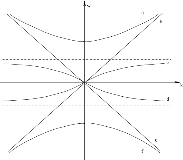
The characteristic variety (that is, the union of the graphs ξ↦λj​(ξ)\xi\mapsto\lambda_{j}(\xi)) is pictured on figure 1. We have that for any ξ∈ℝ\xi\in\mathbb{R}, 1≤j≤6,1\leq j\leq 6, and 7≤j′≤97\leq j^{\prime}\leq 9:

λ1​(ξ)≥2,λ2​(ξ)≥0,0≤λ3​(ξ)<1,λj​(ξ)=−λ7−j​(ξ),λj′​(ξ)=0.\lambda_{1}(\xi)\geq 2,\hskip 8.50012pt\lambda_{2}(\xi)\geq 0,\hskip 8.50012pt0\leq\lambda_{3}(\xi)<1,\hskip 8.50012pt\lambda_{j}(\xi)=-\lambda_{7-j}(\xi),\hskip 8.50012pt\lambda_{j^{\prime}}(\xi)=0. (3.2)

For 1≤j≤61\leq j\leq 6, we have the dispersion relations

ξ2=λj​(ξ)+2​δjλj​(ξ)+δj​λj2​(ξ),δj=(−1)j.\xi^{2}=\frac{\lambda_{j}(\xi)+2\delta_{j}}{\lambda_{j}(\xi)+\delta_{j}}\lambda_{j}^{2}(\xi),\hskip 8.50012pt\delta_{j}=(-1)^{j}. (3.3)
Refer to caption
Figure 1: The characteristic variety.

In order to reveal the Maxwell-Bloch structure, we define

V0=Π0​V=∑j=16Πj​(ε​𝒟y+k​𝒟θ)​V,Vs=Πs​V=∑j=79Πj​(ε​𝒟y+k​𝒟θ)​V,V_{0}=\Pi_{0}V=\sum_{j=1}^{6}\Pi_{j}(\varepsilon{\cal D}_{y}+k{\cal D}_{\theta})V,\hskip 8.50012ptV_{s}=\Pi_{s}V=\sum_{j=7}^{9}\Pi_{j}(\varepsilon{\cal D}_{y}+k{\cal D}_{\theta})V, (3.4)

where the total projectors Π0\Pi_{0} and Πs\Pi_{s} are defined in (1.28) and the notation 𝒟:=∂/i.{\cal D}:=\partial/i. By (1.29), the projector Π0\Pi_{0} and Πs\Pi_{s} are actually constant matrices. By equation (1.11) in VV, the system in (V0,Vs)(V_{0},V_{s}) is

{∂tV0+iε​𝒜0​V0−ω∂θε​V0=Π0​B​(V0+Vs,V0+Vs),∂tVs−ω∂θε​Vs=Πs​B​(V0+Vs,V0+Vs),\left\{\begin{aligned} &\partial_{t}V_{0}+\frac{i}{\varepsilon}\mathcal{A}_{0}V_{0}-\frac{\omega\partial_{\theta}}{\varepsilon}V_{0}=\Pi_{0}B(V_{0}+V_{s},V_{0}+V_{s}),\\ &\partial_{t}V_{s}-\frac{\omega\partial_{\theta}}{\varepsilon}V_{s}=\Pi_{s}B(V_{0}+V_{s},V_{0}+V_{s}),\\ \end{aligned}\right. (3.5)

where the Fourier multiplier

𝒜0=∑j=16λj​(ε​𝒟y+k​𝒟θ)​Πj​(ε​𝒟y+k​𝒟θ).\mathcal{A}_{0}=\sum_{j=1}^{6}\lambda_{j}(\varepsilon{\cal D}_{y}+k{\cal D}_{\theta})\Pi_{j}(\varepsilon{\cal D}_{y}+k{\cal D}_{\theta}). (3.6)

By (1.6) and (1.29), we have

Π0​B​(Π0,Π0)=Π0​B​(Πs,Πs)=Πs​B​(Πs,Πs)=Πs​B​(Π0,Πs)=0.\Pi_{0}B(\Pi_{0},\Pi_{0})=\Pi_{0}B(\Pi_{s},\Pi_{s})=\Pi_{s}B(\Pi_{s},\Pi_{s})=\Pi_{s}B(\Pi_{0},\Pi_{s})=0. (3.7)

Then the equation (3.5) becomes

{∂tV0+iε​𝒜0​V0−ω∂θε​V0=2​Π0​B​(V0,Vs),∂tVs−ω∂θε​Vs=Πs​B​(V0,V0).\left\{\begin{aligned} &\partial_{t}V_{0}+\frac{i}{\varepsilon}\mathcal{A}_{0}V_{0}-\frac{\omega\partial_{\theta}}{\varepsilon}V_{0}=2\Pi_{0}B(V_{0},V_{s}),\\ &\partial_{t}V_{s}-\frac{\omega\partial_{\theta}}{\varepsilon}V_{s}=\Pi_{s}B(V_{0},V_{0}).\\ \end{aligned}\right. (3.8)

3.2 Strong transparency and normal form reduction

The following proposition states that the system (3.8) satisfies a strong transparency hypothesis.

Proposition 3.1.

There exists a constant C>0C>0 such that for all ξ,η∈ℝ\xi,\eta\in\mathbb{R}, for any eigenvalues λj​(ξ),λj′​(η),1≤j,j′≤6\lambda_{j}(\xi),~\lambda_{j^{\prime}}(\eta),1\leq j,j^{\prime}\leq 6, and for all u,v∈ℂ9u,~v\in\mathbb{C}^{9}, one has

|Πs​B​(Πj​(ξ)​u,Πj′​(η)​v)|≤C​|λj​(ξ)+λj′​(η)​‖u‖​v|.|\Pi_{s}B(\Pi_{j}(\xi)u,\Pi_{j^{\prime}}(\eta)v)|\leq C|\lambda_{j}(\xi)+\lambda_{j^{\prime}}(\eta)||u||v|. (3.9)
Proof.

By direct calculation, for any 1≤j≤61\leq j\leq 6, the eigenprojector Πj\Pi_{j} has the formula

Πj(ξ)=1|Qj|2(⋅|Qj(ξ))Qj(ξ),\Pi_{j}(\xi)=\frac{1}{|Q_{j}|^{2}}(~\cdot~|Q_{j}(\xi))Q_{j}(\xi), (3.10)

where

Qj=(−i​δj​ξλj​ΩjΩj−γj​Ωj),Ωj=(0i​δj1),γj=1−ξ2λj2,δj=(−1)j,Q_{j}=\begin{pmatrix}\frac{-i\delta_{j}\xi}{\lambda_{j}}\Omega_{j}\\ \Omega_{j}\\ -\gamma_{j}\Omega_{j}\end{pmatrix},~~\Omega_{j}=\begin{pmatrix}0\\ i\delta_{j}\\ 1\end{pmatrix},~~\gamma_{j}=1-\frac{\xi^{2}}{\lambda_{j}^{2}},~\delta_{j}=(-1)^{j}, (3.11)

and the couple (λj,ξ)(\lambda_{j},\xi) satisfies the dispersion relation (3.3). We then compute

Πs​B​(Qj​(ξ),Qj′​(η))=i2​(γj​(ξ)−γj′​(η)​(δj−δj′)​(0−e1e1)CLOSE.\Pi_{s}B(Q_{j}(\xi),Q_{j^{\prime}}(\eta))=\frac{i}{2}(\gamma_{j}(\xi)-\gamma_{j^{\prime}}(\eta)(\delta_{j}-\delta_{j^{\prime}})\begin{pmatrix}0\\ -e_{1}\\ e_{1}\end{pmatrix}. (3.12)

By (3.11), we have

γj​(ξ)−γj′​(η)\displaystyle\gamma_{j}(\xi)-\gamma_{j^{\prime}}(\eta) =\displaystyle= (1−ξ2λj​(ξ))−(1−η2λj′​(η))\displaystyle(1-\frac{\xi^{2}}{\lambda_{j}(\xi)})-(1-\frac{\eta^{2}}{\lambda_{j^{\prime}}(\eta)}) (3.13)
=\displaystyle= (1−λj​(ξ)+2​δjλj​(ξ)+δj)−(1−λj′​(η)+2​δj′λj′​(η)+δj′)\displaystyle(1-\frac{\lambda_{j}(\xi)+2\delta_{j}}{\lambda_{j}(\xi)+\delta_{j}})-(1-\frac{\lambda_{j^{\prime}}(\eta)+2\delta_{j^{\prime}}}{\lambda_{j^{\prime}}(\eta)+\delta_{j^{\prime}}})
=\displaystyle= −δj​(λj′​(η)−δj​δj′​λj​(ξ))(λj​(ξ)+δj)​(λj′​(η)+δj′).\displaystyle\frac{-\delta_{j}(\lambda_{j^{\prime}}(\eta)-\delta_{j}\delta_{j^{\prime}}\lambda_{j}(\xi))}{(\lambda_{j}(\xi)+\delta_{j})(\lambda_{j^{\prime}}(\eta)+\delta_{j^{\prime}})}.

Recall that δj\delta_{j} and δj′\delta_{j^{\prime}} can only take the value 11 or −1-1. If δj′\delta_{j^{\prime}} and δj\delta_{j} have the same sign, by (3.12), we have Πs​B​(Qj​(ξ),Qj′​(η))=0\Pi_{s}B(Q_{j}(\xi),Q_{j^{\prime}}(\eta))=0; if δj′\delta_{j^{\prime}} and δj\delta_{j} have the opposite sign, by (3.13), we have

Πs​B​(Qj​(ξ),Qj′​(η))=i⁡(λj′+λj)(λj+δj)​(λj′+δj′)​(0−e1e1).\Pi_{s}B(Q_{j}(\xi),Q_{j^{\prime}}(\eta))=\frac{i(\lambda_{j^{\prime}}+\lambda_{j})}{(\lambda_{j}+\delta_{j})(\lambda_{j^{\prime}}+\delta_{j^{\prime}})}\begin{pmatrix}0\\ -e_{1}\\ e_{1}\end{pmatrix}. (3.14)

By (3.10) and direct calculation, the equation (3.9) follows. ∎

With (3.8) and Proposition 3.1, we see that system 3.8 has the Maxwell-Bloch structure (terminology introduced in Section 1.1.2). This allows to use a nonlinear change of variable introduced by Joly, Métivier and Rauch [4]. Together with the preparation condition Πs​V​(0)=O⁡(ε)\Pi_{s}V(0)=O(\varepsilon), this gives existence in time O⁡(1/ε)O(1/\varepsilon) for the solution to the Cauchy problem (3.8). First, changing variable Vs=ε​WsV_{s}=\varepsilon W_{s} gives

{∂tV0+iε​𝒜0​V0−ω∂θε​V0=2​ε​Π0​B​(V0,Ws),∂tWs−ω∂θε​Ws=1ε​Πs​B​(V0,V0).\left\{\begin{aligned} &\partial_{t}V_{0}+\frac{i}{\varepsilon}\mathcal{A}_{0}V_{0}-\frac{\omega\partial_{\theta}}{\varepsilon}V_{0}=2\varepsilon\Pi_{0}B(V_{0},W_{s}),\\ &\partial_{t}W_{s}-\frac{\omega\partial_{\theta}}{\varepsilon}W_{s}=\frac{1}{\varepsilon}\Pi_{s}B(V_{0},V_{0}).\\ \end{aligned}\right. (3.15)

Then we introduce the nonlinear change of variable

N=Ws−J⁡(V0,V0),N=W_{s}-J(V_{0},V_{0}), (3.16)

where the symmetric bilinear form JJ has the following form

J⁡(∑p∈ℤup​ei​p​θ,∑q∈ℤvq​ei​q​θ)=∑p,qJp​q​(up,vq)​ei⁡(p+q)​θ,J(\sum_{p\in\mathbb{Z}}u_{p}e^{ip\theta},\sum_{q\in\mathbb{Z}}v_{q}e^{iq\theta})=\sum_{p,q}J_{pq}(u_{p},v_{q})e^{i(p+q)\theta}, (3.17)

for some Jp​qJ_{pq} to be determined below. The equation in NN is

∂tN−ω∂θε​N=∂tWs−ω∂θε​Ws−J⁡(∂tV0−ω∂θε​V0,V0)−J⁡(V0,∂tV0−ω∂θε​V0)\displaystyle\partial_{t}N-\frac{\omega\partial_{\theta}}{\varepsilon}N=\partial_{t}W_{s}-\frac{\omega\partial_{\theta}}{\varepsilon}W_{s}-J(\partial_{t}V_{0}-\frac{\omega\partial_{\theta}}{\varepsilon}V_{0},V_{0})-J\big(V_{0},\partial_{t}V_{0}-\frac{\omega\partial_{\theta}}{\varepsilon}V_{0}\big)
=1εΠsB(V0,V0)−J(−iε∑j=16λj(ε𝒟y+k𝒟θ)Πj(ε𝒟y+k𝒟θ)V0,V0)\displaystyle~~~=\frac{1}{\varepsilon}\Pi_{s}B(V_{0},V_{0})-J\big(-\frac{i}{\varepsilon}\sum_{j=1}^{6}\lambda_{j}(\varepsilon{\cal D}_{y}+k{\cal D}_{\theta})\Pi_{j}(\varepsilon{\cal D}_{y}+k{\cal D}_{\theta})V_{0},V_{0}\big)
−J(V0,−iε∑j=16λj(ε𝒟y+k𝒟θ)Πj(ε𝒟y+k𝒟θ)V0)−2J(2εΠ0B(V0,Ws),V0).\displaystyle~~~~~~-J\big(V_{0},-\frac{i}{\varepsilon}\sum_{j=1}^{6}\lambda_{j}(\varepsilon{\cal D}_{y}+k{\cal D}_{\theta})\Pi_{j}(\varepsilon{\cal D}_{y}+k{\cal D}_{\theta})V_{0}\big)\ -2J\big(2\varepsilon\Pi_{0}B(V_{0},W_{s}),V_{0}\big).

We choose the bilinear operator JJ to eliminate the singular term of order O⁡(1/ε)O(1/\varepsilon) in the above equation. We consider the following equation

Πs​B​(V0,V0)=−i​J​(∑j=16λj​(ε​𝒟y+k​𝒟θ)​Πj​(ε​𝒟y+k​𝒟θ)​V0,V0)\displaystyle\Pi_{s}B(V_{0},V_{0})=-iJ\big(\sum_{j=1}^{6}\lambda_{j}(\varepsilon{\cal D}_{y}+k{\cal D}_{\theta})\Pi_{j}(\varepsilon{\cal D}_{y}+k{\cal D}_{\theta})V_{0},V_{0}\big)
−i​J​(V0,∑j=16λj​(ε​𝒟y+k​𝒟θ)​Πj​(ε​𝒟y+k​𝒟θ)​V0).\displaystyle~~~~~~~~~~~~~~~~~~~-iJ\big(V_{0},\sum_{j=1}^{6}\lambda_{j}(\varepsilon{\cal D}_{y}+k{\cal D}_{\theta})\Pi_{j}(\varepsilon{\cal D}_{y}+k{\cal D}_{\theta})V_{0}\big).

Equivalently, in Fourier, for all (ξ,η,p,q,j,j′\xi,\eta,p,q,j,j^{\prime}):

Πs​B​(Πj​(ε​η+k​p)​V0​p,Πj′​(ε⁡(ξ−η)+k​q)​V0​q)\displaystyle\Pi_{s}B\big(\Pi_{j}(\varepsilon\eta+kp)V_{0p},\Pi_{j^{\prime}}(\varepsilon(\xi-\eta)+kq)V_{0q}\big)
=−i​λj​(ε​η+k​p)​Jp​q​(Πj​(ε​η+k​p)​V0​p,Πj′​(ε⁡(ξ−η)+k​q)​V0​q)\displaystyle~~~~~~~~~~~~~~~~=-i\lambda_{j}(\varepsilon\eta+kp)J_{pq}\big(\Pi_{j}(\varepsilon\eta+kp)V_{0p},\Pi_{j^{\prime}}(\varepsilon(\xi-\eta)+kq)V_{0q}\big)
−i​λj​(ε⁡(ξ−η)+k​q)​Jp​q​(Πj​(ε​η+k​p)​V0​p,Πj′​(ε⁡(ξ−η)+k​q)​V0​q).\displaystyle~~~~~~~~~~~~~~~~~~~-i\lambda_{j}\big(\varepsilon(\xi-\eta)+kq\big)J_{pq}\big(\Pi_{j}(\varepsilon\eta+kp)V_{0p},\Pi_{j^{\prime}}\big(\varepsilon(\xi-\eta)+kq\big)V_{0q}\big).

A solution to the above equation is given by

Jp​q​(Πj​(ξ)​a,Πj′​(η)​b):=i​∑j=16∑j′=16Πs​B​(Πj​(ξ)​a,Πj′​(η)​b)λj​(ξ)+λj′​(η),for all a,b∈ℂ9.J_{pq}\big(\Pi_{j}(\xi)a,\Pi_{j^{\prime}}(\eta)b\big):=i\sum_{j=1}^{6}\sum_{j^{\prime}=1}^{6}\frac{\Pi_{s}B(\Pi_{j}(\xi)a,\Pi_{j^{\prime}}(\eta)b)}{\lambda_{j}(\xi)+\lambda_{j^{\prime}}(\eta)},~\mbox{for all $a,b\in\mathbb{C}^{9}$}. (3.18)

By Proposition 3.1, JJ is well defined and is bounded from Hs1​(𝕋θ,Hys2)×Hs1​(𝕋θ,Hys2)H^{s_{1}}(\mathbb{T}_{\theta},H^{s_{2}}_{y})\times H^{s_{1}}(\mathbb{T}_{\theta},H^{s_{2}}_{y}) to Hs1​(𝕋θ,Hys2)H^{s_{1}}(\mathbb{T}_{\theta},H^{s_{2}}_{y}) provided s1>1/2,s2>1/2s_{1}>1/2,s_{2}>1/2. The system in (V0,N)(V_{0},N) is now

{∂tV0+iε​𝒜0​V0−ω∂θε​V0=2​ε​Π0​B​(V0,N+J⁡(V0,V0)),∂tN−ω∂θε​N=−2​ε​J​(Π0​B​(V0,N+J⁡(V0,V0)),V0).\left\{\begin{aligned} &\partial_{t}V_{0}+\frac{i}{\varepsilon}\mathcal{A}_{0}V_{0}-\frac{\omega\partial_{\theta}}{\varepsilon}V_{0}=2\varepsilon\Pi_{0}B(V_{0},N+J(V_{0},V_{0})),\\ &\partial_{t}N-\frac{\omega\partial_{\theta}}{\varepsilon}N=-2\varepsilon J(\Pi_{0}B(V_{0},N+J(V_{0},V_{0})),V_{0}).\\ \end{aligned}\right. (3.19)

We then rescale the time and define (𝒱0,𝒩)​(τ,y,θ)=(V0,N)​(τ/ε,y,θ){\displaystyle(\mathcal{V}_{0},\mathcal{N})(\tau,y,\theta)=(V_{0},N)(\tau/\varepsilon,y,\theta)}. The system in (𝒱0,𝒩)(\mathcal{V}_{0},\mathcal{N}) is

{∂τ𝒱0+iε2​𝒜0​𝒱0−ω∂θε2​𝒱0=2​Π0​B​(𝒱0,𝒩+J⁡(𝒱0,𝒱0)),∂τ𝒩−ω∂θε2​𝒩=−2​J​(Π0​B​(𝒱0,𝒩+J⁡(𝒱0,𝒱0)),𝒱0).\left\{\begin{aligned} &\partial_{\tau}\mathcal{V}_{0}+\frac{i}{\varepsilon^{2}}\mathcal{A}_{0}\mathcal{V}_{0}-\frac{\omega\partial_{\theta}}{\varepsilon^{2}}\mathcal{V}_{0}=2\Pi_{0}B(\mathcal{V}_{0},\mathcal{N}+J(\mathcal{V}_{0},\mathcal{V}_{0})),\\ &\partial_{\tau}\mathcal{N}-\frac{\omega\partial_{\theta}}{\varepsilon^{2}}\mathcal{N}=-2J(\Pi_{0}B(\mathcal{V}_{0},\mathcal{N}+J(\mathcal{V}_{0},\mathcal{V}_{0})),\mathcal{V}_{0}).\\ \end{aligned}\right. (3.20)

The initial datum is

{𝒱0​(0,y,θ)=Π0​V​(0,y,θ)=Π0​(ei​θ​a​(y)+e−i​θ​a⁡(y)¯+ε​a1​(y,θ)+ε2​a2​(y,θ)),𝒩⁡(0,y,θ)=Ws​(0,y,θ)−J⁡(𝒱0,𝒱0)​(0,y,θ)=1ε​Πs​V​(0,y,θ)−J⁡(𝒱0,𝒱0)​(0,y,θ).\left\{\begin{aligned} &\mathcal{V}_{0}(0,y,\theta)=\Pi_{0}V(0,y,\theta)=\Pi_{0}(e^{i\theta}a(y)+e^{-i\theta}\overline{a(y)}+\varepsilon a_{1}(y,\theta)+\varepsilon^{2}a_{2}(y,\theta)),\\ &\mathcal{N}(0,y,\theta)=W_{s}(0,y,\theta)-J(\mathcal{V}_{0},\mathcal{V}_{0})(0,y,\theta)=\frac{1}{\varepsilon}\Pi_{s}V(0,y,\theta)-J(\mathcal{V}_{0},\mathcal{V}_{0})(0,y,\theta).\end{aligned}\right. (3.21)

Since the leading term a⁡(y)a(y) belongs to ker⁡L⁡(i⁡(ω,k))\ker L(i(\omega,k)), and ω≠0\omega\neq 0, we have Πs​a=0\Pi_{s}a=0. Then the initial datum for 𝒩\mathcal{N} is O⁡(1)O(1) in H1​(𝕋θ,Hys−2)H^{1}(\mathbb{T}_{\theta},H^{s-2}_{y}):

𝒩⁡(0,y,θ)=Πs​a1​(y,θ)+ε​Πs​a2​(y,θ)−J⁡(𝒱0,𝒱0)​(0,y,θ)∈H1​(𝕋θ,Hys−2).\mathcal{N}(0,y,\theta)=\Pi_{s}a_{1}(y,\theta)+\varepsilon\Pi_{s}a_{2}(y,\theta)-J(\mathcal{V}_{0},\mathcal{V}_{0})(0,y,\theta)\in H^{1}(\mathbb{T}_{\theta},H^{s-2}_{y}).

This gives well-posedness over diffractive times:

Proposition 3.2.

The Cauchy problem (3.20)-(3.21) admits a unique solution on a time interval [0,T2∗[[0,T_{2}^{*}[, with T2∗>0T_{2}^{*}>0 independent of ε\varepsilon. Moreover, for all T<T2∗T<T_{2}^{*}, we have the estimates :

sup[0,T]‖(𝒱0,𝒩)​(τ)‖H1​(𝕋θ,Hys−2)≤C,\sup_{[0,T]}\|(\mathcal{V}_{0},\mathcal{N})(\tau)\|_{H^{1}(\mathbb{T}_{\theta},H^{s-2}_{y})}\leq C,

where the constant C=C⁡(s,T)C=C(s,T) is independent of ε\varepsilon and depends on ss through the sum of norms ‖a‖Hys+‖a1‖H1​(𝕋θ,Hys−1)+‖a2‖H1​(𝕋θ,Hys−2).\|a\|_{H^{s}_{y}}+\|a_{1}\|_{H^{1}(\mathbb{T}_{\theta},H^{s-1}_{y})}+\|a_{2}\|_{H^{1}(\mathbb{T}_{\theta},H^{s-2}_{y})}.

Proof.

The system (3.20) being symmetric hyperbolic, local-in-time well-posedness is classical. Here the bounds are uniform in ε\varepsilon. Indeed, the initial datum (3.21) is uniformly bounded with respect to ε\varepsilon in Sobolev spaces H1​(𝕋θ,Hys−2),s>2+1/2H^{1}(\mathbb{T}_{\theta},H^{s-2}_{y}),~s>2+1/2. The L2L^{2} estimate is uniform in ε\varepsilon in spite of the large 1/ε1/\varepsilon prefactor because the operator −ω∂θ+A(e1)k∂θ+L0-\omega\partial_{\theta}+A(e_{1})k\partial_{\theta}+L_{0} is skew-adjoint, and the commutator estimates are trivial because the operator −ω∂θ+A(e1)k∂θ+L0-\omega\partial_{\theta}+A(e_{1})k\partial_{\theta}+L_{0} has constant coefficients. ∎

Back to the variable (V0,N)(V_{0},N), where V0V_{0} and NN are introduced in (3.4) and (3.16) respectively, by the definition of (𝒱0,𝒩)(\mathcal{V}_{0},\mathcal{N}), we have that (V0,N)(V_{0},N) is well defined over the long time interval [0,T2∗/ε[[0,T_{2}^{*}/\varepsilon[. Back to the variable VV introduced in (1.10), this gives well-posedness over the time interval [0,T2∗/ε[[0,T_{2}^{*}/\varepsilon[ with the estimates for any T<T2∗T<T_{2}^{*}:

sup[0,T/ε]‖Π0​V​(t)‖H1​(𝕋θ,Hys−2)≤C,sup[0,T/ε]‖Πs​V​(t)‖H1​(𝕋θ,Hys−2)≤C​ε,\sup_{[0,T/\varepsilon]}\|\Pi_{0}V(t)\|_{H^{1}(\mathbb{T}_{\theta},H^{s-2}_{y})}\leq C,~~\sup_{[0,T/\varepsilon]}\|\Pi_{s}V(t)\|_{H^{1}(\mathbb{T}_{\theta},H^{s-2}_{y})}\leq C\varepsilon, (3.22)

for the same constant C=C⁡(s,T)C=C(s,T) as in Proposition 3.2.

We proved the long time existence of order O⁡(1/ε)O(1/\varepsilon) of the solution of the Cauchy problem (1.20). Back to the original variable v⁡(t,y)=V⁡(t,y,θ)|θ=−ω​t+k​yε{\displaystyle v(t,y)=V(t,y,\theta)|_{\theta=\frac{-\omega t+ky}{\varepsilon}}}, the following corollary follows immediately.

Corollary 3.3.

Over the time interval [0,T2∗/ε[[0,T_{2}^{*}/\varepsilon[, the Cauchy problem (1.7)-(1.9) admits a unique solution vv of the form v⁡(t,x)=V⁡(t,x,k​y−ω​tε){\displaystyle v(t,x)=V(t,x,\frac{ky-\omega t}{\varepsilon})}, with V⁡(t,x,θ)∈L∞​([0,T/ε]t,H1​(𝕋θ,Hs−2​(ℝy1)))V(t,x,\theta)\in L^{\infty}([0,T/\varepsilon]_{t},H^{1}(\mathbb{T}_{\theta},H^{s-2}(\mathbb{R}^{1}_{y}))) for any T<T2∗T<T_{2}^{*}. Moreover, by Sobolev embedding, we have |v|L∞≤C|v|_{L^{\infty}}\leq C, where C=C⁡(s,T)C=C(s,T) is given in Proposition 3.2.

In the next section, we consider the stability of the WKB solution from Section 2 and show two convergence results.

4 Error estimates

For the WKB solution VaV^{a} from Section 2, we use the projection, rescalling and normal form reduction from Section 3:

(V0a,Vsa)=(Π0​Va,Πs​Va),Wsa=Vsaε,Na=Wsa−J⁡(V0a,V0a),(𝒱0a,𝒩a)​(τ)=(V0a,Na)​(τ/ε).(V^{a}_{0},V^{a}_{s})=(\Pi_{0}V^{a},\Pi_{s}V^{a}),\hskip 8.50012ptW^{a}_{s}=\frac{V^{a}_{s}}{\varepsilon},\hskip 8.50012ptN^{a}=W^{a}_{s}-J(V^{a}_{0},V^{a}_{0}),\hskip 8.50012pt(\mathcal{V}^{a}_{0},\mathcal{N}^{a})(\tau)=(V^{a}_{0},N^{a})(\tau/\varepsilon).

where JJ is defined by (3.17) and (3.18). Then the system in (𝒱0a,𝒩a)(\mathcal{V}^{a}_{0},\mathcal{N}^{a}) is

{∂τ𝒱0a+iε2​𝒜0​𝒱0a−ω∂θε2​V0a=2​Π0​B​(𝒱0a,𝒩a+J⁡(𝒱0a,𝒱0a))+ε​Π0​R,∂τ𝒩a−ω∂θε2​𝒩a=−2​J​(Π0​B​(𝒱0a,𝒩a+J⁡(𝒱0a,𝒱0a)),𝒱0a)−2​ε​J​(𝒱0a,Π0​R)+Πs​R\left\{\begin{aligned} &\partial_{\tau}\mathcal{V}^{a}_{0}+\frac{i}{\varepsilon^{2}}\mathcal{A}_{0}\mathcal{V}^{a}_{0}-\frac{\omega\partial_{\theta}}{\varepsilon^{2}}V^{a}_{0}=2\Pi_{0}B(\mathcal{V}^{a}_{0},\mathcal{N}^{a}+J(\mathcal{V}^{a}_{0},\mathcal{V}^{a}_{0}))+\varepsilon\Pi_{0}R,\\ &\partial_{\tau}\mathcal{N}^{a}-\frac{\omega\partial_{\theta}}{\varepsilon^{2}}\mathcal{N}^{a}=-2J(\Pi_{0}B(\mathcal{V}^{a}_{0},\mathcal{N}^{a}+J(\mathcal{V}^{a}_{0},\mathcal{V}^{a}_{0})),\mathcal{V}^{a}_{0})-2\varepsilon J(\mathcal{V}_{0}^{a},\Pi_{0}R)+\Pi_{s}R\\ \end{aligned}\right. (4.1)

As shown in Section 2.2, an existence time for (4.1) is T1∗T^{*}_{1} (introduced in Section 2 as an existence time for (2.41)). Define the perturbations

Φ⁡(τ,y,θ)=(𝒱0−𝒱0a)​(τ,y,θ),Ψ⁡(τ,y,θ)=(𝒩−𝒩a)​(τ,y,θ),\Phi(\tau,y,\theta)=(\mathcal{V}_{0}-\mathcal{V}_{0}^{a})(\tau,y,\theta),~~\Psi(\tau,y,\theta)=(\mathcal{N}-\mathcal{N}^{a})(\tau,y,\theta), (4.2)

then the couple (Φ,Ψ\Phi,\Psi) solves the following system over time interval [0,T12∗[[0,T_{12}^{*}[~ with T12∗=min⁡{T1∗,T2∗}T_{12}^{*}=\min\{T_{1}^{*},T_{2}^{*}\} (T2∗T_{2}^{*} is introduced in Proposition 3.2 as an existence time of (𝒱0,𝒩)(\mathcal{V}_{0},\mathcal{N}) for (3.20)-(3.21)):

{∂τΦ+iε2​𝒜0​Φ−ω∂θε2​Φ=2​Π0​B​(𝒱0a,Ψ)+H0​(𝒱0a,𝒩a,Φ,Ψ)−ε​Π0​R,∂τΨ−ω∂θε2​Ψ=Hs​(𝒱0a,𝒩,Φ,Ψ)+2​ε​J​(𝒱0a,Π0​R)−Πs​R,\left\{\begin{aligned} &\partial_{\tau}\Phi+\frac{i}{\varepsilon^{2}}\mathcal{A}_{0}\Phi-\frac{\omega\partial_{\theta}}{\varepsilon^{2}}\Phi=2\Pi_{0}B(\mathcal{V}^{a}_{0},\Psi)+H_{0}(\mathcal{V}^{a}_{0},\mathcal{N}^{a},\Phi,\Psi)-\varepsilon\Pi_{0}R,\\ &\partial_{\tau}\Psi-\frac{\omega\partial_{\theta}}{\varepsilon^{2}}\Psi=H_{s}(\mathcal{V}^{a}_{0},\mathcal{N},\Phi,\Psi)+2\varepsilon J(\mathcal{V}_{0}^{a},\Pi_{0}R)-\Pi_{s}R,\\ \end{aligned}\right. (4.3)

where H0H_{0} and HsH_{s} are defined by

{H0​(𝒱0a,𝒩a,Φ,Ψ):=2​Π0​B​(Φ,𝒩a+Ψ+J⁡(𝒱0a+Φ,𝒱0a+Φ))+2​Π0​B​(𝒱0a,J⁡(Φ,Φ+2​𝒱0a)),Hs​(𝒱0a,𝒩a,Φ,Ψ):=2​J​(Π0​B​(𝒱0a,𝒩a+J⁡(𝒱0a,𝒱0a)),𝒱0a)−2​J​(Π0​B​(𝒱0a+Φ,𝒩a+Ψ+J⁡(𝒱0a+Φ,𝒱0a+Φ)),𝒱0a+Φ).\left\{\begin{aligned} &H_{0}(\mathcal{V}^{a}_{0},\mathcal{N}^{a},\Phi,\Psi):=2\Pi_{0}B(\Phi,\mathcal{N}^{a}+\Psi+J(\mathcal{V}_{0}^{a}+\Phi,\mathcal{V}_{0}^{a}+\Phi))+2\Pi_{0}B(\mathcal{V}^{a}_{0},J(\Phi,\Phi+2\mathcal{V}^{a}_{0})),\\ &\begin{split}H_{s}(\mathcal{V}^{a}_{0},\mathcal{N}^{a},\Phi,\Psi):=&2J(\Pi_{0}B(\mathcal{V}^{a}_{0},\mathcal{N}^{a}+J(\mathcal{V}^{a}_{0},\mathcal{V}^{a}_{0})),\mathcal{V}^{a}_{0})\\ &\hskip 8.50012pt-2J(\Pi_{0}B(\mathcal{V}_{0}^{a}+\Phi,\mathcal{N}^{a}+\Psi+J(\mathcal{V}_{0}^{a}+\Phi,\mathcal{V}_{0}^{a}+\Phi)),\mathcal{V}^{a}_{0}+\Phi).\end{split}\\ \end{aligned}\right. (4.4)

By (2.46), the initial datum for (Φ,Ψ\Phi,\Psi) is

{Φ⁡(0)=(V0−V0a)​(0)=−ε​Π0​b−ε2​Π0​b1,Ψ⁡(0)=1ε​(Vs−Vsa)​(0)−J⁡(V0,V0)​(0)+J⁡(Va,Va)​(0)=−Πs​b+ε​b2,\left\{\begin{aligned} &\Phi(0)=(V_{0}-V_{0}^{a})(0)=-\varepsilon\Pi_{0}b-\varepsilon^{2}\Pi_{0}b_{1},\\ &\Psi(0)=\frac{1}{\varepsilon}(V_{s}-V_{s}^{a})(0)-J(V_{0},V_{0})(0)+J(V^{a},V^{a})(0)=-\Pi_{s}b+\varepsilon b_{2},\\ \end{aligned}\right. (4.5)

where bb and b1b_{1} are defined by (2.47) and (2.48), and b2∈H1​(𝕋θ,Hys−2)b_{2}\in H^{1}(\mathbb{T}_{\theta},H^{s-2}_{y}) is defined by

b2=−Πs​b1+J⁡(b+ε​b1,Va​(0))+J⁡(V⁡(0),b+ε​b1).b_{2}=-\Pi_{s}b_{1}+J(b+\varepsilon b_{1},V_{a}(0))+J(V(0),b+\varepsilon b_{1}).

We give two estimates for (Φ,Ψ\Phi,\Psi) in the following two sections.

4.1 First error estimate

Here we assume only the polarization condition a⁡(y)∈ker⁡L⁡(i⁡(ω,k))a(y)\in\ker L(i(\omega,k)). Then by (4.9), we have Φ⁡(0)=O⁡(ε),Ψ⁡(0)=O⁡(1)\Phi(0)=O(\varepsilon),~\Psi(0)=O(1) in H1​(𝕋θ,Hys−2)H^{1}(\mathbb{T}_{\theta},H^{s-2}_{y}). Then for the symmetric hyperbolic system (4.3), we have the following proposition:

Proposition 4.1.

The Cauchy problem (4.3)-(4.9) admits a unique solution on time interval [0,T3∗[[0,T_{3}^{*}[ with T3∗≥T12∗T_{3}^{*}\geq T_{12}^{*}, and the following estimates hold for any T<T3∗T<T_{3}^{*}:

‖Φ‖L∞​([0,T],H1​(𝕋θ,Hys−2))≤C⁡(ε+T),‖Ψ‖L∞​([0,T],H1​(𝕋θ,Hys−2))≤C,\|\Phi\|_{L^{\infty}([0,T],H^{1}(\mathbb{T}_{\theta},H^{s-2}_{y}))}\leq C(\varepsilon+T),~~\|\Psi\|_{L^{\infty}([0,T],H^{1}(\mathbb{T}_{\theta},H^{s-2}_{y}))}\leq C,\\ (4.6)

where the constant C=C⁡(s,T)C=C(s,T) is independent of ε\varepsilon and depends on ss through the sum of norms ‖a‖Hys+‖a1‖H1​(𝕋θ,Hys−1)+‖a2‖H1​(𝕋θ,Hys−2).\|a\|_{H^{s}_{y}}+\|a_{1}\|_{H^{1}(\mathbb{T}_{\theta},H^{s-1}_{y})}+\|a_{2}\|_{H^{1}(\mathbb{T}_{\theta},H^{s-2}_{y})}.

Proof.

As in the proof of Proposition 3.2, the data being bounded in ε\varepsilon, we have existence, uniqueness, and uniform bounds in ε\varepsilon for short times with existence time T3∗T^{*}_{3} independent of ε\varepsilon.

The source terms of (4.3) is O⁡(1)O(1), then we have the estimate:

‖(Φ,Ψ)‖L∞​([0,T],H1​(𝕋θ,Hys−2))≤C.\|(\Phi,\Psi)\|_{L^{\infty}([0,T],H^{1}(\mathbb{T}_{\theta},H^{s-2}_{y}))}\leq C. (4.7)

By the first equation of (4.9), the initial datum Φ⁡(0)=O⁡(ε)\Phi(0)=O(\varepsilon). The classical HsH^{s} estimate then gives

‖Φ‖L∞​([0,T],H1​(𝕋θ,Hys−2))≤C⁡(|Φ⁡(0)|L∞​([0,T],H1​(𝕋θ,Hys−2))+∫0TC​𝑑t)≤C⁡(ε+T)\|\Phi\|_{L^{\infty}([0,T],H^{1}(\mathbb{T}_{\theta},H^{s-2}_{y}))}\leq C\big(|\Phi(0)|_{L^{\infty}([0,T],H^{1}(\mathbb{T}_{\theta},H^{s-2}_{y}))}+\int_{0}^{T}C~dt\big)\leq C(\varepsilon+T) (4.8)

Since we already know that (Φ,Ψ\Phi,\Psi) defined by (4.2) solves (4.3)-(4.9) over time interval [0,T12∗[[0,T_{12}^{*}[ where T12∗:=min⁡{T1∗,T2∗}T_{12}^{*}:=\min\{T_{1}^{*},T_{2}^{*}\}, we have T3∗≥T12∗T_{3}^{*}\geq T_{12}^{*} by uniqueness. ∎

Remark 4.2.

Here we show first that the exact solution exists over long times O⁡(1/ε)O(1/\varepsilon) before showing that it is approximated by the WKB solution on the intersection of their intervals of existence. Indeed, the Maxwell-Bloch structure allows us to find the normal form of the nonlinear equations, in contrast to, e.g., the linear normal form reduction of [9].

Remark 4.3.

For this first error estimate, we do not need the special choice of ff given by (2.43). The estimate (4.6), as well as the first estimate (1.24) in Theorem 1.3, hold for any regular function ff that satisfies the transport equation (2.38), e.g. f=0f=0. (Recall, ff is introduced in Section 2.1 as a building block of the first corrector V1V^{1} in WKB approximation. See (2.18)).

Back to the original time and variables, we immediately obtain the following corollary:

Corollary 4.4.

For any T<T12∗T<T_{12}^{*}, we have the error estimate

{‖Π0​(V−Va)‖L∞​([0,T/ε],H1​(𝕋θ,Hys−2))≤C⁡(ε+T),‖Πs​(V−Va)‖L∞​([0,T/ε],H1​(𝕋θ,Hys−2))≤C​ε.\left\{\begin{aligned} \|\Pi_{0}(V-V^{a})\|_{L^{\infty}([0,T/\varepsilon],H^{1}(\mathbb{T}_{\theta},H^{s-2}_{y}))}&\leq C(\varepsilon+T),\\ \|\Pi_{s}(V-V^{a})\|_{L^{\infty}([0,T/\varepsilon],H^{1}(\mathbb{T}_{\theta},H^{s-2}_{y}))}&\leq C\varepsilon.\\ \end{aligned}\right. (4.9)

The constant C=C⁡(s,T)C=C(s,T) is as in Proposition 4.1.

4.2 Second error estimate

In this section, we show the stability of the WKB solution in the following sense: for some T>0T>0 independent of ε\varepsilon, we have

‖Π0​(V−Va)‖L∞​([0,T/ε],H1​(𝕋θ,Hys−2))=O⁡(ε),‖Πs​(V−Va)‖L∞​([0,T/ε],H1​(𝕋θ,Hys−2))=O⁡(ε2),\|\Pi_{0}(V-V^{a})\|_{L^{\infty}([0,T/\varepsilon],H^{1}(\mathbb{T}_{\theta},H^{s-2}_{y}))}=O(\varepsilon),~~\|\Pi_{s}(V-V^{a})\|_{L^{\infty}([0,T/\varepsilon],H^{1}(\mathbb{T}_{\theta},H^{s-2}_{y}))}=O(\varepsilon^{2}),

provided the initial perturbation

‖Π0​(V−Va)​(0)‖H1​(𝕋θ,Hys−2)=O⁡(ε),‖Πs​(V−Va)​(0)‖H1​(𝕋θ,Hys−2)=O⁡(ε2).\|\Pi_{0}(V-V^{a})(0)\|_{H^{1}(\mathbb{T}_{\theta},H^{s-2}_{y})}=O(\varepsilon),~~\|\Pi_{s}(V-V^{a})(0)\|_{H^{1}(\mathbb{T}_{\theta},H^{s-2}_{y})}=O(\varepsilon^{2}). (4.10)

Here we assume that the initial corrector a1a_{1} satisfies (2.51). Then by Lemma (2.1),

‖Πs​(V−Va)‖L∞​([0,T/ε],H1​(𝕋θ,Hys−2))=O⁡(ε2),\|\Pi_{s}(V-V^{a})\|_{L^{\infty}([0,T/\varepsilon],H^{1}(\mathbb{T}_{\theta},H^{s-2}_{y}))}=O(\varepsilon^{2}),

and the initial datum of (Φ,Ψ\Phi,\Psi) (introduced in (4.2)) is

Φ⁡(0)=−ε​Π0​b−ε2​Π0​b1=O⁡(ε),Ψ⁡(0)=−Πs​b+ε​b2=ε​b2=O⁡(ε).\Phi(0)=-\varepsilon\Pi_{0}b-\varepsilon^{2}\Pi_{0}b_{1}=O(\varepsilon),\hskip 8.50012pt\Psi(0)=-\Pi_{s}b+\varepsilon b_{2}=\varepsilon b_{2}=O(\varepsilon). (4.11)

For the remainder RR (introduced in (2.46) and explicitly given in (2.49)), with the choice of ff in (2.43), by Lemma 2.2, we have that Πs​R=−ε​Rs\Pi_{s}R=-\varepsilon R_{s} with Rs=2​B​(V1,V2)+ε​B​(V2,V2)∈L∞​([0,T/ε],H1​(𝕋θ,Hys−2))R_{s}=2B(V^{1},V^{2})+\varepsilon B(V^{2},V^{2})\in L^{\infty}([0,T/\varepsilon],H^{1}(\mathbb{T}_{\theta},H^{s-2}_{y})) for any T<T1∗T<T^{*}_{1}. We now consider the rescaled variables

Φ1=Φ/ε,Ψ1=Ψ/ε,\Phi_{1}=\Phi/\varepsilon,~\Psi_{1}=\Psi/\varepsilon, (4.12)

then the equation in (Φ1,Ψ1\Phi_{1},\Psi_{1}) is

{∂τΦ1+iε2​𝒜0​Φ1−ω∂θε2​Φ1=2​Π0​B​(𝒱0a,Ψ1)+1ε​H0​(𝒱0a,𝒩a,ε​Φ1,ε​Ψ1)−Π0​R,∂τΨ1−ω∂θε2​Ψ1=1ε​Hs​(𝒱0a,𝒩,ε​Φ1,ε​Ψ1)+2​J​(𝒱0a,Π0​R)−Rs,\left\{\begin{aligned} &\partial_{\tau}\Phi_{1}+\frac{i}{\varepsilon^{2}}\mathcal{A}_{0}\Phi_{1}-\frac{\omega\partial_{\theta}}{\varepsilon^{2}}\Phi_{1}=2\Pi_{0}B(\mathcal{V}^{a}_{0},\Psi_{1})+\frac{1}{\varepsilon}H_{0}(\mathcal{V}^{a}_{0},\mathcal{N}^{a},\varepsilon\Phi_{1},\varepsilon\Psi_{1})-\Pi_{0}R,\\ &\partial_{\tau}\Psi_{1}-\frac{\omega\partial_{\theta}}{\varepsilon^{2}}\Psi_{1}=\frac{1}{\varepsilon}H_{s}(\mathcal{V}^{a}_{0},\mathcal{N},\varepsilon\Phi_{1},\varepsilon\Psi_{1})+2J(\mathcal{V}_{0}^{a},\Pi_{0}R)-R_{s},\\ \end{aligned}\right. (4.13)

with the initial datum

Φ1​(0)=−Π0​b−ε​Π0​b1,Ψ1​(0)=b2,\Phi_{1}(0)=-\Pi_{0}b-\varepsilon\Pi_{0}b_{1},\hskip 8.50012pt\Psi_{1}(0)=b_{2}, (4.14)

and where (H0,Hs)(H_{0},H_{s}) are defined in (4.4). Note that by bilinearity of BB, and pointwise bounds for the approximate solution, we have uniform bounds

1ε​|H0​(𝒱0a,𝒩a,ε​Φ,ε​Ψ)|≤C⁡(|Φ|+|Ψ|),1ε​|Hs​(𝒱0a,𝒩a,ε​Φ,ε​Ψ)|≤C⁡(|Φ|+|Ψ|).\frac{1}{\varepsilon}|H_{0}({\cal V}_{0}^{a},{\cal N}^{a},\varepsilon\Phi,\varepsilon\Psi)|\leq C(|\Phi|+|\Psi|),\hskip 17.00024pt\frac{1}{\varepsilon}|H_{s}({\cal V}_{0}^{a},{\cal N}^{a},\varepsilon\Phi,\varepsilon\Psi)|\leq C(|\Phi|+|\Psi|).

It is now classical to deduce uniform bounds for Φ1\Phi_{1} and Ψ1\Psi_{1} in times O⁡(1)O(1):

Proposition 4.5.

With the choice of a1a_{1} in (2.51), the Cauchy problem (4.13)-(4.14) admits a unique solution (Φ1,Ψ1\Phi_{1},\Psi_{1}) on [0,T4∗[[0,T_{4}^{*}[ with T4∗>0T_{4}^{*}>0 independent of ε\varepsilon, and for any T<T4∗T<T_{4}^{*}:

‖Φ1‖L∞​([0,T],H1​(𝕋θ,Hys−2))≤C,‖Ψ1‖L∞​([0,T],H1​(𝕋θ,Hys−2))≤C,\|\Phi_{1}\|_{L^{\infty}([0,T],H^{1}(\mathbb{T}_{\theta},H^{s-2}_{y}))}\leq C,~~\|\Psi_{1}\|_{L^{\infty}([0,T],H^{1}(\mathbb{T}_{\theta},H^{s-2}_{y}))}\leq C,\\ (4.15)

where the constant C=C⁡(s,T)C=C(s,T) is independent of ε\varepsilon and depends on ss through the sum of norms ‖a‖Hys+‖a1‖H1​(𝕋θ,Hys−1)+‖a2‖H1​(𝕋θ,Hys−2).\|a\|_{H^{s}_{y}}+\|a_{1}\|_{H^{1}(\mathbb{T}_{\theta},H^{s-1}_{y})}+\|a_{2}\|_{H^{1}(\mathbb{T}_{\theta},H^{s-2}_{y})}.

Remark 4.6.

For this second error estimate, we do need the special choice of ff in (2.43). Together with the choice of initial corrector a1a_{1} in (2.51), it allows us to rescale the solution (4.12) to obtain the desired estimates.

Back to the original time and variables, we immediately deduce the following corollary:

Corollary 4.7.

Let T∗=min⁡{T12∗,T4∗}T^{*}=\min\{T_{12}^{*},T_{4}^{*}\}, then for any T<T∗T<T^{*}, we have the error estimates

‖Π0​(V−Va)‖L∞​([0,T/ε],H1​(𝕋θ,Hys−2))≤C​ε,‖Πs​(V−Va)‖L∞​([0,T/ε],H1​(𝕋θ,Hys−2))≤C​ε2,\|\Pi_{0}(V-V^{a})\|_{L^{\infty}([0,T/\varepsilon],H^{1}(\mathbb{T}_{\theta},H^{s-2}_{y}))}\leq C\varepsilon,~~\|\Pi_{s}(V-V^{a})\|_{L^{\infty}([0,T/\varepsilon],H^{1}(\mathbb{T}_{\theta},H^{s-2}_{y}))}\leq C\varepsilon^{2}, (4.16)

where the constant C=C⁡(s,T)C=C(s,T) is as in Proposition 4.5.

This shows stability, that is, the WKB approximate profile stays close to the exact profile over its existence time with an error estimate that is comparable to the initial error.

4.3 Proof of Theorem 1.3

We now sum up and prove Theorem 1.3.

First, by Corollary 3.3, the function v⁡(t,y)=V⁡(t,y,θ)|θ=k​y−ω​tεv(t,y)=V(t,y,\theta)|_{\theta=\frac{ky-\omega t}{\varepsilon}} solves (1.7)-(1.9) over time interval [0,T∗[[0,T^{*}[, and this gives the first result of Theorem 1.3.

Second, by the Corollary 4.4 and Sovolev embedding H1​(𝕋θ,Hys−2)⊂L∞​(𝕋θ×ℝy)H^{1}(\mathbb{T}_{\theta},H^{s-2}_{y})\subset L^{\infty}(\mathbb{T}_{\theta}\times\mathbb{R}_{y}), the error estimates (1.24) and (1.26) of Theorem 1.3 follow immediately.

Finally, by the Corollary 4.7 and Sovolev embedding H1​(𝕋θ,Hys−2)⊂L∞​(𝕋θ×ℝy)H^{1}(\mathbb{T}_{\theta},H^{s-2}_{y})\subset L^{\infty}(\mathbb{T}_{\theta}\times\mathbb{R}_{y}), we have the second error estimate (1.25). This shows stability of the approximate solution.

Acknowledgment. I warmly thank Eric Dumas and Isabelle Gallagher for stimulating discussions. I particularly thank my advisor Benjamin Texier for his fruitful remarks and for suggesting this interesting subject.

References

  • [1] T. Colin, Rigorous derivation of the nonlinear Schrödinger equation and Davey-Stewartson systems from quadratic hyperbolic systems, Asymptotic Analysis (2002), 69-91.
  • [2] T. Colin, D. Lannes, Justification of and long-wave correction to Davey-Stewartson systems from quadratic hyperbolic systems, Discrete and Continuous Dynamical Systems, vol. 11, n. 1 (2004), 83-100.
  • [3] J.-L. Joly, G. Métivier, J. Rauch, Dispersive nonlinear geometric optics with rectification, Indiana U. Math. J., vol. 47 (1998), 1167-1241.
  • [4] J.-L. Joly, G. Métivier, J. Rauch, Transparent nonlinear geometric optics and Maxwell-Bloch equations, J. Diff. Eq., vol. 166 (2000), 175-250.
  • [5] D. Lannes, Dispersive effects for nonlinear geometrical optics with rectification, Asymptotic Analysis, vol. 18 (1998), 111–146.
  • [6] D. Lannes, Secular growth estimates for hyperbolic systems, J. Diff. Eq.,vol. 190 (2003), 466–503.
  • [7] H. Leblond, Electromagnetic waves in ferromagnets: a Davey-Stewartson-type model, J. Phys. A: Math. Gen., vol. 32, (1999), 7907–7932.
  • [8] B. Texier, The short wave limit for nonlinear, symmetric hyperbolic systems, Adv. Diff. Eq. 9 (2004), no. 1, 1-52.
  • [9] B. Texier, Derivation of the Zakharov equations, Arch. Rational Mech. Anal vol. 184 (2007), 121–183.