Spatiotemporal heterogeneity of local free volumes in highly supercooled liquid

First, for each particle $i$, we define the local density by counting the particles within the distance $\Delta r=|\bm{r}-\bm{r}_{i}|\leq r_{0}$ from $i$

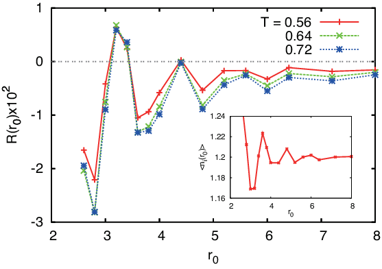
This local density is weighted by the assumed area $\sigma_{j}^{2}$. The inset of Fig. 1 shows the long-time average of the local density $[\overline{n_{i}(r_{0})}]_{N}$ at $T=0.56$. Here, $[\mathcal{A}_{i}]_{N}=N^{-1}\sum_{i}\mathcal{A}_{i}$ denotes the average over all the particles. This quantity corresponds to a radial distribution function $g(r_{0})$ defined in a naive manner.

For the same simulation run, at appropriate time intervals, we estimate the local density in the configuration rearranging regions of dynamical heterogeneity as follows: bonds are defined at each time $t_{0}$ as particle pairs between $i$ and $j$ satisfying the condition[2, 3, 8]

and after a time interval $\Delta t$ bonds are regarded to be broken if

where the cutoffs are set to $A_{1}=1.15$ and $A_{2}=1.6$. Further, in the remainder of this paper, broken bonds in the time interval $[t,t+\Delta t]$ are defined in the same way. We obtain the local density profile only for particles that have undergone bond breakage in a time interval of $\Delta t=2\times 10^{2}$. More precisely, we check whether all the bonds existing at time $t=t_{0}$ are broken after a time interval of $\Delta t$, and for the particles having at least one broken bond the long-time average of the local density $n_{i}$ is calculated. Their average local density profile is denoted as $[n_{i}(r_{0})]_{\rm b.b.}$. The main graph in Fig. 1 shows the long-time average $\overline{R(r_{0},\Delta t)}$ of the relative degree of deviation as given by

While $R(r_{0})$ exhibits an oscillating behavior at small values of $r_{0}$ mainly due to the mixed contributions from larger and smaller components, its value is systematically lower than zero when $r_{0}$ is sufficiently large. Thus, around the broken bonds, i.e., in the configuration rearranging regions, the degree of local density can be characterized with a sufficiently large value of $r_{0}$ at each particle. We employ $r_{0}=6.0$ in our following discussions.

Dynamic heterogeneity is defined as a ubiquitous property of supercooled liquids in which configuration-rearranging regions emerge heterogeneously in the system. This property can be parametrized with various quantities including the van Hove correlation,[5] particle displacements,[4, 39] and four-point correlation functions. Here, to characterize the mobile regions of dynamical heterogeneity, we follow the method of broken bonds[2, 3, 8], in which the number of broken-bond pairs for each particle is counted as $\mathcal{B}_{i}(\Delta t)=\sum_{j\in{\rm b.b.}}1$. Here, the summation is taken over $j$ particles at the broken bond ends of $i$ particles calculated over time intervals of length $\Delta t$, where the definition of broken bond pairs is given by Eqs. (2) and (3). The broken bond distribution is a representation of irreversible configuration rearrangements, where collective motion due to long-wavelength sound modes is eliminated. To illustrate the irreversibility of the bond breakage, in Fig. 3, the total number of the remaining bonds $N_{b}(t)$[8] is plotted for $T=0.64$, which is the number of unbroken bonds for the same thresholds $A_{1}$ and $A_{2}$. Several pairs of particles $i,j$ satisfying Eq. (2) at time $t=0$ approach their counterparts again at time $t^{\prime}$ after themselves undergoing breakage. The number of these “re-forming bonds” is also shown in Fig. 3, where all the bond change is analyzed at every unit time. Because there are virtually no re-forming bonds at short time scales ($t\sim 10^{2}$), these bonds are not re-forming due to the vibration motion of the sound modes but because of the successive particle rearrangements or cage jump events. A particle pair is likely to remain separated with a probability of 80% once it becomes broken. As a result, the time-scale of local diffusion around these breaking bonds is characterized uniquely by bond-breakage relaxation time $\tau_{b}$.[8, 40] Thus, broken bond characterizes a more qualified aspect of dynamical heterogeneity.

Since the spatial variation of dynamical heterogeneity strongly depends on the particle positions, isoconfigurational ensembles (IEs)[41, 42] of 32 runs are employed and an average is calculated over these runs. This IE average is denoted as $\langle\cdot\rangle_{\rm IE}$ in the following discussions. In the top section of Fig. 2, we plot the $\left\langle\mathcal{B}_{i}(\Delta t)\right\rangle_{\rm IE}$ values for a short time interval, $t\in[0,\Delta t]\ (\Delta t=122)$, together with the distribution of 2% of particles having the lowest local densities $\langle n_{i}(r_{0})\rangle_{\rm IE}$ taken at the initial stage $t\in[0,10]$. For $T=0.56$, this lapse of time $\Delta t=122$ is taken at a bit longer time than the typical lifetime of the voids (see Fig. 4), and thus, it corresponds to the time scale at initial stage of heterogeneous diffusion in the supercooled liquid. The particles with low local densities can be divided into heterogeneous clusters by grouping particles separated by distances shorter than $9\sigma$ into one cluster. These clusters are depicted by differently colored particles in the bottom section of Fig. 2. We can see that these clusters have length scales exceeding 10$\sigma$, which means that there are several numbers of free volumes within each cluster existing heterogeneously in the supercooled state. These clusters are spatially correlated with configuration rearrangements whose degree is represented by a variable $\langle\hat{\mathcal{B}}(\bm{r},\Delta t)\rangle_{\rm IE}$, with $\hat{\mathcal{B}}(\bm{r},\Delta t)=\sum_{j}\sigma_{j}^{2}\mathcal{B}_{j}(\Delta t)\delta(\bm{r}-\bm{r}_{j}(0))$. [8] In the bottom right part of Fig. 2 which shows the average value $\langle\mathcal{B}_{i}\rangle_{\rm IE}$ for each of these clusters, we can see that all of these cluster values largely exceed the total average value $\mathcal{B}_{0}=0.0268$. It is also noteworthy that the larger clusters of free volumes shown in Fig. 2 as defined for instantaneous time ($\Delta t=10$) are spatially correlated well with long-time dynamics as shown for $T=0.56$ in Fig. 5.

To understand the cluster relationship with dynamical heterogeneity, it is necessary to understand how the clusters move over longer time intervals. For $T=0.56,0.64,0.72,0.80,0.96,$ and $1.20$, simulation runs of IEs are performed with time intervals of $\Delta t_{b}(T)=$ 6100, 815, 210, 80, 23, and 8, respectively. Upon using the concept of bond relaxation time $\tau_{b}(T)$ introduced in a previous study[3] and defined by the relation $N_{b}(t_{0}+\tau_{b})=N_{b}(t_{0})/e$, these time intervals satisfy $\Delta t_{b}(T)\simeq 0.043\tau_{b}(T)$. Here, $N_{b}(t)$ denotes the total number of initial bonds ($t=0$) remaining at time $t$, and $\tau_{b}(T)$ characterizes the time scale of structural relaxation (see Table 1 for actual values). In these intervals, almost identical portions of the total initial bonds undergo breakage for all values of $T$.

For low $T$ values, wherein the system is dominated by slow dynamics, particle rearrangements agitated by thermal fluctuations are expected to become intermittent. In Fig. 4, for $T=0.56$, the change in the local density $n_{i}$ with time is measured for one specific particle in the mobile region of dynamical heterogeneity. By taking the average of $n_{i}$ over every time interval of $\Delta t_{d}=10$ as shown in the inset, the local density is observed to fluctuate around $\phi$. In the region around $t=2700$, the density reduces for a time interval of order $10^{2}$ by an amount of around $\Delta n_{i}\simeq 0.05$. Interestingly, since $\Delta n_{i}\ \times\ \pi(r_{0}/2)^{2}\sim O(1)$, this reduction corresponds to a free volume size of the scale of one particle, for the current radius $r_{0}=6.0$. The lower the temperature is, the longer the time interval is expected to be due to smaller thermal fluctuations. Upon decreasing the averaging time $\Delta t_{d}$ to 1 and 0.05, the temporal fluctuation of $n_{i}(r_{0})$ appears more explicitly. In the main graph, the red solid line represents $n_{i}(r_{0})$ averaged over $\Delta t_{d}=1$. For a considerably shorter time interval of $\Delta t_{d}=0.05$, we accumulate the data of the density, and for every interval of unit time length ($\Delta t=1$), we take the minimum of $n_{i}(r_{0})$. The blue dashed line represents the minimum value of the local density for each unit time thus taken. Because these two lines follow parallel trajectories for low values of the density the minimum value in the local density history assumed by one particle can well represent and characterize the general time development of the local density.

Since the heterogeneity of free volumes shown in Fig. 2 is very weak, we define the “minimum local density”

and study its heterogeneity. Because free volumes are of a size comparable to $\sigma_{1}$ lasting with a time scale longer than that of thermal fluctuations, the IE average of $\hat{\nu}(\bm{r},\Delta t_{b})=\sum_{j}\nu_{j}(\Delta t_{b})\delta(\bm{r}-\bm{r}_{j}(0))$ can illustrate the spatiotemporal heterogeneity of free volumes in an enhanced manner. Figure 5 shows the distribution of 25% of the total number of particles having lower $\langle\nu_{i}(\Delta t_{b})\rangle_{\rm{IE}}$ values mapped together with the broken bond distribution $\langle\mathcal{B}_{i}(\Delta t_{b})\rangle_{\rm IE}$ The lower the value of $T$ is, the more distinct is the correspondence between these distributions. It is noteworthy that for $T=0.56$, the instantaneous density distribution shown in Fig. 2 exhibits a correlation with that of the free volumes and the broken bonds shown in the figure to the right ($T=0.56$) in Fig. 5.

Quantitatively, this correspondence is illustrated for $T=0.56$ in Fig. 6; the correspondence is observed as a scatter plot between $\langle\hat{\nu}(\bm{r},\Delta t_{b})\rangle_{\rm IE}$, with $\hat{\nu}(\bm{r},\Delta t_{b})=\sum_{j}\nu_{j}\delta(\bm{r}-\bm{r}_{j}(0))$ and $\langle\hat{\mathcal{B}}(\bm{r},\Delta t_{b})\rangle_{\rm IE}$ averaged in each cell, thereby squarely dividing the total system into a $12\ \times\ 12$ grid of size $(L/12)^{2}=(23.4\sigma_{1})^{2}$, which contains about 440 particles.

To examine how the heterogeneity in the density evolves, in Fig. 7, we show the structure factor of $\hat{\nu}(\bm{r},\Delta t_{b})$ defined as

where $\delta\hat{\nu}(\bm{r},\Delta t_{b})=\sum_{j}\sigma_{j}^{2}(\nu_{j}-[\nu_{j}]_{N})\delta(\bm{r}-\bm{r}_{j}(0))$ denotes the mesoscopic fluctuation of $\nu_{i}$, and $\hat{\nu}_{\bm{k}}(\Delta t_{b})$ indicates the Fourier components of $\delta\hat{\nu}(\bm{r},\Delta t_{b})$. The average is taken over IEs of 128 (32 for $T\leq 0.64$) runs generated with 32 independent initial configurations, and thus, data from 4096 (or 1028) runs performed over a duration of $\Delta t_{b}$ are used for each $T$. Since one isolated free volume lowers the values of $n_{i}(r_{0})$ of particles within the distance of $l=r_{0}\sigma_{1}$, we observe a small peak in $S_{\nu}(k,\Delta t_{b})$ around $k\sim 2\pi/l\simeq 10^{0}$. Remarkably, $S_{\nu}(k,\Delta t_{b})$ is enhanced at low-$k$, exhibiting the same degree of enhanced heterogeneity. Because the shape of each lower-density region illustrated in Fig. 5 shows sharp boundaries, it is much better fitted with $f(k)=C_{0}(1+k^{4}\xi_{\nu}^{4})^{-1}$ than the Ornstein-Zernike (OZ) form. In the inset of Fig. 7, we compare the correlation lengths $\xi_{\nu}$ and $\xi_{b}$ of the minimum local density and the broken bond distributions, estimated by fitting $f(k)$ to $S_{\nu}(k,\Delta t_{b})$ and the OZ form to $S_{b}(k,\Delta t_{b})$ (see Refs. 2, 3), respectively. For the interval of the corresponding structural relaxation time $\Delta t_{b}(T)$ the heterogeneity in $\hat{\nu}(\bm{r},\Delta t_{b})$ is nearly independent of the temperature, while $S_{b}(k,\Delta t_{b})$ displays the OZ form with growing length scales for lower values of $T$.

Recent numerical simulations evidence that the static particle configuration itself determines the dynamic propensity distribution, even in an amorphous state apparently lacking structural order.[41, 42] In particular, localized soft modes predicted by the “normal mode analysis” have been revealed to be a good predictor of the dynamic heterogeneity; from a single and instantaneous snapshot of the particle configuration, information regarding the spatial heterogeneity of dynamics can be extracted with the use of the distribution of localized low-frequency phonons.[37, 38] Similar methods are also employed to predict yielding spots in a jammed system at zero temperature.[43, 44]

To compare the distribution of the free volumes with the high-propensity region determined from a static configuration, we perform the normal mode analysis for our system along the lines of Ref. 37. After the configuration of the particles $\{\bm{r}_{i}\}$ is quenched to a state with local stability with the use of the conjugate gradient method, the solution $\omega=\omega_{k}$ of the eigenvalue equation $({\sf D}_{i\alpha,j\beta}-\omega^{2})a_{j\beta}=0\ (\alpha,\beta\in\{x,y\}$) for the $2N\times 2N$ Hessian matrix

is calculated, where $i$ and $j$ denote particle indices. The eigenvalues $\omega_{k}$ and the eigenvectors $\vec{a}_{j\beta}=a_{j\beta,k}$ represent the frequencies of the normal modes and the amplitudes for $k$-th mode respectively, the $1\leq k\leq 2N$ being the mode index. Excluding the two lowest-frequency modes corresponding to the translational motion, we consider the thermal vibration amplitude, i.e. the local Debye-Waller factor

where $M$ denotes the number of the lowest-frequency modes taken into account. This quantity represents the strength of the squared vibration amplitude for each particle for small time scales, i.e., localized long-wavelength soft modes represent the propensity distribution. Upon using the equipartition rule, the thermal energy for each mode is given by $k_{B}T$, which means that we should weight it by inverse-square frequencies in the superposition of the non-dimensional amplitudes $A_{j\beta,k}$.

In Fig. 8, the spatial distribution of the localized soft modes for $M=2560$ is shown with the blue-colored map in the top panel, wherein the red particles represent the free volume distribution (the same as those for $T=0.56$ in Fig. 5). Both the distributions have substantial overlaps with that of broken bonds, as shown separately in the bottom panel of Fig. 8. Free volumes are relatively absent around particles with smaller vibration amplitudes, as represented by blanks in the blue-colored plot. We can also confirm the tendency by measuring the average values over a $24\times 24$ divided mesh, each of which contains about 110 particles. None of the 71 cells having small values of the Debye-Waller factor ($[{\mathcal{W}}]_{\Sigma}<0.027$) has the averaged local minimum density $\langle\nu_{i}(\Delta t_{b})\rangle_{\rm IE}>\nu_{0}=1.11107$, where $[\cdot]_{\Sigma}$ denotes the average over a cell.

While the spacial distribution of the superposition ${\mathcal{W}}_{i}$ exhibits localization of the vibration modes, a large-scale heterogeneity can be observed, as observed from Fig. 8. In Fig. 9 (a), the structure factor of $\mathcal{W}_{i}$ defined by

where $\hat{\mathcal{W}}=\sum_{j}\sigma_{j}^{2}\mathcal{W}_{i}\delta(\bm{r}-\bm{r}_{j}(0))$ is shown for various numbers of the lowest-frequency modes $M=160,\ 640,$ and 2560. These data can be fitted well to the OZ form $f(k)=(1+k^{2}\xi_{M}^{2})^{-1}$, where the correlation lengths $\xi_{M}$ are estimated to be $\xi_{M}\simeq 7.3\pm 0.3,\ 6.3\pm 0.3,$ and $4.8\pm 0.2$, respectively. On the one hand $S_{\mathcal{W}}(k)$ continues to increase for low values of $k$ for small $M$(=160) because these low normal modes have large scale characteristic lengths, but at the same time it stops growing at low $k$ for $M=2560$ due to the localization.

To investigate the length scales involved in the correspondence between the heterogeneities presented above, we calculated the coefficients of the spatial correlations of these quantities in the following manner: the system is divided into boxes with lengths $L_{d}=L/d\ (d=2,3,\cdots)$. Within each of these boxes, we estimate the average values $[\nu]_{\Sigma},\ [\mathcal{B}]_{\Sigma},\$ and $[\mathcal{W}]_{\Sigma}$, and subsequently, we calculate $\rho_{\mathcal{W,B}}$ and $\rho_{\nu,\mathcal{B}}$ over $d^{2}$ data points, where $\rho_{\alpha,\beta}$ denotes the Pearson correlation coefficients for a pair of statistical data series (denoted by $\alpha$ and $\beta$) defined by

where $\{\alpha,\beta\}\in\{[\nu]_{\Sigma},\ [\mathcal{B}]_{\Sigma},\ [\mathcal{W}]_{\Sigma}\}$ and $E(X)$ denotes the average of $X$ over all the boxes. This quantity assumes a value of 1 (or -1) when $\alpha$ and $\beta$ are perfectly correlated (anticorrelated), and becomes 0 if there are no correlations. In Fig. 9, together with the negative value of $\rho_{\nu,\mathcal{B}}$ representing the anticorrelation between the local density and the broken bonds, $\rho_{\mathcal{W,B}}$ for $M=$ 160, 640, and 2560 is plotted at various cell sizes $L_{d}$ whose value corresponds to the degree of coarse-graining. The average is taken over calculations for 16 independent initial configurations. Since the vibrational amplitude $\mathcal{W}_{i}$ is more directly linked with the short-time vibration motion rather than the broken bond distribution, it has smaller values and larger statistical errors than $-\rho_{\nu,\mathcal{B}}$, but it assumes definitely positive correlations. A noteworthy observation is that, at a large scale ($L_{d}\sim 100$), the correlation coefficient of $\mathcal{W}_{i}$ for $M=160$ with $\mathcal{B}_{i}$ is as large as that for $M=2560$. This suggests that the nature of the occurrence of long-range heterogeneity in the dynamics can more or less be described by the long-ranged low-frequency sounds modes, and that the high-frequency modes are relatively irrelevant to the long-ranged dynamical heterogeneity.