跳到论文正文
W Papers独立论文阅读器 arXiv:1202.3484 论文正文 计算阅读时间 · 0%
引用这篇论文根据当前论文元数据生成,正式投稿前建议核对。


License: arXiv.org perpetual non-exclusive license
arXiv:1202.3484v2 [cs.LO] 21 Feb 2012

Symbolic bisimulation for quantum processes

Yuan Feng Affiliation:  University of Technology, Sydney, Australia, and Tsinghua University, China    Yuxin Deng Affiliation: Shanghai Jiao Tong University, China    Mingsheng Ying Affiliation:  University of Technology, Sydney, Australia, and Tsinghua University, China
Abstract

With the previous notions of bisimulation presented in literature, to check if two quantum processes are bisimilar, we have to instantiate the free quantum variables of them with arbitrary quantum states, and verify the bisimilarity of resultant configurations. This makes checking bisimilarity infeasible from an algorithmic point of view, because quantum states constitute a continuum. In this paper, we introduce a symbolic operational semantics for quantum processes directly at the quantum operation level, which allows us to describe the bisimulation between quantum processes without resorting to quantum states. We show that the symbolic bisimulation defined here is equivalent to the open bisimulation for quantum processes in the previous work, when strong bisimulations are considered. An algorithm for checking symbolic ground bisimilarity is presented. We also give a modal logical characterisation for quantum bisimilarity based on an extension of Hennessy-Milner logic to quantum processes.

1 Introduction

An important issue in quantum process algebra is to discover a quantum generalisation of bisimulation preserved by various process constructs, in particular, parallel composition, where one of the major differences between classical and quantum systems, namely quantum entanglement, is present. Jorrand and Lalire [13, 15] defined a branching bisimulation for their Quantum Process Algebra (QPAlg), which identifies quantum processes whose associated graphs have the same branching structure. However, their bisimulation cannot always distinguish different quantum operations, as quantum states are only compared when they are input or output. Moreover, the derived bisimilarity is not a congruence; it is not preserved by restriction. Bisimulation defined in [7] indeed distinguishes different quantum operations but it works well only for finite processes. Again, it is not preserved by restriction. In [20], a congruent bisimulation was proposed for a special model where no classical datum is involved. However, as many important quantum communication protocols such as super-dense coding and teleportation cannot be described in that model, the scope of its application is very limited.

A general notion of bisimulation for the quantum process algebra qCCS developed by the authors was found in [8], which enjoys the following nice features: (1) it is applicable to general models where both classical and quantum data are involved, and recursion is allowed; (2) it is preserved by all the standard process constructs, including parallel composition; and (3) quantum operations are regarded as invisible, so that they can be combined arbitrarily. Independently, a bisimulation congruence in Communicating Quantum Processes (CQP), developed by Gay and Nagarajan [11], was established by Davidson [5]. Later on, motivated by [18], an open bisimulation for quantum processes was defined in [6] that makes it possible to separate ground bisimulation and the closedness under super-operator applications, thus providing not only a neater and simpler definition, but also a new technique for proving bisimilarity.

The various bisimulations defined in the literature, however, have a common shortcoming: they all resort to the instantiation of quantum variables by quantum states. As a result, to check whether or not two processes are bisimilar, we have to accompany them with an arbitrarily chosen quantum states, and check if the resultant configurations are bisimilar. Note that all quantum states constitute a continuum. The verification of bisimilarity is actually infeasible from an algorithmic point of view. The aim of the present paper is to tackle this problem by the powerful symbolic technique [12, 4]. This paper only considers qCCS, but the ideas and techniques developed here apply to other quantum process algebras.

As a quantum extension of value-passing CCS, qCCS has both (possibly infinite) classical data domain and (doomed-to-be infinite) quantum data domain. The possibly infinite classical data set can be dealt with by symbolic bisimulation [12] for classical process algebras directly. However, in qCCS, we are also faced with the additional difficulty caused by the infinity of all quantum states. The current paper solves this problem by introducing super-operator valued distributions, which allows us to fold the operational semantics of qCCS into a symbolic version and provides us with a notion, also called symbolic bisimulation for simplicity, where to check the bisimilarity of two quantum processes, only a finite number of process-superoperator pairs need to be considered, without appealing to quantum states. To be specific, we propose

  • •

    a symbolic operational semantics of qCCS in which quantum processes are described directly by the super-operators they can perform. It also incorporates a symbolic treatment for classical data.

  • •

    a notion of symbolic bisimulation, based on the symbolic operational semantics, as well as an efficient algorithm to check its ground version;

  • •

    the coincidence of symbolic bisimulation with the open bisimulation defined in [6], when strong bisimulation is considered.

  • •

    a modal characterisation of symbolic bisimulation by a quantum logic as an extension of Hennessy-Milner logic.

The remainder of the paper is organised as follows. In Section 2, we review some basic notions from linear algebra and quantum mechanics. The syntax and (ordinary) operational semantics of qCCS are presented in Section 3. We also review the definition of open bisimulation presented in [6]. Section 4 collects some definitions and properties of the semiring of completely positive super-operators. The notion of super-operator valued distributions, which serves as an extension of probabilistic distributions, is also defined. Section 5 is the main part of this paper where we present a symbolic operational semantics of qCCS which describes the execution of quantum processes without resorting to concrete quantum states. Based on it, symbolic bisimulation between quantum processes, which also incorporates a symbolic treatment for classical data, motivated by symbolic bisimulation for classical processes, is presented and shown to be equivalent to the open bisimulation in Section 3. Section 6 is devoted to proposing an algorithm to check symbolic ground bisimulation, which is applicable to reasoning about the correctness of existing quantum communication protocols. In section 7 we propose a modal logic which turns out to be both sound and complete with respect to the symbolic bisimulation. We outline the main results in Section 8 and point out some directions for further study. In particular, we suggest the potential application of our results in model checking quantum communication protocols.

2 Preliminaries

For convenience of the reader, we briefly recall some basic notions from linear algebra and quantum theory which are needed in this paper. For more details, we refer to [16].

2.1 Basic linear algebra

A Hilbert space ℋ\mathcal{H} is a complete vector space equipped with an inner product

⟨⋅|⋅⟩:ℋ×ℋ→𝐂\langle\cdot|\cdot\rangle:\mathcal{H}\times\mathcal{H}\rightarrow\mathbf{C}

such that

  1. (1)

    ⟨ψ|ψ⟩≥0\langle\psi|\psi\rangle\geq 0 for any |ψ⟩∈ℋ|\psi\rangle\in\mathcal{H}, with equality if and only if |ψ⟩=0|\psi\rangle=0;

  2. (2)

    ⟨ϕ|ψ⟩=⟨ψ|ϕ⟩∗\langle\phi|\psi\rangle=\langle\psi|\phi\rangle^{\ast};

  3. (3)

    ⟨ϕ|∑ici|ψi⟩=∑ici​⟨ϕ|ψi⟩\langle\phi|\sum_{i}c_{i}|\psi_{i}\rangle=\sum_{i}c_{i}\langle\phi|\psi_{i}\rangle,

where 𝐂\mathbf{C} is the set of complex numbers, and for each c∈𝐂c\in\mathbf{C}, c∗c^{\ast} stands for the complex conjugate of cc. For any vector |ψ⟩∈ℋ|\psi\rangle\in\mathcal{H}, its length ‖|ψ⟩‖|||\psi\rangle|| is defined to be ⟨ψ|ψ⟩\sqrt{\langle\psi|\psi\rangle}, and it is said to be normalized if ‖|ψ⟩‖=1|||\psi\rangle||=1. Two vectors |ψ⟩|\psi\rangle and |ϕ⟩|\phi\rangle are orthogonal if ⟨ψ|ϕ⟩=0\langle\psi|\phi\rangle=0. An orthonormal basis of a Hilbert space ℋ\mathcal{H} is a basis {|i⟩}\{|i\rangle\} where each |i⟩|i\rangle is normalized and any pair of them are orthogonal.

Let ℒ⁡(ℋ)\mathcal{L(H)} be the set of linear operators on ℋ\mathcal{H}. For any A∈ℒ⁡(ℋ)A\in\mathcal{L(H)}, AA is Hermitian if A†=AA^{\dagger}=A where A†A^{\dagger} is the adjoint operator of AA such that ⟨ψ|A†|ϕ⟩=⟨ϕ|A|ψ⟩∗\langle\psi|A^{\dagger}|\phi\rangle=\langle\phi|A|\psi\rangle^{*} for any |ψ⟩,|ϕ⟩∈ℋ|\psi\rangle,|\phi\rangle\in\mathcal{H}. The fundamental spectral theorem states that the set of all normalized eigenvectors of a Hermitian operator in ℒ⁡(ℋ)\mathcal{L(H)} constitutes an orthonormal basis for ℋ\mathcal{H}. That is, there exists a so-called spectral decomposition for each Hermitian AA such that

A=∑iλi​|i⟩​⟨i|=∑λi∈s​p​e​c​(A)λi​EiA=\sum_{i}\lambda_{i}|i\rangle\langle i|=\sum_{\lambda_{i}\in spec(A)}\lambda_{i}E_{i}

where the set {|i⟩}\{|i\rangle\} constitute an orthonormal basis of ℋ\mathcal{H}, s​p​e​c​(A)spec(A) denotes the set of eigenvalues of AA, and EiE_{i} is the projector to the corresponding eigenspace of λi\lambda_{i}. A linear operator A∈ℒ⁡(ℋ)A\in\mathcal{L(H)} is unitary if A†​A=A​A†=IℋA^{\dagger}A=AA^{\dagger}=I_{\mathcal{H}} where IℋI_{\mathcal{H}} is the identity operator on ℋ\mathcal{H}. The trace of AA is defined as tr⁡(A)=∑i⟨i|A|i⟩{\rm tr}(A)=\sum_{i}\langle i|A|i\rangle for some given orthonormal basis {|i⟩}\{|i\rangle\} of ℋ\mathcal{H}. It is worth noting that trace function is actually independent of the orthonormal basis selected. It is also easy to check that trace function is linear and tr⁡(A​B)=tr⁡(B​A){\rm tr}(AB)={\rm tr}(BA) for any operators A,B∈ℒ⁡(ℋ)A,B\in\mathcal{L(H)}.

Let ℋ1\mathcal{H}_{1} and ℋ2\mathcal{H}_{2} be two Hilbert spaces. Their tensor product ℋ1⊗ℋ2\mathcal{H}_{1}\otimes\mathcal{H}_{2} is defined as a vector space consisting of linear combinations of the vectors |ψ1​ψ2⟩=|ψ1⟩​|ψ2⟩=|ψ1⟩⊗|ψ2⟩|\psi_{1}\psi_{2}\rangle=|\psi_{1}\rangle|\psi_{2}\rangle=|\psi_{1}\rangle\otimes|\psi_{2}\rangle with |ψ1⟩∈ℋ1|\psi_{1}\rangle\in\mathcal{H}_{1} and |ψ2⟩∈ℋ2|\psi_{2}\rangle\in\mathcal{H}_{2}. Here the tensor product of two vectors is defined by a new vector such that

(∑iλi​|ψi⟩)⊗(∑jμj​|ϕj⟩)=∑i,jλi​μj​|ψi⟩⊗|ϕj⟩.\left(\sum_{i}\lambda_{i}|\psi_{i}\rangle\right)\otimes\left(\sum_{j}\mu_{j}|\phi_{j}\rangle\right)=\sum_{i,j}\lambda_{i}\mu_{j}|\psi_{i}\rangle\otimes|\phi_{j}\rangle.

Then ℋ1⊗ℋ2\mathcal{H}_{1}\otimes\mathcal{H}_{2} is also a Hilbert space where the inner product is defined as the following: for any |ψ1⟩,|ϕ1⟩∈ℋ1|\psi_{1}\rangle,|\phi_{1}\rangle\in\mathcal{H}_{1} and |ψ2⟩,|ϕ2⟩∈ℋ2|\psi_{2}\rangle,|\phi_{2}\rangle\in\mathcal{H}_{2},

⟨ψ1⊗ψ2|ϕ1⊗ϕ2⟩=⟨ψ1|ϕ1⟩ℋ1​⟨ψ2|ϕ2⟩ℋ2\langle\psi_{1}\otimes\psi_{2}|\phi_{1}\otimes\phi_{2}\rangle=\langle\psi_{1}|\phi_{1}\rangle_{\mathcal{H}_{1}}\langle\psi_{2}|\phi_{2}\rangle_{\mathcal{H}_{2}}

where ⟨⋅|⋅⟩ℋi\langle\cdot|\cdot\rangle_{\mathcal{H}_{i}} is the inner product of ℋi\mathcal{H}_{i}. For any A1∈ℒ⁡(ℋ1)A_{1}\in\mathcal{L}(\mathcal{H}_{1}) and A2∈ℒ⁡(ℋ2)A_{2}\in\mathcal{L}(\mathcal{H}_{2}), A1⊗A2A_{1}\otimes A_{2} is defined as a linear operator in ℒ⁡(ℋ1⊗ℋ2)\mathcal{L}(\mathcal{H}_{1}\otimes\mathcal{H}_{2}) such that for each |ψ1⟩∈ℋ1|\psi_{1}\rangle\in\mathcal{H}_{1} and |ψ2⟩∈ℋ2|\psi_{2}\rangle\in\mathcal{H}_{2},

(A1⊗A2)​|ψ1​ψ2⟩=A1​|ψ1⟩⊗A2​|ψ2⟩.(A_{1}\otimes A_{2})|\psi_{1}\psi_{2}\rangle=A_{1}|\psi_{1}\rangle\otimes A_{2}|\psi_{2}\rangle.

The partial trace of A∈ℒ⁡(ℋ1⊗ℋ2)A\in\mathcal{L}(\mathcal{H}_{1}\otimes\mathcal{H}_{2}) with respected to ℋ1\mathcal{H}_{1} is defined as trℋ1​(A)=∑i⟨i|A|i⟩{\rm tr}_{\mathcal{H}_{1}}(A)=\sum_{i}\langle i|A|i\rangle where {|i⟩}\{|i\rangle\} is an orthonormal basis of ℋ1\mathcal{H}_{1}. Similarly, we can define the partial trace of AA with respected to ℋ2\mathcal{H}_{2}. Partial trace functions are also independent of the orthonormal basis selected.

Traditionally, a linear operator ℰ\mathcal{E} on ℒ⁡(ℋ)\mathcal{L(H)} is called a s​u​p​e​rsuper-o​p​e​r​a​t​o​roperator on ℋ\mathcal{H}. A super-operator is said to be completely positive if it maps positive operators in ℒ⁡(ℋ)\mathcal{L}(\mathcal{H}) to positive operators in ℒ⁡(ℋ)\mathcal{L}(\mathcal{H}), and for any auxiliary Hilbert space ℋ′\mathcal{H}^{\prime}, the trivially extended operator ℐℋ′⊗ℰ\mathcal{I}_{\mathcal{H}^{\prime}}\otimes\mathcal{E} also maps positive operators in ℒ⁡(ℋ′⊗ℋ)\mathcal{L(H^{\prime}\otimes H)} to positive operators in ℒ⁡(ℋ′⊗ℋ)\mathcal{L(H^{\prime}\otimes H)}. Here ℐℋ′\mathcal{I}_{\mathcal{H}^{\prime}} is the identity operator on ℒ⁡(ℋ′)\mathcal{L(H^{\prime})}. The elegant and powerful Kraus representation theorem [14] of completely positive super-operators states that a super-operator ℰ\mathcal{E} is completely positive if and only if there are some set of operators {Ei:i∈I}\{E_{i}:i\in I\} with appropriate dimension such that

ℰ⁡(A)=∑i∈IEi​A​Ei†\mathcal{E}(A)=\sum_{i\in I}E_{i}AE_{i}^{\dagger}

for any A∈ℒ⁡(ℋ)A\in\mathcal{L(H)}. The operators EiE_{i} are called Kraus operators of ℰ\mathcal{E}. We abuse the notation slightly by denoting ℰ={Ei:i∈I}\mathcal{E}=\{E_{i}:i\in I\}. A super-operator ℰ\mathcal{E} is said to be trace-nonincreasing if tr⁡(ℰ⁡(A))≤tr⁡(A){\rm tr}(\mathcal{E}(A))\leq{\rm tr}(A) for any positive A∈ℒ⁡(ℋ)A\in\mathcal{L(H)}, and trace-preserving if the equality always holds. Equivalently, a super-operator is trace-nonincreasing completely positive (resp. trace-preserving completely positive) if and only if its Kraus operators EiE_{i} satisfy ∑iEi†​Ei≤I\sum_{i}E_{i}^{\dagger}E_{i}\leq I (resp. ∑iEi†​Ei=I\sum_{i}E_{i}^{\dagger}E_{i}=I). In this paper, we will use some well-known (unitary) super-operators listed as follows: the quantum control-not super-operator 𝒞​𝒩={CN}\mathcal{CN}=\{C_{N}\} performed on two qubits where

CN=(1000010000010010),C_{N}=\left(\begin{array}[]{cccc}1&0&0&0\\ 0&1&0&0\\ 0&0&0&1\\ 0&0&1&0\end{array}\right),

the 1-qubit Hadamard super-operator ℋ={H}\mathcal{H}=\{H\}, and Pauli super-operators σ0={I2},σ1={X},σ2={Z}\sigma^{0}=\{I_{2}\},\sigma^{1}=\{X\},\sigma^{2}=\{Z\}, and σ3={Y}\sigma^{3}=\{Y\} where

H=12​(111−1),I2=(1001),H=\frac{1}{\sqrt{2}}\left(\begin{array}[]{cc}1&1\\ 1&-1\\ \end{array}\right),\ \ I_{2}=\left(\begin{array}[]{cc}1&0\\ 0&1\\ \end{array}\right),
X=(0110),Z=(100−1),Y=(0−ii0).X=\left(\begin{array}[]{cc}0&1\\ 1&0\\ \end{array}\right),\ Z=\left(\begin{array}[]{cc}1&0\\ 0&-1\\ \end{array}\right),\ Y=\left(\begin{array}[]{cc}0&-i\\ i&0\\ \end{array}\right).

We also use the notations 𝒳,𝒵\mathcal{X},\mathcal{Z}, and 𝒴\mathcal{Y} to denote σ1,σ2\sigma^{1},\sigma^{2}, and σ3\sigma^{3}, respectively.

2.2 Basic quantum mechanics

According to von Neumann’s formalism of quantum mechanics [19], an isolated physical system is associated with a Hilbert space which is called the state space of the system. A pure state of a quantum system is a normalized vector in its state space, and a mixed state is represented by a density operator on the state space. Here a density operator ρ\rho on Hilbert space ℋ\mathcal{H} is a positive linear operator such that tr⁡(ρ)=1{\rm tr}(\rho)=1. Another equivalent representation of density operator is probabilistic ensemble of pure states. In particular, given an ensemble {(pi,|ψi⟩)}\{(p_{i},|\psi_{i}\rangle)\} where pi≥0p_{i}\geq 0, ∑ipi=1\sum_{i}p_{i}=1, and |ψi⟩|\psi_{i}\rangle are pure states, then ρ=∑ipi​[|ψi⟩]\rho=\sum_{i}p_{i}[|\psi_{i}\rangle] is a density operator. Here [|ψi⟩][|\psi_{i}\rangle] denotes the abbreviation of |ψi⟩​⟨ψi||\psi_{i}\rangle\langle\psi_{i}|. Conversely, each density operator can be generated by an ensemble of pure states in this way. The set of density operators on ℋ\mathcal{H} can be defined as

𝒟⁡(ℋ)={ρ∈ℒ⁡(ℋ):ρ​ is positive and ​tr​(ρ)=1}.\mathcal{D(H)}=\{\ \rho\in\mathcal{L(H)}\ :\ \rho\mbox{ is positive and }{\rm tr}(\rho)=\mbox{1}\}.

The state space of a composite system (for example, a quantum system consisting of many qubits) is the tensor product of the state spaces of its components. For a mixed state ρ\rho on ℋ1⊗ℋ2\mathcal{H}_{1}\otimes\mathcal{H}_{2}, partial traces of ρ\rho have explicit physical meanings: the density operators trℋ1​ρ{\rm tr}_{\mathcal{H}_{1}}\rho and trℋ2​ρ{\rm tr}_{\mathcal{H}_{2}}\rho are exactly the reduced quantum states of ρ\rho on the second and the first component system, respectively. Note that in general, the state of a composite system cannot be decomposed into tensor product of the reduced states on its component systems. A well-known example is the 2-qubit state

|Ψ⟩=12​(|00⟩+|11⟩)|\Psi\rangle=\frac{1}{\sqrt{2}}(|00\rangle+|11\rangle)

which appears repeatedly in our examples of this paper. This kind of state is called entangled state. To see the strangeness of entanglement, suppose a measurement M=λ0​[|0⟩]+λ1​[|1⟩]M=\lambda_{0}[|0\rangle]+\lambda_{1}[|1\rangle] is applied on the first qubit of |Ψ⟩|\Psi\rangle (see the following for the definition of quantum measurements). Then after the measurement, the second qubit will definitely collapse into state |0⟩|0\rangle or |1⟩|1\rangle depending on whether the outcome λ0\lambda_{0} or λ1\lambda_{1} is observed. In other words, the measurement on the first qubit changes the state of the second qubit in some way. This is an outstanding feature of quantum mechanics which has no counterpart in classical world, and is the key to many quantum information processing tasks such as teleportation [2] and super-dense coding [3].

The evolution of a closed quantum system is described by a unitary operator on its state space: if the states of the system at times t1t_{1} and t2t_{2} are ρ1\rho_{1} and ρ2\rho_{2}, respectively, then ρ2=U​ρ1​U†\rho_{2}=U\rho_{1}U^{{\dagger}} for some unitary operator UU which depends only on t1t_{1} and t2t_{2}. In contrast, the general dynamics which can occur in a physical system is described by a trace-preserving super-operator on its state space. Note that the unitary transformation U⁡(ρ)=U​ρ​U†U(\rho)=U\rho U^{\dagger} is a trace-preserving super-operator.

A quantum measurement is described by a collection {Mm}\{M_{m}\} of measurement operators, where the indices mm refer to the measurement outcomes. It is required that the measurement operators satisfy the completeness equation ∑mMm†​Mm=Iℋ\sum_{m}M_{m}^{{\dagger}}M_{m}=I_{\mathcal{H}}. If the system is in state ρ\rho, then the probability that measurement result mm occurs is given by

p⁡(m)=tr⁡(Mm†​Mm​ρ),p(m)={\rm tr}(M_{m}^{{\dagger}}M_{m}\rho),

and the state of the post-measurement system is Mm​ρ​Mm†/p⁡(m).M_{m}\rho M_{m}^{{\dagger}}/p(m).

A particular case of measurement is projective measurement which is usually represented by a Hermitian operator. Let MM be a Hermitian operator and

M=∑m∈s​p​e​c​(M)m​EmM=\sum_{m\in spec(M)}mE_{m} (1)

its spectral decomposition. Obviously, the projectors {Em:m∈s​p​e​c​(M)}\{E_{m}:m\in spec(M)\} form a quantum measurement. If the state of a quantum system is ρ\rho, then the probability that result mm occurs when measuring MM on the system is p⁡(m)=tr⁡(Em​ρ),p(m)={\rm tr}(E_{m}\rho), and the post-measurement state of the system is Em​ρ​Em/p⁡(m).E_{m}\rho E_{m}/p(m). Note that for each outcome mm, the map

ℰm​(ρ)=Em​ρ​Em\mathcal{E}_{m}(\rho)=E_{m}\rho E_{m}

is again a super-operator by Kraus Theorem; it is not trace-preserving in general.

Let MM be a projective measurement with Eq.(1) its spectral decomposition. We call MM non-degenerate if for any m∈s​p​e​c​(M)m\in spec(M), the corresponding projector EmE_{m} is 1-dimensional; that is, all eigenvalues of MM are non-degenerate. Non-degenerate measurement is obviously a very special case of general quantum measurement. However, when an ancilla system lying at a fixed state is provided, non-degenerate measurements together with unitary operators are sufficient to implement general measurements.

3 qCCS: Syntax and Semantics

In this section, we review the syntax and semantics of a quantum extension of value-passing CCS, called qCCS, introduced in [7, 20, 8], and the definition of open bisimulation between qCCS processes presented in [6].

3.1 Syntax

We assume three types of data in qCCS: Bool for booleans, real numbers Real for classical data, and qubits Qbt for quantum data. Let c​V​a​rcVar, ranged over by x,y,…x,y,\dots, be the set of classical variables, and q​V​a​rqVar, ranged over by q,r,…q,r,\dots, the set of quantum variables. It is assumed that c​V​a​rcVar and q​V​a​rqVar are both countably infinite. We assume a set E​x​pExp of classical data expressions over Real, which includes c​V​a​rcVar as a subset and is ranged over by e,e′,…e,e^{\prime},\dots, and a set of boolean-valued expressions B​E​x​pBExp, ranged over by b,b′,…b,b^{\prime},\dots, with the usual set of boolean operators tt, ff, ¬\neg, ∧\wedge, ∨\vee, and →\rightarrow. In particular, we let e⋈e′e\bowtie e^{\prime} be a boolean expression for any e,e′∈E​x​pe,e^{\prime}\in Exp and ⋈∈{>,<,≥,≤,=}\bowtie\in\{>,<,\geq,\leq,=\}. We further assume that only classical variables can occur free in both data expressions and boolean expressions. Let c​C​h​a​ncChan be the set of classical channel names, ranged over by c,d,…c,d,\dots, and q​C​h​a​nqChan the set of quantum channel names, ranged over by 𝖼,𝖽,…{\sf{c}},{\sf{d}},\dots. Let C​h​a​n=c​C​h​a​n∪q​C​h​a​nChan=cChan\cup qChan. A relabeling function ff is a one to one function from C​h​a​nChan to C​h​a​nChan such that f⁡(c​C​h​a​n)⊆c​C​h​a​nf(cChan)\subseteq cChan and f⁡(q​C​h​a​n)⊆q​C​h​a​nf(qChan)\subseteq qChan.

We often abbreviate the indexed set {q1,…,qn}\{q_{1},\dots,q_{n}\} to q~\widetilde{q} when q1,…,qnq_{1},\dots,q_{n} are distinct quantum variables and the dimension nn is understood. Sometimes we also use q~\widetilde{q} to denote the string q1​…​qnq_{1}\dots q_{n}. We assume a set of process constant schemes, ranged over by A,B,…A,B,\dots. Assigned to each process constant scheme AA there are two non-negative integers a​rc​(A)ar_{c}(A) and a​rq​(A)ar_{q}(A). If x~\widetilde{x} is a tuple of classical variables with |x~|=a​rc​(A)|\widetilde{x}|=ar_{c}(A), and q~\widetilde{q} a tuple of distinct quantum variables with |q~|=a​rq​(A)|\widetilde{q}|=ar_{q}(A), then A⁡(x~,q~)A(\widetilde{x},\widetilde{q}) is called a process constant. When a​rc​(A)=a​rq​(A)=0ar_{c}(A)=ar_{q}(A)=0, we also denote by AA the (unique) process constant produced by AA.

Based on these notations, the syntax of qCCS terms can be given by the Backus-Naur form as

t\displaystyle t :⁣:=\displaystyle::= nil|A(e~,q~)|α.t|t+t|t∥t|t\L|t[f]|ifbthent\displaystyle\mbox{\bf{nil}}\ |\ A(\widetilde{e},\widetilde{q})\ |\ \alpha.t\ |\ t+t\ |\ t\|t\ |\ t\backslash L\ |\ t[f]\ |\ \mbox{\bf{if}}\ b\ \mbox{\bf{then}}\ t
α\displaystyle\alpha :⁣:=\displaystyle::= τ​|c​?​x|​c!​e|𝖼​?​q​|𝖼!​q|​ℰ​[q~]|M⁡[q~;x]\displaystyle\tau\ |\ c?x\ |\ c!e\ |\ {\sf{c}}?q\ |\ {\sf{c}}!q\ |\ \mathcal{E}[\widetilde{q}]\ |\ M[\widetilde{q};x]

where c∈c​C​h​a​nc\in cChan, x∈c​V​a​rx\in cVar, 𝖼∈q​C​h​a​n{\sf{c}}\in qChan, q∈q​V​a​rq\in qVar, q~⊆q​V​a​r\widetilde{q}\subseteq qVar, e∈E​x​pe\in Exp, e~⊆E​x​p\widetilde{e}\subseteq Exp, τ\tau is the silent action, A⁡(x~,q~)A(\widetilde{x},\widetilde{q}) is a process constant, ff is a relabeling function, L⊆C​h​a​nL\subseteq Chan, b∈B​E​x​pb\in BExp, and ℰ\mathcal{E} and MM are respectively a trace-preserving super-operator and a non-degenerate projective measurement applying on the Hilbert space associated with the systems q~\widetilde{q}. In this paper, we assume all super-operators are completely positive.

To exclude quantum processes which are not physically implementable, we also require q∉q​v​(t)q\not\in qv(t) in 𝖼!​q.t{\sf{c}}!q.t and q​v​(t)∩q​v​(u)=∅qv(t)\cap qv(u)=\emptyset in t|ut\|u, where for a process term tt, q​v​(t)qv(t) is the set of its free quantum variables inductively defined as follows:

q​v​(nil)=∅qv(τ.t)=q​v​(t)qv(c?x.t)=q​v​(t)qv(c!e.t)=q​v​(t)qv(𝖼?q.t)=q​v​(t)−{q}qv(𝖼!q.t)=q​v​(t)∪{q}qv(ℰ[q~].t)=q​v​(t)∪q~qv(M[q~;x].t)=q​v​(t)∪q~q​v​(t+u)=q​v​(t)∪q​v​(u)qv(t∥u)=q​v​(t)∪q​v​(u)q​v​(t⁡[f])=q​v​(t)q​v​(t\L)=q​v​(t)q​v​(if​b​then​t)=q​v​(t)q​v​(A⁡(e~,q~))=q~.\begin{array}[]{rclrcl}qv(\mbox{\bf{nil}})&=&\emptyset&qv(\tau.t)&=&qv(t)\\ qv(c?x.t)&=&qv(t)&qv(c!e.t)&=&qv(t)\\ qv({\sf{c}}?q.t)&=&qv(t)-\{q\}&qv({\sf{c}}!q.t)&=&qv(t)\cup\{q\}\\ qv(\mathcal{E}[\widetilde{q}].t)&=&qv(t)\cup\widetilde{q}&qv(M[\widetilde{q};x].t)&=&qv(t)\cup\widetilde{q}\\ qv(t+u)&=&qv(t)\cup qv(u)&qv(t\|u)&=&qv(t)\cup qv(u)\\ qv(t[f])&=&qv(t)&qv(t\backslash L)&=&qv(t)\\ qv(\mbox{\bf{if}}\ b\ \mbox{\bf{then}}\ t)&=&qv(t)&qv(A(\widetilde{e},\widetilde{q}))&=&\widetilde{q}.\end{array}

The notion of free classical variables in quantum processes, denoted by f​v​(⋅)fv(\cdot), can be defined in the usual way with the only modification that the quantum measurement prefix M⁡[q~;x]M[\widetilde{q};x] has binding power on xx. A quantum process term tt is closed if it contains no free classical variables, i.e.i.e., f​v​(t)=∅fv(t)=\emptyset. We let 𝒯\mathcal{T}, ranged over by t,u,⋯t,u,\cdots, be the set of all qCCS terms, and 𝒫\mathcal{P}, ranged over by P,Q,⋯P,Q,\cdots, the set of closed terms. To complete the definition of qCCS syntax, we assume that for each process constant A⁡(x~,q~)A(\widetilde{x},\widetilde{q}), there is a defining equation

A⁡(x~,q~)=d​e​ftA(\widetilde{x},\widetilde{q})\stackrel{{\scriptstyle def}}{{=}}t

such that f​v​(t)⊆x~fv(t)\subseteq\widetilde{x} and q​v​(P)⊆q~qv(P)\subseteq\widetilde{q}. Throughout the paper we implicitly assume the convention that process terms are identified up to α\alpha-conversion.

The process constructs we give here are quite similar to those in classical CCS, and they also have similar intuitive meanings: nil stands for a process which does not perform any action; c​?​xc?x and c!​ec!e are respectively classical input and classical output, while 𝖼​?​q{\sf{c}}?q and 𝖼!​q{\sf{c}}!q are their quantum counterparts. ℰ⁡[q~]\mathcal{E}[\widetilde{q}] denotes the action of performing the super-operator ℰ\mathcal{E} on the qubits q~\widetilde{q} while M⁡[q~;x]M[\widetilde{q};x] measures the qubits q~\widetilde{q} according to MM and stores the measurement outcome into the classical variable xx. ++ models nondeterministic choice: t+ut+u behaves like either tt or uu depending on the choice of the environment. ∥\| denotes the usual parallel composition. The operators \L\backslash L and [f][f] model restriction and relabeling, respectively: t\Lt\backslash L behaves like tt as long as any action through the channels in LL is forbidden, and t⁡[f]t[f] behaves like tt where each channel name is replaced by its image under the relabeling function ff. Finally, if​b​then​t\mbox{\bf{if}}\ b\ \mbox{\bf{then}}\ t is the standard conditional choice where tt can be executed only if bb is tt.

An evaluation ψ{\psi} is a function from c​V​a​rcVar to Real; it can be extended in an obvious way to functions from E​x​pExp to 𝖱𝖾𝖺𝗅{\sf{Real}} and from B​E​x​pBExp to {tt,ff}\{\mbox{{tt}},\mbox{{ff}}\}, and finally, from 𝒯\mathcal{T} to 𝒫\mathcal{P}. For simplicity, we still use ψ{\psi} to denote these extensions. Let ψ​{v/x}{\psi}\{v/x\} be the evaluation which differs from ψ{\psi} only in that it maps xx to vv.

3.2 Transitional semantics

For each quantum variable q∈q​V​a​rq\in qVar, we assume a 2-dimensional Hilbert space ℋq\mathcal{H}_{q} to be the state space of the qq-system. For any S⊆q​V​a​rS\subseteq qVar, we denote

ℋS=⨂q∈Sℋq.\mathcal{H}_{S}=\bigotimes_{q\in S}\mathcal{H}_{q}.

In particular, ℋ=ℋq​V​a​r\mathcal{H}=\mathcal{H}_{qVar} is the state space of the whole environment consisting of all the quantum variables. Note that ℋ\mathcal{H} is a countably-infinite dimensional Hilbert space.

Suppose PP is a closed quantum process. A pair of the form ⟨P,ρ⟩\langle P,\rho\rangle is called a configuration, where ρ∈𝒟⁡(ℋ)\rho\in\mathcal{D(H)} is a density operator on ℋ\mathcal{H}. The set of configurations is denoted by C​o​nCon, and ranged over by 𝒞,𝒟,⋯\mathcal{C},\mathcal{D},\cdots. Let

A​c​tc\displaystyle Act_{c} =\displaystyle= {τ}∪{c?v,c!v|c∈cChan,v∈𝖱𝖾𝖺𝗅}∪{𝖼?r,𝖼!r|𝖼∈qChan,r∈qVar}.\displaystyle\{\tau\}\cup\{c?v,c!v\ |\ c\in cChan,v\in{\sf{Real}}\}\cup\{{\sf{c}}?r,{\sf{c}}!r\ |\ {\sf{c}}\in qChan,r\in qVar\}.

For each α∈A​c​tc\alpha\in Act_{c}, we define the bound quantum variables q​b​v​(α)qbv(\alpha) of α\alpha as q​b​v​(𝖼​?​r)={r}qbv({\sf{c}}?r)=\{r\} and q​b​v​(α)=∅qbv(\alpha)=\emptyset if α\alpha is not a quantum input. The channel names used in action α\alpha is denoted by c​n​(α)cn(\alpha); that is, c​n​(c​?​v)=c​n​(c!​v)={c}cn(c?v)=cn(c!v)=\{c\}, c​n​(𝖼​?​r)=c​n​(𝖼!​r)={𝖼}cn({\sf{c}}?r)=cn({\sf{c}}!r)=\{{\sf{c}}\}, and c​n​(τ)=∅cn(\tau)=\emptyset. We also extend the relabelling function to A​c​tcAct_{c} in an obvious way.

Let D​i​s​t​(C​o​n)Dist(Con), ranged over by μ,ν,⋯\mu,\nu,\cdots, be the set of all finite-supported probabilistic distributions over C​o​nCon. Then the operational semantics of qCCS can be given by the probabilistic labelled transition system (pLTS) ⟨Con,Actc,⟼⟩\langle Con,Act_{c},\stackrel{{\scriptstyle}}{{\longmapsto}}\rangle, where ⟼⊆Con×Actc×Dist(Con){\stackrel{{\scriptstyle}}{{\longmapsto}}}\subseteq Con\times Act_{c}\times Dist(Con) is the smallest relation satisfying the inference rules depicted in Fig. 1. The symmetric forms for rules P​a​rcPar_{c}, C​-​C​o​mcC\textrm{-}Com_{c}, Q​-​C​o​mcQ\textrm{-}Com_{c}, and S​u​mcSum_{c} are omitted.

In these rules, we abuse the notation slightly by writing 𝒞⟼α𝒟\mathcal{C}\stackrel{{\scriptstyle\alpha}}{{\longmapsto}}\mathcal{D} if 𝒞⟼αμ\mathcal{C}\stackrel{{\scriptstyle\alpha}}{{\longmapsto}}\mu where μ\mu is the simple distribution such that μ⁡(𝒟)=1\mu(\mathcal{D})=1. We also use the obvious extension of the function ∥\| on configurations to distributions. To be precise, if μ=∑i∈Ipi​⟨Pi,ρi⟩\mu=\sum_{i\in I}p_{i}\langle P_{i},\rho_{i}\rangle then μ|Q\mu\|Q denotes the distribution ∑i∈Ipi⟨Pi∥Q,ρi⟩\sum_{i\in I}p_{i}\langle P_{i}\|Q,\rho_{i}\rangle. Similar extension applies to μ⁡[f]\mu[f] and μ\L\mu\backslash L.

Refer to caption
Figure 1: Operational semantics of qCCS

3.3 Open bisimulation

In this subsection, we recall the basic definitions and properties of open bisimulation introduced in [6]. Let ℛ⊆C​o​n×C​o​n\mathcal{R}\subseteq Con\times Con be a relation on configurations. We can lift ℛ\mathcal{R} to a relation on D​i​s​t​(C​o​n)Dist(Con) by writing μ​ℛ​ν\mu\mathcal{R}\nu if

  1. (1)

    μ=∑i∈Ipi​𝒞i\mu=\sum_{i\in I}p_{i}\mathcal{C}_{i},

  2. (2)

    for each i∈Ii\in I, 𝒞i​ℛ​𝒟i\mathcal{C}_{i}\mathcal{R}\mathcal{D}_{i} for some 𝒟i\mathcal{D}_{i}, and

  3. (3)

    ν=∑i∈Ipi​𝒟i\nu=\sum_{i\in I}p_{i}\mathcal{D}_{i}.

Note that here the set of 𝒞i,i∈I,\mathcal{C}_{i},i\in I, are not necessarily distinct.

Definition 3.1.

A symmetric relation ℛ⊆C​o​n×C​o​n\mathcal{R}\subseteq Con\times Con is called a (strong) open bisimulation if for any ⟨P,ρ⟩,⟨Q,σ⟩∈C​o​n\langle P,\rho\rangle,\langle Q,\sigma\rangle\in Con, ⟨P,ρ⟩​ℛ​⟨Q,σ⟩\langle P,\rho\rangle\mathcal{R}\langle Q,\sigma\rangle implies that

  1. (1)

    q​v​(P)=q​v​(Q)qv(P)=qv(Q), and trq​v​(P)​(ρ)=trq​v​(Q)​(σ){\rm tr}_{qv(P)}(\rho)={\rm tr}_{qv(Q)}(\sigma),

  2. (2)

    for any trace-preserving super-operator ℰ\mathcal{E} acting on ℋq​v​(P)¯\mathcal{H}_{\overline{qv(P)}}, whenever ⟨P,ℰ⁡(ρ)⟩⟼αμ\langle P,\mathcal{E}(\rho)\rangle\stackrel{{\scriptstyle\alpha}}{{\longmapsto}}\mu, there exists ν\nu such that ⟨Q,ℰ⁡(σ)⟩⟼αν\langle Q,\mathcal{E}(\sigma)\rangle\stackrel{{\scriptstyle{\alpha}}}{{\longmapsto}}\nu and μ​ℛ​ν\mu\mathcal{R}\nu.

Definition 3.2.
  1. (1)

    Two quantum configurations ⟨P,ρ⟩\langle P,\rho\rangle and ⟨Q,σ⟩\langle Q,\sigma\rangle are open bisimilar, denoted by ⟨P,ρ⟩​∼˙​⟨Q,σ⟩\langle P,\rho\rangle\ \dot{\sim}\ \langle Q,\sigma\rangle, if there exists an open bisimulation ℛ\mathcal{R} such that ⟨P,ρ⟩​ℛ​⟨Q,σ⟩\langle P,\rho\rangle\mathcal{R}\langle Q,\sigma\rangle;

  2. (2)

    Two quantum process terms tt and uu are open bisimilar, denoted by t​∼˙​ut\ \dot{\sim}\ u, if for any quantum state ρ∈𝒟⁡(ℋ)\rho\in\mathcal{D}(\mathcal{H}) and any evaluation ψ{\psi}, ⟨t​ψ,ρ⟩​∼˙​⟨u​ψ,ρ⟩.\langle t{\psi},\rho\rangle\ \dot{\sim}\ \langle u{\psi},\rho\rangle.

To illustrate the operational semantics and open bisimulation presented in this section, we give a simple example.

Example 3.3.

This example shows two alternative ways of setting a quantum system to the pure state |0⟩|0\rangle. Let P=d​e​fS​e​t0​[q].ℐ⁡[q].nilP\stackrel{{\scriptstyle def}}{{=}}Set^{0}[q].\mathcal{I}[q].\mbox{\bf{nil}} and

Q=d​e​fM0,1[q;x].(ifx=0thenℐ[q].nil+ifx=1then𝒳[q].nil),Q\stackrel{{\scriptstyle def}}{{=}}M_{0,1}[q;x].(\mbox{\bf{if}}\ x=0\ \mbox{\bf{then}}\ \mathcal{I}[q].\mbox{\bf{nil}}\ +\mbox{\bf{if}}\ x=1\ \mbox{\bf{then}}\ \mathcal{X}[q].\mbox{\bf{nil}}),

where S​e​t0={|0⟩​⟨0|,|0⟩​⟨1|}Set^{0}=\{|0\rangle\langle 0|,|0\rangle\langle 1|\}, M0,1M_{0,1} is the 11-qubit measurement according to the computational basis {|0⟩,|1⟩}\{|0\rangle,|1\rangle\}, ℐ\mathcal{I} is the identity super-operator, and 𝒳\mathcal{X} is the Pauli-X super-operator. For any ρ∈𝒟⁡(ℋ)\rho\in\mathcal{D(H)}, the pLTSs rooted by ⟨P,ρ⟩\langle P,\rho\rangle and ⟨Q,ρ⟩\langle Q,\rho\rangle respectively are depicted in Fig. 2 where

Q0\displaystyle Q_{0} =\displaystyle= if​ 0=0​then​ℐ​[q].nil+if​ 0=1​then​𝒳​[q].nil,\displaystyle\mbox{\bf{if}}\ 0=0\ \mbox{\bf{then}}\ \mathcal{I}[q].\mbox{\bf{nil}}\ +\mbox{\bf{if}}\ 0=1\ \mbox{\bf{then}}\ \mathcal{X}[q].\mbox{\bf{nil}},
Q1\displaystyle Q_{1} =\displaystyle= if​ 1=0​then​ℐ​[q].nil+if​ 1=1​then​𝒳​[q].nil,\displaystyle\mbox{\bf{if}}\ 1=0\ \mbox{\bf{then}}\ \mathcal{I}[q].\mbox{\bf{nil}}\ +\mbox{\bf{if}}\ 1=1\ \mbox{\bf{then}}\ \mathcal{X}[q].\mbox{\bf{nil}},

and pi=tr⁡(|i⟩q​⟨i|​ρ)p_{i}={\rm tr}(|i\rangle_{q}\langle i|\rho). We can show P​∼˙​QP\ \dot{\sim}\ Q by verifying that the relation ℛ∪ℛ−1\mathcal{R}\cup\mathcal{R}^{-1}, where

ℛ={(⟨P,ρ⟩,⟨Q,ρ⟩),(⟨ℐ[q].nil,ρ0⟩,⟨Q0,ρ0⟩),(⟨ℐ[q].nil,ρ0⟩,⟨Q1,ρ1⟩),(⟨nil,ρ0⟩,⟨nil,ρ0⟩):ρ∈𝒟(ℋ)}\displaystyle\mathcal{R}=\{(\langle P,\rho\rangle,\langle Q,\rho\rangle),(\langle\mathcal{I}[q].\mbox{\bf{nil}},\rho_{0}\rangle,\langle Q_{0},\rho_{0}\rangle),(\langle\mathcal{I}[q].\mbox{\bf{nil}},\rho_{0}\rangle,\langle Q_{1},\rho_{1}\rangle),(\langle\mbox{\bf{nil}},\rho_{0}\rangle,\langle\mbox{\bf{nil}},\rho_{0}\rangle):\rho\in\mathcal{D(H)}\}

and ρi=|i⟩q​⟨i|⊗trq​ρ\rho_{i}=|i\rangle_{q}\langle i|\otimes{\rm tr}_{q}\rho, is an open bisimulation.

Refer to caption
Figure 2: pLTSs for the two ways of setting a quantum system to |0⟩|0\rangle

4 Super-operator Valued Distributions

4.1 Semiring of super-operators

We denote by C​P​(ℋ)CP(\mathcal{H}) the set of super-operators on ℋ\mathcal{H}, ranged over by 𝒜,ℬ,⋯\mathcal{A},\mathcal{B},\cdots. Obviously, both (CP(ℋ),0ℋ,+)(CP(\mathcal{H}),0_{\mathcal{H}},+) and (CP(ℋ),ℐℋ,∘)(CP(\mathcal{H}),\mathcal{I}_{\mathcal{H}},\circ) are monoids, where ℐℋ\mathcal{I}_{\mathcal{H}} and 0ℋ0_{\mathcal{H}} are the identity and null super-operators on ℋ\mathcal{H}, respectively, and ∘\circ is the composition of super-operators defined by (𝒜∘ℬ)​(ρ)=𝒜⁡(ℬ⁡(ρ))(\mathcal{A}\circ\mathcal{B})(\rho)=\mathcal{A}(\mathcal{B}(\rho)) for any ρ∈𝒟⁡(ℋ)\rho\in\mathcal{D(H)}. We alway omit the symbol ∘\circ and write 𝒜​ℬ\mathcal{A}\mathcal{B} directly for 𝒜∘ℬ\mathcal{A}\circ\mathcal{B}. Furthermore, the operation ∘\circ is (both left and right) distributive with respect to ++:

𝒜⁡(ℬ1+ℬ2)=𝒜​ℬ1+𝒜​ℬ2,(ℬ1+ℬ2)​𝒜=ℬ1​𝒜+ℬ2​𝒜.\mathcal{A}(\mathcal{B}_{1}+\mathcal{B}_{2})=\mathcal{A}\mathcal{B}_{1}+\mathcal{A}\mathcal{B}_{2},\ \ (\mathcal{B}_{1}+\mathcal{B}_{2})\mathcal{A}=\mathcal{B}_{1}\mathcal{A}+\mathcal{B}_{2}\mathcal{A}.

Thus (C​P​(ℋ),+,∘)(CP(\mathcal{H}),+,\circ) forms a semiring.

For any 𝒜,ℬ∈C​P​(ℋ)\mathcal{A},\mathcal{B}\in CP(\mathcal{H}) and V⊆q​V​a​rV\subseteq qVar, we write 𝒜≲Vℬ\mathcal{A}\lesssim_{V}\mathcal{B} if for any ρ∈𝒟⁡(ℋ)\rho\in\mathcal{D(H)}, trV¯​(𝒜⁡(ρ))⊑trV¯​(ℬ⁡(ρ)){\rm tr}_{\overline{V}}(\mathcal{A}(\rho))\sqsubseteq{\rm tr}_{\overline{V}}(\mathcal{B}(\rho)), where V¯\overline{V} is the complement set of VV in q​V​a​rqVar, and ⊑\sqsubseteq is the Löwner preorder defined on operators such as A⊑BA\sqsubseteq B if and only if B−AB-A is positive semi-definite. Let ≂V\eqsim_{V} be ≲V∩≳V\lesssim_{V}\cap\gtrsim_{V}. We usually abbreviate ≲∅\lesssim_{\emptyset} and ≂∅\eqsim_{\emptyset} to ≲\lesssim and ≂\eqsim, respectively. It is easy to check that if 𝒜\mathcal{A} and ℬ\mathcal{B} have Kraus operators {Ai:i∈I}\{A_{i}:i\in I\} and {Bj:j∈J}\{B_{j}:j\in J\} respectively, then 𝒜≲ℬ\mathcal{A}\lesssim\mathcal{B} if and only if ∑i∈IAi†​Ai⊑∑j∈JBj†​Bj\sum_{i\in I}A_{i}^{\dagger}A_{i}\sqsubseteq\sum_{j\in J}B_{j}^{\dagger}B_{j}. The following proposition is direct from definitions:

Proposition 4.1.

Let 𝒜\mathcal{A} and ℬ∈C​P​(ℋ)\mathcal{B}\in CP(\mathcal{H}). Then

  1. (1)

    𝒜≂ℐℋ\mathcal{A}\eqsim\mathcal{I}_{\mathcal{H}} if and only if 𝒜\mathcal{A} is trace-preserving, i.e., tr⁡(𝒜⁡(ρ))=tr⁡(ρ){\rm tr}(\mathcal{A}(\rho))={\rm tr}(\rho) for any ρ∈𝒟⁡(ℋ)\rho\in\mathcal{D(H)}.

  2. (2)

    𝒜≂0ℋ\mathcal{A}\eqsim 0_{\mathcal{H}} if and only if 𝒜=0ℋ\mathcal{A}=0_{\mathcal{H}}.

The next lemma, which is easy from definition, shows that the equivalence relation ≂V\eqsim_{V} is preserved by right application of composition.

Lemma 4.2.

Let 𝒜,ℬ,𝒞∈C​P​(ℋ)\mathcal{A},\mathcal{B},\mathcal{C}\in CP(\mathcal{H}) and V⊆q​V​a​rV\subseteq qVar. If 𝒜≂Vℬ\mathcal{A}\eqsim_{V}\mathcal{B}, then 𝒜𝒞≂Vℬ𝒞\mathcal{A}\mathcal{C}\eqsim_{V}\mathcal{B}\mathcal{C}.

However, ≂\eqsim is not preserved by composition from the left-hand side. A counter-example is when 𝒜\mathcal{A} is the XX-pauli super-operator, and 𝒞\mathcal{C} has one single Kraus operator |0⟩​⟨0||0\rangle\langle 0|. Then 𝒜≂ℐℋ\mathcal{A}\eqsim\mathcal{I}_{\mathcal{H}}, but 𝒞​𝒜≂̸𝒞​ℐℋ\mathcal{C}\mathcal{A}\not\eqsim\mathcal{C}\mathcal{I}_{\mathcal{H}} since tr⁡(𝒞​𝒜​(|0⟩​⟨0|))=0{\rm tr}(\mathcal{C}\mathcal{A}(|0\rangle\langle 0|))=0 while tr⁡(𝒞​ℐℋ​(|0⟩​⟨0|))=1{\rm tr}(\mathcal{C}\mathcal{I}_{\mathcal{H}}(|0\rangle\langle 0|))=1. Nevertheless, we have the following property which is useful for latter discussion.

Lemma 4.3.

Let 𝒜,ℬ∈C​P​(ℋ)\mathcal{A},\mathcal{B}\in CP(\mathcal{H}) and 𝒞∈C​P​(ℋV)\mathcal{C}\in CP(\mathcal{H}_{V}) where ∅≠V⊆q​V​a​r\emptyset\neq V\subseteq qVar. If 𝒜≂Vℬ\mathcal{A}\eqsim_{V}\mathcal{B}, then both 𝒜𝒞≂Vℬ𝒞\mathcal{A}\mathcal{C}\eqsim_{V}\mathcal{B}\mathcal{C} and 𝒞𝒜≂V𝒞ℬ\mathcal{C}\mathcal{A}\eqsim_{V}\mathcal{C}\mathcal{B}.

Proof. Easy from the fact that trV¯​𝒞​𝒜​(ρ)=𝒞⁡(trV¯​𝒜​(ρ)){\rm tr}_{\overline{V}}\mathcal{C}\mathcal{A}(\rho)=\mathcal{C}({\rm tr}_{\overline{V}}\mathcal{A}(\rho)) when 𝒞∈C​P​(ℋV)\mathcal{C}\in CP(\mathcal{H}_{V}). □\Box

Let C​Pt​(ℋ)⊆C​P​(ℋ)CP_{t}(\mathcal{H})\subseteq CP(\mathcal{H}) be the set of trace-preserving super-operators, ranged over by ℰ,ℱ,⋯\mathcal{E},\mathcal{F},\cdots. Obviously, (CPt(ℋ),ℐℋ,∘)(CP_{t}(\mathcal{H}),\mathcal{I}_{\mathcal{H}},\circ) is a sub-monoid of C​P​(ℋ)CP(\mathcal{H}) while (CPt(ℋ),0ℋ,+)(CP_{t}(\mathcal{H}),0_{\mathcal{H}},+) is not. It is easy to check that for any ℰ,ℱ∈C​Pt​(ℋ)\mathcal{E},\mathcal{F}\in CP_{t}(\mathcal{H}) and V⊆q​V​a​rV\subseteq qVar, ℰ≲Vℱ\mathcal{E}\lesssim_{V}\mathcal{F} if and only if ℰ≂Vℱ\mathcal{E}\eqsim_{V}\mathcal{F}. So for trace-preserving super-operators, we usually use the more symmetric form ≂V\eqsim_{V} instead of ≲V\lesssim_{V}.

4.2 Super-operator valued distributions

Let SS be a countable set. A super-operator valued distribution, or simply distribution for short, Δ\Delta over SS is a function from SS to C​P​(ℋ)CP(\mathcal{H}) such that ∑s∈SΔ⁡(s)≂ℐℋ\sum_{s\in S}\Delta(s)\eqsim\mathcal{I}_{\mathcal{H}}. We denote by ⌈Δ⌉\lceil{\Delta}\rceil the support set of Δ\Delta, i.e.i.e., the set of ss such that Δ⁡(s)≠0ℋ\Delta(s)\neq 0_{\mathcal{H}}. Let 𝒟​i​s​tℋ​(S)\mathcal{D}ist_{\mathcal{H}}(S) be the set of finite-support super-operator valued distributions over SS; that is,

𝒟​i​s​tℋ​(S)\displaystyle\mathcal{D}ist_{\mathcal{H}}(S) =\displaystyle= {Δ:S→CP(ℋ)|⌈Δ⌉ is finite, and ∑s∈⌈Δ⌉Δ(s)≂ℐℋ}.\displaystyle\{\Delta:S\rightarrow CP(\mathcal{H})\ |\ \lceil{\Delta}\rceil\mbox{ is finite, and }\sum_{s\in\lceil{\Delta}\rceil}\Delta(s)\eqsim\mathcal{I}_{\mathcal{H}}\}.

Let Δ,Ξ,e​t​c\Delta,\Xi,etc range over 𝒟​i​s​tℋ​(S)\mathcal{D}ist_{\mathcal{H}}(S). When Δ\Delta is a simple distribution such that ⌈Δ⌉={s}\lceil{\Delta}\rceil=\{s\} for some ss and Δ⁡(s)=ℰ\Delta(s)=\mathcal{E}, we abuse the notation slightly to denote Δ\Delta by ℰ∙s\mathcal{E}\bullet s. We further abbreviate ℐℋ∙s\mathcal{I}_{\mathcal{H}}\bullet s to ss. Note that there are infinitely many different simple distributions having the same support {s}\{s\}.

Definition 4.4.

Given {Δi:i∈I}⊆𝒟​i​s​tℋ​(S)\{\Delta_{i}:i\in I\}\subseteq\mathcal{D}ist_{\mathcal{H}}(S) and {𝒜i:i∈I}⊆C​P​(ℋ)\{\mathcal{A}_{i}:i\in I\}\subseteq CP(\mathcal{H}), ∑i∈I𝒜i≂ℐℋ\sum_{i\in I}\mathcal{A}_{i}\eqsim\mathcal{I}_{\mathcal{H}}, we define the combination, denoted by ∑i∈I𝒜i∙Δi\sum_{i\in I}\mathcal{A}_{i}\bullet\Delta_{i}, to be a new distribution Δ\Delta such that

  1. (1)

    ⌈Δ⌉=⋃{⌈Δi⌉:i∈I,𝒜i≠0ℋ}\lceil{\Delta}\rceil=\bigcup\{\lceil{\Delta_{i}}\rceil:i\in I,\mathcal{A}_{i}\neq 0_{\mathcal{H}}\},

  2. (2)

    for any s∈⌈Δ⌉s\in\lceil{\Delta}\rceil, Δ⁡(s)=∑i∈IΔi​(s)​𝒜i\Delta(s)=\sum_{i\in I}\Delta_{i}(s)\mathcal{A}_{i}.

Here and in the following of this paper, the index sets I,J,K,e​t​cI,J,K,etc are all assumed to be finite. By Lemma 4.2, it is easy to check that the above definition is well-defined. Furthermore, since ≂\eqsim is not preserved by left applications of composition, we cannot require Δ⁡(s)=∑i∈I𝒜i​Δi​(s)\Delta(s)=\sum_{i\in I}\mathcal{A}_{i}\Delta_{i}(s) in the second clause, although it seems more natural. As a result, say, ℰ∙(ℱ∙s)=ℱ​ℰ∙s\mathcal{E}\bullet(\mathcal{F}\bullet s)=\mathcal{F}\mathcal{E}\bullet s but not ℰ​ℱ∙s\mathcal{E}\mathcal{F}\bullet s.

Probability distributions can be regarded as special super-operator valued distributions by requiring that all super-operators appeared in the definitions above have the form p​ℐℋp\mathcal{I}_{\mathcal{H}} where 0≤p≤10\leq p\leq 1. Since in this case all super-operators commute, we always omit the bullet ∙\bullet in the expressions.

5 Symbolic bisimulation

5.1 Super-operator weighted transition systems

Refer to caption
Figure 3: Symbolic operational semantics of qCCS

We now extend the ordinary probabilistic labelled transition systems to super-operator weighted ones.

Definition 5.1.

A super-operator weighted labelled transition system, or quantum labelled transition system (qLTS), is a triple (S,Act,⟶)(S,Act,\stackrel{{\scriptstyle}}{{\longrightarrow}}), where

  1. (1)

    SS is a countable set of states,

  2. (2)

    A​c​tAct is a countable set of transition actions,

  3. (3)

    ⟶\stackrel{{\scriptstyle}}{{\longrightarrow}}, called transition relation, is a subset of S×A​c​t×𝒟​i​s​tℋ​(S)S\times Act\times\mathcal{D}ist_{\mathcal{H}}(S).

For simplicity, we write s⟶αΔs\stackrel{{\scriptstyle\alpha}}{{\longrightarrow}}\Delta instead of (s,α,Δ)∈⟶(s,\alpha,\Delta)\in\stackrel{{\scriptstyle}}{{\longrightarrow}}. A pLTS may be viewed as a degenerate qLTS in which all super-operator valued distributions are probabilistic ones.

5.2 Symbolic transitional semantics of qCCS

To present the symbolic operational semantics of quantum processes, we need some more notations. Let

A​c​ts\displaystyle Act_{s} =\displaystyle= {τ}∪{c?x,c!e|c∈cChan,x∈cVar,e∈Exp}∪{𝖼?r,𝖼!r|𝖼∈qChan,r∈qVar}\displaystyle\{\tau\}\cup\{c?x,c!e\ |\ c\in cChan,x\in cVar,e\in Exp\}\cup\{{\sf{c}}?r,{\sf{c}}!r\ |\ {\sf{c}}\in qChan,r\in qVar\}

and B​A​c​ts=B​E​x​p×A​c​tsBAct_{s}=BExp\times Act_{s}. For each γ∈A​c​ts\gamma\in Act_{s}, the notion q​b​v​(γ)qbv(\gamma) for bound quantum variables, c​n​(γ)cn(\gamma) for channel names, and f​v​(γ)fv(\gamma) for free classical variables are similarly defined as for A​c​tcAct_{c}. We also define b​v​(γ)bv(\gamma), the set of bound classical variables in γ\gamma in an obvious way.

A pair of the form ⦇t,ℰ⦈\llparenthesis t,\mathcal{E}\rrparenthesis, where t∈𝒯t\in\mathcal{T} and ℰ∈C​Pt​(ℋ)\mathcal{E}\in CP_{t}(\mathcal{H}), is called a snapshot, and the set of snapshots is denoted by S​NSN. Then the symbolic semantics of qCCS is given by the qLTS (SN,BActs,⟶)(SN,BAct_{s},\stackrel{{\scriptstyle}}{{\longrightarrow}}) on snapshots, where ⟶⊆SN×BActs×𝒟istℋ(SN){\stackrel{{\scriptstyle}}{{\longrightarrow}}}\subseteq SN\times BAct_{s}\times\mathcal{D}ist_{\mathcal{H}}(SN) is the smallest relation satisfying the rules defined in Fig. 3. In Rule M​e​a​ssMeas_{s}, for each i∈Ii\in I, 𝒜r~ϕi∈C​P​(ℋ)\mathcal{A}^{\phi_{i}}_{\widetilde{r}}\in CP(\mathcal{H}) and S​e​tr~ϕi∈C​Pt​(ℋ)Set^{\phi_{i}}_{\widetilde{r}}\in CP_{t}(\mathcal{H}) are defined respectively as

𝒜r~ϕi\displaystyle\mathcal{A}^{\phi_{i}}_{\widetilde{r}} :\displaystyle: ρ↦|ϕi⟩r~​⟨ϕi|ρ|ϕi⟩r~​⟨ϕi|\displaystyle\rho\mapsto|\phi_{i}\rangle_{\widetilde{r}}\langle\phi_{i}|\rho|\phi_{i}\rangle_{\widetilde{r}}\langle\phi_{i}| (2)
S​e​tr~ϕi\displaystyle Set^{\phi_{i}}_{\widetilde{r}} :\displaystyle: ρ↦∑j∈I|ϕi⟩r~​⟨ϕj|ρ|ϕj⟩r~​⟨ϕi|.\displaystyle\rho\mapsto\sum_{j\in I}|\phi_{i}\rangle_{\widetilde{r}}\langle\phi_{j}|\rho|\phi_{j}\rangle_{\widetilde{r}}\langle\phi_{i}|. (3)

The symmetric forms for rules P​a​rsPar_{s}, C​-​C​o​msC\textrm{-}Com_{s}, Q​-​C​o​msQ\textrm{-}Com_{s}, and S​u​msSum_{s} are omitted. Here again, the functions ∥\|, [f][f], and \L\backslash L have been extended to super-operator valued distributions by denoting, say, Δ|u\Delta\|u the super-operator valued distribution ∑i∈I𝒜i∙⦇ti∥u,ℰi⦈\sum_{i\in I}\mathcal{A}_{i}\bullet\llparenthesis t_{i}\|u,\mathcal{E}_{i}\rrparenthesis, if Δ=∑i∈I𝒜i∙⦇ti,ℰi⦈\Delta=\sum_{i\in I}\mathcal{A}_{i}\bullet\llparenthesis t_{i},\mathcal{E}_{i}\rrparenthesis.

The transition graph of a snapshot is depicted as usual where each transition ⦇t,ℰ⦈⟶b,γ∑i=1n𝒜i∙⦇ti,ℰi⦈\llparenthesis t,\mathcal{E}\rrparenthesis\stackrel{{\scriptstyle b,\gamma}}{{\longrightarrow}}\sum_{i=1}^{n}\mathcal{A}_{i}\bullet\llparenthesis t_{i},\mathcal{E}_{i}\rrparenthesis is depicted as

[Uncaptioned image]

We sometimes omit the line marked with ℐℋ\mathcal{I}_{\mathcal{H}} for simplicity.

Example 5.2.

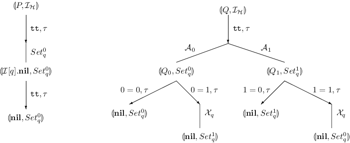
(Example 3.3 revisited) For the first example, we revisit the two ways of setting a quantum system to pure state |0⟩|0\rangle, presented in Example 3.3. According to the symbolic operational semantics presented in Fig. 3, the qLTSs rooted by ⦇P,ℐℋ⦈\llparenthesis P,\mathcal{I}_{\mathcal{H}}\rrparenthesis and ⦇Q,ℐℋ⦈\llparenthesis Q,\mathcal{I}_{\mathcal{H}}\rrparenthesis respectively can be depicted as in Fig. 4, where 𝒜i\mathcal{A}_{i} has the single Kraus operator |i⟩q​⟨i||i\rangle_{q}\langle i| for i=0,1i=0,1.

At the first glance, it is tempting to think that symbolic semantics provides no advantage in describing quantum processes, as the qLTSs in Fig. 4 are almost the same as the pLTSs in Fig. 2 (Indeed, the right-hand side qLTS in the former is even more complicated than the corresponding pLTS in the latter). However, pLTSs in Fig. 2 are depicted for a fixed quantum state ρ\rho; to characterise the behaviours of a quantum process, infinitely many such pLTSs must be given, although typically they share the same structure. On the other hand, the qLTSs in Fig. 4 specify a​l​lall possible behaviours of the processes, by means of the super-operators they can perform.
Refer to caption
Figure 4: qLTSs for two ways of setting a quantum system to |0⟩|0\rangle
Example 5.3.

This example shows the correctness of super-dense coding protocol. Let M=∑i=03i⁡|i~⟩​⟨i~|M=\sum_{i=0}^{3}i|\tilde{i}\rangle\langle\tilde{i}| be a 2-qubit measurement where i~\tilde{i} is the binary expansion of ii. Let 𝒞​𝒩\mathcal{CN} be the controlled-not operation and ℋ\mathcal{H} Hadamard operation. Then the quantum processes participating in super-dense coding protocol can be defined as follows:

A​l​i​c​e\displaystyle Alice =d​e​f\displaystyle\stackrel{{\scriptstyle def}}{{=}} 𝖼A?q1.∑0≤i≤3(ifx=ithenσi[q1].𝖾!q1.nil),\displaystyle{\sf{c}}_{A}?q_{1}.\sum_{0\leq i\leq 3}\left(\mbox{\bf{if}}\ x=i\ \mbox{\bf{then}}\ \sigma^{i}[q_{1}].{\sf{e}}!q_{1}.\mbox{\bf{nil}}\right),
B​o​b\displaystyle Bob =d​e​f\displaystyle\stackrel{{\scriptstyle def}}{{=}} 𝖼B​?​q2.𝖾​?​q1.𝒞​𝒩​[q1,q2].ℋ⁡[q1].M⁡[q1,q2;x].d!​x.nil,\displaystyle{\sf{c}}_{B}?q_{2}.{\sf{e}}?q_{1}.\mathcal{CN}[q_{1},q_{2}].\mathcal{H}[q_{1}].M[q_{1},q_{2};x].d!x.\mbox{\bf{nil}},
E​P​R\displaystyle EPR =d​e​f\displaystyle\stackrel{{\scriptstyle def}}{{=}} S​e​tΨ​[q1,q2].𝖼B!​q2.𝖼A!​q1.nil,\displaystyle Set^{\Psi}[q_{1},q_{2}].{\sf{c}}_{B}!q_{2}.{\sf{c}}_{A}!q_{1}.\mbox{\bf{nil}},
S​d​c\displaystyle Sdc =d​e​f\displaystyle\stackrel{{\scriptstyle def}}{{=}} c​?​x.(E​P​R​‖A​l​i​c​e‖​B​o​b)\{𝖼A,𝖼B,𝖾}.\displaystyle c?x.(EPR\|Alice\|Bob)\backslash\{{\sf{c}}_{A},{\sf{c}}_{B},{\sf{e}}\}.

The specification of super-dense coding protocol can be defined as:

S​d​cs​p​e​c=d​e​fc​?​x.τ7.S​e​tx​[q1,q2].d!​x.nilSdc_{spec}\stackrel{{\scriptstyle def}}{{=}}c?x.\tau^{7}.Set^{x}[q_{1},q_{2}].d!x.\mbox{\bf{nil}}

where

Setx[q1,q2].d!x.nil=∑i=03(ifx=ithenSeti[q1,q2].d!x.nil).Set^{x}[q_{1},q_{2}].d!x.\mbox{\bf{nil}}=\sum_{i=0}^{3}(\mbox{\bf{if}}\ x=i\ \mbox{\bf{then}}\ Set^{i}[q_{1},q_{2}].d!x.\mbox{\bf{nil}}).

Here S​e​tiSet^{i} and S​e​tΨSet^{\Psi} are the 2-qubit super-operators which set the target qubits to |i~⟩|\widetilde{i}\rangle and |Ψ⟩=(|00⟩+|11⟩)/2|\Psi\rangle=(|00\rangle+|11\rangle)/\sqrt{2}, respectively. We insert seven τ\tau’s in the specification to match the internal actions of S​d​cSdc. The qLTSs rooted from ⦇Sdcs​p​e​c,ℐℋ⦈\llparenthesis Sdc_{spec},\mathcal{I}_{\mathcal{H}}\rrparenthesis and ⦇Sdc,ℐℋ⦈\llparenthesis Sdc,\mathcal{I}_{\mathcal{H}}\rrparenthesis respectively are depicted in Fig. 5 where q~={q1,q2}\widetilde{q}=\{q_{1},q_{2}\}, 𝒜i~\mathcal{A}_{\widetilde{i}} is the super-operator with the single Kraus operator |i~⟩​⟨i~||\widetilde{i}\rangle\langle\widetilde{i}|, L={𝖼A,𝖼B,𝖾}L=\{{\sf{c}}_{A},{\sf{c}}_{B},{\sf{e}}\},

S​d​cx\displaystyle Sdc^{x} =\displaystyle= ((∑i=03(ifx=ithenσi[q1].𝖾!q1.nil))∥Bob)\{𝖾},\displaystyle\left(\left(\sum_{i=0}^{3}(\mbox{\bf{if}}\ x=i\ \mbox{\bf{then}}\ \sigma^{i}[q_{1}].{\sf{e}}!q_{1}.\mbox{\bf{nil}})\right)\|Bob\right)\backslash\{{\sf{e}}\},

and for simplicity, we only draw the transitions along the x=0x=0 branch.

Refer to captionRefer to caption\begin{array}[]{lr}\begin{array}[]{l}\includegraphics[width=195.12767pt]{sdc_spec.eps}\end{array}&\begin{array}[]{l}\includegraphics[width=195.12767pt]{sdc.eps}\end{array}\end{array}
Figure 5: qLTSs for ⦇Sdcs​p​e​c,ℐℋ⦈\llparenthesis Sdc_{spec},\mathcal{I}_{\mathcal{H}}\rrparenthesis and ⦇Sdc,ℐℋ⦈\llparenthesis Sdc,\mathcal{I}_{\mathcal{H}}\rrparenthesis

To conclude this subsection, we prove some useful properties of symbolic transitions.

Lemma 5.4.

If ⦇t,ℰ⦈⟶b,γΔ\llparenthesis t,\mathcal{E}\rrparenthesis\stackrel{{\scriptstyle b,\gamma}}{{\longrightarrow}}\Delta, then there exist super-operators {ℬi:i∈I}⊆C​P​(ℋ)\{\mathcal{B}_{i}:i\in I\}\subseteq CP(\mathcal{H}) and {ℱi:i∈I}⊆C​Pt​(ℋ)\{\mathcal{F}_{i}:i\in I\}\subseteq CP_{t}(\mathcal{H}), and process terms {ti:i∈I}⊆𝒯\{t_{i}:i\in I\}\subseteq\mathcal{T} such that

  1. (1)

    ∑i∈Iℬi≂ℐℋ\sum_{i\in I}\mathcal{B}_{i}\eqsim\mathcal{I}_{\mathcal{H}},

  2. (2)

    Δ=∑i∈Iℬi∙⦇ti,ℱiℰ⦈,\Delta=\sum_{i\in I}\mathcal{B}_{i}\bullet\llparenthesis t_{i},\mathcal{F}_{i}\mathcal{E}\rrparenthesis,

  3. (3)

    for any 𝒢∈C​Pt​(ℋ)\mathcal{G}\in CP_{t}(\mathcal{H}), ⦇t,𝒢⦈⟶b,γ∑i∈Iℬi∙⦇ti,ℱi𝒢⦈.\llparenthesis t,\mathcal{G}\rrparenthesis\stackrel{{\scriptstyle b,\gamma}}{{\longrightarrow}}\sum_{i\in I}\mathcal{B}_{i}\bullet\llparenthesis t_{i},\mathcal{F}_{i}\mathcal{G}\rrparenthesis.

Especially, if |I|>1|I|>1 then ℬi\mathcal{B}_{i} and ℱi\mathcal{F}_{i} take the forms as 𝒜r~ϕi\mathcal{A}^{\phi_{i}}_{\widetilde{r}} and S​e​tr~ϕiSet^{\phi_{i}}_{\widetilde{r}} in Eqs.(2) and (3), respectively.

Proof. Easy from the definition of inference rules. □\Box

The following lemmas show the relationship between transitions in ordinary semantics and in symbolic semantics. Let ψ{\psi} be an evaluation, α∈A​c​tc\alpha\in Act_{c}, and γ∈A​c​ts\gamma\in Act_{s}. We write α=ψγ\alpha=_{\psi}\gamma if either α=c!​v\alpha=c!v, γ=c!​e\gamma=c!e, and ψ⁡(e)=v{\psi}(e)=v, or γ=α\gamma=\alpha if neither of them is a classical output.

Lemma 5.5.

Suppose ⟨t​ψ,ρ⟩⟼αμ\langle t{\psi},\rho\rangle\stackrel{{\scriptstyle\alpha}}{{\longmapsto}}\mu. Then there exist b,Ib,I, ψ′{\psi}^{\prime}, {𝒜i:i∈I}⊆C​P​(ℋ)\{\mathcal{A}_{i}:i\in I\}\subseteq CP(\mathcal{H}), {ℰi:i∈I}⊆C​Pt​(ℋ)\{\mathcal{E}_{i}:i\in I\}\subseteq CP_{t}(\mathcal{H}), and {ti:i∈I}⊆𝒯\{t_{i}:i\in I\}\subseteq\mathcal{T}, such that ∑i∈I𝒜i≂ℐℋ\sum_{i\in I}\mathcal{A}_{i}\eqsim\mathcal{I}_{\mathcal{H}}, and

  1. (1)

    ψ⁡(b)=tt{\psi}(b)=\mbox{{tt}},

  2. (2)

    μ=∑i∈Itr⁡(𝒜i​(ρ))​⟨ti​ψ′,ℰi​(ρ)⟩\mu=\sum_{i\in I}{\rm tr}(\mathcal{A}_{i}(\rho))\langle t_{i}{\psi}^{\prime},\mathcal{E}_{i}(\rho)\rangle,

  3. (3)

    for any ℰ∈C​Pt​(ℋ)\mathcal{E}\in CP_{t}(\mathcal{H}), ⦇t,ℰ⦈⟶b,γ∑i∈I𝒜i∙⦇ti,ℰiℰ⦈\llparenthesis t,\mathcal{E}\rrparenthesis\stackrel{{\scriptstyle b,\gamma}}{{\longrightarrow}}\sum_{i\in I}\mathcal{A}_{i}\bullet\llparenthesis t_{i},\mathcal{E}_{i}\mathcal{E}\rrparenthesis, where

    1. (a)

      if α=c​?​v\alpha=c?v then γ=c​?​x\gamma=c?x for some x∉f​v​(t)x\not\in fv(t), and ψ′=ψ​{v/x}{\psi}^{\prime}={\psi}\{v/x\},

    2. (b)

      otherwise, γ=ψα\gamma=_{\psi}\alpha and ψ′=ψ{\psi}^{\prime}={\psi}.

Proof. We prove by induction on the depth of the inference by which the action ⟨t​ψ,ρ⟩⟼αμ\langle t{\psi},\rho\rangle\stackrel{{\scriptstyle\alpha}}{{\longmapsto}}\mu is inferred. We argue by cases on the form of tt.

  1. (1)

    t=c​?​x.t′t=c?x.t^{\prime}. Then t​ψ=c​?​x.ut{\psi}=c?x.u where uu is the process term obtained from t′t^{\prime} by instantiating all the free variables in f​v​(t′)−{x}fv(t^{\prime})-\{x\} according to ψ{\psi}. By Rule C​-​I​n​pcC\textrm{-}Inp_{c} we deduce that α=c​?​v\alpha=c?v for some v∈𝖱𝖾𝖺𝗅v\in{\sf{Real}} and μ=⟨P,ρ⟩\mu=\langle P,\rho\rangle where P=u⁡{v/x}=t′​ψ​{v/x}P=u\{v/x\}=t^{\prime}{\psi}\{v/x\}. By Rule A​c​tsAct_{s}, for any ℰ∈C​Pt​(ℋ)\mathcal{E}\in CP_{t}(\mathcal{H}), we have ⦇t,ℰ⦈⟶tt,c​?​x⦇t′,ℰ⦈\llparenthesis t,\mathcal{E}\rrparenthesis\stackrel{{\scriptstyle\mbox{{tt}},c?x}}{{\longrightarrow}}\llparenthesis t^{\prime},\mathcal{E}\rrparenthesis. So we need only to take b=ttb=\mbox{{tt}}, |I|=1|I|=1, ti=t′t_{i}=t^{\prime}, 𝒜i=ℰi=ℐℋ\mathcal{A}_{i}=\mathcal{E}_{i}=\mathcal{I}_{\mathcal{H}}.

  2. (2)

    t=c!​e.t′t=c!e.t^{\prime}. Then t​ψ=c!​ψ​(e).(t′​ψ)t{\psi}=c!{\psi}(e).(t^{\prime}{\psi}), and by Rule C​-​O​u​tcC\textrm{-}Out_{c} we deduce that α=c!​ψ​(e)\alpha=c!{\psi}(e) and μ=⟨t′​ψ,ρ⟩\mu=\langle t^{\prime}{\psi},\rho\rangle. By Rule A​c​tsAct_{s}, for any ℰ∈C​Pt​(ℋ)\mathcal{E}\in CP_{t}(\mathcal{H}), we have ⦇t,ℰ⦈⟶tt,c!​e⦇t′,ℰ⦈\llparenthesis t,\mathcal{E}\rrparenthesis\stackrel{{\scriptstyle\mbox{{tt}},c!e}}{{\longrightarrow}}\llparenthesis t^{\prime},\mathcal{E}\rrparenthesis. So we need only to take b=ttb=\mbox{{tt}}, |I|=1|I|=1, ti=t′t_{i}=t^{\prime}, 𝒜i=ℰi=ℐℋ\mathcal{A}_{i}=\mathcal{E}_{i}=\mathcal{I}_{\mathcal{H}} as well.

  3. (3)

    t=𝖼​?​q.t′t={\sf{c}}?q.t^{\prime}. Then t​ψ=𝖼​?​q.(t′​ψ)t{\psi}={\sf{c}}?q.(t^{\prime}{\psi}), and by Rule Q​-​I​n​pcQ\textrm{-}Inp_{c} we deduce that α=𝖼​?​r\alpha={\sf{c}}?r for some r∉q​v​(t)r\not\in qv(t) and μ=⟨(t′​ψ)​{r/q},ρ⟩\mu=\langle(t^{\prime}{\psi})\{r/q\},\rho\rangle. By Rule A​c​tsAct_{s} and α\alpha-conversion, for any ℰ∈C​Pt​(ℋ)\mathcal{E}\in CP_{t}(\mathcal{H}), we have ⦇t,ℰ⦈⟶tt,𝖼​?​r⦇t′{r/q},ℰ⦈\llparenthesis t,\mathcal{E}\rrparenthesis\stackrel{{\scriptstyle\mbox{{tt}},{\sf{c}}?r}}{{\longrightarrow}}\llparenthesis t^{\prime}\{r/q\},\mathcal{E}\rrparenthesis. So we need only to take b=ttb=\mbox{{tt}}, |I|=1|I|=1, ti=t′​{r/q}t_{i}=t^{\prime}\{r/q\}, 𝒜i=ℰi=ℐℋ\mathcal{A}_{i}=\mathcal{E}_{i}=\mathcal{I}_{\mathcal{H}}.

  4. (4)

    t=M⁡[q~;x].t′t=M[\widetilde{q};x].t^{\prime}. Then t​ψ=M⁡[q~;x].ut{\psi}=M[\widetilde{q};x].u where uu is the process term obtained from t′t^{\prime} by instantiating all the free variables in f​v​(t′)−{x}fv(t^{\prime})-\{x\} according to ψ{\psi}. Let M=∑i∈Iλi​|ϕi⟩​⟨ϕi|M=\sum_{i\in I}\lambda_{i}|\phi_{i}\rangle\langle\phi_{i}|. By Rule M​e​a​scMeas_{c} we deduce that α=τ\alpha=\tau and μ=∑i∈Itr⁡(𝒜i​(ρ))​⟨Pi,ℰi​(ρ)⟩\mu=\sum_{i\in I}{\rm tr}(\mathcal{A}_{i}(\rho))\langle P_{i},\mathcal{E}_{i}(\rho)\rangle where Pi=u⁡{λi/x}=t′​{λi/x}​ψP_{i}=u\{\lambda_{i}/x\}=t^{\prime}\{\lambda_{i}/x\}{\psi}, 𝒜i={|ϕi⟩​⟨ϕi|}\mathcal{A}_{i}=\{|\phi_{i}\rangle\langle\phi_{i}|\}, and ℰi={|ϕi⟩​⟨ϕj|:j∈I}\mathcal{E}_{i}=\{|\phi_{i}\rangle\langle\phi_{j}|:j\in I\}. Take b=ttb=\mbox{{tt}}. By Rule M​e​a​ssMeas_{s}, for any ℰ∈C​Pt​(ℋ)\mathcal{E}\in CP_{t}(\mathcal{H}), we have ⦇t,ℰ⦈⟶b,τ∑i∈I𝒜i∙⦇t′{λi/x},ℰiℰ⦈\llparenthesis t,\mathcal{E}\rrparenthesis\stackrel{{\scriptstyle b,\tau}}{{\longrightarrow}}\sum_{i\in I}\mathcal{A}_{i}\bullet\llparenthesis t^{\prime}\{\lambda_{i}/x\},\mathcal{E}_{i}\mathcal{E}\rrparenthesis.

  5. (5)

    t=t1|t2t=t_{1}\|t_{2}. Then t​ψ=t1​ψ|t2​ψt{\psi}=t_{1}{\psi}\|t_{2}{\psi}. There are two sub-cases to consider:

    1. (a)

      The action is caused by one of the components, say ⟨t1​ψ,ρ⟩⟼αμ1\langle t_{1}{\psi},\rho\rangle\stackrel{{\scriptstyle\alpha}}{{\longmapsto}}\mu_{1}. Then we have q​b​v​(α)∩q​v​(t2​ψ)=∅qbv(\alpha)\cap qv(t_{2}{\psi})=\emptyset, and μ=μ1|t2​ψ\mu=\mu_{1}\|t_{2}{\psi}. By induction, there exist b,Ib,I, tit_{i}, 𝒜i,ℰi\mathcal{A}_{i},\mathcal{E}_{i}, i∈Ii\in I, such that ψ⁡(b)=tt{\psi}(b)=\mbox{{tt}}, μ1=∑i∈Itr⁡(𝒜i​(ρ))​⟨ti​ψ′,ℰi​(ρ)⟩\mu_{1}=\sum_{i\in I}{\rm tr}(\mathcal{A}_{i}(\rho))\langle t_{i}{\psi}^{\prime},\mathcal{E}_{i}(\rho)\rangle, and for any ℰ∈C​Pt​(ℋ)\mathcal{E}\in CP_{t}(\mathcal{H}), ⦇t1,ℰ⦈⟶b,γ∑i∈I𝒜i∙⦇ti,ℰiℰ⦈\llparenthesis t_{1},\mathcal{E}\rrparenthesis\stackrel{{\scriptstyle b,\gamma}}{{\longrightarrow}}\sum_{i\in I}\mathcal{A}_{i}\bullet\llparenthesis t_{i},\mathcal{E}_{i}\mathcal{E}\rrparenthesis. Note that by α\alpha-conversion, when γ=c​?​x\gamma=c?x, we can always take xx such that x∉f​v​(t2)x\not\in fv(t_{2}), and consequently, (ti∥t2)ψ′=tiψ′∥t2ψ(t_{i}\|t_{2}){\psi}^{\prime}=t_{i}{\psi}^{\prime}\|t_{2}{\psi}. Finally, we have ⦇t,ℰ⦈⟶b,γ∑i∈I𝒜i∙⦇ti∥t2,ℰiℰ⦈\llparenthesis t,\mathcal{E}\rrparenthesis\stackrel{{\scriptstyle b,\gamma}}{{\longrightarrow}}\sum_{i\in I}\mathcal{A}_{i}\bullet\llparenthesis t_{i}\|t_{2},\mathcal{E}_{i}\mathcal{E}\rrparenthesis, using Rule P​a​rsPar_{s}.

    2. (b)

      The action is caused by a (classical or quantum) communication. Here we only detail the case when ⟨t1​ψ,ρ⟩⟼c​?​v⟨P1,ρ⟩\langle t_{1}{\psi},\rho\rangle\stackrel{{\scriptstyle c?v}}{{\longmapsto}}\langle P_{1},\rho\rangle, ⟨t2​ψ,ρ⟩⟼c!​v⟨P2,ρ⟩\langle t_{2}{\psi},\rho\rangle\stackrel{{\scriptstyle c!v}}{{\longmapsto}}\langle P_{2},\rho\rangle, α=τ\alpha=\tau, and μ=⟨P1∥P2,ρ⟩\mu=\langle P_{1}\|P_{2},\rho\rangle. Then by induction, there exist b1b_{1}, b2b_{2}, t1′t^{\prime}_{1}, t2′t^{\prime}_{2} such that ψ⁡(b1∧b2)=tt{\psi}(b_{1}\wedge b_{2})=\mbox{{tt}}, P1=t1′​ψ′P_{1}=t_{1}^{\prime}{\psi}^{\prime}, P2=t2′​ψP_{2}=t_{2}^{\prime}{\psi}, and for any ℰ∈C​Pt​(ℋ)\mathcal{E}\in CP_{t}(\mathcal{H}), ⦇t1,ℰ⦈⟶b1,c​?​x⦇t1′,ℰ⦈\llparenthesis t_{1},\mathcal{E}\rrparenthesis\stackrel{{\scriptstyle b_{1},c?x}}{{\longrightarrow}}\llparenthesis t_{1}^{\prime},\mathcal{E}\rrparenthesis and ⦇t2,ℰ⦈⟶b2,c!​e⦇t2′,ℰ⦈\llparenthesis t_{2},\mathcal{E}\rrparenthesis\stackrel{{\scriptstyle b_{2},c!e}}{{\longrightarrow}}\llparenthesis t_{2}^{\prime},\mathcal{E}\rrparenthesis, where x∉f​v​(t1)x\not\in fv(t_{1}), ψ′=ψ​{v/x}{\psi}^{\prime}={\psi}\{v/x\}, and ψ⁡(e)=v{\psi}(e)=v. Thus

      (t1′{e/x}∥t2′)ψ=t1′{e/x}ψ∥t2′ψ=t1′ψ{v/x}∥t2′ψ=t1′ψ′∥t2′ψ=P1∥P2.\displaystyle(t_{1}^{\prime}\{e/x\}\|t_{2}^{\prime}){\psi}=t_{1}^{\prime}\{e/x\}{\psi}\|t_{2}^{\prime}{\psi}=t_{1}^{\prime}{\psi}\{v/x\}\|t_{2}^{\prime}{\psi}=t_{1}^{\prime}{\psi}^{\prime}\|t_{2}^{\prime}{\psi}=P_{1}\|P_{2}.

      Finally, we have ⦇t,ℰ⦈⟶b1∧b2,τ⦇t1′{e/x}∥t2′,ℰ⦈\llparenthesis t,\mathcal{E}\rrparenthesis\stackrel{{\scriptstyle b_{1}\wedge b_{2},\tau}}{{\longrightarrow}}\llparenthesis t_{1}^{\prime}\{e/x\}\|t_{2}^{\prime},\mathcal{E}\rrparenthesis, using Rule Q​-​C​o​msQ\textrm{-}Com_{s}.

  6. (6)

    Other cases. Similar to the cases we discussed above. □\Box

Lemma 5.6.

Suppose ⦇t,ℰ⦈⟶b,γΔ\llparenthesis t,\mathcal{E}\rrparenthesis\stackrel{{\scriptstyle b,\gamma}}{{\longrightarrow}}\Delta. Then there exist II, {𝒜i:i∈I}⊆C​P​(ℋ)\{\mathcal{A}_{i}:i\in I\}\subseteq CP(\mathcal{H}), {ℰi:i∈I}⊆C​Pt​(ℋ)\{\mathcal{E}_{i}:i\in I\}\subseteq CP_{t}(\mathcal{H}), and {ti:i∈I}⊆𝒯\{t_{i}:i\in I\}\subseteq\mathcal{T}, such that ∑i∈I𝒜i≂ℐℋ\sum_{i\in I}\mathcal{A}_{i}\eqsim\mathcal{I}_{\mathcal{H}}, and

  1. (1)

    Δ=∑i∈I𝒜i∙⦇ti,ℰiℰ⦈\Delta=\sum_{i\in I}\mathcal{A}_{i}\bullet\llparenthesis t_{i},\mathcal{E}_{i}\mathcal{E}\rrparenthesis,

  2. (2)

    for any ψ{\psi} and ρ\rho, ψ⁡(b)=tt{\psi}(b)=\mbox{{tt}} implies ⟨t​ψ,ρ⟩⟼α∑i∈Itr⁡(𝒜i​(ρ))​⟨ti​ψ′,ℰi​(ρ)⟩\langle t{\psi},\rho\rangle\stackrel{{\scriptstyle\alpha}}{{\longmapsto}}\sum_{i\in I}{\rm tr}(\mathcal{A}_{i}(\rho))\langle t_{i}{\psi}^{\prime},\mathcal{E}_{i}(\rho)\rangle where

    1. (a)

      if γ=c​?​x\gamma=c?x then α=c​?​v\alpha=c?v for some v∈𝖱𝖾𝖺𝗅v\in{\sf{Real}}, and ψ′=ψ​{v/x}{\psi}^{\prime}={\psi}\{v/x\},

    2. (b)

      otherwise, γ=ψα\gamma=_{\psi}\alpha and ψ′=ψ{\psi}^{\prime}={\psi}.

Proof. Similar to Lemma 5.5. □\Box

5.3 Symbolic bisimulation

Let 𝒮⊆S​N×S​N\mathcal{S}\subseteq SN\times SN be an equivalence relation. We lift 𝒮\mathcal{S} to 𝒟​i​s​tℋ​(S​N)×𝒟​i​s​tℋ​(S​N)\mathcal{D}ist_{\mathcal{H}}(SN)\times\mathcal{D}ist_{\mathcal{H}}(SN) by defining Δ​𝒮​Ξ\Delta\mathcal{S}\Xi if for any equivalence class T∈S​N/𝒮T\in SN/\mathcal{S}, Δ⁡(T)≂Ξ⁡(T)\Delta(T)\eqsim\Xi(T); that is, ∑⦇t,ℰ⦈∈TΔ(⦇t,ℰ⦈)≂∑⦇t,ℰ⦈∈TΞ(⦇t,ℰ⦈)\sum_{\llparenthesis t,\mathcal{E}\rrparenthesis\in T}\Delta(\llparenthesis t,\mathcal{E}\rrparenthesis)\eqsim\sum_{\llparenthesis t,\mathcal{E}\rrparenthesis\in T}\Xi(\llparenthesis t,\mathcal{E}\rrparenthesis). We write γ=bγ′\gamma=_{b}\gamma^{\prime} if either γ=c!​e\gamma=c!e, γ′=c!​e′\gamma^{\prime}=c!e^{\prime}, and b→e=e′b\rightarrow e=e^{\prime}, or γ=γ′\gamma=\gamma^{\prime} if neither of them is a classical output.

Definition 5.7.

Let 𝔖={𝒮b:b∈B​E​x​p}\mathfrak{S}=\{\mathcal{S}^{b}:b\in BExp\} be a family of equivalence relations on S​NSN. 𝔖\mathfrak{S} is called a symbolic (open) bisimulation if for any b∈B​E​x​pb\in BExp, ⦇t,ℰ⦈𝒮b⦇u,ℱ⦈\llparenthesis t,\mathcal{E}\rrparenthesis\mathcal{S}^{b}\llparenthesis u,\mathcal{F}\rrparenthesis implies that

  1. (1)

    q​v​(t)=q​v​(u)qv(t)=qv(u) and ℰ≂q​v​(t)¯ℱ\mathcal{E}\eqsim_{\overline{qv(t)}}\mathcal{F}, if bb is satisfiable;

  2. (2)

    for any 𝒢∈C​Pt​(ℋq​v​(t)¯)\mathcal{G}\in CP_{t}(\mathcal{H}_{\overline{qv(t)}}), whenever ⦇t,𝒢ℰ⦈⟶b1,γΔ\llparenthesis t,\mathcal{G}\mathcal{E}\rrparenthesis\stackrel{{\scriptstyle b_{1},\gamma}}{{\longrightarrow}}\Delta with b​v​(γ)∩f​v​(b,t,u)=∅bv(\gamma)\cap fv(b,t,u)=\emptyset, then there exists a collection of booleans BB such that b∧b1→⋁Bb\wedge b_{1}\rightarrow\bigvee B and ∀b′∈B\forall\ b^{\prime}\in B, ∃b2,γ′\exists b_{2},\gamma^{\prime} with b′→b2b^{\prime}\rightarrow b_{2}, γ=b′γ′\gamma=_{b^{\prime}}\gamma^{\prime}, ⦇u,𝒢ℱ⦈⟶b2,γ′Ξ\llparenthesis u,\mathcal{G}\mathcal{F}\rrparenthesis\stackrel{{\scriptstyle b_{2},{\gamma^{\prime}}}}{{\longrightarrow}}\Xi, and (𝒢​ℰ∙Δ)​𝒮b′​(𝒢​ℱ∙Ξ)(\mathcal{G}\mathcal{E}\bullet\Delta)\mathcal{S}^{b^{\prime}}(\mathcal{G}\mathcal{F}\bullet\Xi).

Two configurations ⦇t,ℰ⦈\llparenthesis t,\mathcal{E}\rrparenthesis and ⦇u,ℱ⦈\llparenthesis u,\mathcal{F}\rrparenthesis are symbolically bb-bisimilar, denoted by ⦇t,ℰ⦈∼b⦇u,ℱ⦈\llparenthesis t,\mathcal{E}\rrparenthesis\sim^{b}\llparenthesis u,\mathcal{F}\rrparenthesis, if there exists a symbolic bisimulation 𝔖={𝒮b:b∈B​E​x​p}\mathfrak{S}=\{\mathcal{S}^{b}:b\in BExp\} such that ⦇t,ℰ⦈𝒮b⦇u,ℱ⦈\llparenthesis t,\mathcal{E}\rrparenthesis\mathcal{S}^{b}\llparenthesis u,\mathcal{F}\rrparenthesis. Two quantum process terms tt and uu are symbolically bb-bisimilar, denoted by t∼but\sim^{b}u, if ⦇t,ℐℋ⦈∼b⦇u,ℐℋ⦈\llparenthesis t,\mathcal{I}_{\mathcal{H}}\rrparenthesis\sim^{b}\llparenthesis u,\mathcal{I}_{\mathcal{H}}\rrparenthesis. When b=ttb=\mbox{{tt}}, we simply write t∼ut\sim u.

To show the usage of symbolic bisimulation, we revisit the examples presented in Section 5.2 to show that the proposed protocols indeed achieve the desired goals. Let A~={Ai:i∈I}\widetilde{A}=\{A_{i}:i\in I\} be a set of disjoint subsets of snapshots. An equivalence relation 𝒮\mathcal{S} is said to be generated by A~\widetilde{A} if its equivalence classes on the set of snapshots ∪i∈IAi\cup_{i\in I}A_{i} are given by the partition A~\widetilde{A}, and it is the identity relation on SN−∪i∈IAiSN-\cup_{i\in I}A_{i}.

Example 5.8.

(Example 5.2 revisited) This example is devoted to showing rigorously that the two ways of setting a quantum system to the pure state |0⟩|0\rangle, presented in Examples 3.3 and 5.2, are indeed bisimilar. Let

A\displaystyle A =\displaystyle= {⦇P,ℐℋ⦈,⦇Q,ℐℋ⦈},\displaystyle\{\llparenthesis P,\mathcal{I}_{\mathcal{H}}\rrparenthesis,\llparenthesis Q,\mathcal{I}_{\mathcal{H}}\rrparenthesis\},
B\displaystyle B =\displaystyle= {⦇ℐ[q].nil,Setq0⦈,⦇Q0,Setq0⦈,⦇Q1,Setq1⦈}\displaystyle\{\llparenthesis\mathcal{I}[q].\mbox{\bf{nil}},Set^{0}_{q}\rrparenthesis,\llparenthesis Q_{0},Set^{0}_{q}\rrparenthesis,\llparenthesis Q_{1},Set^{1}_{q}\rrparenthesis\}

and 𝒮′\mathcal{S}^{\prime} be the equivalence relation generated by {A,B}\{A,B\}. It is easy to check that the family {𝒮b:b∈B​E​x​p}\{\mathcal{S}^{b}:b\in BExp\}, where 𝒮b=𝒮′\mathcal{S}^{b}=\mathcal{S}^{\prime} for any b∈B​E​x​pb\in BExp, is a symbolic bisimulation. Thus P∼QP\sim Q.

Example 5.9.

(Superdense coding revisited) This example is devoted to proving rigorously that the protocol presented in Example 5.3 indeed sends two bits of classical information from Alice to Bob by transmitting a qubit. For that purpose, we need to show that ⦇Sdcs​p​e​c,ℐℋ⦈∼tt⦇Sdc,ℐℋ⦈\llparenthesis Sdc_{spec},\mathcal{I}_{\mathcal{H}}\rrparenthesis\sim^{\mbox{{tt}}}\llparenthesis Sdc,\mathcal{I}_{\mathcal{H}}\rrparenthesis. Indeed, let

A\displaystyle A =\displaystyle= {⦇Sdcs​p​e​c,ℐℋ⦈,⦇Sdc,ℐℋ⦈},\displaystyle\{\llparenthesis Sdc_{spec},\mathcal{I}_{\mathcal{H}}\rrparenthesis,\llparenthesis Sdc,\mathcal{I}_{\mathcal{H}}\rrparenthesis\},
Bj\displaystyle B^{j} =\displaystyle= {⦇t,ℰ⦈:d(⦇t,ℰ⦈)=j},\displaystyle\{\llparenthesis t,\mathcal{E}\rrparenthesis:d(\llparenthesis t,\mathcal{E}\rrparenthesis)=j\},
Cik\displaystyle C^{k}_{i} =\displaystyle= {⦇t,ℰ⦈:⦇t,ℰ⦈ along the branch of x=i, and d(⦇t,ℰ⦈)=k},\displaystyle\{\llparenthesis t,\mathcal{E}\rrparenthesis:\llparenthesis t,\mathcal{E}\rrparenthesis\mbox{ along the branch of $x=i$, and }d(\llparenthesis t,\mathcal{E}\rrparenthesis)=k\},

where d(⦇t,ℰ⦈)d(\llparenthesis t,\mathcal{E}\rrparenthesis) is the depth of the node ⦇t,ℰ⦈\llparenthesis t,\mathcal{E}\rrparenthesis from the root of its corresponding qLTS, 0<j≤40<j\leq 4, 0≤i≤30\leq i\leq 3, and 5≤k≤105\leq k\leq 10. Let 𝒮1tt\mathcal{S}_{1}^{\mbox{{tt}}} be the equivalence relation generated by {A,B1,B2,B3,B4}\{A,B^{1},B^{2},B^{3},B^{4}\}, and 𝒮1x=i\mathcal{S}_{1}^{x=i} generated by {Cik:5≤k≤10}\{C^{k}_{i}:5\leq k\leq 10\}. For any b∈B​E​x​pb\in BExp, let 𝒮b\mathcal{S}^{b} be 𝒮1x=i\mathcal{S}_{1}^{x=i} if b↔x=ib\leftrightarrow x=i, 𝒮1tt\mathcal{S}_{1}^{\mbox{{tt}}} if b↔ttb\leftrightarrow\mbox{{tt}}, and 𝖨𝖽S​N{\sf{Id}}_{SN} otherwise. Then it is easy to check that 𝔖={𝒮b:b∈B​E​x​p}\mathfrak{S}=\{\mathcal{S}^{b}:b\in BExp\} is a symbolic bisimulation.

In the following, we denote by 𝒮∗\mathcal{S}^{*} the equivalence closure of a relation 𝒮\mathcal{S}.

Definition 5.10.

A relation family 𝔖={𝒮b:b∈B​E​x​p}\mathfrak{S}=\{\mathcal{S}^{b}:b\in BExp\} is called decreasing, if for any b,b′∈B​E​x​pb,b^{\prime}\in BExp with b→b′b\rightarrow b^{\prime}, we have 𝒮b′⊆𝒮b\mathcal{S}^{b^{\prime}}\subseteq\mathcal{S}^{b}.

Lemma 5.11.

Let 𝔖={𝒮b:b∈B​E​x​p}\mathfrak{S}=\{\mathcal{S}^{b}:b\in BExp\} be a symbolic bisimulation. Then there exists a decreasing symbolic bisimulation 𝔘={𝒰b:b∈B​E​x​p}\mathfrak{U}=\{\mathcal{U}^{b}:b\in BExp\} such that for each b∈B​E​x​pb\in BExp, 𝒮b⊆𝒰b\mathcal{S}^{b}\subseteq\mathcal{U}^{b}.

Proof. Suppose 𝔖={𝒮b:b∈B​E​x​p}\mathfrak{S}=\{\mathcal{S}^{b}:b\in BExp\} is a symbolic bisimulation. For each b∈B​E​x​pb\in BExp, let

𝒰1b=⋃{𝒮b′:b→b′}​ and ​𝒰b=(𝒰1b)∗.\mathcal{U}_{1}^{b}=\bigcup\{\mathcal{S}^{b^{\prime}}:b\rightarrow b^{\prime}\}\mbox{ and }\mathcal{U}^{b}=(\mathcal{U}_{1}^{b})^{*}.

Obviously, 𝔘={𝒰b:b∈B​E​x​p}\mathfrak{U}=\{\mathcal{U}^{b}:b\in BExp\} is decreasing. We have to show that 𝔘\mathfrak{U} is a symbolic bisimulation.

Let b∈B​E​x​pb\in BExp and ⦇t,ℰ⦈𝒰b⦇u,ℱ⦈\llparenthesis t,\mathcal{E}\rrparenthesis\mathcal{U}^{b}\llparenthesis u,\mathcal{F}\rrparenthesis. Note that 𝒰1b\mathcal{U}_{1}^{b} is both reflexive and symmetric. So 𝒰b\mathcal{U}^{b} is actually the transitive closure of 𝒰1b\mathcal{U}_{1}^{b}, and there exist n≥1n\geq 1 and a sequence of snapshots ⦇ti,ℰi⦈\llparenthesis t_{i},\mathcal{E}_{i}\rrparenthesis, 0≤i≤n0\leq i\leq n, such that ⦇t,ℰ⦈=⦇t0,ℰ0⦈\llparenthesis t,\mathcal{E}\rrparenthesis=\llparenthesis t_{0},\mathcal{E}_{0}\rrparenthesis, ⦇u,ℱ⦈=⦇tn,ℰn⦈\llparenthesis u,\mathcal{F}\rrparenthesis=\llparenthesis t_{n},\mathcal{E}_{n}\rrparenthesis, and for each 0≤i≤n−10\leq i\leq n-1, ⦇ti,ℰi⦈𝒰1b⦇ti+1,ℰi+1⦈\llparenthesis t_{i},\mathcal{E}_{i}\rrparenthesis\mathcal{U}_{1}^{b}\llparenthesis t_{i+1},\mathcal{E}_{i+1}\rrparenthesis. For the sake of simplicity, we assume n=2n=2. That is, there exists ⦇s,𝒢⦈\llparenthesis s,\mathcal{G}\rrparenthesis such that ⦇t,ℰ⦈𝒮b1⦇s,𝒢⦈𝒮b2⦇u,ℱ⦈\llparenthesis t,\mathcal{E}\rrparenthesis\mathcal{S}^{b_{1}}\llparenthesis s,\mathcal{G}\rrparenthesis\mathcal{S}^{b_{2}}\llparenthesis u,\mathcal{F}\rrparenthesis with b→b1∧b2b\rightarrow b_{1}\wedge b_{2}. The general case is more tedious but similar.

First we check that if bb is satisfiable, then q​v​(t)=q​v​(s)=q​v​(u)qv(t)=qv(s)=qv(u) and ℰ≂q​v​(t)¯𝒢≂q​v​(t)¯ℱ\mathcal{E}\eqsim_{\overline{qv(t)}}\mathcal{G}\eqsim_{\overline{qv(t)}}\mathcal{F}. Now for any 𝒢′∈C​Pt​(ℋq​v​(t)¯)\mathcal{G}^{\prime}\in CP_{t}(\mathcal{H}_{\overline{qv(t)}}), suppose ⦇t,𝒢′ℰ⦈⟶b1′,γΔ\llparenthesis t,\mathcal{G}^{\prime}\mathcal{E}\rrparenthesis\stackrel{{\scriptstyle b^{\prime}_{1},\gamma}}{{\longrightarrow}}\Delta with b​v​(γ)∩f​v​(b1,t,u)=∅bv(\gamma)\cap fv(b_{1},t,u)=\emptyset. By α\alpha-conversion, we may assume further that b​v​(γ)∩f​v​(s)=∅bv(\gamma)\cap fv(s)=\emptyset. From ⦇t,ℰ⦈𝒮b1⦇s,𝒢⦈\llparenthesis t,\mathcal{E}\rrparenthesis\mathcal{S}^{b_{1}}\llparenthesis s,\mathcal{G}\rrparenthesis, there exists a collection of booleans {ci:1≤i≤n}\{c_{i}:1\leq i\leq n\} such that b1∧b1′→⋁cib_{1}\wedge b_{1}^{\prime}\rightarrow\bigvee c_{i} and for any ii, ∃ci′,γi\exists c_{i}^{\prime},\gamma_{i} with ci→ci′c_{i}\rightarrow c_{i}^{\prime}, γ=ciγi\gamma=_{c_{i}}\gamma_{i}, ⦇s,𝒢′𝒢⦈⟶ci′,γiΘ\llparenthesis s,\mathcal{G}^{\prime}\mathcal{G}\rrparenthesis\stackrel{{\scriptstyle c_{i}^{\prime},{\gamma_{i}}}}{{\longrightarrow}}\Theta, and (𝒢′​ℰ∙Δ)​𝒮ci​(𝒢′​𝒢∙Θ)(\mathcal{G}^{\prime}\mathcal{E}\bullet\Delta)\mathcal{S}^{c_{i}}(\mathcal{G}^{\prime}\mathcal{G}\bullet\Theta). By α\alpha-conversion, we can again assume that for each ii, b​v​(γi)∩f​v​(b2,s,u)=∅bv(\gamma_{i})\cap fv(b_{2},s,u)=\emptyset. Now by the assumption that ⦇s,𝒢⦈𝒮b2⦇u,ℱ⦈\llparenthesis s,\mathcal{G}\rrparenthesis\mathcal{S}^{b_{2}}\llparenthesis u,\mathcal{F}\rrparenthesis, there exists a collection of booleans {di​j:1≤j≤ni}\{d_{ij}:1\leq j\leq n_{i}\} such that b2∧ci′→⋁jdi​jb_{2}\wedge c_{i}^{\prime}\rightarrow\bigvee_{j}d_{ij} and for any di​jd_{ij}, ∃di​j′,γi​j\exists d^{\prime}_{ij},\gamma_{ij} with di​j→di​j′d_{ij}\rightarrow d^{\prime}_{ij}, γi​j=di​jγi\gamma_{ij}=_{d_{ij}}\gamma_{i}, ⦇u,𝒢′ℱ⦈⟶di​j′,γi​jΞ\llparenthesis u,\mathcal{G}^{\prime}\mathcal{F}\rrparenthesis\stackrel{{\scriptstyle d^{\prime}_{ij},{\gamma_{ij}}}}{{\longrightarrow}}\Xi, and (𝒢′​𝒢∙Θ)​𝒮di​j​(𝒢′​ℱ∙Ξ)(\mathcal{G}^{\prime}\mathcal{G}\bullet\Theta)\mathcal{S}^{d_{ij}}(\mathcal{G}^{\prime}\mathcal{F}\bullet\Xi).

Now let

B={b∧ci∧di​j:1≤i≤n,1≤j≤ni}.B=\{b\wedge c_{i}\wedge d_{ij}:1\leq i\leq n,1\leq j\leq n_{i}\}.

From the fact that b→b1∧b2b\rightarrow b_{1}\wedge b_{2}, it is easy to check that b∧b1′→⋁Bb\wedge b^{\prime}_{1}\rightarrow\bigvee B. For any c=b∧ci∧di​jc=b\wedge c_{i}\wedge d_{ij}, we take c′=di​j′c^{\prime}=d^{\prime}_{ij} and γ′=γi​j\gamma^{\prime}=\gamma_{ij}. Then c→c′c\rightarrow c^{\prime}, γ′=cγ\gamma^{\prime}=_{c}\gamma, and ⦇u,𝒢′ℱ⦈⟶c′,γ′Ξ\llparenthesis u,\mathcal{G}^{\prime}\mathcal{F}\rrparenthesis\stackrel{{\scriptstyle c^{\prime},{\gamma^{\prime}}}}{{\longrightarrow}}\Xi. Furthermore, by the fact that c→cic\rightarrow c_{i} and the definition of 𝒰c\mathcal{U}^{c}, we have (𝒢′​ℰ∙Δ)​𝒰c​(𝒢′​𝒢∙Θ)(\mathcal{G}^{\prime}\mathcal{E}\bullet\Delta)\mathcal{U}^{c}(\mathcal{G}^{\prime}\mathcal{G}\bullet\Theta) indeed. Similarly, (𝒢′​𝒢∙Θ)​𝒰c​(𝒢′​ℱ∙Ξ)(\mathcal{G}^{\prime}\mathcal{G}\bullet\Theta)\mathcal{U}^{c}(\mathcal{G}^{\prime}\mathcal{F}\bullet\Xi). Thus (𝒢′​ℰ∙Δ)​𝒰c​(𝒢′​ℱ∙Ξ)(\mathcal{G}^{\prime}\mathcal{E}\bullet\Delta)\mathcal{U}^{c}(\mathcal{G}^{\prime}\mathcal{F}\bullet\Xi) as required. □\Box

Lemma 5.12.

Let decreasing families 𝔖i={𝒮ib:b∈B​E​x​p}\mathfrak{S}_{i}=\{\mathcal{S}_{i}^{b}:b\in BExp\}, i=1,2i=1,2, be symbolic bisimulations. Then the family 𝔖={(𝒮1b​𝒮2b)∗:b∈B​E​x​p}\mathfrak{S}=\{(\mathcal{S}_{1}^{b}\mathcal{S}_{2}^{b})^{*}:b\in BExp\} is also a symbolic bisimulation.

Proof. Let b∈B​E​x​pb\in BExp and ⦇t,ℰ⦈(𝒮1b𝒮2b)∗⦇u,ℱ⦈\llparenthesis t,\mathcal{E}\rrparenthesis(\mathcal{S}_{1}^{b}\mathcal{S}_{2}^{b})^{*}\llparenthesis u,\mathcal{F}\rrparenthesis. Suppose there exist n≥1n\geq 1 and a sequence of snapshots ⦇ti,ℰi⦈\llparenthesis t_{i},\mathcal{E}_{i}\rrparenthesis, 0≤i≤n0\leq i\leq n, such that ⦇t,ℰ⦈=⦇t0,ℰ0⦈\llparenthesis t,\mathcal{E}\rrparenthesis=\llparenthesis t_{0},\mathcal{E}_{0}\rrparenthesis, ⦇u,ℱ⦈=⦇tn,ℰn⦈\llparenthesis u,\mathcal{F}\rrparenthesis=\llparenthesis t_{n},\mathcal{E}_{n}\rrparenthesis, and for each 0≤i≤n−10\leq i\leq n-1, ⦇ti,ℰi⦈𝒮1b𝒮2b⦇ti+1,ℰi+1⦈\llparenthesis t_{i},\mathcal{E}_{i}\rrparenthesis\mathcal{S}_{1}^{b}\mathcal{S}_{2}^{b}\llparenthesis t_{i+1},\mathcal{E}_{i+1}\rrparenthesis. Again, for the sake of simplicity, we assume n=1n=1. That is, there exists ⦇s,𝒢⦈\llparenthesis s,\mathcal{G}\rrparenthesis such that ⦇t,ℰ⦈𝒮1b⦇s,𝒢⦈𝒮2b⦇u,ℱ⦈\llparenthesis t,\mathcal{E}\rrparenthesis\mathcal{S}_{1}^{b}\llparenthesis s,\mathcal{G}\rrparenthesis\mathcal{S}_{2}^{b}\llparenthesis u,\mathcal{F}\rrparenthesis. The rest of the poof follows almost the same lines of those in Lemma 5.11, by employing the assumption that 𝔖1\mathfrak{S}_{1} and 𝔖2\mathfrak{S}_{2} are both decreasing. □\Box

Lemma 5.13.

Let 𝔖={𝒮b:b∈B​E​x​p}\mathfrak{S}=\{\mathcal{S}^{b}:b\in BExp\} be a symbolic bisimulation and c∈B​E​x​pc\in BExp. Then 𝔖c={𝒰b=𝒮b∨c:b∈B​E​x​p}\mathfrak{S}_{c}=\{\mathcal{U}^{b}=\mathcal{S}^{b\vee c}:b\in BExp\} is also a symbolic bisimulation.

Proof. Easy from definition. □\Box

Corollary 5.14.

If b→b′b\rightarrow b^{\prime}, then ∼b′⊆∼b\sim^{b^{\prime}}{\subseteq}\sim^{b}. That is, the relation family {∼b:b∈BExp}\{\sim^{b}:b\in BExp\} is decreasing.

With the lemmas above, we can show that the family {∼b:b∈BExp}\{\sim^{b}:b\in BExp\} is actually the largest symbolic bisimulation.

Theorem 5.15.
  1. (1)

    For each b∈B​E​x​pb\in BExp, ∼b\sim^{b} is an equivalence relation.

  2. (2)

    The family {∼b:b∈BExp}\{\sim^{b}:b\in BExp\} is a symbolic bisimulation.

Proof. (2) is direct from (1). To prove (1), let b∈B​E​x​pb\in BExp. Obviously, ∼b\sim^{b} is reflexive and symmetric. To show the transitivity of ∼b\sim^{b}, let ⦇t,ℰ⦈∼b⦇u,ℱ⦈\llparenthesis t,\mathcal{E}\rrparenthesis\sim^{b}\llparenthesis u,\mathcal{F}\rrparenthesis and ⦇u,ℱ⦈∼b⦇s,𝒢⦈\llparenthesis u,\mathcal{F}\rrparenthesis\sim^{b}\llparenthesis s,\mathcal{G}\rrparenthesis. Then by definition, there exist symbolic bisimulations 𝔖i={𝒮ib:b∈B​E​x​p}\mathfrak{S}_{i}=\{\mathcal{S}_{i}^{b}:b\in BExp\}, i=1,2i=1,2, such that ⦇t,ℰ⦈𝒮1b⦇u,ℱ⦈\llparenthesis t,\mathcal{E}\rrparenthesis\mathcal{S}_{1}^{b}\llparenthesis u,\mathcal{F}\rrparenthesis and ⦇u,ℱ⦈𝒮2b⦇s,𝒢⦈\llparenthesis u,\mathcal{F}\rrparenthesis\mathcal{S}_{2}^{b}\llparenthesis s,\mathcal{G}\rrparenthesis. By Lemma 5.11, we can assume without loss of generality that both 𝔖1\mathfrak{S}_{1} and 𝔖2\mathfrak{S}_{2} are decreasing, thus 𝔖={(𝒮1b​𝒮2b)∗:b∈B​E​x​p}\mathfrak{S}=\{(\mathcal{S}_{1}^{b}\mathcal{S}_{2}^{b})^{*}:b\in BExp\} is also a symbolic bisimulation, by Lemma 5.12. So ⦇t,ℰ⦈∼b⦇s,𝒢⦈\llparenthesis t,\mathcal{E}\rrparenthesis\sim^{b}\llparenthesis s,\mathcal{G}\rrparenthesis. □\Box

To conclude this subsection, we present a property of symbolic bisimilarity which is useful for the next section.

Theorem 5.16.

Let ⦇t,ℰ⦈,⦇u,ℱ⦈∈SN\llparenthesis t,\mathcal{E}\rrparenthesis,\llparenthesis u,\mathcal{F}\rrparenthesis\in SN and b∈B​E​x​pb\in BExp. Then ⦇t,ℰ⦈∼b⦇u,ℱ⦈\llparenthesis t,\mathcal{E}\rrparenthesis\sim^{b}\llparenthesis u,\mathcal{F}\rrparenthesis if and only if

  1. (1)

    q​v​(t)=q​v​(u)qv(t)=qv(u) and ℰ≂q​v​(t)¯ℱ\mathcal{E}\eqsim_{\overline{qv(t)}}\mathcal{F}, if bb is satisfiable;

  2. (2)

    for any 𝒢∈C​Pt​(ℋq​v​(t)¯)\mathcal{G}\in CP_{t}(\mathcal{H}_{\overline{qv(t)}}), whenever ⦇t,𝒢ℰ⦈⟶b1,γΔ\llparenthesis t,\mathcal{G}\mathcal{E}\rrparenthesis\stackrel{{\scriptstyle b_{1},\gamma}}{{\longrightarrow}}\Delta with b​v​(γ)∩f​v​(b,t,u)=∅bv(\gamma)\cap fv(b,t,u)=\emptyset, then there exist a collection of booleans BB such that b∧b1→⋁Bb\wedge b_{1}\rightarrow\bigvee B and ∀b′∈B\forall\ b^{\prime}\in B, ∃b2,γ′\exists b_{2},\gamma^{\prime} with b′→b2b^{\prime}\rightarrow b_{2}, γ=b′γ′\gamma=_{b^{\prime}}\gamma^{\prime}, ⦇u,𝒢ℱ⦈⟶b2,γ′Ξ\llparenthesis u,\mathcal{G}\mathcal{F}\rrparenthesis\stackrel{{\scriptstyle b_{2},{\gamma^{\prime}}}}{{\longrightarrow}}\Xi, and (𝒢ℰ∙Δ)∼b′(𝒢ℱ∙Ξ)(\mathcal{G}\mathcal{E}\bullet\Delta)\sim^{b^{\prime}}(\mathcal{G}\mathcal{F}\bullet\Xi);

  3. (3)

    Symmetric condition of (2).

Proof. Routine. □\Box

5.4 Connection of symbolic and open bisimulations

To ease notation, in the rest of the paper we use 𝔱,𝔲\mathfrak{t},\mathfrak{u} to range over S​NSN, and sometimes equate 𝔱\mathfrak{t} with ⦇t,ℰ⦈\llparenthesis t,\mathcal{E}\rrparenthesis, 𝔲\mathfrak{u} with ⦇u,ℱ⦈\llparenthesis u,\mathcal{F}\rrparenthesis, Δ\Delta with ∑i∈I𝒜i∙⦇ti,ℰi⦈\sum_{i\in I}\mathcal{A}_{i}\bullet\llparenthesis t_{i},\mathcal{E}_{i}\rrparenthesis, and Ξ\Xi with ∑j∈Jℬj∙⦇uj,ℱj⦈\sum_{j\in J}\mathcal{B}_{j}\bullet\llparenthesis u_{j},\mathcal{F}_{j}\rrparenthesis without stating them explicitly. We also write

(Δ​ψ)​(ρ)=∑i∈Itr⁡(𝒜i​(ρ))​⟨ti​ψ,ℰi​(ρ)⟩​ and ​(Ξ​ψ)​(ρ)=∑j∈Jtr⁡(ℬj​(ρ))​⟨uj​ψ,ℱj​(ρ)⟩.(\Delta{\psi})(\rho)=\sum_{i\in I}{\rm tr}(\mathcal{A}_{i}(\rho))\langle t_{i}{\psi},\mathcal{E}_{i}(\rho)\rangle\mbox{ and }(\Xi{\psi})(\rho)=\sum_{j\in J}{\rm tr}(\mathcal{B}_{j}(\rho))\langle u_{j}{\psi},\mathcal{F}_{j}(\rho)\rangle.

In particular, (𝔱​ψ)​(ρ)=⟨t​ψ,ℰ⁡(ρ)⟩(\mathfrak{t}{\psi})(\rho)=\langle t{\psi},\mathcal{E}(\rho)\rangle and (𝔲​ψ)​(ρ)=⟨u​ψ,ℱ⁡(ρ)⟩(\mathfrak{u}{\psi})(\rho)=\langle u{\psi},\mathcal{F}(\rho)\rangle. The basic ideas of the proofs in this subsection are borrowed from [12], with the help of Lemma 5.5 and 5.6.

Let 𝔖={𝒮b:b∈B​E​x​p}\mathfrak{S}=\{\mathcal{S}^{b}:b\in BExp\} be a symbolic bisimulation. Define

ℛ𝔖={((𝔱ψ)(ρ),(𝔲ψ)(ρ)):ρ∈𝒟(ℋ) and ∃b,ψ(b)=tt and 𝔱𝒮b𝔲}.\mathcal{R}_{\mathfrak{S}}=\{((\mathfrak{t}{\psi})(\rho),(\mathfrak{u}{\psi})(\rho)):\rho\in\mathcal{D(H)}\mbox{ and }\exists b,{\psi}(b)=\mbox{{tt}}\mbox{ and }\mathfrak{t}\mathcal{S}^{b}\mathfrak{u}\}.

We prove that ℛ𝔖\mathcal{R}_{\mathfrak{S}} is an open bisimulation. To achieve this, the following lemma is needed.

Lemma 5.17.

Let 𝔖={𝒮b:b∈B​E​x​p}\mathfrak{S}=\{\mathcal{S}^{b}:b\in BExp\} be a symbolic bisimulation, ρ∈𝒟⁡(ℋ)\rho\in\mathcal{D(H)}, and ψ⁡(b)=tt{\psi}(b)=\mbox{{tt}}. Then

Δ​𝒮b​Ξ​ implies ​(Δ​ψ)​(ρ)​ℛ𝔖​(Ξ​ψ)​(ρ).\Delta\hskip 1.99997pt\mathcal{S}^{b}\hskip 1.99997pt\Xi\mbox{ implies }(\Delta{\psi})(\rho)\hskip 1.99997pt\mathcal{R}_{\mathfrak{S}}\hskip 1.99997pt(\Xi{\psi})(\rho).

Proof. Suppose Δ=∑i∈I𝒜i∙⦇ti,ℰi⦈\Delta=\sum_{i\in I}\mathcal{A}_{i}\bullet\llparenthesis t_{i},\mathcal{E}_{i}\rrparenthesis, Ξ=∑j∈Jℬj∙⦇uj,ℱj⦈\Xi=\sum_{j\in J}\mathcal{B}_{j}\bullet\llparenthesis u_{j},\mathcal{F}_{j}\rrparenthesis and Δ​𝒮b​Ξ\Delta\hskip 1.99997pt\mathcal{S}^{b}\hskip 1.99997pt\Xi. We decompose the set ⌈Δ⌉∪⌈Ξ⌉\lceil{\Delta}\rceil\cup\lceil{\Xi}\rceil into disjoint subsets S1,⋯,SnS_{1},\cdots,S_{n} such that any two snapshots are in the same SkS_{k} if and only if they are related by 𝒮b\mathcal{S}^{b}. For each 1≤k≤n1\leq k\leq n, let

Kk={i∈I:⦇ti,ℰi⦈∈Sk}∪{j∈J:⦇uj,ℱj⦈∈Sk}.K_{k}=\{i\in I:\llparenthesis t_{i},\mathcal{E}_{i}\rrparenthesis\in S_{k}\}\cup\{j\in J:\llparenthesis u_{j},\mathcal{F}_{j}\rrparenthesis\in S_{k}\}.

Then

∑i∈Kk∩I𝒜i≂∑j∈Kk∩Jℬj.\sum_{i\in K_{k}\cap I}\mathcal{A}_{i}\eqsim\sum_{j\in K_{k}\cap J}\mathcal{B}_{j}. (4)

For any ρ∈𝒟⁡(ℋ)\rho\in\mathcal{D(H)} and ψ{\psi} such that ψ⁡(b)=tt{\psi}(b)=\mbox{{tt}},

(Δ​ψ)​(ρ)\displaystyle(\Delta{\psi})(\rho) =\displaystyle= ∑i∈Itr⁡(𝒜i​(ρ))​⟨ti​ψ,ℰi​(ρ)⟩=∑k=1n∑i∈Kk∩Itr⁡(𝒜i​(ρ))​⟨ti​ψ,ℰi​(ρ)⟩\displaystyle\sum_{i\in I}{\rm tr}(\mathcal{A}_{i}(\rho))\langle t_{i}{\psi},\mathcal{E}_{i}(\rho)\rangle=\sum_{k=1}^{n}\sum_{i\in K_{k}\cap I}{\rm tr}(\mathcal{A}_{i}(\rho))\langle t_{i}{\psi},\mathcal{E}_{i}(\rho)\rangle
=\displaystyle= ∑k=1n1∑j∈Kk∩Jtr⁡(ℬj​(ρ))​∑i∈Kk∩I∑j∈Kk∩Jtr⁡(𝒜i​(ρ))​tr​(ℬj​(ρ))​⟨ti​ψ,ℰi​(ρ)⟩.\displaystyle\sum_{k=1}^{n}\frac{1}{\sum_{j\in K_{k}\cap J}{\rm tr}(\mathcal{B}_{j}(\rho))}\sum_{i\in K_{k}\cap I}\sum_{j\in K_{k}\cap J}{\rm tr}(\mathcal{A}_{i}(\rho)){\rm tr}(\mathcal{B}_{j}(\rho))\langle t_{i}{\psi},\mathcal{E}_{i}(\rho)\rangle.

Similarly, we have

(Ξ​ψ)​(ρ)\displaystyle(\Xi{\psi})(\rho) =\displaystyle= ∑j∈Jtr⁡(ℬj​(ρ))​⟨uj​ψ,ℱj​(ρ)⟩=∑k=1n∑j∈Kk∩Jtr⁡(ℬj​(ρ))​⟨uj​ψ,ℱj​(ρ)⟩\displaystyle\sum_{j\in J}{\rm tr}(\mathcal{B}_{j}(\rho))\langle u_{j}{\psi},\mathcal{F}_{j}(\rho)\rangle=\sum_{k=1}^{n}\sum_{j\in K_{k}\cap J}{\rm tr}(\mathcal{B}_{j}(\rho))\langle u_{j}{\psi},\mathcal{F}_{j}(\rho)\rangle
=\displaystyle= ∑k=1n1∑i∈Kk∩Itr⁡(𝒜i​(ρ))​∑i∈Kk∩I∑j∈Kk∩Jtr⁡(𝒜i​(ρ))​tr​(ℬj​(ρ))​⟨uj​ψ,ℱj​(ρ)⟩.\displaystyle\sum_{k=1}^{n}\frac{1}{\sum_{i\in K_{k}\cap I}{\rm tr}(\mathcal{A}_{i}(\rho))}\sum_{i\in K_{k}\cap I}\sum_{j\in K_{k}\cap J}{\rm tr}(\mathcal{A}_{i}(\rho)){\rm tr}(\mathcal{B}_{j}(\rho))\langle u_{j}{\psi},\mathcal{F}_{j}(\rho)\rangle.

Note that by definition, if 𝔱​𝒮b​𝔲\mathfrak{t}\mathcal{S}^{b}\mathfrak{u} then (𝔱​ψ)​(ρ)​ℛ𝔖​(𝔲​ψ)​(ρ)(\mathfrak{t}{\psi})(\rho)\mathcal{R}_{\mathfrak{S}}(\mathfrak{u}{\psi})(\rho). It follows that for any 1≤k≤n1\leq k\leq n, i∈Kk∩Ii\in K_{k}\cap I, and j∈Kk∩Jj\in K_{k}\cap J, we have ⟨ti​ψ,ℰi​(ρ)⟩​ℛ𝔖​⟨uj​ψ,ℱj​(ρ)⟩\langle t_{i}{\psi},\mathcal{E}_{i}(\rho)\rangle\mathcal{R}_{\mathfrak{S}}\langle u_{j}{\psi},\mathcal{F}_{j}(\rho)\rangle. Furthermore, by Eq.(4), we know ∑i∈Kk∩Itr⁡(𝒜i​(ρ))=∑j∈Kk∩Jtr⁡(ℬj​(ρ))\sum_{i\in K_{k}\cap I}{\rm tr}(\mathcal{A}_{i}(\rho))=\sum_{j\in K_{k}\cap J}{\rm tr}(\mathcal{B}_{j}(\rho)). Thus (Δ​ψ)​(ρ)​ℛ𝔖​(Ξ​ψ)​(ρ)(\Delta{\psi})(\rho)\hskip 1.99997pt\mathcal{R}_{\mathfrak{S}}\hskip 1.99997pt(\Xi{\psi})(\rho) by definition. □\Box

Lemma 5.18.

Let 𝔖={𝒮b:b∈B​E​x​p}\mathfrak{S}=\{\mathcal{S}^{b}:b\in BExp\} be a symbolic bisimulation. Then ℛ𝔖\mathcal{R}_{\mathfrak{S}} is an open bisimulation.

Proof. Let (𝔱​ψ)​(ρ)​ℛ𝔖​(𝔲​ψ)​(ρ)(\mathfrak{t}{\psi})(\rho)\mathcal{R}_{\mathfrak{S}}(\mathfrak{u}{\psi})(\rho). Then there exists bb, such that ψ⁡(b)=tt{\psi}(b)=\mbox{{tt}} and 𝔱​𝒮b​𝔲.\mathfrak{t}\mathcal{S}^{b}\mathfrak{u}. Thus we have

  1. (1)

    q​v​(t​ψ)=q​v​(t)=q​v​(u)=q​v​(u​ψ)qv(t{\psi})=qv(t)=qv(u)=qv(u{\psi}), and trq​v​(t​ψ)​ℰ​(ρ)=trq​v​(t​ψ)​ℱ​(ρ){\rm tr}_{qv(t{\psi})}\mathcal{E}(\rho)={\rm tr}_{qv(t{\psi})}\mathcal{F}(\rho) from ℰ≂q​v​(t)¯ℱ\mathcal{E}\eqsim_{\overline{qv(t)}}\mathcal{F}.

  2. (2)

    For any 𝒢∈C​Pt​(ℋq​v​(t​ψ)¯)\mathcal{G}\in CP_{t}(\mathcal{H}_{\overline{qv(t{\psi})}}), let

    ⟨t​ψ,𝒢​ℰ​(ρ)⟩⟼αμ.\langle t{\psi},\mathcal{G}\mathcal{E}(\rho)\rangle\stackrel{{\scriptstyle\alpha}}{{\longmapsto}}\mu.

    Then by Lemma 5.5, we have

    ⦇t,𝒢ℰ⦈⟶b1,γΔ′=∑i∈I𝒜i∙⦇ti,ℰi𝒢ℰ⦈\llparenthesis t,\mathcal{G}\mathcal{E}\rrparenthesis\stackrel{{\scriptstyle b_{1},\gamma}}{{\longrightarrow}}\Delta^{\prime}=\sum_{i\in I}\mathcal{A}_{i}\bullet\llparenthesis t_{i},\mathcal{E}_{i}\mathcal{G}\mathcal{E}\rrparenthesis

    such that ψ⁡(b1)=tt{\psi}(b_{1})=\mbox{{tt}},

    μ=∑i∈Itr⁡(𝒜i​𝒢​ℰ​(ρ))​⟨ti​ψ′,ℰi​𝒢​ℰ​(ρ)⟩.\mu=\sum_{i\in I}{\rm tr}(\mathcal{A}_{i}\mathcal{G}\mathcal{E}(\rho))\langle t_{i}{\psi}^{\prime},\mathcal{E}_{i}\mathcal{G}\mathcal{E}(\rho)\rangle.

    Furthermore, we have γ=c​?​x\gamma=c?x for some x∉f​v​(t)x\not\in fv(t) and ψ′=ψ​{v/x}{\psi}^{\prime}={\psi}\{v/x\} if α=c​?​v\alpha=c?v, or γ=ψα\gamma=_{\psi}\alpha and ψ′=ψ{\psi}^{\prime}={\psi} otherwise. Note that if γ=c​?​x\gamma=c?x, we can always take xx such that x∉f​v​(t,u,b)x\not\in fv(t,u,b) by α\alpha-conversion. Now by the assumption that 𝔱​𝒮b​𝔲\mathfrak{t}\mathcal{S}^{b}\mathfrak{u}, there exists a collection of booleans BB such that b∧b1→⋁Bb\wedge b_{1}\rightarrow\bigvee B and ∀b′∈B\forall\ b^{\prime}\in B, ∃b2,γ′\exists b_{2},\gamma^{\prime} with b′→b2b^{\prime}\rightarrow b_{2}, γ=b′γ′\gamma=_{b^{\prime}}\gamma^{\prime},

    ⦇u,𝒢ℱ⦈⟶b2,γ′Ξ′=∑j∈Jℬj∙⦇uj,ℱj𝒢ℱ⦈,\llparenthesis u,\mathcal{G}\mathcal{F}\rrparenthesis\stackrel{{\scriptstyle b_{2},{\gamma^{\prime}}}}{{\longrightarrow}}\Xi^{\prime}=\sum_{j\in J}\mathcal{B}_{j}\bullet\llparenthesis u_{j},\mathcal{F}_{j}\mathcal{G}\mathcal{F}\rrparenthesis,

    and (𝒢​ℰ∙Δ′)​𝒮b′​(𝒢​ℱ∙Ξ′)(\mathcal{G}\mathcal{E}\bullet\Delta^{\prime})\mathcal{S}^{b^{\prime}}(\mathcal{G}\mathcal{F}\bullet\Xi^{\prime}). Note that ψ⁡(b∧b1)=tt{\psi}(b\wedge b_{1})=\mbox{{tt}} and b∧b1→⋁Bb\wedge b_{1}\rightarrow\bigvee B. We can always find a b′∈Bb^{\prime}\in B such that ψ⁡(b′)=tt{\psi}(b^{\prime})=\mbox{{tt}}, and so ψ⁡(b2)=tt{\psi}(b_{2})=\mbox{{tt}} as well. Then by Lemma 5.6, we have

    ⟨u​ψ,𝒢​ℱ​(ρ)⟩⟼βν=∑j∈Jtr⁡(ℬj​𝒢​ℱ​(ρ))​⟨uj​ψ′′,ℱj​𝒢​ℱ​(ρ)⟩\langle u{\psi},\mathcal{G}\mathcal{F}(\rho)\rangle\stackrel{{\scriptstyle{\beta}}}{{\longmapsto}}\nu=\sum_{j\in J}{\rm tr}(\mathcal{B}_{j}\mathcal{G}\mathcal{F}(\rho))\langle u_{j}{\psi}^{\prime\prime},\mathcal{F}_{j}\mathcal{G}\mathcal{F}(\rho)\rangle

    where β=c​?​v\beta=c?v and ψ′′=ψ​{v/x}{\psi}^{\prime\prime}={\psi}\{v/x\} if γ′=c​?​x\gamma^{\prime}=c?x, or γ′=ψβ\gamma^{\prime}=_{\psi}\beta and ψ′′=ψ{\psi}^{\prime\prime}={\psi} otherwise.

    We claim that β=α\beta=\alpha, and ψ′′=ψ′{\psi}^{\prime\prime}={\psi}^{\prime}. There are three cases to consider:

    1. (i)

      α=c​?​v\alpha=c?v. Then γ=c​?​x\gamma=c?x and ψ′=ψ​{v/x}{\psi}^{\prime}={\psi}\{v/x\}. So γ′=c​?​x\gamma^{\prime}=c?x by definition, which implies that β=c​?​v=α\beta=c?v=\alpha, and ψ′′=ψ⁡{v/x}=ψ′{\psi}^{\prime\prime}={\psi}\{v/x\}={\psi}^{\prime}.

    2. (ii)

      α=c!​v\alpha=c!v. Then γ=c!​e\gamma=c!e, ψ⁡(e)=v{\psi}(e)=v, and ψ′=ψ{\psi}^{\prime}={\psi}. So γ′=c!​e′\gamma^{\prime}=c!e^{\prime} with b′→e=e′b^{\prime}\rightarrow e=e^{\prime}, which implies that β=c!​v′\beta=c!v^{\prime} where v′=ψ⁡(e′)v^{\prime}={\psi}(e^{\prime}), and ψ′′=ψ=ψ′{\psi}^{\prime\prime}={\psi}={\psi}^{\prime}. Finally, from ψ⁡(b′)=tt{\psi}(b^{\prime})=\mbox{{tt}} we deduce v′=vv^{\prime}=v.

    3. (iii)

      For other cases, β=γ′=γ=α\beta=\gamma^{\prime}=\gamma=\alpha, and ψ′′=ψ=ψ′{\psi}^{\prime\prime}={\psi}={\psi}^{\prime}.

    Finally, by Lemma 5.17 we deduce μ​ℛ𝔖​ν\mu\mathcal{R}_{\mathfrak{S}}\nu from the facts that (𝒢​ℰ∙Δ′)​𝒮b′​(𝒢​ℱ∙Ξ′)(\mathcal{G}\mathcal{E}\bullet\Delta^{\prime})\mathcal{S}^{b^{\prime}}(\mathcal{G}\mathcal{F}\bullet\Xi^{\prime}) and ψ′​(b′)=tt{\psi}^{\prime}(b^{\prime})=\mbox{{tt}}. □\Box

Corollary 5.19.

Let b∈B​E​x​pb\in BExp, t,u∈𝒯t,u\in\mathcal{T}, and P,Q∈𝒫P,Q\in\mathcal{P}. Then

  1. (1)

    t∼but\sim^{b}u implies for any evaluation ψ{\psi}, if ψ⁡(b)=tt{\psi}(b)=\mbox{{tt}} then t​ψ​∼˙​u​ψt{\psi}\ \dot{\sim}\ u{\psi}.

  2. (2)

    t∼ut\sim u implies t​∼˙​ut\ \dot{\sim}\ u.

  3. (3)

    P∼bQP\sim^{b}Q implies P​∼˙​QP\ \dot{\sim}\ Q, provided that bb is satisfiable.

Proof. (2) and (3) are both direct corollaries of (1). To prove (1), let t∼but\sim^{b}u, and 𝔖={𝒮b:b∈B​E​x​p}\mathfrak{S}=\{\mathcal{S}^{b}:b\in BExp\} be a symbolic bisimulation such that ⦇t,ℐℋ⦈𝒮b⦇u,ℐℋ⦈\llparenthesis t,\mathcal{I}_{\mathcal{H}}\rrparenthesis\mathcal{S}^{b}\llparenthesis u,\mathcal{I}_{\mathcal{H}}\rrparenthesis. Then by Lemma 5.18, for any evaluation ψ{\psi} and any ρ\rho, ψ⁡(b)=tt{\psi}(b)=\mbox{{tt}} implies ⟨t​ψ,ρ⟩​∼˙​⟨u​ψ,ρ⟩\langle t{\psi},\rho\rangle\ \dot{\sim}\ \langle u{\psi},\rho\rangle. Thus t​ψ​∼˙​u​ψt{\psi}\ \dot{\sim}\ u{\psi} by definition. □\Box

For any b∈B​E​x​pb\in BExp, define

𝒮∼˙b={(𝔱,𝔲):∀ψ,ψ(b)=tt implies that for any ρ∈𝒟(ℋ),(𝔱ψ)(ρ)∼˙(𝔲ψ)(ρ)}.\mathcal{S}_{\ \dot{\sim}\ }^{b}=\{(\mathfrak{t},\mathfrak{u}):\forall{\psi},{\psi}(b)=\mbox{{tt}}\mbox{ implies that for any }\rho\in\mathcal{D(H)},(\mathfrak{t}{\psi})(\rho)\ \dot{\sim}\ (\mathfrak{u}{\psi})(\rho)\}.

We prove that 𝔖∼˙={𝒮∼˙b:b∈B​E​x​p}\mathfrak{S}_{\ \dot{\sim}\ }=\{\mathcal{S}_{\ \dot{\sim}\ }^{b}:b\in BExp\} is a symbolic bisimulation. Firstly, it is easy to check that for each bb, 𝒮∼˙b\mathcal{S}_{\ \dot{\sim}\ }^{b} is an equivalence relation. Two quantum states ρ,σ∈𝒟⁡(ℋ)\rho,\sigma\in\mathcal{D(H)} are said to be e​q​u​a​lequal e​x​c​e​p​texcept a​tat q~\widetilde{q} if trq~​ρ=trq~​σ{\rm tr}_{\widetilde{q}}\rho={\rm tr}_{\widetilde{q}}\sigma. Then we can show the following lemma, which is parallel to Lemma 5.17.

Lemma 5.20.

Let b∈B​E​x​pb\in BExp. If for any evaluation ψ{\psi},

ψ⁡(b)=tt implies that ​∀ρ∈𝒟⁡(ℋ),(Δ​ψ)​(ρ)​∼˙​(Ξ​ψ)​(ρ),{\psi}(b)=\mbox{{tt}}\mbox{ implies that }\forall\rho\in\mathcal{D(H)},(\Delta{\psi})(\rho)\hskip 1.99997pt\ \dot{\sim}\ \hskip 1.99997pt(\Xi{\psi})(\rho),

then Δ​𝒮∼˙b​Ξ.\Delta\hskip 1.99997pt\mathcal{S}_{\ \dot{\sim}\ }^{b}\hskip 1.99997pt\Xi.

Proof. Let Δ=∑i∈I𝒜i∙⦇ti,ℰi⦈\Delta=\sum_{i\in I}\mathcal{A}_{i}\bullet\llparenthesis t_{i},\mathcal{E}_{i}\rrparenthesis and Ξ=∑j∈Jℬj∙⦇uj,ℱj⦈\Xi=\sum_{j\in J}\mathcal{B}_{j}\bullet\llparenthesis u_{j},\mathcal{F}_{j}\rrparenthesis. We prove this lemma by distinguishing two cases:

  1. (1)

    Both |I|>1|I|>1 and |J|>1|J|>1. Similar to Lemma 5.17, we first decompose the set ⌈Δ⌉∪⌈Ξ⌉\lceil{\Delta}\rceil\cup\lceil{\Xi}\rceil into disjoint subsets S1,⋯,SnS_{1},\cdots,S_{n} such that any two snapshots are in the same SkS_{k} if and only if they are related by 𝒮∼˙b\mathcal{S}_{\ \dot{\sim}\ }^{b}. For each 1≤k≤n1\leq k\leq n, let

    Kk={i∈I:⦇ti,ℰi⦈∈Sk}∪{j∈J:⦇uj,ℱj⦈∈Sk}K_{k}=\{i\in I:\llparenthesis t_{i},\mathcal{E}_{i}\rrparenthesis\in S_{k}\}\cup\{j\in J:\llparenthesis u_{j},\mathcal{F}_{j}\rrparenthesis\in S_{k}\} (5)

    and 𝔎={Kk:1≤k≤n}\mathfrak{K}=\{K_{k}:1\leq k\leq n\}. Note that by Lemma 5.4, there are two sets of pairwise orthogonal pure states {|ϕi⟩:i∈I}\{|\phi_{i}\rangle:i\in I\} and {|ϕj′⟩:j∈J}\{|\phi^{\prime}_{j}\rangle:j\in J\} in some ℋq~\mathcal{H}_{\widetilde{q}} such that the Kraus operators of 𝒜i\mathcal{A}_{i} and ℰi\mathcal{E}_{i} are {|ϕi⟩​⟨ϕi|}\{|\phi_{i}\rangle\langle\phi_{i}|\} and {|ϕi⟩​⟨ϕi′|:i′∈I}\{|\phi_{i}\rangle\langle\phi_{i^{\prime}}|:i^{\prime}\in I\}, respectively, while the Kraus operators of ℬj\mathcal{B}_{j} and ℱj\mathcal{F}_{j} are {|ϕj′⟩​⟨ϕj′|}\{|\phi^{\prime}_{j}\rangle\langle\phi^{\prime}_{j}|\} and {|ϕj′⟩​⟨ϕj′′|:j′∈J}\{|\phi^{\prime}_{j}\rangle\langle\phi^{\prime}_{j^{\prime}}|:j^{\prime}\in J\}, respectively. Let Ek=∑i∈Kk∩I|ϕi⟩​⟨ϕi|E_{k}=\sum_{i\in K_{k}\cap I}|\phi_{i}\rangle\langle\phi_{i}|, and Fk=∑j∈Kk∩J|ϕj′⟩​⟨ϕj′|F_{k}=\sum_{j\in K_{k}\cap J}|\phi_{j}^{\prime}\rangle\langle\phi_{j}^{\prime}|. Then it suffices to show Ek=FkE_{k}=F_{k}, 1≤k≤n1\leq k\leq n. In the following, we prove E1=F1E_{1}=F_{1}; other cases are similar.

    For any ρ\rho and ψ{\psi} such that ψ⁡(b)=tt{\psi}(b)=\mbox{{tt}}, we decompose the set ⌈(Δ​ψ)​(ρ)⌉∪⌈(Ξ​ψ)​(ρ)⌉\lceil{(\Delta{\psi})(\rho)}\rceil\cup\lceil{(\Xi{\psi})(\rho)}\rceil into equivalence classes R1,⋯,RmρψR_{1},\cdots,R_{m^{\psi}_{\rho}} according to ∼˙\ \dot{\sim}\ . For each 1≤l≤mρψ1\leq l\leq{m^{\psi}_{\rho}}, let

    Llψ,ρ={i∈I:⟨ti​ψ,ℰi​(ρ)⟩∈Rl}∪{j∈J:⟨uj​ψ,ℱj​(ρ)⟩∈Rl}L_{l}^{{\psi},\rho}=\{i\in I:\langle t_{i}{\psi},\mathcal{E}_{i}(\rho)\rangle\in R_{l}\}\cup\{j\in J:\langle u_{j}{\psi},\mathcal{F}_{j}(\rho)\rangle\in R_{l}\}

    and 𝔏ψ,ρ={Llψ,ρ:1≤l≤Rmρψ}\mathfrak{L}^{{\psi},\rho}=\{L_{l}^{{\psi},\rho}:1\leq l\leq R_{m^{\psi}_{\rho}}\}. Note that by definition, 𝔎\mathfrak{K} is a refinement of 𝔏ψ,ρ\mathfrak{L}^{{\psi},\rho} for any ψ⁡(b)=tt{\psi}(b)=\mbox{{tt}} and ρ\rho. We assume without loss of generality that L1ψ,ρL_{1}^{{\psi},\rho} is the partition in 𝔏ψ,ρ\mathfrak{L}^{{\psi},\rho} which contains K1K_{1}, and L1ψ,ρ=K1∪K1ψ,ρL_{1}^{{\psi},\rho}=K_{1}\cup K_{1}^{{\psi},\rho} where K1ψ,ρ=⋃k∈Iψ,ρKkK_{1}^{{\psi},\rho}=\bigcup_{k\in I_{{\psi},\rho}}K_{k}, Iψ,ρI_{{\psi},\rho} is a subset of {2,⋯,n}\{2,\cdots,n\}.

    As the effects of the super-operators 𝒜i\mathcal{A}_{i} and ℬj\mathcal{B}_{j} are simply erasing the original information at q~\widetilde{q} and setting the partial states of q~\widetilde{q} to be |ϕi⟩|\phi_{i}\rangle and |ϕj′⟩|\phi_{j}^{\prime}\rangle, respectively, we have 𝔏ψ,ρ=𝔏ψ,σ\mathfrak{L}^{{\psi},\rho}=\mathfrak{L}^{{\psi},\sigma} (which means mρψ=mσψm^{\psi}_{\rho}=m^{\psi}_{\sigma}, and Llψ,ρ=Llψ,σL_{l}^{{\psi},\rho}=L_{l}^{{\psi},\sigma} for each ll) for all σ\sigma which is equal to ρ\rho except at q~\widetilde{q}. Note that tr⁡(𝒜i​(ρ))=tr⁡(|ϕi⟩q~​⟨ϕi|​ρ)=tr⁡(|ϕi⟩q~​⟨ϕi|​ρq~){\rm tr}(\mathcal{A}_{i}(\rho))={\rm tr}(|\phi_{i}\rangle_{\widetilde{q}}\langle\phi_{i}|\rho)={\rm tr}(|\phi_{i}\rangle_{\widetilde{q}}\langle\phi_{i}|\rho_{\widetilde{q}}) where ρq~=trq~¯​ρ\rho_{\widetilde{q}}={\rm tr}_{\overline{\widetilde{q}}}\rho is the reduced state of ρ\rho at the systems q~\widetilde{q}. Let E1ψ,ρ=∑k∈Iψ,ρEkE_{1}^{{\psi},\rho}=\sum_{k\in I_{{\psi},\rho}}E_{k} and F1ψ,ρ=∑k∈Iψ,ρFkF_{1}^{{\psi},\rho}=\sum_{k\in I_{{\psi},\rho}}F_{k}. Then for any ρ′∈𝒟⁡(ℋq~)\rho^{\prime}\in\mathcal{D}(\mathcal{H}_{\widetilde{q}}),

    tr⁡((E1+E1ψ,ρ)​ρ′)=∑i∈L1ψ,σ∩Itr⁡(𝒜i​(σ))=∑j∈L1ψ,σ∩Jtr⁡(ℬj​(σ))=tr⁡((F1+F1ψ,ρ)​ρ′){\rm tr}((E_{1}+E_{1}^{{\psi},\rho})\rho^{\prime})=\sum_{i\in L_{1}^{{\psi},\sigma}\cap I}{\rm tr}(\mathcal{A}_{i}(\sigma))=\sum_{j\in L_{1}^{{\psi},\sigma}\cap J}{\rm tr}(\mathcal{B}_{j}(\sigma))={\rm tr}((F_{1}+F_{1}^{{\psi},\rho})\rho^{\prime})

    where σ=ρ′⊗trq~​(ρ)\sigma=\rho^{\prime}\otimes{\rm tr}_{\widetilde{q}}(\rho) is equal to ρ\rho except at q~\widetilde{q}, and the second equality is from the assumption that (Δ​ψ)​(σ)​∼˙​(Ξ​ψ)​(σ)(\Delta{\psi})(\sigma)\ \dot{\sim}\ (\Xi{\psi})(\sigma). This implies E1+E1ψ,ρ=F1+F1ψ,ρE_{1}+E_{1}^{{\psi},\rho}=F_{1}+F_{1}^{{\psi},\rho}.

    Let K=⋂ρ,ψ⁡(b)=ttIψ,ρK=\bigcap_{\rho,{\psi}(b)=\mbox{{tt}}}I_{{\psi},\rho}. We claim that K=∅K=\emptyset. Otherwise, there exists kk such that k∈Iψ,ρk\in I_{{\psi},\rho} for any ψ⁡(b)=tt{\psi}(b)=\mbox{{tt}} and ρ\rho. Then by the definition of L1ψ,ρL_{1}^{{\psi},\rho}, we have ⟨ti​ψ,ℰi​(ρ)⟩​∼˙​⟨ti′​ψ,ℰi′​(ρ)⟩\langle t_{i}{\psi},\mathcal{E}_{i}(\rho)\rangle\ \dot{\sim}\ \langle t_{i^{\prime}}{\psi},\mathcal{E}_{i^{\prime}}(\rho)\rangle where i∈K1i\in K_{1} and i′∈Kki^{\prime}\in K_{k}. Thus ⦇ti,ℰi⦈𝒮∼˙b⦇ti′,ℰi′⦈\llparenthesis t_{i},\mathcal{E}_{i}\rrparenthesis\mathcal{S}_{\ \dot{\sim}\ }^{b}\llparenthesis t_{i^{\prime}},\mathcal{E}_{i^{\prime}}\rrparenthesis, contradicting the fact that they belong to different equivalence classes of 𝒮∼˙b\mathcal{S}_{\ \dot{\sim}\ }^{b}.

    Now for any pure state |ϕ⟩|\phi\rangle such that E1​|ϕ⟩=|ϕ⟩E_{1}|\phi\rangle=|\phi\rangle, we have E1ψ,ρ​|ϕ⟩=0E_{1}^{{\psi},\rho}|\phi\rangle=0 for any ρ\rho and ψ⁡(b)=tt{\psi}(b)=\mbox{{tt}}, by the orthogonality of EiE_{i}’s. Thus F1ψ,ρ​|ϕ⟩=|ϕ⟩−F1​|ϕ⟩F_{1}^{{\psi},\rho}|\phi\rangle=|\phi\rangle-F_{1}|\phi\rangle. Note that F1ψ′,ρ′​F1ψ,ρ=∑k∈Iψ,ρ∩Iψ′,ρ′Fk=F1ψ,ρ​F1ψ′,ρ′F_{1}^{{\psi}^{\prime},\rho^{\prime}}F_{1}^{{\psi},\rho}=\sum_{k\in I_{{\psi},\rho}\cap I_{{\psi}^{\prime},\rho^{\prime}}}F_{k}=F_{1}^{{\psi},\rho}F_{1}^{{\psi}^{\prime},\rho^{\prime}}. We have

    ∑k∈Iψ,ρ∩Iψ′,ρ′Fk​|ϕ⟩=|ϕ⟩−F1​|ϕ⟩,\sum_{k\in I_{{\psi},\rho}\cap I_{{\psi}^{\prime},\rho^{\prime}}}F_{k}|\phi\rangle=|\phi\rangle-F_{1}|\phi\rangle,

    and finally, ∑k∈KFk​|ϕ⟩=|ϕ⟩−F1​|ϕ⟩.\sum_{k\in K}F_{k}|\phi\rangle=|\phi\rangle-F_{1}|\phi\rangle. Then F1​|ϕ⟩=|ϕ⟩F_{1}|\phi\rangle=|\phi\rangle from the fact that K=∅K=\emptyset. Similarly, we can prove that for any |ϕ⟩|\phi\rangle, F1​|ϕ⟩=|ϕ⟩F_{1}|\phi\rangle=|\phi\rangle implies E1​|ϕ⟩=|ϕ⟩E_{1}|\phi\rangle=|\phi\rangle. Thus E1=F1E_{1}=F_{1}.

  2. (2)

    Either |I|=1|I|=1 or |J|=1|J|=1. Let us suppose |I|=1|I|=1, and Δ=⦇t,ℰ⦈\Delta=\llparenthesis t,\mathcal{E}\rrparenthesis. We need to show that for each j∈Jj\in J, ℬj≠0ℋ\mathcal{B}_{j}\neq 0_{\mathcal{H}} implies ⦇t,ℰ⦈𝒮∼˙b⦇uj,ℱj⦈\llparenthesis t,\mathcal{E}\rrparenthesis\mathcal{S}_{\ \dot{\sim}\ }^{b}\llparenthesis u_{j},\mathcal{F}_{j}\rrparenthesis. This is true because otherwise we can find ψ⁡(b)=tt{\psi}(b)=\mbox{{tt}}, j∈Jj\in J, and ρ∈𝒟⁡(ℋ)\rho\in\mathcal{D(H)} such that tr​(ℬj​(ρ))≠0{\rm tr}(\mathcal{B}_{j}(\rho))\neq 0 but ⟨t​ψ,ℰ⁡(ρ)⟩​≁˙​⟨uj​ψ,ℱj​(ρ)⟩\langle t{\psi},\mathcal{E}(\rho)\rangle\ \dot{\nsim}\ \langle u_{j}{\psi},\mathcal{F}_{j}(\rho)\rangle. Thus (Δ​ψ)​(ρ)​≁˙​(Ξ​ψ)​(ρ)(\Delta{\psi})(\rho)\ \dot{\nsim}\ (\Xi{\psi})(\rho), a contradiction. □\Box

Lemma 5.21.

The family 𝔖∼˙={𝒮∼˙b:b∈B​E​x​p}\mathfrak{S}_{\ \dot{\sim}\ }=\{\mathcal{S}_{\ \dot{\sim}\ }^{b}:b\in BExp\} is a symbolic bisimulation.

Proof. Let b∈B​E​x​pb\in BExp and 𝔱​𝒮∼˙b​𝔲\mathfrak{t}\mathcal{S}_{\ \dot{\sim}\ }^{b}\mathfrak{u}. Then for any ψ{\psi}, ψ⁡(b)=tt{\psi}(b)=\mbox{{tt}} implies that for any ρ∈𝒟⁡(ℋ)\rho\in\mathcal{D(H)}, (𝔱​ψ)​(ρ)​∼˙​(𝔲​ψ)​(ρ)(\mathfrak{t}{\psi})(\rho)\ \dot{\sim}\ (\mathfrak{u}{\psi})(\rho). Thus we have

  1. (1)

    If bb is satisfiable, then q​v​(t)=q​v​(t​ψ)=q​v​(u​ψ)=q​v​(u)qv(t)=qv(t{\psi})=qv(u{\psi})=qv(u), and ℰ≂q​v​(t)¯ℱ\mathcal{E}\eqsim_{\overline{qv(t)}}\mathcal{F} from the fact that trq​v​(t)​ℰ​(ρ)=trq​v​(t)​ℱ​(ρ){\rm tr}_{qv(t)}\mathcal{E}(\rho)={\rm tr}_{qv(t)}\mathcal{F}(\rho) for any ρ\rho.

  2. (2)

    For any 𝒢∈C​Pt​(ℋq​v​(t)¯)\mathcal{G}\in CP_{t}(\mathcal{H}_{\overline{qv(t)}}), let

    ⦇t,𝒢ℰ⦈⟶b1,γΔ′=∑i∈I𝒜i∙⦇ti,ℰi𝒢ℰ⦈\llparenthesis t,\mathcal{G}\mathcal{E}\rrparenthesis\stackrel{{\scriptstyle b_{1},\gamma}}{{\longrightarrow}}\Delta^{\prime}=\sum_{i\in I}\mathcal{A}_{i}\bullet\llparenthesis t_{i},\mathcal{E}_{i}\mathcal{G}\mathcal{E}\rrparenthesis (6)

    with b​v​(γ)∩f​v​(b,t,u)=∅bv(\gamma)\cap fv(b,t,u)=\emptyset. We need to construct a set of booleans BB such that b∧b1→⋁Bb\wedge b_{1}\rightarrow\bigvee B, and ∀b′∈B\forall\ b^{\prime}\in B, ∃b2,γ′\exists b_{2},\gamma^{\prime} with b′→b2b^{\prime}\rightarrow b_{2}, γ=b′γ′\gamma=_{b^{\prime}}\gamma^{\prime}, ⦇u,𝒢ℱ⦈⟶b2,γ′Ξ′\llparenthesis u,\mathcal{G}\mathcal{F}\rrparenthesis\stackrel{{\scriptstyle b_{2},{\gamma^{\prime}}}}{{\longrightarrow}}\Xi^{\prime}, and (𝒢​ℰ∙Δ′)​𝒮b′​(𝒢​ℱ∙Ξ′)(\mathcal{G}\mathcal{E}\bullet\Delta^{\prime})\mathcal{S}^{b^{\prime}}(\mathcal{G}\mathcal{F}\bullet\Xi^{\prime}). Let

    U={Θ:⦇u,𝒢ℱ⦈⟶b⁡(Θ),γ⁡(Θ)Θ and γ=ffγ(Θ)}.U=\{\Theta:\llparenthesis u,\mathcal{G}\mathcal{F}\rrparenthesis\stackrel{{\scriptstyle b(\Theta),\gamma(\Theta)}}{{\longrightarrow}}\Theta\mbox{ and }\gamma=_{\mbox{{ff}}}\gamma(\Theta)\}.

    Here similar to [12], to ease the notations we only consider the case where for each Θ\Theta, there is at most one symbolic action, denoted by (b⁡(Θ),γ⁡(Θ))(b(\Theta),\gamma(\Theta)), such that ⦇u,𝒢ℱ⦈⟶b⁡(Θ),γ⁡(Θ)Θ\llparenthesis u,\mathcal{G}\mathcal{F}\rrparenthesis\stackrel{{\scriptstyle b(\Theta),\gamma(\Theta)}}{{\longrightarrow}}\Theta. For each Θ∈U\Theta\in U, let bΘ′b^{\prime}_{\Theta} be a boolean expression such that for any ψ{\psi},

    ψ⁡(bΘ′)=tt if and only if for any ​ρ,(𝒢​ℰ∙Δ′​ψ~)​(ρ)​∼˙​(𝒢​ℱ∙Θ​ψ~)​(ρ){\psi}(b^{\prime}_{\Theta})=\mbox{{tt}}\mbox{ if and only if for any }\rho,(\mathcal{G}\mathcal{E}\bullet\Delta^{\prime}\tilde{{\psi}})(\rho)\ \dot{\sim}\ (\mathcal{G}\mathcal{F}\bullet\Theta\tilde{{\psi}})(\rho) (7)

    where ψ~=ψ​{v/x}\tilde{{\psi}}={\psi}\{v/x\} for some vv if γ=c​?​x\gamma=c?x, and ψ~=ψ\tilde{{\psi}}={\psi} otherwise.

    Let B={bΘ:Θ∈U}B=\{b_{\Theta}:\Theta\in U\}, where bΘ=bΘ′∧bΘ′′∧b⁡(Θ)b_{\Theta}=b^{\prime}_{\Theta}\wedge b^{\prime\prime}_{\Theta}\wedge b(\Theta) and bΘ′′b^{\prime\prime}_{\Theta} is a boolean expression defined by

    bΘ′′≡{e=e′if ​γ=c!​e​ and ​γ​(Θ)=c!​e′​ are both classical output,ttotherwise.b^{\prime\prime}_{\Theta}\equiv\begin{cases}\ e=e^{\prime}&\mbox{if }\gamma=c!e\mbox{ and }\gamma(\Theta)=c!e^{\prime}\mbox{ are both classical output},\\ \ \mbox{{tt}}&\mbox{otherwise}.\end{cases} (8)

    Then obviously, γ=bΘγ(Θ)\gamma=_{b_{\Theta}}\gamma(\Theta). We check b∧b1→⋁Bb\wedge b_{1}\rightarrow\bigvee B. For any evaluation ψ{\psi} such that ψ⁡(b∧b1)=tt{\psi}(b\wedge b_{1})=\mbox{{tt}}, we have by definition of 𝒮∼˙b\mathcal{S}_{\ \dot{\sim}\ }^{b} that ⟨t​ψ,ℰ⁡(ρ)⟩​∼˙​⟨u​ψ,ℱ⁡(ρ)⟩\langle t{\psi},\mathcal{E}(\rho)\rangle\ \dot{\sim}\ \langle u{\psi},\mathcal{F}(\rho)\rangle for any ρ\rho. On the other hand, by Lemma 5.6 and Eq.(6), we obtain

    ⟨t​ψ,𝒢​ℰ​(ρ)⟩⟼αμ=∑i∈Itr⁡(𝒜i​𝒢​ℰ​(ρ))​⟨ti​ψ′,ℰi​𝒢​ℰ​(ρ)⟩\langle t{\psi},\mathcal{G}\mathcal{E}(\rho)\rangle\stackrel{{\scriptstyle\alpha}}{{\longmapsto}}\mu=\sum_{i\in I}{\rm tr}(\mathcal{A}_{i}\mathcal{G}\mathcal{E}(\rho))\langle t_{i}{\psi}^{\prime},\mathcal{E}_{i}\mathcal{G}\mathcal{E}(\rho)\rangle

    where α=c​?​v\alpha=c?v and ψ′=ψ​{v/x}{\psi}^{\prime}={\psi}\{v/x\} if γ=c​?​x\gamma=c?x, and α=ψγ\alpha=_{{\psi}}\gamma and ψ′=ψ{\psi}^{\prime}={\psi} otherwise. To match this transition, we have

    ⟨u​ψ,𝒢​ℱ​(ρ)⟩⟼αν\langle u{\psi},\mathcal{G}\mathcal{F}(\rho)\rangle\stackrel{{\scriptstyle{\alpha}}}{{\longmapsto}}\nu

    for some ν\nu such that μ​∼˙​ν\mu\ \dot{\sim}\ \nu. Now from Lemma 5.5, there exists Ξ′∈U\Xi^{\prime}\in U such that ψ⁡(b⁡(Ξ′))=tt{\psi}(b(\Xi^{\prime}))=\mbox{{tt}},

    ⦇u,𝒢ℱ⦈⟶b⁡(Ξ′),γ⁡(Ξ′)Ξ′=∑j∈Jℬj∙⦇uj,ℱj𝒢ℱ⦈,\llparenthesis u,\mathcal{G}\mathcal{F}\rrparenthesis\stackrel{{\scriptstyle b(\Xi^{\prime}),{\gamma(\Xi^{\prime})}}}{{\longrightarrow}}\Xi^{\prime}=\sum_{j\in J}\mathcal{B}_{j}\bullet\llparenthesis u_{j},\mathcal{F}_{j}\mathcal{G}\mathcal{F}\rrparenthesis,
    ν=∑j∈Jtr⁡(ℬj​𝒢​ℱ​(ρ))​⟨uj​ψ′′,ℱj​𝒢​ℱ​(ρ)⟩.\nu=\sum_{j\in J}{\rm tr}(\mathcal{B}_{j}\mathcal{G}\mathcal{F}(\rho))\langle u_{j}{\psi}^{\prime\prime},\mathcal{F}_{j}\mathcal{G}\mathcal{F}(\rho)\rangle.

    Furthermore, we have γ⁡(Ξ′)=c​?​y\gamma(\Xi^{\prime})=c?y for some y∉f​v​(u)y\not\in fv(u) and ψ′′=ψ​{v/y}{\psi}^{\prime\prime}={\psi}\{v/y\} if α=c​?​v\alpha=c?v, and α=ψγ(Ξ′)\alpha=_{{\psi}}\gamma(\Xi^{\prime}) and ψ′′=ψ{\psi}^{\prime\prime}={\psi} otherwise.

    We claim that γ=ψγ(Ξ′)\gamma=_{{\psi}}\gamma(\Xi^{\prime}), and ψ′′=ψ′{\psi}^{\prime\prime}={\psi}^{\prime}. There are three cases to consider:

    1. (i)

      γ=c​?​x\gamma=c?x. Then α=c​?​v\alpha=c?v and ψ′=ψ​{v/x}{\psi}^{\prime}={\psi}\{v/x\}, which implies that γ⁡(Ξ′)=c​?​y\gamma(\Xi^{\prime})=c?y for some y∉f​v​(u)y\not\in fv(u). By α\alpha-conversion and the fact that x∉f​v​(b,t,u)x\not\in fv(b,t,u), we can also take y=xy=x. So γ⁡(Ξ′)=γ\gamma(\Xi^{\prime})=\gamma, and ψ′′=ψ⁡{v/x}=ψ′{\psi}^{\prime\prime}={\psi}\{v/x\}={\psi}^{\prime}.

    2. (ii)

      For other cases, γ(Ξ′)=ψα=ψγ\gamma(\Xi^{\prime})=_{{\psi}}\alpha=_{{\psi}}\gamma, and ψ′′=ψ=ψ′{\psi}^{\prime\prime}={\psi}={\psi}^{\prime}.

    Now we have μ=(𝒢​ℰ∙Δ′​ψ′)​(ρ)\mu=(\mathcal{G}\mathcal{E}\bullet\Delta^{\prime}{\psi}^{\prime})(\rho) and ν=(𝒢​ℱ∙Ξ′​ψ′)​(ρ)\nu=(\mathcal{G}\mathcal{F}\bullet\Xi^{\prime}{\psi}^{\prime})(\rho). From the arbitrariness of ρ\rho, we know ψ⁡(bΞ′′)=tt{\psi}(b^{\prime}_{\Xi^{\prime}})=\mbox{{tt}} from Eq.(7). By Eq.(8) and the fact that γ=ψγ(Ξ′)\gamma=_{{\psi}}\gamma(\Xi^{\prime}), we further derive that ψ⁡(bΞ′′′)=tt{\psi}(b^{\prime\prime}_{\Xi^{\prime}})=\mbox{{tt}}. Therefore, ψ⁡(bΞ′)=tt{\psi}(b_{\Xi^{\prime}})=\mbox{{tt}}, and so ψ⁡(⋁B)=tt{\psi}(\bigvee B)=\mbox{{tt}}.

    For any bΘ∈Bb_{\Theta}\in B, we have bΘ→b⁡(Θ)b_{\Theta}\rightarrow b(\Theta), γ=b⁡(Θ)γ(Θ)\gamma=_{b(\Theta)}\gamma(\Theta), and ⦇u,𝒢ℱ⦈⟶b⁡(Θ),γ⁡(Θ)Θ\llparenthesis u,\mathcal{G}\mathcal{F}\rrparenthesis\stackrel{{\scriptstyle b(\Theta),\gamma(\Theta)}}{{\longrightarrow}}\Theta by definition of BB. Finally, for any evaluation ψ{\psi}, if ψ⁡(bΘ)=tt{\psi}(b_{\Theta})=\mbox{{tt}} then ψ⁡(bΘ′)=tt{\psi}(b^{\prime}_{\Theta})=\mbox{{tt}}, and from Eq.(7) we have (𝒢​ℰ∙Δ′​ψ~)​(ρ)​∼˙​(𝒢​ℱ∙Θ​ψ~)​(ρ)(\mathcal{G}\mathcal{E}\bullet\Delta^{\prime}\tilde{{\psi}})(\rho)\ \dot{\sim}\ (\mathcal{G}\mathcal{F}\bullet\Theta\tilde{{\psi}})(\rho) for any ρ∈𝒟⁡(ℋ)\rho\in\mathcal{D(H)}. Then (𝒢​ℰ∙Δ′)​𝒮bΘ​(𝒢​ℱ∙Θ)(\mathcal{G}\mathcal{E}\bullet\Delta^{\prime})\mathcal{S}^{b_{\Theta}}(\mathcal{G}\mathcal{F}\bullet\Theta) follows by Lemma 5.20. Here we have used that fact that x∉f​v​(b,t,u)x\not\in fv(b,t,u) implies t​ψ​{v/x}=t​ψt{\psi}\{v/x\}=t{\psi} and u​ψ​{v/x}=t​ψu{\psi}\{v/x\}=t{\psi}. □\Box

Lemma 5.22.

If for any evaluation ψ{\psi}, ψ⁡(b)=tt{\psi}(b)=\mbox{{tt}} implies t​ψ​∼˙​u​ψt{\psi}\ \dot{\sim}\ u{\psi}, then t∼but\sim^{b}u.

Proof. For any ρ∈𝒟⁡(ℋ)\rho\in\mathcal{D(H)} and any evaluation ψ{\psi} such that ψ⁡(b)=tt{\psi}(b)=\mbox{{tt}}, we first derive ⟨t​ψ,ρ⟩​∼˙​⟨u​ψ,ρ⟩\langle t{\psi},\rho\rangle\ \dot{\sim}\ \langle u{\psi},\rho\rangle from the assumption that t​ψ​∼˙u​ψt{\psi}\ \dot{\sim}\ \ u{\psi}. Then by Lemma 5.21, we have ⦇t,ℐℋ⦈∼b⦇u,ℐℋ⦈\llparenthesis t,\mathcal{I}_{\mathcal{H}}\rrparenthesis\sim^{b}\llparenthesis u,\mathcal{I}_{\mathcal{H}}\rrparenthesis, and thus t∼but\sim^{b}u by definition. □\Box

From the above lemmas, we finally reach our main result in this section.

Theorem 5.23.

Let b∈B​E​x​pb\in BExp, t,u∈𝒯t,u\in\mathcal{T}, and P,Q∈𝒫P,Q\in\mathcal{P}. Then

  1. (1)

    t∼but\sim^{b}u if and only if for any evaluation ψ{\psi}, ψ⁡(b)=tt{\psi}(b)=\mbox{{tt}} implies t​ψ​∼˙​u​ψt{\psi}\ \dot{\sim}\ u{\psi}.

  2. (2)

    t∼ut\sim u if and only if t​∼˙​ut\ \dot{\sim}\ u.

  3. (3)

    P∼bQP\sim^{b}Q if and only if P​∼˙​QP\ \dot{\sim}\ Q, provided that bb is satisfiable.

6 An algorithm for symbolic ground bisimulation

From Clause (2) of Definition 5.7, to check whether two snapshots are symbolically bisimilar, we are forced to compare their behaviours under any super-operators. This is generally infeasible since all super-operators constitute a continuum, and it seems hopeless to design an algorithm which works for the most general case. In this section, we develop an efficient algorithm for a class of quantum process terms which covers all existing practical quantum communication protocols. To this end, we first define the notion of symbolic ground bisimulation which stems from [18].

Definition 6.1.

A family of equivalence relations {𝒮b:b∈B​E​x​p}\{\mathcal{S}^{b}:b\in BExp\} is called a symbolic ground bisimulation if for any b∈B​E​x​pb\in BExp, ⦇t,ℰ⦈𝒮b⦇u,ℱ⦈\llparenthesis t,\mathcal{E}\rrparenthesis\mathcal{S}^{b}\llparenthesis u,\mathcal{F}\rrparenthesis implies that

  1. (1)

    q​v​(t)=q​v​(u)qv(t)=qv(u), and ℰ≂q​v​(t)¯ℱ\mathcal{E}\eqsim_{\overline{qv(t)}}\mathcal{F},

  2. (2)

    whenever ⦇t,ℰ⦈⟶b1,γΔ\llparenthesis t,\mathcal{E}\rrparenthesis\stackrel{{\scriptstyle b_{1},\gamma}}{{\longrightarrow}}\Delta with b​v​(γ)∩f​v​(b,t,u)=∅bv(\gamma)\cap fv(b,t,u)=\emptyset, then there exists a collection of booleans BB such that b∧b1→⋁Bb\wedge b_{1}\rightarrow\bigvee B and ∀b′∈B\forall\ b^{\prime}\in B, ∃b2,γ′\exists b_{2},\gamma^{\prime} with b′→b2b^{\prime}\rightarrow b_{2}, γ=b′γ′\gamma=_{b^{\prime}}\gamma^{\prime}, ⦇u,ℱ⦈⟶b2,γ′Ξ\llparenthesis u,\mathcal{F}\rrparenthesis\stackrel{{\scriptstyle b_{2},{\gamma^{\prime}}}}{{\longrightarrow}}\Xi, and (ℰ∙Δ)​𝒮b′​(ℱ∙Ξ)(\mathcal{E}\bullet\Delta)\mathcal{S}^{b^{\prime}}(\mathcal{F}\bullet\Xi).

Given two configurations ⦇t,ℰ⦈\llparenthesis t,\mathcal{E}\rrparenthesis and ⦇u,ℱ⦈\llparenthesis u,\mathcal{F}\rrparenthesis, we write ⦇t,ℰ⦈∼gb⦇u,ℱ⦈\llparenthesis t,\mathcal{E}\rrparenthesis\sim^{b}_{g}\llparenthesis u,\mathcal{F}\rrparenthesis if there exists a symbolic ground bisimulation {𝒮b:b∈B​E​x​p}\{\mathcal{S}^{b}:b\in BExp\} such that ⦇t,ℰ⦈𝒮b⦇u,ℱ⦈\llparenthesis t,\mathcal{E}\rrparenthesis\mathcal{S}^{b}\llparenthesis u,\mathcal{F}\rrparenthesis.

Definition 6.2.

A relation 𝒮\mathcal{S} on S​NSN is said to be closed under super-operator application if ⦇t,ℰ⦈𝒮⦇u,ℱ⦈\llparenthesis t,\mathcal{E}\rrparenthesis\mathcal{S}\llparenthesis u,\mathcal{F}\rrparenthesis implies ⦇t,𝒢ℰ⦈𝒮⦇u,𝒢ℱ⦈\llparenthesis t,\mathcal{G}\mathcal{E}\rrparenthesis\mathcal{S}\llparenthesis u,\mathcal{G}\mathcal{F}\rrparenthesis for any 𝒢∈C​Pt​(ℋq​v​(t)¯)\mathcal{G}\in CP_{t}(\mathcal{H}_{\overline{qv(t)}}). A family of relations are closed under super-operator application if each individual relation is.

The following proposition, showing the difference of symbolic bisimulation and symbolic ground bisimulation, is easy from definition.

Proposition 6.3.

∼\sim is the largest symbolic ground bisimulation that is closed under super-operator application.

A process term is said to be free of quantum input if all of its descendants, including itself, can not perform quantum input actions. Note that all existing quantum communication protocols such as super-dense coding [3], teleportation [2], quantum key-distribution protocols [1], etc, are, or can easily modified to be, free of quantum input. Putting this constraint will not bring too much restriction on the application range of our algorithm.

Lemma 6.4.

Let ⦇t,ℰ⦈∼gb⦇u,ℱ⦈\llparenthesis t,\mathcal{E}\rrparenthesis\sim^{b}_{g}\llparenthesis u,\mathcal{F}\rrparenthesis, and tt and uu both free of quantum input. Then for any 𝒢∈C​Pt​(ℋq​v​(t)¯)\mathcal{G}\in CP_{t}(\mathcal{H}_{\overline{qv(t)}}), ⦇t,𝒢ℰ⦈∼gb⦇u,𝒢ℱ⦈\llparenthesis t,\mathcal{G}\mathcal{E}\rrparenthesis\sim^{b}_{g}\llparenthesis u,\mathcal{G}\mathcal{F}\rrparenthesis.

Proof. We need to show 𝔖={𝒮b:b∈B​E​x​p}\mathfrak{S}=\{\mathcal{S}^{b}:b\in BExp\}, where

𝒮b={(⦇t,𝒢ℰ⦈,⦇u,𝒢ℱ⦈):t and u free of quantum input, 𝒢∈C​Pt​(ℋq​v​(t)¯), and ⦇t,ℰ⦈∼gb⦇u,ℱ⦈},\mathcal{S}^{b}=\{(\llparenthesis t,\mathcal{G}\mathcal{E}\rrparenthesis,\llparenthesis u,\mathcal{G}\mathcal{F}\rrparenthesis):\mbox{$t$ and $u$ free of quantum input, $\mathcal{G}\in CP_{t}(\mathcal{H}_{\overline{qv(t)}})$, and }\llparenthesis t,\mathcal{E}\rrparenthesis\sim^{b}_{g}\llparenthesis u,\mathcal{F}\rrparenthesis\},

is a symbolic ground bisimulation. This is easy by noting that for any descendant t′t^{\prime} of tt, q​v​(t′)⊆q​v​(t)qv(t^{\prime})\subseteq qv(t), and then 𝒢∈C​Pt​(ℋq​v​(t′)¯)\mathcal{G}\in CP_{t}(\mathcal{H}_{\overline{qv(t^{\prime})}}) as well. Consequently, 𝒢\mathcal{G} commutes with all the super-operators performed by tt and its descendants. □\Box

Theorem 6.5.

If tt and uu are both free of quantum input, then ⦇t,ℰ⦈∼b⦇u,ℱ⦈\llparenthesis t,\mathcal{E}\rrparenthesis\sim^{b}\llparenthesis u,\mathcal{F}\rrparenthesis if and only if ⦇t,ℰ⦈∼gb⦇u,ℱ⦈\llparenthesis t,\mathcal{E}\rrparenthesis\sim^{b}_{g}\llparenthesis u,\mathcal{F}\rrparenthesis.

Proof. Easy from Lemma 6.4. □\Box

Algorithm 1 computes the most general boolean bb such that 𝔱∼bg𝔲\mathfrak{t}\sim^{b}_{g}\mathfrak{u}, for two given snapshots 𝔱\mathfrak{t} and 𝔲\mathfrak{u}. By the most general boolean m​g​b​(𝔱,𝔲)mgb(\mathfrak{t},\mathfrak{u}) we mean that 𝔱∼gm​g​b​(𝔱,𝔲)𝔲\mathfrak{t}\sim_{g}^{mgb(\mathfrak{t},\mathfrak{u})}\mathfrak{u} and whenever 𝔱∼gb𝔲\mathfrak{t}\sim_{g}^{b}\mathfrak{u} then b→m​g​b​(𝔱,𝔲)b\rightarrow mgb(\mathfrak{t},\mathfrak{u}). From Theorem 6.5, this algorithm is applicable to verify the correctness of all existing quantum communication protocols.

The algorithm closely follows that introduced in [12]. The main procedure is Bisim​(𝔱,𝔲)\textbf{Bisim}(\mathfrak{t},\mathfrak{u}). It starts with the initial snapshot pairs (𝔱,𝔲)(\mathfrak{t},\mathfrak{u}), trying to find the smallest symbolic bisimulation relation containing the pair by comparing transitions from each pair of snapshots it reaches. The core procedure Match has four parameters: 𝔱\mathfrak{t} and 𝔲\mathfrak{u} are the current terms under examination; bb is a boolean expression representing the constraints accumulated by previous calls; WW is a set of snapshot pairs which have been visited. For each possible action enabled by 𝔱\mathfrak{t} and 𝔲\mathfrak{u}, the procedure MatchAction is used to compare possible moves from 𝔱\mathfrak{t} and 𝔲\mathfrak{u}. Each comparison returns a boolean and a table; the boolean turns out to be m​g​b​(𝔱,𝔲)mgb(\mathfrak{t},\mathfrak{u}) and the table is used to represent the witnessing bisimulation. We consider a table as a function that maps a pair of snapshots to a boolean. The disjoint union of tables, viewed as sets, is denoted by ⊔\sqcup.

Algorithm 1 Bisim(𝔱,𝔲)(\mathfrak{t},\mathfrak{u})

 Bisim(𝔱,𝔲)=Match​(𝔱,𝔲,tt,∅)(\mathfrak{t},\mathfrak{u})=\textbf{Match}(\mathfrak{t},\mathfrak{u},\mbox{{tt}},\emptyset) Match(𝔱,𝔲,b,W)=(\mathfrak{t},\mathfrak{u},b,W)=     where 𝔱=⦇t,ℰ⦈\mathfrak{t}=\llparenthesis t,\mathcal{E}\rrparenthesis and 𝔲=⦇u,ℱ⦈\mathfrak{u}=\llparenthesis u,\mathcal{F}\rrparenthesis if (𝔱,𝔲)∈W(\mathfrak{t},\mathfrak{u})\in W then    (θ,T):=(tt,∅)(\theta,T):=(\mbox{{tt}},\emptyset) else    for γ∈A​c​t​(𝔱,𝔲)\gamma\in Act(\mathfrak{t},\mathfrak{u}) do       (θγ,Tγ):=MatchAction​(γ,𝔱,𝔲,b,W)(\theta_{\gamma},T_{\gamma}):=\textbf{MatchAction}(\gamma,\mathfrak{t},\mathfrak{u},b,W)    (θ,T):=(⋀γθγ,⨆γ(Tγ⊔{(𝔱,𝔲)↦(b∧⋀γθγ)}))(\theta,T):=(\bigwedge_{\gamma}\theta_{\gamma},\ \bigsqcup_{\gamma}(T_{\gamma}\sqcup\{{(\mathfrak{t},\mathfrak{u})\mapsto(b\wedge\bigwedge_{\gamma}\theta_{\gamma})}\})) return (θ∧(qv(t)=qv(u))∧(ℰ≂q​v​(t)¯ℱ),T)(\theta\wedge(qv(t)=qv(u))\wedge(\mathcal{E}\eqsim_{\overline{qv(t)}}\mathcal{F}),T) MatchAction(γ,𝔱,𝔲,b,W)=(\gamma,\mathfrak{t},\mathfrak{u},b,W)= switch γ\gamma do    case c! do       for 𝔱⟶bi,c!​ei𝔱i\mathfrak{t}\mathrel{\stackrel{{\scriptstyle b_{i},c!e_{i}}}{{\longrightarrow}}}\mathfrak{t}_{i} and 𝔲⟶bj′,c!​ej′𝔲j\mathfrak{u}\mathrel{\stackrel{{\scriptstyle b^{\prime}_{j},c!e^{\prime}_{j}}}{{\longrightarrow}}}\mathfrak{u}_{j} do          (θi​j,Ti​j):=Match(𝔱i,𝔲j,b∧bi∧bj′∧ei=ej′,{(𝔱,𝔲)}∪W)(\theta_{ij},T_{ij}):=\textbf{Match}(\mathfrak{t}_{i},\mathfrak{u}_{j},b\wedge b_{i}\wedge b^{\prime}_{j}\wedge e_{i}=e^{\prime}_{j},\{{(\mathfrak{t},\mathfrak{u})}\}\cup W)         return (⋀i(bi→⋁j(bj′∧ei=ej′∧θi​j))∧⋀j(bj′→⋁i(bi∧ei=ej′∧θi​j)),⨆i​jTi​j)(\bigwedge_{i}(b_{i}\rightarrow\bigvee_{j}(b^{\prime}_{j}\wedge e_{i}=e^{\prime}_{j}\wedge\theta_{ij}))\wedge\bigwedge_{j}(b^{\prime}_{j}\rightarrow\bigvee_{i}(b_{i}\wedge e_{i}=e^{\prime}_{j}\wedge\theta_{ij})),\ \bigsqcup_{ij}T_{ij})    case τ\tau do       for 𝔱⟶bi,τΔi\mathfrak{t}\mathrel{\stackrel{{\scriptstyle b_{i},\tau}}{{\longrightarrow}}}\Delta_{i} and 𝔲⟶bj′,τΘj\mathfrak{u}\mathrel{\stackrel{{\scriptstyle b^{\prime}_{j},\tau}}{{\longrightarrow}}}\Theta_{j} do          (θi​j,Ti​j):=MatchDistribution​(Δi,Θj,b∧bi∧bj′,{(𝔱,𝔲)}∪W)(\theta_{ij},T_{ij}):=\textbf{MatchDistribution}(\Delta_{i},\Theta_{j},b\wedge b_{i}\wedge b^{\prime}_{j},\{{(\mathfrak{t},\mathfrak{u})}\}\cup W)         return (⋀i(bi→⋁j(bj′∧θi​j))∧⋀j(bj′→⋁i(bi∧θi​j)),⨆i​jTi​j)(\bigwedge_{i}(b_{i}\rightarrow\bigvee_{j}(b^{\prime}_{j}\wedge\theta_{ij}))\wedge\bigwedge_{j}(b^{\prime}_{j}\rightarrow\bigvee_{i}(b_{i}\wedge\theta_{ij})),\ \bigsqcup_{ij}T_{ij})    otherwise do       for 𝔱⟶bi,γ𝔱i\mathfrak{t}\mathrel{\stackrel{{\scriptstyle b_{i},\gamma}}{{\longrightarrow}}}\mathfrak{t}_{i} and 𝔲⟶bj′,γ𝔲j\mathfrak{u}\mathrel{\stackrel{{\scriptstyle b^{\prime}_{j},\gamma}}{{\longrightarrow}}}\mathfrak{u}_{j} do          (θi​j,Ti​j):=Match​(𝔱i,𝔲j,b∧bi∧bj′,{(𝔱,𝔲)}∪W)(\theta_{ij},T_{ij}):=\textbf{Match}(\mathfrak{t}_{i},\mathfrak{u}_{j},b\wedge b_{i}\wedge b^{\prime}_{j},\{{(\mathfrak{t},\mathfrak{u})}\}\cup W)       return (⋀i(bi→⋁j(bj′∧θi​j))∧⋀j(bj′→⋁i(bi∧θi​j)),⨆i​jTi​j)(\bigwedge_{i}(b_{i}\rightarrow\bigvee_{j}(b^{\prime}_{j}\wedge\theta_{ij}))\wedge\bigwedge_{j}(b^{\prime}_{j}\rightarrow\bigvee_{i}(b_{i}\wedge\theta_{ij})),\ \bigsqcup_{ij}T_{ij}) MatchDistribution(Δ,Θ,b,W\Delta,\Theta,b,W)= for 𝔱i∈⌈Δ⌉\mathfrak{t}_{i}\in\lceil{\Delta}\rceil and 𝔲j∈⌈Θ⌉\mathfrak{u}_{j}\in\lceil{\Theta}\rceil do    (θi​j,Ti​j):=Match​(𝔱i,𝔲j,b,W)(\theta_{ij},T_{ij}):=\textbf{Match}(\mathfrak{t}_{i},\mathfrak{u}_{j},b,W) ℛ:={(𝔱,𝔲)∣b→(⨆i​jTi​j)​(𝔱,𝔲)}∗\mathcal{R}:=\{{(\mathfrak{t},\mathfrak{u})\mid b\rightarrow(\bigsqcup_{ij}T_{ij})(\mathfrak{t},\mathfrak{u})}\}^{*} return (Check𝐎𝐏𝐄𝐍(Δ,Θ,ℛ),⨆i​jTi​j)(\Delta,\Theta,\mathcal{R}),\ \bigsqcup_{ij}T_{ij}) Check(Δ,Θ,ℛ)=(\Delta,\Theta,\mathcal{R})= θ:=tt\theta:=\mbox{{tt}} for S∈⌈Δ⌉∪⌈Θ⌉/ℛS\in\ \lceil{\Delta}\rceil\cup\lceil{\Theta}\rceil/\mathcal{R} do    θ:=θ∧(Δ⁡(S)≂Θ⁡(S))\theta:=\theta\wedge(\Delta(S)\eqsim\Theta(S)) return θ\theta

The main difference from the algorithm of [12] lies in the comparison of τ\tau transitions. We introduce the procedure MatchDistribution to approximate ∼gb\sim_{g}^{b} by a relation ℛ\mathcal{R}. For any two snapshots 𝔱i∈⌈Δ⌉\mathfrak{t}_{i}\in\lceil{\Delta}\rceil and 𝔲j∈⌈Θ⌉\mathfrak{u}_{j}\in\lceil{\Theta}\rceil, they are related by ℛ\mathcal{R} if b→T⁡(𝔱i,𝔲j)b\rightarrow T(\mathfrak{t}_{i},\mathfrak{u}_{j}). More precisely, we use the equivalence closure of ℛ\mathcal{R} instead in order for it to be used in the procedure Check. Moreover, if a snapshot pair (𝔱,𝔲)(\mathfrak{t},\mathfrak{u}) has been visited before, i.e. (𝔱,𝔲)∈W(\mathfrak{t},\mathfrak{u})\in W, then T⁡(𝔱,𝔲)T(\mathfrak{t},\mathfrak{u}) is assumed to be tt in all future visits. Hence, ℛ\mathcal{R} is coarser than ∼gb\sim_{g}^{b} in general. We use Check​(Δ,Θ,ℛ)\textbf{Check}(\Delta,\Theta,\mathcal{R}) to computate the constraint so that the super-operator valued distribution Δ\Delta is related to Θ\Theta by a relation lifted from ℛ\mathcal{R}. The correctness of the algorithm is stated in the following theorem.

Theorem 6.6.

For two snapshots 𝔱\mathfrak{t} and 𝔲\mathfrak{u}, the function Bisim​(𝔱,𝔲)\textbf{Bisim}(\mathfrak{t},\mathfrak{u}) terminates. Moreover, if Bisim​(𝔱,𝔲)=(θ,T)\textbf{Bisim}(\mathfrak{t},\mathfrak{u})=(\theta,T) then T⁡(𝔱,𝔲)=θ=m​g​b​(𝔱,𝔲)T(\mathfrak{t},\mathfrak{u})=\theta=mgb(\mathfrak{t},\mathfrak{u}).

Proof. Termination is easy to show. Each time a new snapshot pair is encountered, the procedure Match is called and the pair is added to the set WW. Since we are considering a finitary transition graph, the number of different pairs is finite. Eventually every possible pair is in WW and each call to Match immediately terminates.

Correctness of the algorithm is largely similar to that in [12], though we use the additional procedure MatchDistribution to compute the constraint that relates two super-operator valued distributions. □\Box

7 Modal characterisation

We now present a modal logic to characterise the behaviour of quantum snapshots and their distributions.

Definition 7.1.

The class ℒ\mathcal{L} of quantum modal formulae over A​c​tsAct_{s}, ranged over by ϕ\phi, Φ\Phi, etc, is defined by the following grammar:

ϕ\displaystyle\phi :⁣:=\displaystyle::= 𝒢q~|¬ϕ|⋀i∈Iϕi|𝒢.ϕ|⟨γ⟩Φ\displaystyle\mathcal{G}_{\widetilde{q}}\ |\ \neg\phi\ |\ \bigwedge_{i\in I}\phi_{i}\ |\ \mathcal{G}.\phi\ |\ \langle\gamma\rangle\Phi
Φ\displaystyle\Phi :⁣:=\displaystyle::= Q≳𝒜​(ϕ)|⋀i∈IΦi\displaystyle Q_{\gtrsim\mathcal{A}}(\phi)\ |\ \bigwedge_{i\in I}\Phi_{i}

where 𝒢∈C​Pt​(ℋ)\mathcal{G}\in CP_{t}(\mathcal{H}), γ∈A​c​ts\gamma\in Act_{s}, and 𝒜∈C​P​(ℋ)\mathcal{A}\in CP(\mathcal{H}). We call ϕ\phi a snapshot formula and Φ\Phi a distribution formula.

The satisfaction relation ⊧⊆EV×(SN∪𝒟istℋ(SN))×ℒ\models{\subseteq}\ {EV\times(SN\cup\mathcal{D}ist_{\mathcal{H}}(SN))\times\mathcal{L}} is defined as the minimal relation satisfying

  • •

    ψ,𝔱⊧𝒢q~{\psi},\mathfrak{t}\models\mathcal{G}_{\widetilde{q}} if q​v​(t)∩q~=∅qv(t)\cap\widetilde{q}=\emptyset, and ℰ≂q~𝒢\mathcal{E}\eqsim_{\widetilde{q}}\mathcal{G}, where 𝔱=⦇t,ℰ⦈\mathfrak{t}=\llparenthesis t,\mathcal{E}\rrparenthesis ;

  • •

    ψ,𝔱⊧¬ϕ{\psi},\mathfrak{t}\models\neg\phi if ψ,𝔱⊧̸ϕ{\psi},\mathfrak{t}\not\models\phi;

  • •

    ψ,𝔱⊧⋀i∈Iϕi{\psi},\mathfrak{t}\models\bigwedge_{i\in I}\phi_{i} if ψ,𝔱⊧ϕi{\psi},\mathfrak{t}\models\phi_{i} for each i∈Ii\in I;

  • •

    ψ,𝔱⊧𝒢.ϕ{\psi},\mathfrak{t}\models\mathcal{G}.\phi if 𝒢∈C​Pt​(ℋq​v​(t)¯)\mathcal{G}\in CP_{t}(\mathcal{H}_{\overline{qv(t)}}) and ⦇t,𝒢ℰ⦈⊧ϕ\llparenthesis t,\mathcal{G}\mathcal{E}\rrparenthesis\models\phi, where 𝔱=⦇t,ℰ⦈\mathfrak{t}=\llparenthesis t,\mathcal{E}\rrparenthesis;

  • •

    ψ,𝔱⊧⟨γ⟩​Φ{\psi},\mathfrak{t}\models\langle\gamma\rangle\Phi if 𝔱⟶b,γ′Δ\mathfrak{t}\stackrel{{\scriptstyle b,\gamma^{\prime}}}{{\longrightarrow}}\Delta for some bb, γ′\gamma^{\prime}, and Δ\Delta, such that ψ⁡(b)=tt{\psi}(b)=\mbox{{tt}}, γ=ψγ′\gamma=_{\psi}\gamma^{\prime}, and ψ,Δ⊧Φ{\psi},\Delta\models\Phi;

  • •

    ψ,Δ⊧Q≳𝒜​(ϕ){\psi},\Delta\models Q_{\gtrsim\mathcal{A}}(\phi) if

    ∑𝔱∈⌈Δ⌉{Δ(𝔱):ψ,𝔱⊧ϕ}≳𝒜;\sum_{\mathfrak{t}\in\lceil{\Delta}\rceil}\{\Delta(\mathfrak{t}):{\psi},\mathfrak{t}\models\phi\}\gtrsim\mathcal{A};
  • •

    ψ,Δ⊧⋀i∈IΦi{\psi},\Delta\models\bigwedge_{i\in I}\Phi_{i} if ψ,Δ⊧Φi{\psi},\Delta\models\Phi_{i} for each i∈Ii\in I.

Definition 7.2.

Let ψ{\psi} be an evaluation. We write 𝔱=ψℒ𝔲\mathfrak{t}=^{\psi}_{\mathcal{L}}\mathfrak{u} if for any ϕ∈ℒ\phi\in\mathcal{L},

ψ,𝔱⊧ϕ​ if and only if ​ψ,𝔲⊧ϕ.{\psi},\mathfrak{t}\models\phi\mbox{ if and only if }{\psi},\mathfrak{u}\models\phi.

Similarly, Δ=ψℒΞ\Delta=^{\psi}_{\mathcal{L}}\Xi if for any Φ∈ℒ\Phi\in\mathcal{L},

ψ,Δ⊧Φ​ if and only if ​ψ,Ξ⊧Φ.{\psi},\Delta\models\Phi\mbox{ if and only if }{\psi},\Xi\models\Phi.
Lemma 7.3.

Let ψ{\psi} be an evaluation, 𝔱,𝔲∈S​N\mathfrak{t},\mathfrak{u}\in SN, and Δ,Ξ∈𝒟​i​s​tℋ​(S​N)\Delta,\Xi\in\mathcal{D}ist_{\mathcal{H}}(SN).

  1. (1)

    If 𝔱≠ψℒ𝔲\mathfrak{t}\not=^{\psi}_{\mathcal{L}}\mathfrak{u}, then there exists ϕ∈ℒ\phi\in\mathcal{L}, such that ψ,𝔱⊧ϕ{\psi},\mathfrak{t}\models\phi but ψ,𝔲⊧̸ϕ;{\psi},\mathfrak{u}\not\models\phi;

  2. (2)

    If Δ≠ψℒΞ\Delta\not=^{\psi}_{\mathcal{L}}\Xi, then there exists Φ∈ℒ\Phi\in\mathcal{L}, such that ψ,Δ⊧Φ{\psi},\Delta\models\Phi but ψ,Ξ⊧̸Φ.{\psi},\Xi\not\models\Phi.

Proof. (1) is easy as we have negation operator ¬\neg for state formulae. To prove (2), let Δ≠ψℒΞ\Delta\not=^{\psi}_{\mathcal{L}}\Xi, and Φ\Phi a distribution formula such that ψ,Δ⊧̸Φ{\psi},\Delta\not\models\Phi but ψ,Ξ⊧Φ{\psi},\Xi\models\Phi. We construct another distribution formula Φ′\Phi^{\prime} satisfying ψ,Δ⊧Φ′{\psi},\Delta\models\Phi^{\prime} but ψ,Ξ⊧̸Φ′{\psi},\Xi\not\models\Phi^{\prime} by induction on the structure of Φ\Phi.

  • (i)

    Φ=Q≳𝒜​(ϕ)\Phi=Q_{\gtrsim\mathcal{A}}(\phi). Let

    S={𝔲∈SN:ψ,𝔲⊧ϕ} and S¯=SN−S.S=\{\mathfrak{u}\in SN:{\psi},\mathfrak{u}\models\phi\}\hskip 20.00003pt\mbox{ and }\hskip 20.00003pt\overline{S}=SN-S.

    Then by definition, Ξ⁡(S)≳𝒜\Xi(S)\gtrsim\mathcal{A} but Δ⁡(S)≵𝒜\Delta(S)\not\gtrsim\mathcal{A}. Let ℬ=Δ⁡(S¯)\mathcal{B}=\Delta(\overline{S}) and Φ′=Q≳ℬ​(¬ϕ)\Phi^{\prime}=Q_{\gtrsim\mathcal{B}}(\neg\phi). Then we have trivially ψ,Δ⊧Φ′{\psi},\Delta\models\Phi^{\prime}. Now it suffices to show ψ,Ξ⊧̸Φ′{\psi},\Xi\not\models\Phi^{\prime}. Otherwise, we have Ξ⁡(S¯)≳ℬ\Xi(\overline{S})\gtrsim\mathcal{B}, and then

    ℐℋ≂Ξ⁡(S)+Ξ⁡(S¯)≳𝒜+ℬ.\mathcal{I}_{\mathcal{H}}\eqsim\Xi(S)+\Xi(\overline{S})\gtrsim\mathcal{A}+\mathcal{B}.

    On the other hand, we have

    ℐℋ≂Δ⁡(S)+Δ⁡(S¯)=Δ⁡(S)+ℬ.\mathcal{I}_{\mathcal{H}}\eqsim\Delta(S)+\Delta(\overline{S})=\Delta(S)+\mathcal{B}.

    Comparing the two formulae above, we conclude that Δ⁡(S)≳𝒜\Delta(S)\gtrsim\mathcal{A}, a contradiction.

  • (ii)

    Φ=⋀i∈IΦi\Phi=\bigwedge_{i\in I}\Phi_{i}. Then by definition, ψ,Ξ⊧Φi{\psi},\Xi\models\Phi_{i} for each i∈Ii\in I but ψ,Δ⊧̸Φi0{\psi},\Delta\not\models\Phi_{i_{0}} for some i0∈Ii_{0}\in I. By induction we have Φi0′\Phi_{i_{0}}^{\prime} such that ψ,Δ⊧Φi0′{\psi},\Delta\models\Phi_{i_{0}}^{\prime} but ψ,Ξ⊧̸Φi0′{\psi},\Xi\not\models\Phi_{i_{0}}^{\prime}. For any i≠i0i\not=i_{0}, let Φi′=Φi\Phi_{i}^{\prime}=\Phi_{i} if ψ,Δ⊧Φi{\psi},\Delta\models\Phi_{i}, and otherwise it is determined by applying induction on Φi\Phi_{i}. Let Φ′=⋀i∈IΦi′\Phi^{\prime}=\bigwedge_{i\in I}\Phi^{\prime}_{i}. Then ψ,Δ⊧Φ′{\psi},\Delta\models\Phi^{\prime} but ψ,Ξ⊧̸Φ′{\psi},\Xi\not\models\Phi^{\prime}. □\Box

With this lemma, we can show that the logic ℒ\mathcal{L} exactly characterises the behaviours of quantum snapshots up to symbolic bisimilarity.

Theorem 7.4.

Let 𝔱\mathfrak{t} and 𝔲\mathfrak{u} be two snapshots and b∈B​E​x​pb\in BExp. Then 𝔱∼b𝔲\mathfrak{t}\sim^{b}\mathfrak{u} if and only if for any evaluation ψ{\psi}, ψ⁡(b)=tt{\psi}(b)=\mbox{{tt}} implies 𝔱=ψℒ𝔲\mathfrak{t}=^{\psi}_{\mathcal{L}}\mathfrak{u}.

Proof. We first prove the necessity part. For any ϕ,Φ∈ℒ\phi,\Phi\in\mathcal{L}, it suffices to prove the following two properties:

∀𝔱,𝔲,ψ, if 𝔱∼b𝔲 and ψ⁡(b)=tt then ​ψ,𝔱⊧ϕ⇔ψ,𝔲⊧ϕ,\displaystyle\forall\ \mathfrak{t},\mathfrak{u},{\psi},\mbox{ if $\mathfrak{t}\sim^{b}\mathfrak{u}$ and ${\psi}(b)=\mbox{{tt}}$ then }{\psi},\mathfrak{t}\models\phi\Leftrightarrow{\psi},\mathfrak{u}\models\phi,
∀Δ,Ξ,ψ, if Δ∼bΞ and ψ⁡(b)=tt then ​ψ,Δ⊧Φ⇔ψ,Ξ⊧Φ.\displaystyle\forall\ \Delta,\Xi,{\psi},\mbox{ if $\Delta\sim^{b}\Xi$ and ${\psi}(b)=\mbox{{tt}}$ then }{\psi},\Delta\models\Phi\Leftrightarrow{\psi},\Xi\models\Phi.

We proceed by mutual induction on the structures of ϕ\phi and Φ\Phi. Take arbitrarily 𝔱∼b𝔲\mathfrak{t}\sim^{b}\mathfrak{u}, Δ∼bΞ\Delta\sim^{b}\Xi, and ψ⁡(b)=tt{\psi}(b)=\mbox{{tt}}. Let 𝔱=⦇t,ℰ⦈\mathfrak{t}=\llparenthesis t,\mathcal{E}\rrparenthesis, 𝔲=⦇u,ℱ⦈\mathfrak{u}=\llparenthesis u,\mathcal{F}\rrparenthesis, ψ,𝔱⊧ϕ{\psi},\mathfrak{t}\models\phi, and ψ,Δ⊧Φ{\psi},\Delta\models\Phi. There are seven cases to consider:

  • •

    ϕ=𝒢q~\phi=\mathcal{G}_{\widetilde{q}}. Then q​v​(t)∩q~=∅qv(t)\cap\widetilde{q}=\emptyset and ℰ≂q~𝒢\mathcal{E}\eqsim_{\widetilde{q}}\mathcal{G}. Since 𝔱∼b𝔲\mathfrak{t}\sim^{b}\mathfrak{u} and bb is satisfiable, we have q​v​(t)=q​v​(u)qv(t)=qv(u) and ℰ≂q​v​(t)¯ℱ\mathcal{E}\eqsim_{\overline{qv(t)}}\mathcal{F}. Thus q​v​(u)∩q~=∅qv(u)\cap\widetilde{q}=\emptyset, and ℱ≂q~𝒢\mathcal{F}\eqsim_{\widetilde{q}}\mathcal{G} from the fact that q~⊆q​v​(t)¯\widetilde{q}\subseteq\overline{qv(t)}. Then ψ,𝔲⊧𝒢q~{\psi},\mathfrak{u}\models\mathcal{G}_{\widetilde{q}} follows.

  • •

    ϕ=¬ϕ′\phi=\neg\phi^{\prime}. Then ψ,𝔱⊧̸ϕ′{\psi},\mathfrak{t}\not\models\phi^{\prime}. By induction we have ψ,𝔲⊧̸ϕ′{\psi},\mathfrak{u}\not\models\phi^{\prime}, and ψ,𝔲⊧ϕ{\psi},\mathfrak{u}\models\phi.

  • •

    ϕ=⋀i∈Iϕi\phi=\bigwedge_{i\in I}\phi_{i}. Then ψ,𝔱⊧ϕi{\psi},\mathfrak{t}\models\phi_{i} for each i∈Ii\in I. By induction we have ψ,𝔲⊧ϕi{\psi},\mathfrak{u}\models\phi_{i}, and ψ,𝔲⊧ϕ{\psi},\mathfrak{u}\models\phi.

  • •

    ϕ=𝒢.ϕ′\phi=\mathcal{G}.\phi^{\prime}. Then 𝒢∈C​Pt​(ℋq​v​(t)¯)\mathcal{G}\in CP_{t}(\mathcal{H}_{\overline{qv(t)}}) and ψ,𝒢⁡(𝔱)⊧ϕ′{\psi},\mathcal{G}(\mathfrak{t})\models\phi^{\prime}. Since 𝔱∼b𝔲\mathfrak{t}\sim^{b}\mathfrak{u}, we have 𝒢(𝔱)∼b𝒢(𝔲)\mathcal{G}(\mathfrak{t})\sim^{b}\mathcal{G}(\mathfrak{u}) by Proposition 6.3, and q​v​(t)=q​v​(u)qv(t)=qv(u). By induction we have ψ,𝒢⁡(𝔲)⊧ϕ′{\psi},\mathcal{G}(\mathfrak{u})\models\phi^{\prime}, and ψ,𝔲⊧ϕ{\psi},\mathfrak{u}\models\phi.

  • •

    ϕ=⟨γ⟩​Φ′\phi=\langle\gamma\rangle\Phi^{\prime}. Then 𝔱⟶b1,γ′Δ′\mathfrak{t}\stackrel{{\scriptstyle b_{1},\gamma^{\prime}}}{{\longrightarrow}}\Delta^{\prime} for some b1b_{1}, γ′\gamma^{\prime}, and Δ′\Delta^{\prime} such that ψ⁡(b1)=tt{\psi}(b_{1})=\mbox{{tt}}, γ=ψγ′\gamma=_{\psi}\gamma^{\prime}, and ψ,Δ′⊧Φ′{\psi},\Delta^{\prime}\models\Phi^{\prime}. Since 𝔱∼b𝔲\mathfrak{t}\sim^{b}\mathfrak{u}, there exists a collection of booleans BB such that b∧b1→⋁Bb\wedge b_{1}\rightarrow\bigvee B and ∀b′∈B\forall\ b^{\prime}\in B, ∃b⁡(b′),γ⁡(b′)\exists b(b^{\prime}),\gamma(b^{\prime}) with b′→b⁡(b′)b^{\prime}\rightarrow b(b^{\prime}), γ′=b′γ(b′)\gamma^{\prime}=_{b^{\prime}}\gamma(b^{\prime}), 𝔲⟶b⁡(b′),γ⁡(b′)Ξ′\mathfrak{u}\stackrel{{\scriptstyle b(b^{\prime}),{\gamma(b^{\prime})}}}{{\longrightarrow}}\Xi^{\prime}, and Δ′∼b′Ξ′\Delta^{\prime}\sim^{b^{\prime}}\Xi^{\prime}. Note that ψ⁡(b∧b1)=tt{\psi}(b\wedge b_{1})=\mbox{{tt}}. We can find a b′∈Bb^{\prime}\in B such that ψ⁡(b′)=tt{\psi}(b^{\prime})=\mbox{{tt}}. Thus ψ⁡(b⁡(b′))=tt{\psi}(b(b^{\prime}))=\mbox{{tt}}, and γ=ψγ(b′)\gamma=_{{\psi}}\gamma(b^{\prime}). Furthermore, by induction we have ψ,Ξ′⊧Φ′{\psi},\Xi^{\prime}\models\Phi^{\prime} from Δ′∼b′Ξ′\Delta^{\prime}\sim^{b^{\prime}}\Xi^{\prime} and ψ,Δ′⊧Φ′{\psi},\Delta^{\prime}\models\Phi^{\prime}. So ψ,𝔲⊧⟨γ⟩​Φ′{\psi},\mathfrak{u}\models\langle\gamma\rangle\Phi^{\prime}.

  • •

    Φ=Q≳𝒜​(ϕ′)\Phi=Q_{\gtrsim\mathcal{A}}(\phi^{\prime}). Let S={𝔱∈SN:ψ,𝔱⊧ϕ′}S=\{\mathfrak{t}\in SN:{\psi},\mathfrak{t}\models\phi^{\prime}\}. Then by definition, Δ⁡(S)≳𝒜\Delta(S)\gtrsim\mathcal{A}. Furthermore, by induction we can see that SS is the disjoint union of some equivalence classes S1,⋯,SkS_{1},\cdots,S_{k} of ∼b\sim^{b}. Thus

    Ξ⁡(S)=Ξ⁡(S1)+⋯+Ξ⁡(Sk)≂Δ⁡(S1)+⋯+Δ⁡(Sk)=Δ⁡(S)≳𝒜\Xi(S)=\Xi(S_{1})+\cdots+\Xi(S_{k})\eqsim\Delta(S_{1})+\cdots+\Delta(S_{k})=\Delta(S)\gtrsim\mathcal{A}

    where the ≂\eqsim equality is derived from the assumption that Δ∼bΞ\Delta\sim^{b}\Xi.

  • •

    Φ=⋀i∈IΦi\Phi=\bigwedge_{i\in I}\Phi_{i}. Then ψ,Δ⊧Φi{\psi},\Delta\models\Phi_{i} for each i∈Ii\in I. By induction we have ψ,Ξ⊧Φi{\psi},\Xi\models\Phi_{i}, and ψ,Ξ⊧Φ{\psi},\Xi\models\Phi.

By symmetry, we also have ψ,𝔲⊧ϕ{\psi},\mathfrak{u}\models\phi implies ψ,𝔱⊧ϕ{\psi},\mathfrak{t}\models\phi and ψ,Ξ⊧Φ{\psi},\Xi\models\Phi implies ψ,Δ⊧Φ{\psi},\Delta\models\Phi. That completes the proof of the necessity part.

We now turn to the sufficiency part. By Lemma 5.21, we need only to prove that 𝔱=ψℒ𝔲\mathfrak{t}=^{\psi}_{\mathcal{L}}\mathfrak{u} implies (𝔱​ψ)​(ρ)​∼˙​(𝔲​ψ)​(ρ)(\mathfrak{t}{\psi})(\rho)\ \dot{\sim}\ (\mathfrak{u}{\psi})(\rho) for all ρ∈𝒟⁡(ℋ)\rho\in\mathcal{D(H)}. Let

ℛ={((𝔱ψ)(ρ),(𝔲ψ)(ρ)):ρ∈𝒟(ℋ),ψ∈EV, and 𝔱=ℒψ𝔲}\mathcal{R}=\{((\mathfrak{t}{\psi})(\rho),(\mathfrak{u}{\psi})(\rho)):\rho\in\mathcal{D(H)},{\psi}\in EV,\mbox{ and }\mathfrak{t}=^{\psi}_{\mathcal{L}}\mathfrak{u}\}

It suffices to show that ℛ\mathcal{R} is an open bisimulation. Suppose (𝔱​ψ)​(ρ)​ℛ​(𝔲​ψ)​(ρ)(\mathfrak{t}{\psi})(\rho)\mathcal{R}(\mathfrak{u}{\psi})(\rho). Then 𝔱=ψℒ𝔲\mathfrak{t}=^{\psi}_{\mathcal{L}}\mathfrak{u}, and

q​v​(t​ψ)=q​v​(t)=q​v​(u)=q​v​(u​ψ).qv(t{\psi})=qv(t)=qv(u)=qv(u{\psi}).

We further claim that trq​v​(t)​ℰ​(ρ)=trq​v​(t)​ℱ​(ρ){\rm tr}_{qv(t)}\mathcal{E}(\rho)={\rm tr}_{qv(t)}\mathcal{F}(\rho). Otherwise there exists q~⊆q​v​(t)¯\widetilde{q}\subseteq\overline{qv(t)} such that ℰ≂̸q~ℱ\mathcal{E}\not\eqsim_{\widetilde{q}}\mathcal{F}. Then ψ,𝔱⊧ℰq~{\psi},\mathfrak{t}\models\mathcal{E}_{\widetilde{q}} while ψ,𝔲⊧̸ℰq~{\psi},\mathfrak{u}\not\models\mathcal{E}_{\widetilde{q}}, a contradiction.

Now let (𝔱​ψ)​(ρ)⟼αμ(\mathfrak{t}{\psi})(\rho)\stackrel{{\scriptstyle\alpha}}{{\longmapsto}}\mu. By Lemma 5.5 we have 𝔱⟶b1,γΔμ\mathfrak{t}\stackrel{{\scriptstyle b_{1},\gamma}}{{\longrightarrow}}\Delta_{\mu} such that ψ⁡(b1)=tt{\psi}(b_{1})=\mbox{{tt}}, μ=(Δμ​ψ′)​(ρ)\mu=(\Delta_{\mu}{\psi}^{\prime})(\rho), and

  1. (1)

    if α=c​?​v\alpha=c?v then γ=c​?​x\gamma=c?x for some x∉f​v​(t)x\not\in fv(t), and ψ′=ψ​{v/x}{\psi}^{\prime}={\psi}\{v/x\},

  2. (2)

    otherwise, γ=ψα\gamma=_{\psi}\alpha and ψ′=ψ{\psi}^{\prime}={\psi}.

Let

𝒦={ν∈D​i​s​t​(C​o​n):(𝔲​ψ)​(ρ)⟼αν​ and ​μ​​ℛ​ν}.\mathcal{K}=\{\nu\in Dist(Con):(\mathfrak{u}{\psi})(\rho)\stackrel{{\scriptstyle\alpha}}{{\longmapsto}}\nu\mbox{ and }\mu\not\!\mathcal{R}\nu\}.

For any ν∈𝒦\nu\in\mathcal{K}, by Lemma 5.5 we have 𝔲⟶b⁡(Ξν),γ⁡(Ξν)Ξν\mathfrak{u}\stackrel{{\scriptstyle b(\Xi_{\nu}),\gamma(\Xi_{\nu})}}{{\longrightarrow}}\Xi_{\nu} such that ψ⁡(b⁡(Ξν))=tt{\psi}(b(\Xi_{\nu}))=\mbox{{tt}}, ν=(Ξν​ψ′′)​(ρ)\nu=(\Xi_{\nu}{\psi}^{\prime\prime})(\rho), and

  1. (1)

    if α=c​?​v\alpha=c?v then γ⁡(Ξν)=c​?​x\gamma(\Xi_{\nu})=c?x for some x∉f​v​(u)x\not\in fv(u), and ψ′′=ψ​{v/x}{\psi}^{\prime\prime}={\psi}\{v/x\},

  2. (2)

    otherwise, γ(Ξν)=ψα\gamma(\Xi_{\nu})=_{\psi}\alpha and ψ′′=ψ{\psi}^{\prime\prime}={\psi}.

Here again, to ease the notations we only consider the case where for each Ξ\Xi, there is at most one pair, denoted (b⁡(Ξ),γ⁡(Ξ))(b(\Xi),\gamma(\Xi)), such that 𝔲⟶b⁡(Ξ),γ⁡(Ξ)Ξ\mathfrak{u}\stackrel{{\scriptstyle b(\Xi),\gamma(\Xi)}}{{\longrightarrow}}\Xi. Furthermore, by α\alpha-conversion, we can always take γ(Ξν)=ψγ\gamma(\Xi_{\nu})=_{{\psi}}\gamma and ψ′′=ψ′{\psi}^{\prime\prime}={\psi}^{\prime}. For any ν∈𝒦\nu\in\mathcal{K}, we claim Δμ≠ψℒΞν\Delta_{\mu}\not=^{\psi}_{\mathcal{L}}\Xi_{\nu}. Otherwise, since μ=(Δμ​ψ′)​(ρ)\mu=(\Delta_{\mu}{\psi}^{\prime})(\rho) and ν=(Ξν​ψ′)​(ρ)\nu=(\Xi_{\nu}{\psi}^{\prime})(\rho), we have μ​ℛ​ν\mu\mathcal{R}\nu, a contradiction. Thus, from Lemma 7.3 (2), there exists Φν∈ℒ\Phi_{\nu}\in\mathcal{L} such that ψ,Δμ⊧Φν{\psi},\Delta_{\mu}\models\Phi_{\nu} but ψ,Ξν⊧̸Φν{\psi},\Xi_{\nu}\not\models\Phi_{\nu}. Let

Φμ=⋀{Φν:ν∈𝒦}​ and ​ϕ=⟨γ⟩​Φμ.\Phi_{\mu}=\bigwedge\{\Phi_{\nu}:\nu\in\mathcal{K}\}\mbox{ and }\phi=\langle\gamma\rangle\Phi_{\mu}.

Then ψ,Δμ⊧Φμ{\psi},\Delta_{\mu}\models\Phi_{\mu} and ψ,𝔱⊧ϕ{\psi},\mathfrak{t}\models\phi. Since 𝔱=ψℒ𝔲\mathfrak{t}=^{\psi}_{\mathcal{L}}\mathfrak{u}, we have ψ,𝔲⊧ϕ{\psi},\mathfrak{u}\models\phi too. That is, there exists Θ\Theta such that ψ⁡(b⁡(Θ))=tt{\psi}(b(\Theta))=\mbox{{tt}}, γ=ψγ(Θ)\gamma=_{\psi}\gamma(\Theta), and ψ,Θ⊧Φμ{\psi},\Theta\models\Phi_{\mu}. Now by Lemma 5.6, we have (𝔲​ψ)​(ρ)⟼α′ω=(Θ​ψ′′′)​(ρ)(\mathfrak{u}{\psi})(\rho)\stackrel{{\scriptstyle\alpha^{\prime}}}{{\longmapsto}}\omega=(\Theta{\psi}^{\prime\prime\prime})(\rho) such that

  1. (1)

    if γ⁡(Θ)=c​?​x\gamma(\Theta)=c?x then α′=c​?​v\alpha^{\prime}=c?v for some v∈𝖱𝖾𝖺𝗅v\in{\sf{Real}}, and ψ′′′=ψ⁡{v/x}{\psi}^{\prime\prime\prime}={\psi}\{v/x\},

  2. (2)

    otherwise, α′=ψγ(Θ)\alpha^{\prime}=_{\psi}\gamma(\Theta) and ψ′′′=ψ{\psi}^{\prime\prime\prime}={\psi}.

By transition rule CC-I​n​pcInp_{c}, we can alway choose α′=α\alpha^{\prime}=\alpha, and ψ′′′=ψ′{\psi}^{\prime\prime\prime}={\psi}^{\prime}. We claim that ω∉𝒦\omega\not\in\mathcal{K}. Otherwise, if ω∈𝒦\omega\in\mathcal{K} then ψ,Ξω⊧̸Φω{\psi},\Xi_{\omega}\not\models\Phi_{\omega}, and ψ,Ξω⊧̸Φμ{\psi},\Xi_{\omega}\not\models\Phi_{\mu} as well. This is a contradiction since by assumption, Ξω=Θ\Xi_{\omega}=\Theta. So ω∉𝒦\omega\not\in\mathcal{K}, and μ​ℛ​ω\mu\mathcal{R}\omega as required.

Finally, we prove that ℛ\mathcal{R} is closed under super-operator application. To this end, we only need to show that =ψℒ=^{\psi}_{\mathcal{L}} is ; that is, for any 𝒢∈C​Pt​(ℋq​v​(t)¯)\mathcal{G}\in CP_{t}(\mathcal{H}_{\overline{qv(t)}}), 𝔱=ψℒ𝔲\mathfrak{t}=^{\psi}_{\mathcal{L}}\mathfrak{u} implies 𝒢(𝔱)=ℒψ𝒢(𝔲)\mathcal{G}(\mathfrak{t})=^{\psi}_{\mathcal{L}}\mathcal{G}(\mathfrak{u}). Suppose 𝔱=ψℒ𝔲\mathfrak{t}=^{\psi}_{\mathcal{L}}\mathfrak{u} and let ϕ\phi be a formula such that ψ,𝒢⁡(𝔱)⊧ϕ{\psi},\mathcal{G}(\mathfrak{t})\models\phi. Then ψ,𝔱⊧𝒢.ϕ{\psi},\mathfrak{t}\models\mathcal{G}.\phi. It follows from 𝔱=ψℒ𝔲\mathfrak{t}=^{\psi}_{\mathcal{L}}\mathfrak{u} that q​v​(t)=q​v​(u)qv(t)=qv(u) and ψ,𝔲⊧𝒢.ϕ{\psi},\mathfrak{u}\models\mathcal{G}.\phi. Therefore, ψ,𝒢⁡(𝔲)⊧ϕ{\psi},\mathcal{G}(\mathfrak{u})\models\phi. By symmetry if ϕ\phi is satisfied by ψ,𝒢⁡(𝔲){\psi},\mathcal{G}(\mathfrak{u}) then it is also satisfied by ψ,𝒢⁡(𝔱){\psi},\mathcal{G}(\mathfrak{t}). In other words, we have 𝒢(𝔱)=ℒψ𝒢(𝔲)\mathcal{G}(\mathfrak{t})=^{\psi}_{\mathcal{L}}\mathcal{G}(\mathfrak{u}). Then ℛ\mathcal{R} is an open bisimulation by Proposition 5 of [6]. □\Box

For any t,u∈𝒯t,u\in\mathcal{T} and b∈B​E​x​pb\in BExp, we write t=bℒut=^{b}_{\mathcal{L}}u if for any evaluation ψ{\psi}, ψ⁡(b)=tt{\psi}(b)=\mbox{{tt}} implies ⦇t,ℐℋ⦈=ℒψ⦇u,ℐℋ⦈\llparenthesis t,\mathcal{I}_{\mathcal{H}}\rrparenthesis=^{\psi}_{\mathcal{L}}\llparenthesis u,\mathcal{I}_{\mathcal{H}}\rrparenthesis. Then we have the following theorem:

Theorem 7.5.

For any t,u∈𝒯t,u\in\mathcal{T}, t∼but\sim^{b}u if and only if t=bℒut=^{b}_{\mathcal{L}}u.

8 Conclusion and further work

The main contribution of this paper is a notion of symbolic bisimulation for qCCS, a quantum extension of classical value-passing CCS. By giving the operational semantics of qCCS directly by means of the super-operators a process can perform, we are able to assign to each (non-recursively defined) quantum process a f​i​n​i​t​efinite super-operator weighted labelled transition system, comparing to the i​n​f​i​n​i​t​einfinite probabilistic labelled transition system in previous literature. We prove that the symbolic bisimulation in this paper coincides with the open bisimulation in [6], thus providing a practical way to decide the latter. We also design an algorithm to check symbolic ground bisimulation, which is applicable to reasoning about the correctness of existing quantum communication protocols. A modal logic characterisation for the symbolic bisimulation is also developed.

A natural extension of the current paper is to study symbolic weak bisimulation where the invisible actions, caused by internal (classical and quantum) communication as well as quantum operations, are abstracted away. To achieve this, we may need to define symbolic weak transitions similar to those proposed in [8] and [6]. Note that one of the distinct features of weak transitions for probabilistic processes is the so-called left decomposibility; that is, if μ⟹ν\mu\stackrel{{\scriptstyle}}{{\Longrightarrow}}\nu and μ=∑i∈Ipi​μi\mu=\sum_{i\in I}p_{i}\mu_{i} is a probabilistic decomposition of μ\mu, then ν\nu can be decomposed into ∑i∈Ipi​νi\sum_{i\in I}p_{i}\nu_{i} accordingly such that μi⟹νi\mu_{i}\stackrel{{\scriptstyle}}{{\Longrightarrow}}\nu_{i} for each i∈Ii\in I. This property is useful in proving the transitivity of bisimilarity. However, it is not satisfied by symbolic transitions defined in this paper, since, in general, a super-operator does not have an inverse. Therefore, we will have to explore other ways of defining weak symbolic transitions, which is one of the research directions we are now pursing.

We have presented in this paper, for the first time in literature to the best of our knowledge, the notion of super-operator weighted labelled transition systems, which serves the semantic model for qCCS and plays an important role in describing and reasoning about quantum processes. For the next step, we are going to explore the possibility of model checking quantum communication protocols based on this model. As is well known, one of the main challenges for quantum model checking is that the set of all quantum states, traditionally regarded as the underlying state space of the models to be checked, is a continuum, so that the techniques of classical model checking, which normally works only for finite state space, cannot be applied directly. Gay et al. [9, 10, 17] provided a solution for this problem by restricting the state space to a set of finitely describable states called stabiliser states, and restricting the quantum operations applied on them to the class of Clifford group. By doing this, they were able to obtain an efficient model checker for quantum protocols, employing purely classical algorithms. The limit of their approach is obvious: it can only check the (partial) behaviours of a protocol on stabiliser states, and does not work for general protocols.

Our approach of treating both classical data and quantum operations in a symbolic way provides an efficient and compact way to describe behaviours of a quantum protocol without resorting to the underlying quantum states. In this model, all existing quantum protocols have finite state spaces, and consequently, classical model checking techniques will be easily adapted to verifying quantum protocols.

Acknowledgement

This work was supported by Australian ARC grants DP110103473 and FT100100218.

References

  • [1] C. H. Bennett and G. Brassard. Quantum cryptography: Public-key distribution and coin tossing. In Proceedings of the IEEE International Conference on Computer, Systems and Signal Processing, pages 175–179, 1984.
  • [2] C. H. Bennett, G. Brassard, C. Crepeau, R. Jozsa, A. Peres, and W. Wootters. Teleporting an unknown quantum state via dual classical and epr channels. Physical Review Letters, 70:1895–1899, 1993.
  • [3] C. H. Bennett and S. J. Wiesner. Communication via one- and two-particle operators on einstein-podolsky-rosen states. Physical Review Letters, 69(20):2881–2884, 1992.
  • [4] J.R. Burch, E.M. Clarke, K.L. McMillan, D.L. Dill, and L.J. Hwang. Symbolic model checking: 102010^{20} states and beyond. Information and Computation, 98(2):142–170, 1992.
  • [5] T. A. S. Davidson. Formal Verification Techniques using Quantum Process Calculus. PhD thesis, 2011.
  • [6] Yuxin Deng and Yuan Feng. Open bisimulation for quantum processes. Manuscript. Available at http://arxiv.org/abs/1201.0416.
  • [7] Y Feng, R Duan, Z Ji, and M Ying. Probabilistic bisimulations for quantum processes. Information and Computation, 205(11):1608–1639, 2007.
  • [8] Y Feng, R Duan, and M Ying. Bisimulations for quantum processes. In Mooly Sagiv, editor, Proceedings of the 38th ACM Symposium on Principles of Programming Languages (POPL’11), pages 523–534, 2011.
  • [9] S Gay, R Nagarajan, and N Papanikolaou. Probabilistic model-checking of quantum protocols. In Proceedings of the 2nd International Workshop on Developments in Computational Models, 2006.
  • [10] S Gay, R Nagarajan, and N Papanikolaou. Qmc: A model checker for quantum systems. In CAV ’08, pages 543–547. Springer, 2008.
  • [11] S. J. Gay and R. Nagarajan. Communicating quantum processes. In J. Palsberg and M. Abadi, editors, Proceedings of the 32nd ACM SIGPLAN-SIGACT Symposium on Principles of Programming Languages (POPL), pages 145–157, 2005.
  • [12] M. Hennessy and H. Lin. Symbolic bisimulations. Theoretical Computer Science, 138(2):353–389, 1995.
  • [13] P. Jorrand and M. Lalire. Toward a quantum process algebra. In P. Selinger, editor, Proceedings of the 2nd International Workshop on Quantum Programming Languages, 2004, page 111, 2004.
  • [14] K. Kraus. States, Effects and Operations: Fundamental Notions of Quantum Theory. Springer, Berlin, 1983.
  • [15] Marie Lalire. Relations among quantum processes: Bisimilarity and congruence. Mathematical Structures in Computer Science, 16(3):407–428, 2006.
  • [16] M. Nielsen and I. Chuang. Quantum computation and quantum information. Cambridge university press, 2000.
  • [17] N. K. Papanikolaou. Model Checking Quantum Protocols. PhD thesis, 2008.
  • [18] D. Sangiorgi. A theory of bisimulation for the œÄ-calculus. Acta Informatica, 33(1):69–97, 1996.
  • [19] J. von Neumann. Mathematical Foundations of Quantum Mechanics. Princeton University Press, Princeton, NJ, 1955.
  • [20] M Ying, Y Feng, R Duan, and Z Ji. An algebra of quantum processes. ACM Transactions on Computational Logic (TOCL), 10(3):1–36, 2009.