CP violation in $D^{0}\to(K^{-}K^{+},\pi^{-}\pi^{+})$ from diquarks

It is generally anticipated that both direct and indirect CP asymmetries (CPAs) in the charm sector are quite small in the standard model (SM). Any observation of the large CPA in $D^{0}$ decays will presumably imply that the underlying theory is out of the scope of the SM.

Recently based on the 0.62 fb^-1 of data collected in 2011, the LHCb collaboration [1] has measured the difference between the time-integrated CP asymmetries in the decays $D^{0}\to K^{+}K^{-}$ and $D^{0}\to\pi^{+}\pi^{-}$, $\Delta A_{CP}\equiv A_{CP}(D^{0}\to K^{+}K^{-})-A_{CP}(D^{0}\to\pi^{+}\pi^{-})$, given by

where the first uncertainty is statistical and the second is systematic. The quantity $A_{CP}(D^{0}\to f)$ is defined as

with $f=K^{+}K^{-},\pi^{+}\pi^{-}$. By contrast, results released by the CDF collaboration [2] based on 5.9 fb^-1 of the integrated luminosity are somewhat less conclusive, given by

while the previous world averages from Heavy Flavor Averaging Group [3] in 2010 are

The new world average for $\Delta A_{CP}$ from Eqs. (1), (3) and (4) is found to be [4]

which is about $3.6\sigma$ away from zero.

Contributions to $A_{CP}(D^{0}\to f)$ contain both direct ($A_{CP}^{dir}(D^{0}\to f)$) and indirect ($A_{CP}^{ind}(D^{0}\to f)$) parts, and from the LHCb report [1] one has

where $\Delta A_{CP}^{dir}\equiv A_{CP}^{dir}(D^{0}\to K^{+}K^{-})-A_{CP}^{dir}(D^{0}\to\pi^{+}\pi^{-})$, and $A_{CP}^{ind}=A_{CP}^{ind}(D^{0}\to f)$, which is universal for $f=K^{+}K^{-}$ and $\pi^{+}\pi^{-}$ and less than $0.3$% due to the mixing parameters. Clearly, the LHCb data in Eq. (1) is dominated by the difference of the direct CP asymmetries, $\Delta A_{CP}^{dir}$.

In order to have a nonzero direct CPA, two amplitudes $A_{1}$ and $A_{2}$ with both nontrivial weak phase difference $\theta_{W}$ and strong phase difference $\delta_{S}$ are called for, leading to

with $r_{f}=|A_{2}|/|A_{1}|$. In the last step, a hierarchy of $r_{f}\ll 1$ has been adopted. The SM description of the direct CPA for $D^{0}\to f$ arises from the interference between tree and penguin contributions, in which decay amplitudes take the generic expressions

with $q=s$ for $f=K^{+}K^{-}$ and $q=d$ for $\pi^{+}\pi^{-}$. Besides the hierarchy in the CKM matrix elements $V_{cq}^{*}V_{uq}\gg V_{cb}^{*}V_{ub}$, penguin amplitudes are also suppressed by loop factors. Even in the limit $P_{SM}\sim T_{SM}$, the ratio of the decay amplitudes is still very small $r_{f}\sim 0.0007$, leading to a tiny CPA which is far below the central value in Eq. (5). As a result, if we took the data by the LHCb seriously, a solution to the large $\Delta A_{CP}$ would be to introduce some new CP violating mechanism beyond the CKM.

By neglecting the small SM penguin contributions, the decay amplitude of $D^{0}\to f\,(f=K^{+}K^{-}$ or $\pi^{+}\pi^{-})$ with new physics contributions could be parametrized as

where $\theta_{W}$ is the new weak CP phase ranging from 0 to $\pi$, while $\rho$ is associated with the new physics effect with an arbitrary sign, $i.e.$, sign$(\rho)=\pm 1$. In the above equation, $T^{\prime}_{SM}$ corresponds to the $W$ emission diagram, while $E_{SM}^{\prime}$ is from the annihilation type of the W-exchange diagram. We note that since the final state interactions make dominant contributions to the W-exchange diagram, without losing generality, we regard that the short-distance (SD) effect of new physics on such topology could be ignored. Consequently, in this circumstance new physics plays an important role for the emission topology. From Eqs. (7) and (9), we find

with $a(\zeta)=T^{\prime}_{SM}\zeta+E^{\prime}_{SM}e^{i\delta_{S}}$ and $\zeta=1+\rho\exp(i\theta_{W})$. If all quantities in the SM are under control, $\rho$ and $\theta_{W}$ are the only free parameters.

Recently, a number of theoretical studies [5, 6, 7, 8, 9, 10, 11, 12, 15, 16, 14, 13, 17] have been performed to understand the LHCb and CDF data. In this brief report, we would like to use the scalar diquarks as the sources of new physics. Although the introduction of scalar diquarks in the literature has its physical reason, such as solving the strong CP problem [18, 19, 20], here we only explore their consequences in $D$-meson processes. The combinations of two quarks give many possible types of diquarks, such as $(3,1,-1/3)$, $(6,1,1/3)$, $(3,3,-1/3)$, $(3,1,-4/3)$, and $(6,1,4/3)$ under the standard group of $SU(3)_{C}\times SU(2)_{L}\times U(1)_{Y}$, among which the $(3,1,-1/3)$ and $(6,1,1/3)$ diquarks are very interesting for avoiding the strong correlation in flavor couplings and the strict constraint from the tree induced $D$-$\bar{D}$ mixing [21]. In what follows we will concentrate on the color sextet $H_{6}=(6,1,1/3)$ to illustrate its effect on the direct CPAs in $D^{0}\to K^{+}K^{-},\pi^{+}\pi^{-}$, but a similar study could be applied to the color triplet boson.

We first write the interaction between quarks and $H_{6}$ as

where $f_{ij}$ denotes the couplings between the diquark and quark flavors, $C=i\gamma^{0}\gamma^{2}$ is the charge-conjugation matrix, $P_{L(R)}=(1\mp\gamma_{5})/2$ is the chiral projection operator, and $H^{\alpha\beta}_{\bf 6}$ is a weak gauge-singlet and colored sextet scalar with $\alpha$ and $\beta$ being the color indices. In terms of the interactions in Eq. (11), flavor diagrams for D decays are given in Fig. 1. After integrating out the highly virtual diquarks, the corresponding interactions for $c\to u\bar{d}d(\bar{s}s)$ are derived as

with $(\bar{q}^{\prime\prime}q^{\prime})_{V+A}=\bar{q}^{\prime\prime}\gamma^{\mu}(1+\gamma_{5})q^{\prime}$ and $q=d,s$. Based on the decay constants and transition form factors, defined by

respectively, with $Q=p_{1}+p_{2}$ and $k=p_{1}-p_{2}$, the diquark contribution to $D\to\bar{f}$ is given by

where $a_{1}=c_{1}(\mu)+c_{2}(\mu)(1/N_{c}+\chi(\mu))$ and $a_{1}^{\prime}=1+(1/N_{c}+\chi(\mu))$ are the effective Wilson coefficients [22] with $\chi(\mu)$ being the nonfactorizable contribution. In the large $N_{c}$ limit, as the nonfactorizable effect could be simplified as $\chi=-1/N_{c}$ [23], the nonfactorizable part will be smeared by the operator $O^{q}_{2}$.

Before the numerical study, we discuss how to escape the stringent constraint from the $D-\bar{D}$ mixing. Using the results in Ref. [21], the $D$ mixing parameter induced by box diagrams could be formulated by

Since the flavors (denoted by $i$) in the internal loops include $d$, $s$ and b quarks, the constraint from $x_{D}$ could be released if a cancellation occurs in $\sum_{i}f^{*}_{ic}f_{iu}$.

In our analysis, the input values of the SM are taken as [13, 22, 24]:

where the resulting branching ratios (BRs) for $D^{0}\to(\pi^{-}\pi^{+},K^{-}K^{+})$ are estimated as $(1.38,3.96)\times 10^{-3}$, while the current data are ${\cal B}(D^{0}\to\pi^{-}\pi^{+})=(1.400\pm 0.026)\times 10^{-3}$ and ${\cal B}(D^{0}\to K^{-}K^{+})=(3.96\pm 0.08)\times 10^{-3}$ [24]. Since $f^{*}_{dc}f_{du}$ and $f^{*}_{sc}f_{su}$ are independent free parameters, to simplify our calculation, we adopt two benchmark schemes: (I) $f^{*}_{dc}f_{du}\approx f^{*}_{sc}f_{su}$ and (II) $f^{*}_{dc}f_{du}\approx-f^{*}_{sc}f_{su}$. Consequently, the involved parameters in the analysis are $\theta_{W}=arg(f^{*}_{sc}f_{su})$ and $|f^{*}_{sc}f_{su}|/m^{2}_{H}$.

An estimate of the scalar diquark contribution is given as follows. The current measurement of the dijet cross section from the hadron collider puts the limit of the scalar diquark mass, see Ref. [25, 26] for instance,

where a normal diquark-quark coupling is used. When the diquark decay is taken into account, this value may get reduced. Assuming the mass of order 1 TeV and normal couplings for the diquark, we find from Eq. (14) that the NP contribution is at the percent level compared to the SM contribution. As a result, such a diquark is able to explain the large CPA data by the LHCb, while its effects to branching ratios will be up to a few percent.

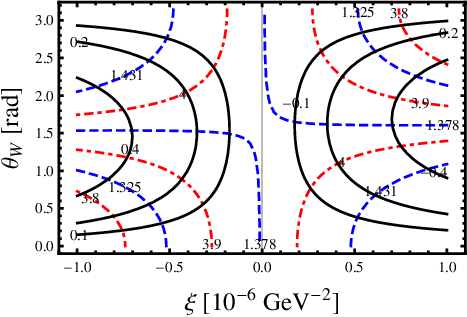
Since the involved parameters in Cabibbo allowed processes, $e.g.$, $D\to\pi K$, are different from the singly Cabibbo suppressed decays, with the assumption of $\sum_{i}f^{*}_{ic}f_{iu}\to 0$, the BRs for $D^{0}\to(\pi^{+}\pi^{-},K^{+}K^{-})$ are the potential constraint. Thus, we will take the data of the BRs with errors to constrain the free parameters. For Scheme I, we show the CPA difference defined in Eq. (6) as a function of $\xi\equiv\pm|f^{*}_{sc}f_{su}|/m^{2}_{H}$ and $\theta_{W}$ in Fig. 2. The solid lines correspond to the upper and lower bounds of the LHCb results. The dashed (blue) and dash-dotted (red) lines denote the experimental BRs for the decays $D^{0}\to(\pi^{+}\pi^{-},K^{+}K^{-})$, respectively. From these curves, we obtain the allowed region of the parameters as

Similarly, the results in Scheme II are presented in Fig. 3. In this scheme, we find that the magnitude of $\Delta A^{dir}_{CP}$ cannot fit the data within $1\sigma$ errors. The reason is that the direct CPA of $D^{0}\to\pi^{+}\pi^{-}$ in scheme II has the same sign with the one of $D^{0}\to K^{+}K^{-}$.

In order to understand the effects on each direct CPA $A^{dir}_{CP}$ defined in Eq. (7), by using Scheme I, we display $A^{dir}_{CP}$ for $D^{0}\to\pi^{+}\pi^{-}$ and $K^{+}K^{-}$ decays in Figs. 4a and 4b, respectively. The results, even the sign, are consistent with the current CDF data shown in Eq. (3).

In summary, it is clearly an exciting moment if any CPA in D-meson decays is observed at the percent level as the SM prediction is far below 1%. Motivated by the recent LHCb measurement on the time integrated CPA in $D^{0}\to(\pi^{+}\pi^{-},K^{+}K^{-})$ decays, which appears to be inconsistent with the SM result, we have studied the contributions of the colored scalar boson and used the color sextet $(6,1,1/3)$ as the illustrator. In this diqaurk model, the serious constraint from the D mixing parameter induced by box diagrams could be avoided if a cancellation among different flavor couplings occurs. We have found that the the induced direct CPAs of $D^{0}\to(\pi^{+}\pi^{-},K^{+}K^{0})$ decays can fit the recent LHCb results and are consistent with the CDF current measurement.

WW thanks Ahmed Ali for useful discussions. We are grateful to Prof. H. Y. Cheng for a communication. This work is supported by the National Science Council of R.O.C. under Grant #s: NSC-100-2112-M-006-014-MY3 (CHC) and NSC-98-2112-M-007-008-MY3 (CQG) and the Alexander von Humboldt Foundation (WW) .

References

- [1] R. Aaij et al. [LHCb Collaboration], arXiv:1112.0938 [hep-ex], to appear in Phys. Rev. Lett. See also Matthew Charles, LHCb Collaboration, talk presented at HCP2011 (Nov. 14–18, 2011, Paris, France), LHCb-CONF-2011-061, arXiv:1201.6268 [hep-ex].
- [2] T. Aaltonen et al. [CDF Collaboration], Phys. Rev. D 85, 012009 (2012) [arXiv:1111.5023 [hep-ex]].
- [3] D. Asner et al. [Heavy Flavor Averaging Group], arXiv:1010.1589 [hep-ex].
- [4] Online update athttp://www.slac.stanford.edu/xorg/hfag.
- [5] I. I. Bigi, A. Paul, and S. Recksiegel, J. High Energy Phys. 06 (2011) 089; I. I. Bigi and A. Paul, arXiv:1110.2862.
- [6] G. Isidori, J. F. Kamenik, Z. Ligeti and G. Perez, arXiv:1111.4987 [hep-ph].
- [7] J. Brod, A. L. Kagan and J. Zupan, arXiv:1111.5000 [hep-ph].
- [8] K. Wang and G. Zhu, arXiv:1111.5196 [hep-ph].
- [9] M. Gersabeck, M. Alexander, S. Borghi, V. VGligorov and C. Parkes, arXiv:1111.6515 [hep-ex].
- [10] A. N. Rozanov and M. I. Vysotsky, arXiv:1111.6949 [hep-ph].
- [11] Y. Hochberg and Y. Nir, arXiv:1112.5268 [hep-ph].
- [12] D. Pirtskhalava and P. Uttayarat, arXiv:1112.5451 [hep-ph].
- [13] H. -Y. Cheng and C. -W. Chiang, arXiv:1201.0785 [hep-ph].
- [14] B. Bhattacharya, M. Gronau and J. L. Rosner, arXiv:1201.2351 [hep-ph].
- [15] X. Chang, M. -K. Du, C. Liu, J. -S. Lu and S. Yang, arXiv:1201.2565 [hep-ph].
- [16] G. F. Giudice, G. Isidori and P. Paradisi, arXiv:1201.6204 [hep-ph].
- [17] W. Altmannshofer, R. Primulando, C. -T. Yu and F. Yu, arXiv:1202.2866 [hep-ph].
- [18] S. M. Barr and A. Zee, Phys. Rev. Lett. 55, 2253 (1985).
- [19] S. M. Barr, Phys. Rev. D34, 1567 (1986).
- [20] S. M. Barr and E. M. Freire, Phys. Rev. D41, 2129 (1990).
- [21] C. H. Chen, Phys. Lett. B 680, 133 (2009) [arXiv:0902.2620 [hep-ph]].
- [22] H. -Y. Cheng and C. -W. Chiang, Phys. Rev. D 81, 074021 (2010) [arXiv:1001.0987 [hep-ph]].
- [23] A. J. Buras, J. M. Gerard and R. Ruckl, Nucl. Phys. B 268, 16 (1986).
- [24] K. Nakamura et al. (Particle Data Group) J. Phys. G 37, 075021 (2010).
- [25] R. N. Mohapatra, N. Okada and H. B. Yu, Phys. Rev. D77, 011701 (2008) [arXiv:0709.1486 [hep-ph]].
- [26] T. Han, I. Lewis and Z. Liu, JHEP 1012, 085 (2010) [arXiv:1010.4309 [hep-ph]].