Symmetric Device-Independent Quantum Key Distribution Against General Attack

Quantum key distribution (QKD) is an art of generating physically secure key between remote partners, the information sender Alice, and the receiver Bob [1, 2, 3], even if in the presence of a powerful eavesdropper, namely Eve, whose capability is only limited by quantum mechanics. On one hand, the security proof of QKD has been obtained with nearly perfect apparatus [4, 5]. On the other hand, there are different loopholes in current QKD experiments that may injure the security of the final key bits [6, 7, 8, 9, 10, 11, 12]. Even with the perfect experimental apparatus [4, 5], there are also some self-evident assumptions that guarantee the security of final key bits. For instance, we have to assume that Alice and Bob have the freedom to choose the bases for their preparations and measurements. Their classical results which is unwanted to be leaked out should be completely secret. At the same time, Alice and Bob should entirely control their apparatus to generate the raw keys. Or else, the final key bits cannot be secure.

As for commercial application, the apparatuses of Alice and Bob will be black boxes that may be provided by their potential rivals. It is interesting how Alice and Bob can determine the security of their final key bits extracted from these black boxes? Recently, the device-independent QKD (DIQKD) [13, 14, 15] has been suggested to ask for the answer. It was assumed in this protocol that Alice and Bob have no knowledge about their measurement devices. The violation of CHSH inequality will impose restriction on Hilbert space dimension of their measurements to ensure the efficient quantum correlations between Alice and Bob [16, 17]. Secure key bits against collective attack for this protocol has been proven [14, 15]. Its final key generation rate depends on two parameters, the quantity of CHSH polynomial $S$ and the quantum bit error rate (QBER) $Q$. These two parameters are decided by the state measured by the legitimate users’ devices and the way of their measurements at the same time. As Alice and Bob have no idea about the state prepared by Eve, and their measurement devices can also be fabricated by their rivals, generalization from collective attack to general attack is still missed.

The way of state preparation in DIQKD is the same as those of Ekert91 protocol [2] and entanglement-based QKD protocol with sources in the middle [18, 19] where Eve’s eavesdropping ability is bounded with collective attack as quantum De Finetti theorem can be applied after Alice and Bob having randomized the measurement sequences on their states [20, 21]. In DIQKD, however, It is impossible for Alice and Bob to make sure that their measurements function exactly on the quantum systems as their expectations. In fact, Eve may devise Alice’s and Bob’s measurements differently in every run. In this paper, a symmetric DIQKD protocol is proposed. The symmetry of this protocol, together with the Holevo limit [22, 24, 23], will provide strong confinements on Eve’s eavesdropping. We show Eve’s information is maximized when all states distributed to Alice and Bob are identically prepared. Then the procedure of uniform their states is completed automatically, and Alice and Bob can estimate their parameters by randomizing the sequences of their classical results. Furthermore, Eve’s optimal state when her illegal information is maximized can be solely bounded with Alice and Bob’s parameter $S$. Then our symmetric DIQKD has the same secure basis as that of Ekert91 protocol.

Our DIQKD protocol is symmetric not only because Alice’s and Bob’s basis choices are symmetric, but also because the statistical results generated from all bases are the same. It works as follows. (1) $N$ EPR pairs emit from the signal source set between Alice’s and Bob’s labs. One particle of the EPR pair is sent to Alice and the other one is sent to Bob. (2) Both Alice and Bob choose four expecting measurement bases as $\theta_{1}=\sigma_{x}$, $\theta_{2}=(\sigma_{x}+\sigma_{z})/\sqrt{2}$, $\theta_{3}=\sigma_{z}$, $\theta_{4}=(-\sigma_{x}+\sigma_{z})/\sqrt{2}$ (As is shown in Fig. 1). In each run, Alice will randomly measure the incoming particle in one of the four bases, and so does Bob. (3) After all EPR pairs having been distributed, Alice and Bob announce the bases they used in each run through their classical channels. (4) Alice and Bob randomize the sequences of their classical results. They keep partial measurement results on the same bases as secrecy that will be used to generate secure final key bits. Then they publish all the other measurement results to estimate the disturbances and correlations on their sifted key bits. They abort their communication if the parameter estimation fails to meet their predefined requirements. Or else, they carry out privacy amplification to generate their secure final key.

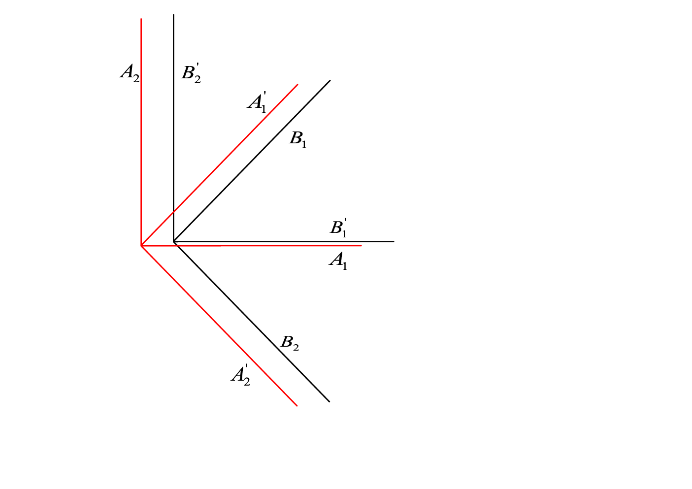
Without loss of generality, we assume Eve prepares all Alice’s and Bob’s systems and her auxiliary systems in a big state $\rho_{A_{1\cdots{N}}B_{1\cdots{N}}E}$. Noting Alice’s measurement operations as $A_{1}$, $A_{2}$, $A_{1}^{\prime}$ and $A_{2}^{\prime}$, Bob’s measurement operations as $B_{1}$, $B_{2}$, $B_{1}^{\prime}$ and $B_{2}^{\prime}$, the joint measurements of Alice’s and Bob’s devices can then be depicted as $A^{u_{1}}_{i_{1}}(t_{1})\otimes{B^{v_{1}}_{j_{1}}(t_{1})}\cdots{A^{u_{N}}_{i_{N}}(t_{N})}\otimes{B^{v_{N}}_{i_{N}}(t_{N})}$. Here $t_{1}$, $\cdots$, ${t_{N}}$ are sorted in time sequence as Eve may eavesdrop on Alice’s and Bob’s measurements differently in every run, $u_{1}$, $\cdots$, $u_{N}$, $v_{1}$, $\cdots$, $v_{N}$ correspond to the upper indexes, and $i_{1}$, $\cdots$, $i_{N}$ can be $1$ or $2$ randomly. As Eve’s measurements will not affect the marginal distributions of Alice’s and Bob’s classical results, their results generated from $\rho_{A_{1\cdots{N}}B_{1\cdots{N}}E}$ can be depicted as $Tr[A^{u_{1}}_{i_{1}}(t_{1})\otimes{B^{v_{1}}_{j_{1}}(t_{1})}\cdots{A^{u_{N}}_{i_{N}}(t_{N})}\otimes{B^{v_{N}}_{i_{N}}(t_{N})}Tr_{E}(\rho_{A_{1\cdots{N}}B_{1\cdots{N}}E})]$, where $Tr_{E}$ is the trace on Eve’s systems. According to DIQKD protocol, the result in the $k$th run is $Tr(A^{u_{k}}_{i_{k}}(t_{k})\otimes{B^{v_{k}}_{i_{k}}}(t_{k})(Tr_{A_{1\cdots{k-1}k+1\cdots{N}}B_{1\cdots{k-1}k+1\cdots{N}}E}(\rho_{A_{1\cdots{N}}B_{1\cdots{N}}E}))=a^{k}b^{k}$, where $a_{k}$ and $b_{k}$ are the classical results obtained by Alice and Bob respectively. If they are binary, taking $-1$ and $1$ for example, it is proven that $A^{u_{k}}_{i_{k}}(t_{k})$ and $B^{v_{k}}_{i_{k}}(t_{k})$ functioned on qubit states [14, 15, 25, 26, 27]. Furthermore, $A_{1_{k}}(t_{k})$, $A_{2_{k}}(t_{k})$, $B_{1_{k}}(t_{k})$ and $B_{2_{k}}(t_{k})$ can be set in the same plane $x-z$. Similarly, $A^{\prime}_{1_{k}}(t_{k})$, $A^{\prime}_{2_{k}}(t_{k})$, $B^{\prime}_{1_{k}}(t_{k})$ and $B^{\prime}_{2_{k}}(t_{k})$ can be set in another plane $x^{\prime}-z^{\prime}$ [14, 15].

Defining $Tr_{A_{1\cdots{k-1}k+1\cdots{N}}B_{1\cdots{k-1}k+1\cdots{N}}E}(\rho_{A_{1\cdots{N}}B_{1\cdots{N}}E})\equiv\rho^{k}_{AB}$, the Hilbert space of Alice and Bob as $H_{AB}$, $\rho^{k}_{AB}\in{H_{AB}}$ and dim$H_{AB}\leq 4$ should be satisfied. According to Holevo limit [22, 23, 24], Eve’s ability to distinguish the state shared by Alice and Bob is limited by $S(Tr_{E}(\rho_{A_{1\cdots{N}}B_{1\cdots{N}}E}))$, where $S(\rho)=-Tr(\rho\log_{2}(\rho))$ is the von Neumann entropy. If writing $\rho_{A_{1\cdots{N}}B_{1\cdots{N}}E}$ as $\rho_{A_{1\cdots{s}s+1\cdots{N}}B_{1\cdots{s}s+1\cdots{N}}E}$, $S(Tr_{E}(\rho_{A_{1\cdots{N}}B_{1\cdots{N}}E}))\leq{S(Tr_{A_{s+1\cdots{N}}B_{s+1\cdots{N}}E}(\rho_{A_{1\cdots{N}}B_{1\cdots{N}}E}))}+S(Tr_{A_{1\cdots{s}}B_{1\cdots{s}}E}(\rho_{A_{1\cdots{N}}B_{1\cdots{N}}E}))$ is required for the subadditivity of entropy. With the same procedure, one can have $S(Tr_{E}(\rho_{A_{1\cdots{N}}B_{1\cdots{N}}E}))\leq\sum_{k}S(Tr_{A_{1\cdots{k-1}k+1\cdots{N}}B_{1\cdots{k-1}k+1\cdots{N}}E}(\rho_{A_{1\cdots{N}}B_{1\cdots{N}}E}))$. The equality holds if and only if $Tr_{E}(\rho_{A_{1\cdots{N}}B_{1\cdots{N}}E})$ can be written as $N$ product systems shared between Alice and Bob, that is, $Tr_{E}(\rho_{A_{1\cdots{N}}B_{1\cdots{N}}E})=\otimes_{k=1}^{N}\rho^{k}_{AB}$.

Eve controls the transmission of quantum state, thus she can make $\rho^{k}_{AB}$ optimal for her information gain. As dim$H_{AB}\leq 4$, projective measurements can be launched on $\rho^{k}_{AB}$ in a 4-dimensional Hilbert space $H$, with $H_{AB}\subseteq{H}$. Let $\sum_{l}P^{l}_{AB}=I$ be projective measurements in $H$, it is proven that $S(\sum_{l}P^{l}\rho^{k}_{AB}P^{l})\geq{S(\rho^{k}_{AB})}$. The equality holds if and only if $\rho^{k}_{AB}=\sum_{l}P^{l}\rho^{k}_{AB}P^{l}$ [24]. That is, $\sum_{l}P^{l}\rho^{k}_{AB}P^{l}$ can be diagonalized in bases $T=\{\tau_{l}\}$ with $\tau_{l}\tau^{{\dagger}}_{l}=P^{l}$. Defining $\Lambda\equiv\sum_{l}P^{l}\rho^{k}_{AB}P^{l}=P^{-1}\rho^{k}_{AB}P$, then $\Lambda$ is a diagonal matrix in $H$, and $P$ is composed with the basis vectors $\{\tau^{k}\}$. Noticing Bell bases $B=\{\varsigma_{l}\}$ is also a set of bases in $H$, there should be a unitary operator $U$ satisfying $T=UB$. Then one can have $\Lambda=B^{-1}U^{-1}\rho^{k}_{AB}UB$, which means $\rho^{k}_{AB}$ can be diagonalized in Bell bases after it has been operated as $U^{-1}\rho^{k}_{AB}U$. It is apparently that this process will not alter the amount of entanglement on $\rho^{k}_{AB}$, and Eve’s information gain is only determined by the elements of $\Lambda$. That is, the assumption that the state $\rho^{k}_{AB}$ can be diagonlized on Bell bases will not affect Eve’s information gain, and at the same time, it will not harm Eve’s ability to intervene Alice and Bob’s communication. Then it does not loss any generality to assume $\rho^{k}_{AB}$ can be diagonalized on Bell bases so long as both Alice’s and Bob’s marginal distributions are symmetric [14, 15].

Suppose the state distributed by Eve in the $k$th run is $\sigma^{k}_{AB}\equiv(1-p_{k})\rho_{|\Phi^{+}\rangle}+p_{k_{1}}\rho_{|\Phi^{-}\rangle}+p_{k_{2}}\rho_{|\Psi^{+}\rangle}+p_{k_{3}}\rho_{|\Psi^{-}\rangle}$, where $p_{k}=p_{k_{1}}+p_{k_{2}}+p_{k_{3}}$, $|\Phi^{+}\rangle=\frac{1}{\sqrt{2}}(|00\rangle+|11\rangle)$, $|\Phi^{-}\rangle=\frac{1}{\sqrt{2}}(|00\rangle-|11\rangle)$, $|\Psi^{+}\rangle=\frac{1}{\sqrt{2}}(|01\rangle+|10\rangle)$, and $|\Psi^{-}\rangle=\frac{1}{\sqrt{2}}(|01\rangle-|10\rangle)$. We now show that Eve’s information on Alice and Bob’s results is maximized when all $\sigma^{k}_{AB}$s are identically prepared.

(I) When there are only two types of quantum states equiprobably prepared on Alice and Bob’s $N$ shared systems (This assumption does not loss any generality if these two states are prepared to be the same), they can be denoted as $\sigma^{(\alpha)}_{AB}=(1-p^{(\alpha)})\rho_{|\Phi^{+}\rangle}+p^{(\alpha)}_{1}\rho_{|\Phi^{-}\rangle}+p^{(\alpha)}_{2}\rho_{|\Psi^{+}\rangle}+p^{(\alpha)}_{3}\rho_{|\Psi^{-}\rangle}$ and $\sigma^{(\beta)}_{AB}=(1-p^{(\beta)})\rho_{|\Phi^{+}\rangle}+p^{(\beta)}_{1}\rho_{|\Phi^{-}\rangle}+p^{(\beta)}_{2}\rho_{|\Psi^{+}\rangle}+p^{(\beta)}_{3}\rho_{|\Psi^{-}\rangle}$. Then Eve’s information gain on these states should be represented as $\frac{N}{2}S(\sigma^{(\alpha)}_{AB})+\frac{N}{2}S(\sigma^{(\beta)}_{AB})$. If the statistical state on the $N$ entangled systems measured by Alice and Bob is $\sigma_{AB}=(1-p)\rho_{|\Phi^{+}\rangle}+p_{1}\rho_{|\Phi^{-}\rangle}+p_{2}\rho_{|\Psi^{+}\rangle}+p_{3}\rho_{|\Psi^{-}\rangle}$, we have $p^{(\alpha)}_{1}=p^{(\beta)}_{1}=p_{1}$, $p^{(\alpha)}_{2}=p^{(\beta)}_{2}=p_{2}$, and $p^{(\alpha)}_{3}=p^{(\beta)}_{3}=p_{3}$ when Eve’s information gain is optimal.

(II) When there are $m$ types of density matrixes equiprobably prepared by Eve, we assume Eve’s illegal information is maximal only when all of them are identically prepared on the $N$ entangled systems between Alice and Bob. That is, $S(\sigma^{(\alpha)}_{AB})+S(\sigma^{(\beta)}_{AB})+\cdots+S(\sigma^{(m)}_{AB})\leq{m}S(\sigma_{AB})$ is satisfied with the equality holds if and only if $\sigma^{(\alpha)}_{AB}=\sigma^{(\beta)}_{AB}=\cdots=\sigma^{(m)}_{AB}=\sigma_{AB}$. Here $\sigma_{AB}$ is the statistical expression on the $N$ shared systems of Alice and Bob.

(III) When there are $m+1$ types of states measured by Alice and Bob equiprobably, Eve’s information gain on them can be written as $S_{E}=\frac{N}{m+1}[S(\sigma^{(\alpha)}_{AB})+S(\sigma^{(\beta)}_{AB})+\cdots+S(\sigma^{(m)}_{AB})+S(\sigma^{(m+1)}_{AB})]$. If the statistical expression for the first $m$ types of states on the $\frac{m}{m+1}N$ systems is $\sigma^{(\Omega)}_{AB}=(1-p^{(\Omega)})\rho_{|\Phi^{+}\rangle}+p^{(\Omega)}_{1}\rho_{|\Phi^{-}\rangle}+p^{(\Omega)}_{2}\rho_{|\Psi^{+}\rangle}+p^{(\Omega)}_{3}\rho_{|\Psi^{-}\rangle}$, $S_{E}$ can be bounded as $\frac{N}{m+1}[mS(\sigma^{(\Omega)}_{AB})+S(\sigma^{(m+1)}_{AB})]$ according to step (II). With simple calculation, one can obtain its maximum value when $\sigma^{(\Omega)}_{AB}=\sigma^{(m+1)}_{AB}=\sigma_{AB}$, with $\sigma_{AB}$ being the statistical representation of all $N$ shared systems between Alice and Bob. In conclusion, Eve should prepare the state on the $N$ systems identically if she want to maximize her illegal information from Alice and Bob’s communication. Then there is no need to randomize the measurement sequences to make their states uniformly distributed. Quantum De Finetti theorem can be applied in DIQKD protocol and Eve’s information can be bounded with collective attack [20, 21].

Alice and Bob may not infer Eve’s single intervention on their measurements in the $k$th run because of quantum randomness. As their states are identically prepared, however, they can deduce the equivalent operations averaged from all results. Denoting the equivalent operations in $x-z$ plane as $A_{1}$, $A_{2}$, $B_{1}$ and $B_{2}$, their directions are assumed to be $\theta_{1}$, $\theta_{2}$, $\varphi_{1}$ and $\varphi_{2}$ respectively. Similarly, denoting the equivalent operations in $x^{\prime}-z^{\prime}$ plane as $A^{\prime}_{1}$, $A^{\prime}_{2}$, $B^{\prime}_{1}$ and $B^{\prime}_{2}$, the corresponding directions for them are $\theta^{\prime}_{1}$, $\theta^{\prime}_{2}$, $\varphi^{\prime}_{1}$ and $\varphi^{\prime}_{2}$. The CHSH polynomial can be calculated as $S=\sum_{i,j}{sign(3.5-i-j)}Tr(A_{i}B_{j}\sigma_{AB})$, and $S^{\prime}=\sum_{i,j}{sign(3.5-i-j)}Tr(A^{\prime}_{i}B^{\prime}_{j}\sigma_{AB})$, with $i$, $j=1$, or $2$, and $sign(x)$ getting the sign of $x$. Our symmetric DIQKD protocol requires $S=S^{\prime}$, moreover, it requires that all $sign(3.5-i-j)Tr(A_{i}B_{j}\sigma_{AB})$s and $sign(3.5-i-j)Tr(A^{\prime}_{i}B^{\prime}_{j}\sigma_{AB})$s have the same value $\frac{S}{4}$. Then one can obtain $p_{1}=p_{2}$, and $\theta_{2}-\theta_{1}=\frac{\pi}{2}$, $\varphi_{2}-\varphi_{1}=-\frac{\pi}{2}$, $\theta_{2}-\varphi_{1}=\frac{\pi}{4}$ and $\theta_{1}-\varphi_{2}=\frac{\pi}{4}$, or $\theta_{2}-\theta_{1}=-\frac{\pi}{2}$, $\varphi_{2}-\varphi_{1}=\frac{\pi}{2}$, $\theta_{2}-\varphi_{1}=-\frac{\pi}{4}$ and $\theta_{1}-\varphi_{2}=-\frac{\pi}{4}$. With the same procedure, we can have the relationships among $\theta^{\prime}_{1}$, $\theta^{\prime}_{2}$, $\varphi^{\prime}_{1}$ and $\varphi^{\prime}_{2}$. It is interesting to find that measurements satisfying the above relationships can be proven to maximize the value of $S$. For Alice and Bob, bigger $S$ means less disturbances, then Eve should have the measurements of Alice and Bob in every run obeys the above relationships in order to conceal her existence.

Two important things may be reconsidered: what is the relationship between plane $x-z$ and $x^{\prime}-z^{\prime}$ and whether should Eve prepares the states for $A_{1}$, $A_{2}$, $B_{1}$, $B_{2}$ and $A_{1}^{\prime}$, $A_{2}^{\prime}$, $B_{1}^{\prime}$, $B_{2}^{\prime}$ with different systems? It is interesting to notice that both questions deal with the relationship between measurements and information. And they can be answered at the same time. If plane $x-z$ does not coincide with plane $x^{\prime}-z^{\prime}$, they belong to different Hilbert spaces. When Eve prepares the states on the same systems, generalized measurements are carried out inevitably when Eve distributes them in two different Hilbert spaces. This process will decrease Eve’s information gain on the state [24]. However, when Eve prepares the states on plane $x-z$ and $x^{\prime}-z^{\prime}$ with different systems, monogamy of entanglement means that Alice’s and Bob’s results extracted on the same bases should be totally uncorrelated [28, 29, 30]. This will increase QBER on the key, that is, she will risk to be detected on line without gaining more information. Then for the sake of Eve’s optimal information gain, and concealing her existence at the same time, the Hilbert space of $x-z$ coincides with that of $x^{\prime}-z^{\prime}$, and the states for them are prepared on the same systems correspondingly.

When $p_{1}=p_{2}$, one can have the relationship $p_{1}+p_{3}=\frac{1}{2}-\frac{S}{4\sqrt{2}}$. If the measurement directions between Alice and Bob are well aligned, the QBER can be calculated as $p_{1}+p_{3}$. Or else, it should be written as $Q=\frac{1-(1-p-p_{3})\cos\vartheta}{2}$, where $\vartheta$ is the included angle between these measurement directions. This value is greater than that of the former. Then Alice’s measurement bases should keep alignment with those of Bob, one can obtain $S=2\sqrt{2}[1-2Q]$, which is the same as that in [14, 15]. In practical implementation of DIQKD, Alice and Bob can not obtain the value of $p$. Defining $q\equiv{p+p_{3}}$, we have $q=1-\frac{S}{2\sqrt{2}}=2Q$. But the exact value of $p_{1}$ and $p_{3}$ is still unknown. As Eve’s information on $\sigma_{AB}$ can be written as $S(\sigma_{AB})=-(1-q+p_{3})\log_{2}(1-q+p_{3})-2p_{1}\log_{2}p_{1}-p_{3}\log_{2}p_{3}$, however, we have $p_{3}=\frac{q^{2}}{4}$ and $p_{1}=\frac{q}{2}-\frac{q^{2}}{4}$ when $S(\rho_{AB})$ is maximal. That is, the optimal state for Eve’s eavesdropping is $\sigma^{optimal}_{AB}=(1-q+\frac{q^{2}}{4})\rho_{|\Phi^{+}\rangle}+(\frac{q}{2}-\frac{q^{2}}{4})\rho_{|\Phi^{-}\rangle}+(\frac{q}{2}-\frac{q^{2}}{4})\rho_{|\Psi^{+}\rangle}+\frac{q^{2}}{4}\rho_{|\Psi^{-}\rangle}$. Different to the cases where Alice and Bob having full control of their measurement devices [31, 32, 33], color noise is optimal for Eve in the DIQKD protocol. This is because Alice and Bob can calculate the value of $p$ accurately in the former but they can only estimate the value of $q$ in the latter.

Until to now, we have proven Eve’s optimal information to be $S(\sigma^{optimal}_{AB})$. If its corresponding quantity of CHSH polynomial is $S^{optimal}$, however, can Eve’s optimal information be bounded as $S(\sigma^{optimal}_{AB})$ when Alice and Bob’s statistical value of $S$ is equal to $S^{optimal}$? If not so, there must be another $\sigma^{optimal\prime}_{AB}$ with which Eve can obtain more illegal information. That is, $S(\sigma^{optimal\prime}_{AB})>S(\sigma^{optimal}_{AB})$ is satisfied. According to the discussion above, $\sigma^{optimal\prime}_{AB}$ should also be represented as $\sigma^{optimal\prime}_{AB}=(1-q^{\prime}+\frac{q^{\prime 2}}{4})\rho_{|\Phi^{+}\rangle}+(\frac{q^{\prime}}{2}-\frac{q^{\prime 2}}{4})\rho_{|\Phi^{-}\rangle}+(\frac{q^{\prime}}{2}-\frac{q^{\prime 2}}{4})\rho_{|\Psi^{+}\rangle}+\frac{q^{\prime 2}}{4}\rho_{|\Psi^{-}\rangle}$. Its corresponding $S$ can be calculated to be less than $2\sqrt{2}(1-q^{\prime})$. As $S(\sigma^{optimal\prime}_{AB})>S(\sigma^{optimal}_{AB})$, one can have ${S^{optimal}}\leq 2\sqrt{2}(1-q^{\prime})\leq 2\sqrt{2}(1-q)$. For Alice and Bob, great $S$ means less information can be obtained Eve, which means $S^{optimal}$ can bound Eve’s illegal information. Generally, if the value of CHSH polynomial is $S$, Eve’s illegal information should be less than $E(S)=-\frac{1}{4}(1+\frac{S}{2\sqrt{2}})\log_{2}\frac{1}{4}(1+\frac{S}{2\sqrt{2}})-\frac{1}{4}(1-\frac{S}{2\sqrt{2}})\log_{2}\frac{1}{4}(1-\frac{S}{2\sqrt{2}})-(\frac{1}{2}-\frac{S^{2}}{16})\log_{2}(\frac{1}{4}-\frac{S^{2}}{32})$. Thus, DIQKD can be bounded with the quantity of CHSH polynomial, which means it has the same secure basis as that of Ekert91 protocol [2]. For collective attack, Alice and Bob’s key generation can be represented as $r=1-H_{2}(Q)-\chi$, where $H_{2}(Q)=-Q\log_{2}Q-(1-Q)\log_{2}(1-Q)$ is the Shannon entropy and $\chi$ is the Holevo limit [34, 35]. In our symmetric DIQKD, the lower bound of Alice and Bob’s key generation rate can be estimated as $r\geq 1-H_{2}(Q)-S(\sigma^{optimal}_{AB})$. If the relationship $S=2\sqrt{2}(1-2Q)$ is satisfied, the key rate of our DIQKD can be calculated as

In this paper, a symmetric DIQKD has been proposed, where Eve’s ability of eavesdropping can be bounded with collective attack. That is, generalization on the security of DIQKD from collective attack to general attack can be realized. Its security can be estimated similarly as that of Ekert91 protocol, that is, determined by the quantity of CHSH polynomial $S$. However, we have only considered an ideal case where the loss in the quantum channel is not added in. In practical implementation of this protocol, there may be detecting loophole because of imperfectly detecting efficiency [32, 33]. Especially, faking state attack has been proposed to eavesdrop on DIQKD protocols with inefficient measurement devices [36]. To make DIQKD more practically with present devices, however, proposition for experimental realization of this protocol has been given [37]. Besides its attractiveness of practical application, DIQKD is physically interesting as it provides us a way to understand the nonlocality of quantum principles, with which the legitimate users can set up secure communication without any knowledge about their quantum objects. The author thank helpful discussion from Q.-Y. Cai and X. Ma. This work is sponsored by the National Natural Science Foundation of China (Grant No 10905028) and HASTIT.

References

- [1] C. H. Bennett and G. Brassard, in Proceedings of the IEEE International Conference on Computers, Systems and Signal Processing, Bangalore, India (IEEE, New York), PP. 175 (1984).
- [2] A. K. Ekert, Phys. Rev. Lett. 67, 661 (1991).
- [3] N. Gisin, G. Ribordy, W. Tittel, and H. Zbinden, Rev. Mod. Phys. 74, 145 (2002).
- [4] H.-K. Lo and H. F. Chau, Science 283, 2050¨C2056 (1999).
- [5] P. W. Shor and J. Preskill, Phys. Rev. Lett. 85, 441 (2000).
- [6] B. Huttner, N. Imoto, N. Gisin and T. Mor, Phys. Rev. A 51, 1863 (1995).
- [7] B. Qi, C.-H. F. Fung, H.-K. Lo and X. Ma, Quant. Inf. Comp. 7, pp. 73-82 (2007).
- [8] Y. Zhao, C.-H. F. Fung, B. Qi, C. Chen and H.-K. Lo, Phys. Rev. A 78, 042333 (2008).
- [9] C.-H. F. Fung, B. Qi, K. Tamaki and H.-K. Lo, Phys. Rev. A 75, 032314 (2007).
- [10] F. Xu, B. Qi and H.-K. Lo, New J. Phys. 12, 113026 (2010).
- [11] L. Lydersen, C. Wiechers, C. Wittmann, D. Elser, J. Skaar and V. Makarov, Nature Photonics 4, pp. 686-689 (2010); Z. L. Yuan, J. F. Dynes and A. J. Shields, Nature Photonics 4, pp. 800-801 (2010); L. Lydersen, C. Wiechers, C. Wittmann, D. Elser, J. Skaar and V. Makarov, Nature Photonics 4, 801 (2010).
- [12] I. Gerhardt, Q. Liu, A. Lamas-Linares, J. Skaar, C. Kurtsiefer and V. Makarov, Nature Comm. 2, 349 (2011).
- [13] D. Mayers and A. C.-C. Yao, in Proceedings of the 39th Annual Symposium on Foundations of Computer Science (FOCS98), (IEEE Computer Society, Washington, DC, 1998), p. 503.
- [14] A. Acín, N. Brunner, N. Gisin, S. Massar, S. Pironio and V. Scarani, Phys. Rev. Lett. 98, 230501 (2007);
- [15] S. Pironio, A. Acín, N. Brunner, N. Gisin, S. Massar and V. Scarani, New J. Phys. 11, 045021 (2009).
- [16] J. Clauser et. al., Phys. Rev. Lett. 23, 880 (1969).
- [17] J. S. Bell, Phsycis 1, 195 (1965).
- [18] X. Ma , C.-H. F. Fung , and H.-K. Lo, Phys. Rev . A 76 012307, (2007).
- [19] R. Renner, N. Gisin, B. Kraus, Phys. Rev. A 72, 012332 (2005).
- [20] R. Renner, Ph.D. thesis, ETH No. 16242, arXiv:quant-ph/ 0512258.
- [21] R. Renner, Nature Phys. 3, 645 (2007).
- [22] A. S. Holevo, Probl. Peredachi. Inf., 9, 3 (1973).
- [23] A. Cabello, Phys. Rev. Lett., 85, 5635 (2000).
- [24] M. A. Nielsen, and I. L. Chuang, Quantum computation and quantum information. Cambridge University Press, (2000).
- [25] B. S. Tsirelson . Lett. Math. Phys., 4, 93 (1980).
- [26] B. Tsirelson, Hadronic Journal Supplement, 8, 329 (1993).
- [27] L. Masanes, Phys. Rev . Lett., 97, 050503 (2006).
- [28] D. Bruß, Phys. Rev. A, 60, 4344 (1999).
- [29] V. Coffman, J. Kundu, and W. K. Wootters, Phys. Rev. A, 61 052306 (2000).
- [30] M. Koashi, and A. Winter, Phys. Rev. A 69, 022309 (2004).
- [31] P. H. Eberhard, Phys. Rev. A, 47, R747 (1993).
- [32] N. Brunner, N. Gisin, V. Scarani, and C. Simon, Phys. Rev. Lett., 98, 220403 (2007).
- [33] A. Cabello and J.-A. Larsson, Phys. Rev. Lett. 98, 220402 (2007).
- [34] E. Biham and T. Mor, Phys. Rev. Lett., 79, 4034 (1997).
- [35] E. Biham and T. Mor. Phys. Rev. Lett., 78, 2256 (1997).
- [36] I. Gerhardt, Q. Liu, A. Lamas-Linares, J. Skaar, V. Scarani, V. Makarov, and C. Kurtsiefer, Phys. Rev. Lett., 107, 170404 (2011).
- [37] N. Gisin, S. Pironio, and N. Sangouard, Phys. Rev. Lett., 105, 070501 (2010).
Appendix A Bounding Eve’s information with Holevo limit
In DIQKD, Alice and Bob measure on the state prepared by Eve. According to the Holevo limit, Eve’s illegal information on the results of Alice and Bob can be bounded with . If is composed with many subsystems, that is, . can be proven to satisfy the relationship