Discontinuous Percolation Transitions in Epidemic Processes, Surface Depinning in Random Media and Hamiltonian Random Graphs
Abstract
Discontinuous percolation transitions and the associated tricritical points are manifest in a wide range of both equilibrium and non-equilibrium cooperative phenomena. To demonstrate this, we present and relate the continuous and first order behaviors in two different classes of models: The first are generalized epidemic processes (GEP) that describe in their spatially embedded version – either on or off a regular lattice – compact or fractal cluster growth in random media at zero temperature. A random graph version of these processes is mapped onto a model previously proposed for complex social contagion. We compute detailed phase diagrams and compare our numerical results at the tricritical point in with field theory predictions of Janssen et al. [Phys. Rev. E 70, 026114 (2004)]. The second class consists of exponential (“Hamiltonian”, i.e. formally equilibrium) random graph models and includes the Strauss and the 2-star model, where ‘chemical potentials’ control the densities of links, triangles or 2-stars. When the chemical potentials in either graph model are , the percolation transition can coincide with a first order phase transition in the density of links, making the former also discontinuous. Hysteresis loops can then be of mixed order, with second order behavior for decreasing link fugacity, and a jump (first order) when it increases.
pacs
64.60.ah, 68.43.Jk, 89.75.DaI Introduction
Percolation describes the sudden appearance of system-wide connectivity arising from microscopic processes. It is a classic example [1] of a continuous (“second order”) phase transition. Interest in systems where the percolation transition is discontinuous (“first order”) was sparked recently by claims for this in Achlioptas processes [2]. Although these transitions were later shown to be continuous [3, 4, 5, 6] – albeit with unusual finite size scaling behavior [5], the fact that percolation transitions could be discontinuous was claimed to be novel or even revolutionary [7, 8, 9, 10, 11, 12, 13, 14, 15, 16, 17, 18, 19, 20, 21, 22, 23, 24, 3, 4]. After this, discontinuous percolation transitions were observed in interdependent networks [25, 26, 7], in models inspired by [2] but not using the Achlioptas trick [15, 16, 17, 18], and in a hierarchical lattice [28].
One purpose of this work is to point out that discontinuous percolation transitions are not surprising and, indeed, are common to a variety of (e.g. social or physical) cooperative phenomena. The existence of such transitions, together with an associated tricritical point, was proposed 25 years ago [29] in the context of directed percolation. This was verified in the seminal field theoretic work of Janssen et al. [3] who introduced the generalized epidemic process (GEP) 11 1 Janssen et al. called this the ’generalized general epidemic process’ (GGEP), in order to distinguish it from the ’general epidemic process’ [D. Mollison, J. Royal Statist. Soc. B 39, 283 (1977)]. The latter is now usually called an SIR (susceptible-infected-removed) epidemic, while a ’simple epidemic’ in the notation of Mollison is now called SIS. We feel thus free to use the simpler acronym GEP for the generalized process.. In this scenario, the continuous transition is just ordinary percolation (OP), whilst the discontinuous one is the depinning transition of driven surfaces in random media at zero temperature [31, 32, 33, 34, 35, 36, 37].
Although the latter is continuous from the point of view of surface properties, it is discontinuous so far as the percolation order parameter is concerned 22 2 Note that the co-appearance of first order bulk transitions with continuous surface transitions was discussed already in [38].. Indeed, the density of ‘wetted’ sites in the presence of a driven interface jumps discontinuously from zero to a finite value at depinning.
A closely related line of papers finding discontinuous percolation transitions started independently in a social science context [39, 4, 41] and addresses complex contagion or epidemics in random networks. It turns out that the model of [4] is basically the random graph version of the GEP, as we explain in detail below. Our unified formulation based on GEP, that includes both social contagion and interface depinning, simplifies the description of both and isolates relevant variables that can affect the actual outcome in terms of potentially measurable observables.
We present numerical simulation results for the GEP, including the time dependence of the number of growth sites in three dimensions. At the first order (= depinning) transition line, activity decays as a stretched exponential in time whilst it behaves as a power-law both at the OP transition and at the tricritical point which separates rough from fractal growth. We give (tri-)critical exponents and compare them to theoretical predictions [3].
The main property that leads to first order transitions in the models we consider is cooperativity (or ‘synergy’) in establishing links. This cooperativity can be implemented technically in different ways. We do this via stochastic dynamics as in [3, 39, 4, 41] for the GEP, and also via Gibbs-Boltzmann equilibrium distributions in Hamiltonian (or “exponential”) ensembles, which have been used extensively to model social networks.
Indeed, we also find discontinuous percolation transitions in two exponential random graph models : the Strauss [42, 9] and the 2-star model [44]. They are both formulated in terms of a partition function and are generalizations of the standard Erdös-Renyi (ER) random graph [8]. The Hamiltonians are bilinear with a control parameter () conjugate to the number of links and another control parameter conjugate to either the number of triangles or the number of “2-stars.” When all control parameters are (where is the number of nodes in the graph), the percolation transition can be either continuous or discontinuous, with hysteresis loops typical of first-order transitions. But for certain parameter regimes unusual hysteresis loops occur, where the percolation order parameter exhibits second-order (singular but continuous) behavior for decreasing , but jumps discontinuously for increasing . Such “mixed-order” hysteresis loops have not to our knowledge been seen before.
It is well known that the observation of continuity of a phase transition depends not only on the choice of the order parameter, but also on the choice of the control parameter. Take e.g. the standard example of a liquid-gas transition. If the temperature of water is increased at constant pressure, then the density and the free energy jump discontinuously at the boiling temperature. If, however, the volume is kept fixed, no such jump is observed. Instead, as temperature is increased, a larger and larger fraction of the sample turns into vapor, but this happens in a completely continuous way. The standard assumption in thermostatics is that the order parameter is a density or inverse density (e.g. specific volume), and the control parameter is its conjugate (e.g. pressure). But in percolation, the standard choice of order parameter is the fraction of sites belonging to the giant cluster, while the control parameter is usually also a density – the density of occupied sites (bonds) in site (bond) percolation. Although this choice is legitimate, it can obscure the notion of first vs. second order transitions, since other choices more in line with thermostatics can lead to different conclusions. This might explain why previous works on first order percolation transitions were not recognized as such in the recent literature.
II The Generalized Epidemic Model: Complex Contagion Treated as a Stochastic Process
Although the epidemic model of Ref. [3] is formulated as a continuum field theory, the situation becomes more clear on a lattice. Consider a process where the probability of a given site becoming infected (or invaded) by one of its neighbors depends on the number of previous attempts by other neighbors. Once a site is infected, it tries once to infect every one of its not yet infected neighbors. Denote by the probability that an infection succeeds, if the attacked site has already fended off previous attacks. If every attack increases the strength of the defender, decreases with , otherwise (if it weakens it), increases. Site percolation is described by and for : If the first attack does not succeed, all later attempts are futile. Bond percolation is described by for all . Ordinary (second order) percolation is observed whenever decreases with (see also [46]), but the transition switches to first order when increases sufficiently fast. In that case, infected clusters fill in most holes and bays, while protrusions are avoided – thereby making the clusters compact with rough but non-fractal surfaces. (The same effect is caused by high surface tension compared to disorder at the cluster-void interface in random media). Detailed predictions for the tricritical behavior in terms of an expansion were given in [3].
II.1 The GEP on Random Graphs
Although Dodds et al. [4, 41] assume a somewhat more complex mechanism of infection, their basic model can be mapped onto a sparse random graph model where each node with neighbors in the the giant cluster is itself in the giant cluster with probability . This is precisely the mean field (random graph) version of the above model, if and 33 3 Strictly spoken this is only true for static (i.e., percolation in the narrow sense) aspects at threshold. Dynamics and the behavior above the threshold are different in both models, since the memory about previous contacts with infected neighbors is short lived in [4, 41], while it is long lived (previous attacks are never forgotten) in the model of [3] and in the simulations reported in the next subsection.. Due to the absence of short loops in this case, the condition for tricriticality (transition between classes I and II in [4, 41]) simplifies to
| (1) |
with no restriction on any with . Since the derivation of this in [4, 41] is somewhat involved and obscures the relationship to the GEP as defined in [3], a simple proof of Eq.(1) is given in the supplementary material.
II.2 The GEP on Regular Lattices: Tricritical Behavior and Rough Pinned Surfaces
In the present work we studied in detail the case where is the same for all , while is different. Phase diagrams for simple (hyper-) cubic lattices and for random regular graphs are shown in Fig. 1. To the left of the curves, no infinite clusters exist, while such clusters do exist to their right. Since percolation thresholds on lattices scale as for large , we used and as coordinates in Fig. 1, where is the coordination number. All curves start at site percolation (), since we do not consider here antagonistics effects (i.e., two attacks together cannot have less success than a single one). Tricritical points are marked by circles. There is no tricricital transition in [37], i.e. isotropic rough 1- surfaces are always fractal. For large dimensions, the lattice results converge to those for regular random graphs with degree , as short loops become less and less important with increasing . Preliminary results indicate that surface properties in the first-order regimes (i.e. below the tricritical points, but for ) are not in the same universality class of surfaces without overhangs, which is the accepted theory for pinned rough surfaces [47, 48, 49], while the situation is less clear in the case , i.e. if at least two infected neighbors are needed for a site to become infected (in the latter case, epidemics can neither spread from single sites nor from surfaces, but they can spread from surfaces).


For the simple cubic lattice, simulations show that the tricritical point for this model is at at and for . Results of such simulations for epidemics starting from a single infected site are shown in Fig. 2, where is the number of sites newly infected at time . For OP, increases as a power law with [1], it decreases at the tricritical point as with . This is in stark contrast to the prediction of [3]. The tricritical point and OP are the only cases where shows a power law. For critical percolation with the behavior crosses over to the OP scaling, while for the data are compatible with a stretched exponential at the transition line (see lowest three curves in Fig. 2). Analogous plots for the probability that the epidemic survives at least time steps and for its average squared radius are given in the supplementary material. They give and , where and are defined via and . The predictions of [3] are and . Again the agreement is far from perfect, although the changes from the OP critical exponents are in the right directions. More details are given in the supplementary material and in [2]. For the completely analogous case of directed percolation (SIS epidemics), see [51, 52, 53].
III Cooperative Percolation in Hamiltonian Random Graph Models
The above discussion suggests that cooperativity in finite temperature equilibrium systems may also lead to discontinuous percolation transitions. Indeed, the mean field percolation transition corresponds to the emergence of the giant component in ER random graphs, where links appear independently with probability [8]. The latter is the simplest “exponential model” [54, 55, 56]. In this approach one considers graphs with nodes, were the probability for a given graph is defined by the Boltzmann-Gibbs equilibrium formula
| (2) |
with . Here is the Hamiltonian, represents a set of control parameters, and we have set . More precisely, we assume that is a sum of bilinear terms,
| (3) |
where each is an observable (“statistic”) of the graph, and is the associated chemical potential. Typically, each represents the total number of small subgraphs (links, triangles, -stars, 4-cliques, …) in the graph.
Models of this type have been popular in mathematical sociology [42, 56], although they tend to be unrealistic. In many cases, such models reduce to equivalent ER graphs without clustering and are trivial, apart from the usual, non-trivial dependence of the observables on the control parameters [57].
The Hamiltonian for the ER model is:
| (4) |
where is the number of links in and . It exhibits a percolation transition at (when ) [8], thus the critical value of is
| (5) |
In the following, we study the 2-star model [44] with
| (6) |
Here is the total number of “2-stars”, i.e. of pairs of links attached to the same node. We also consider the Strauss model [42, 9] with
| (7) |
where is the total number of distinct triangles, i.e. of loops of length 3. In terms of the degree sequence ,
| (8) |
while depends also on degree correlations.
For a typical (non-sparse) graph increases quadratically with , while both and . This is why and are used as control parameters in Eqs. (6,7) instead of and . The 2-star model has, for any , a first order transition in the density of links at and strong hysteresis. The results of [44], together with a standard Maxwell construction show that
| (9) |
The line of first order transitions terminates at the critical point . (We neglect here all terms that are relative to the leading ones). Similarly, for the Strauss model a first order transition in the link density occurs for any [9]. This time it is more complicated to obtain the exact transition line , but one can show that (see Supplementary Material)
| (10) |
with a critical point at , and .
For both models, a giant component exists in both the high and low link density phases, whenever . Thus the density transition happens when they are already percolating, as long as is finite. In order to reach a percolation transition one has to take to get a sparse graph. In this regime the above estimates for the density transitions are still valid. Moreover, when or , respectively, the second terms in the Hamiltonians (Eqs. (6,7)) have no influence on the percolation transition, for . This is illustrated for the 2-star model in Fig. 2, where we show numerical results averaged over 50 hysteresis loops for a network with and . The density transition (monitored via the average degree) indeed appears to be first order with strong hysteresis, while the percolation transition (monitored via ) shows no hysteresis and is exactly the same as for ordinary ER networks.


When (or , respectively) this scenario breaks down because the true equilibrium state at the ER percolation threshold, , is a dense graph that consists of a single giant component. Although the equilibrium network percolates at , a hysteresis loop starting at begins with a sparse non-percolating graph, and due to metastability the effect of (or ) is not seen until one passes the ER percolation threshold – provided that it remains in the metastable region. This scenario is illustrated in Fig. 2 for . Now the hysteresis loop for is quite wide. The hysteresis loop for shows the ordinary ER percolation shape on its lower branch, while it follows the discontinuous behavior of on the upper (return) branch. To our knowledge, such a mixed-order hysteresis loop has not been observed before.
IV Conclusions
As we already mentioned and as was pointed out repeatedly before [44, 9, 57], the 2-star and Strauss models are not realistic for real world applications. Accordingly, our demonstration that they exhibit both second and first order percolation transitions should be considered only as a proof that this phenomenon exists in equilibrium. More interesting examples can be easily suggested. A class of models that come into mind are random graphs (i.e. mean field type) where not only the number of nodes but also the number of links is set by hard constraints (“microcanonical models”). A model with two control parameters ( and ) studied in [58] exhibits zoo of metastable states, but it seems that most of these states are still too extreme to be physical. A further step in this direction could be to fix not only the average degree, but to fix the entire degree distribution, either by soft [59] or by hard [60] constraints.
A more realistic class of Hamiltonian models with first order phase transitions could be spatially embedded (e.g. finite dimensional lattice) systems. Such models have not been studied much in the social science literature, although it is well-known that, for instance, spatial structure is essential to maintain diversity in ecosystems. We believe that such models might provide a suitable mixture of structure and randomness to reveal important features of real, complex networks, including presumably percolation transitions of both continuous and discontinuous type.
In summary, we have shown that various percolation models can be naturally generalized such that they switch from ordinary, continuous behavior at the transition point to discontinuous (“first order”) behavior, as some parameter is varied. This parameter usually is a measure of cooperativity in linking or “infecting” sites (the probability for sites to get linked is increased by other links already present), such that the percolation transition is more abrupt when cooperativity is high. We present a unified treatment including examples that range from social dynamics to condensed matter physics, and we also show that analogous phenomena occur both in stochastic dynamics out of equilibrium as well as in a Gibbs-Boltzmann equilibrium framework. We also simplify the dynamical description of the social contagion process introduced by Dodds and Watts [4], clarifying thereby its relation to percolation and to the generalized epidemic process defined in [3].
In condensed matter physics, the first order percolation transition is just the depinning transition of driven interfaces in disordered media at zero temperature. Treating it also in our unified framework not only allows us to study in detail the tricritical point (where we found for striking disagreement with theoretical predictions), but also to numerically investigate more efficiently a model for pinned surfaces in which overhangs are fully included and hence the rotational symmetry of the growth process is not explicitly broken at scales much less than the system size. In this latter context, the most important (but so far only preliminary) result we find is that overhangs are indeed crucial for such surfaces, and that all existing theories for critically pinned rough surfaces (which neglect overhangs and are based on a single-valued ”height function”) might be obsolete, not being relevant to the most interesting physical case of isotropic media.
References
- [1] D. Stauffer and A. Aharony, Introduction to Percolation Theory (Taylor & Francis, London, 1994)
- [2] D. Achlioptas, R. M. D’Souza, and J. Spencer, Science 323, 1453 (2009)
- [3] R. A. da Costa et al., Phys. Rev. Lett. 105, 255701 (2010)
- [4] O. Riordan and L. Warnke, Science 333, 322 (2011)
- [5] P. Grassberger, C. Christensen, C. Bizhani, S.-W. Son, and M. Paczuski, Phys. Rev. Lett. 106, 225701 (2011)
- [6] H. K. Lee, B. J. Kim, and H. Park, Phys. Rev. E 84, 020101(R) (2011)
- [7] A. Vespignani, Nature 464, 984 (2010)
- [8] E. J. Friedman and A. S. Landsberg, Phys. Rev. Lett. 103, 255701 (2009)
- [9] R. M. Ziff, Phys. Rev. Lett. 103, 045701 (2009)
- [10] R. M. Ziff, Phys. Rev. E 82, 051105 (2010)
- [11] F. Radicchi and S. Fortunato, Phys. Rev. Lett. 103, 168701 (2009)
- [12] F. Radicchi and S. Fortunato, Phys. Rev. E 81, 036110 (2010)
- [13] R. M. D’Souza and M. Mitzenmacher, Phys. Rev. Lett. 104, 195702 (2010)
- [14] H. D. Rozenfeld, L. K. Gallos, and H. A. Makse, Eur. Phys. J. B 75, 305 (2010)
- [15] S. S. Manna and A. Chatterjee, Physica A 390, 177 (2011)
- [16] A. A. Moreira, E. A. Oliveira, S. D. S. Reis, H. J. Herrmann, and J. S. Andrade, Phys. Rev. E 81, 040101(R) (2010)
- [17] N. A. M. Araújo and H. J. Herrmann, Phys. Rev. Lett. 105, 035701 (2010)
- [18] W. Chen and R. M. D’Souza, Phys. Rev. Lett. 106, 115701 (2011)
- [19] Y. S. Cho, B. Kahng, and D. Kim, Phys. Rev. E 81, 030103 (2010)
- [20] Y. S. Cho et al., Phys. Rev. Lett. 103, 135702 (2009)
- [21] Y. S. Cho et al., Phys. Rev. E 82, 042102 (2010)
- [22] L. Tian and D.-N. Shi, arXiv: 1010.5990 (2010)
- [23] J. Nagler, A. Levina, and M. Timme, Nature Phys. 7, 265 (2011)
- [24] H. Hooyberghs and B. Van Schaeybroeck, Phys. Rev. E 83, 032101 (2011)
- [25] S. V. Buldyrev, R. Parshani, G. Paul, H. E. Stanley, and S. Havlin, Nature 464, 1025 (2010)
- [26] R. Parshani, S. V. Buldyrev, and S. Havlin, Phys. Rev. Lett. 105, 048701 (2010)
- [27] S.-W. Son, G. Bizhani, C. Christensen, P. Grassberger, and M. Paczuski, Europhys. Lett. 97, 16006 (2012)
- [28] S. Boettcher, V. Singh, and R. M. Ziff, arXiv: 1110.4288 (2011)
- [29] T. Ohtsuki and T. Keyes, Phys. Rev. A 36, 4434 (1987)
- [30] H.-K. Janssen, M. Müller, and O. Stenull, Phys. Rev. E 70, 026114 (2004)
- [31] M. Cieplak and M. O. Robbins, Phys. Rev. Lett. 60, 2042 (1988)
- [32] N. Martys, M. Cieplak, and M. O. Robbins, Phys. Rev. Lett. 66, 1058 (1991)
- [33] N. Martys, M. O. Robbins, and M. Cieplak, Phys. Rev. B 44, 12294 (1991)
- [34] H. Ji and M. O. Robbins, Phys. Rev. B 46, 14519 (1992)
- [35] C. S. Nolle, B. Koiller, N. Martys, and M. O. Robbins, Phys. Rev. Lett. 71, 2074 (1993)
- [36] I. Hecht and H. Taitelbaum, Phys. Rev. E 70, 046307 (2004)
- [37] B. Drossel and K. Dahmen, Euro. Phys. J. B 3, 485 (1998)
- [38] R. Lipowsky, Phys. Rev. Lett. 49, 1575 (1982)
- [39] D. J. Watts, PNAS 99, 5766 (2002)
- [40] P. S. Dodds and D. J. Watts, Phys. Rev. Lett. 92, 218701 (2004)
- [41] P. S. Dodds and D. J. Watts, Journal of Theoretical Biology 232, 587 (2005)
- [42] D. Strauss, SIAM Rev. 28, 513 (1986)
- [43] J. Park and M. E. J. Newman, Phys. Rev. E 72, 026136 (2005)
- [44] J. Park and M. E. J. Newman, Phys. Rev. E 70, 066146 (2004)
- [45] B. Bollobás, Random Graphs (Cambridge University Press, 1985)
- [46] F. J. Pérez-Reche, J. J. Ludlam, S. N. Taraskin, and C. A. Gilligan, Phys. Rev. Lett. 106, 218701 (2011)
- [47] H. Leschhorn, T. Nattermann, S. Stepanow, and L.-H. Tang, Ann. Physik (Leipzig) 509, 1 (1997)
- [48] P. Le Doussal, K. J. Wiese, and P. Chauve, Phys. Rev. B 66, 174201 (2002)
- [49] A. Rosso, K. Hartmann, and W. Krauth, Phys. Rev. E 67, 021602 (2003)
- [50] P. Grassberger et al., to be published(2012)
- [51] H.-K. Janssen, J. Phys.: Condens. Matter 17, S1973 (2005)
- [52] S. Lübeck, J. Stat. Phys. 123, 193 (2006)
- [53] P. Grassberger, J. Stat. Mech., P01004(2006)
- [54] P. W. Holland and S. Leinhard, JASA 76, 373 (1981)
- [55] J. Park and M. E. J. Newman, Phys. Rev. E 70, 066117 (2004)
- [56] G. Robins, P. Pattison, Y. Kalish, and D. Lusher, Social Networks 29, 173 (2007)
- [57] S. Chatterjee and P. Diaconis, arXiv: 1102.2650 (2011)
- [58] G. Bizhani et al., to be published(2012)
- [59] J. Park and S.-H. Yook, J. Stat. Mech., P08008(2011)
- [60] D. Foster, J. Foster, M. Paczuski, and P. Grassberger, Phys. Rev. E 81, 046115 (2010)
Supplementary Material, “Discontinuous Percolation Transitions in Epidemic Processes, Surface Depinning in Random Media and Hamiltonian Random Graphs”
I Details on the Simulation of Tricritical and First Order Percolation on 3-d Lattices
All simulations were done on simple cubic lattices, with synchronous (discrete time) updates. We followed the spreading of epidemics that started either with point seeds or with the seed consisting of an entire infected plane. In the former we used lattices of size up to and checked that clusters never reached the boundary. For small values of , when growth from a point seed has a very high chance to die out, we used PERM [1] to grow clusters even if their probability was as low as . For simulations initiated from an entire infected plane (results of which are not shown here but are used, in addition, to better estimate (tri-)critical points) we used lattices of sizes up to with helical lateral boundary conditions. In that case we also implemented multi-spin coding in order to use only 2 bits to store the status of any site. We also recycled memory in order to grow epidemics that spread far from the initial infected boundary, by overwriting older parts of the cluster that were no longer growing. This enlarges the effective lattice size to with . The precise thickness that we must not overwrite depended of course on the actual roughness of the growing surface. It was always checked that the cluster could grow without improperly interfering with some of its older parts.

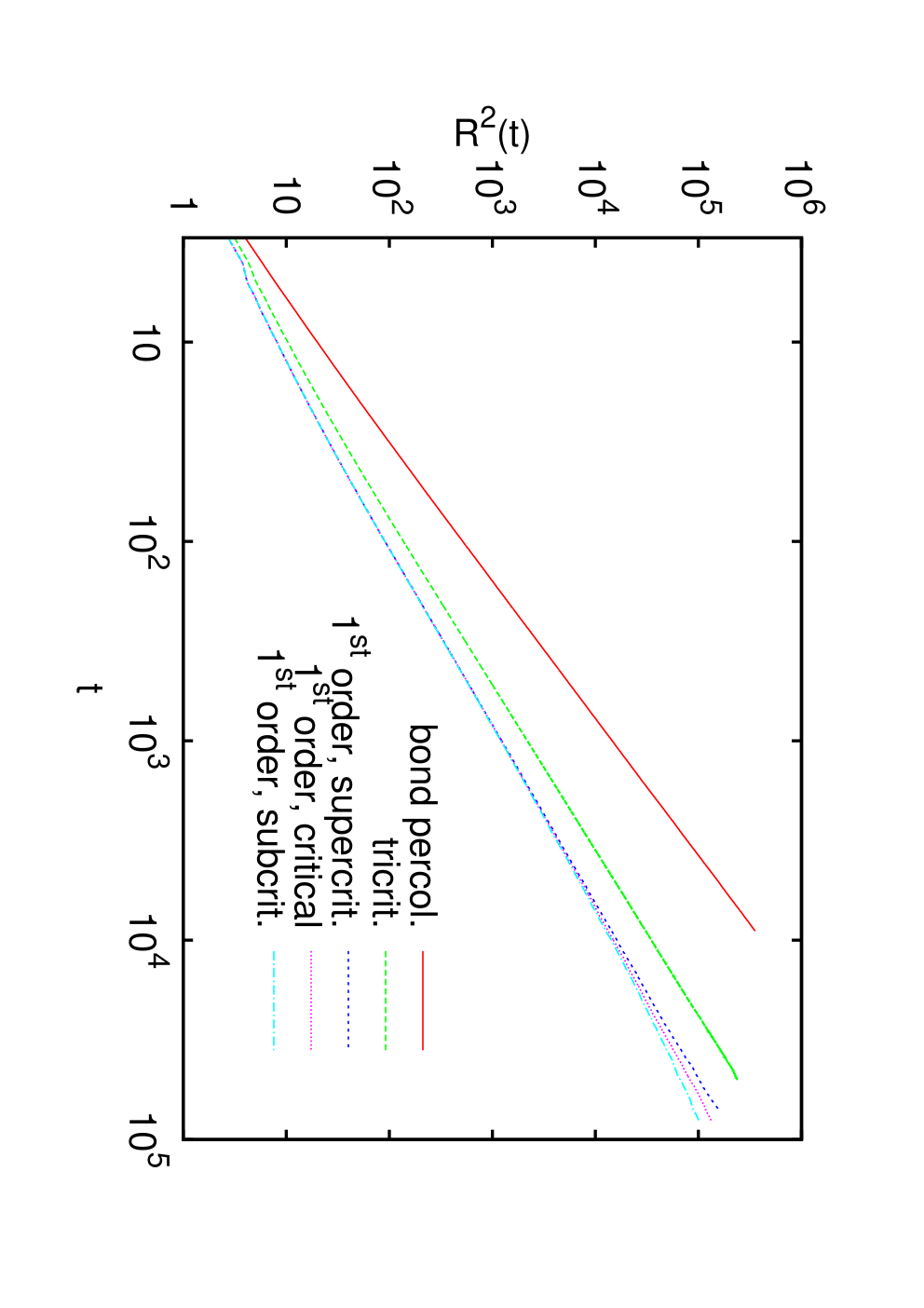
Further details will be given elsewhere [2]. They will concern statistics, the precise methods used to estimate exact tricritical properties, critical exponents for rough pinned surfaces, and the behavior in dimensions different from 3. Here we present just two more figures (Figs. 1 and 2), similar to Fig. 1 of the main text, that show the survival probability and the average squared radius of newly infected sites, measured from the starting point of the epidemic. They show pwer law behavior at the tricritical point (straight lines on log-log plots), with exponent values given in the main text.
A detailed comparison of our results with the field theoretic predictions of [3] will also be given in [2]. Here we just mention that our results for the critical exponents are qualitatively similar (the changes relative to the exponents for OP go in the right directions), but the agreement if far from perfect. The biggest disagreement is for , defined via . While a positive value,
| (1) |
with , was predicted in [3], we found .
II The epidemic threshold in the Dodds-Watts social contagion model
Since the original derivation of the result by Dodds and Watts [4] is somewhat cumbersome and involves more than a minimal set of assumptions, we give here a simpler derivation following the typical arguments for epidemic thresholds via consistency conditions [5, 6, 7]. We start by recalling the condition for the threshold of the standard epidemic process that leads to ordinary percolation, and we then modify a suitable reformulation so that it also applies to the more general case with different infection probabilities . We finally obtain the critical line and the tricritical point by straightforward algebra.
Let us call the probability that a node at one end of a randomly chosen link gets infected during an epidemic process on a sparse random network with degree distribution . If the infection can pass through any link with probability , then the locally treelike structure of the network results in the consistency condition [5, 6]
| (2) |
where . We write this as
| (3) |
(the subscripts stand for ‘ordinary percolation’). The percolation threshold is then defined by
| (4) |
where . Straightforward calculations give [8, 5, 6]
| (5) |
We also notice that .
In order to modify this to arbitrary infection probabilities for attacks following previous attacks, we first rewrite Eq. (3) such that contributions from different numbers of infected neighbors are separated. In order to do this we write , such that the first term is the probability that the considered node is not infected, while the second terms is the probability that it is infected, but it cannot infect its neighbor since the link cannot be passed. Similarly we write
| (6) |
such that each term in the sum corresponds to exactly infected neighbors. The modification to the generalized process is now obvious: We just have to replace the power by . Alternatively, we can replace it by where is the probability that attacks succeed in infecting the site. The formulations using and are fully equivalent.
Making this modification in Eq. (3) results in
| (7) | |||||
where GEP stands for ‘generalized epidemic process’. As before, the condition for criticality is
| (8) |
while the tricritical point is given by
| (9) |
Evaluating the derivatives is straightforward and gives [4]
| (10) |
and is given by Eq. (5). Notice that the location of the tricritical point does not depend on any with , and its existence does not put any constraints on them.
In the first order regime, the threshold condition for an epidemic is
| (11) |
which depends non-trivially both on the degree distribution and on all (or all ). For regular graphs with degree (i.e., ) and for all it approaches in the limit the linear relation . For , numerical solution of Eq. (11) gives the line plotted in Fig. 1 of the main text.
III The Strauss Model
We start from Eqs. (5) and (6) of Ref. [9], which read in our notation
| (12) |
and
| (13) |
Here is the link density and is defined in [9]. In the limit and of interest to us, these simplify to
| (14) |
and
| (15) |
Combining these gives an equation for in terms of and which we can write as
| (16) |

This equation can have four outcomes (see Fig. 3):
The critical point is thus obtained from , leading to the values quoted in the main text. The boundaries of the bistable region are given parametrically by
| (17) |
which give asymptotically for large
| (18) |
for the lower (upper) boundaries in a plot of versus (see Fig. 2 of [9]).
The actual transition curve , or rather , is obtained from a Maxwell construction: For some given value of , we first obtain as a function of from Eq. (16),
| (19) |
For any in the coexistence region, the equation has three roots . The transition point is then given by
| (20) |
For large , the curve of versus tends (except near the points and ) to a parabola, which gives in this limit as stated in the main text.
References
- [1] P. Grassberger, Comp. Phys. Commun. 147, 64 (2002)
- [2] P. Grassberger et al., to be published(2012)
- [3] H.-K. Janssen, M. Müller, and O. Stenull, Phys. Rev. E 70, 026114 (2004)
- [4] P. S. Dodds and D. J. Watts, Phys. Rev. Lett. 92, 218701 (2004)
- [5] M. E. J. Newman, S. H. Strogatz, and D. J. Watts, Phys. Rev. E 64, 026118 (2001)
- [6] M. E. J. Newman, Phys. Rev. Lett. 95, 108701 (2005)
- [7] S.-W. Son, G. Bizhani, C. Christensen, P. Grassberger, and M. Paczuski, Europhys. Lett. 97, 16006 (2012)
- [8] B. Bollobás, Random Graphs (Cambridge University Press, 1985)
- [9] J. Park and M. E. J. Newman, Phys. Rev. E 72, 026136 (2005)