跳到论文正文
W Papers独立论文阅读器 arXiv:1202.2912 论文正文 计算阅读时间 · 0%
引用这篇论文根据当前论文元数据生成,正式投稿前建议核对。


License: arXiv.org perpetual non-exclusive license
arXiv:1202.2912v1 [math.DG] 14 Feb 2012

On the structure of almost Einstein manifolds

Gang Tian Note: Partially supported by NSF grant DMS-0804095.    Bing Wang Note: Supported by NSF grant DMS-1006518 and funds from SCGP.
Abstract

In this paper, we study the structure of the limit space of a sequence of almost Einstein manifolds, which are generalizations of Einstein manifolds. Roughly speaking, such manifolds are the initial manifolds of some normalized Ricci flows whose scalar curvatures are almost constants over space-time in the L1L^{1}-sense, Ricci curvatures are bounded from below at the initial time. Under the non-collapsed condition, we show that the limit space of a sequence of almost Einstein manifolds has most properties which is known for the limit space of Einstein manifolds. As applications, we can apply our structure results to study the properties of Kähler manifolds.

1 Introduction

The regularity theory for non-collapsed Einstein manifolds has attracted many studies in last two decades, e.g., [3], [4], [37], [7], [8] etc. This theory and its extensions have played a crucial role in Kähle geometry, e.g., in constructing canonical metrics on Fano surfaces (c.f. [37], [15]).

Motivated by the study in Kähler geometry, in this paper, we prove new regularity results on the Gromov-Hausdorff limits of Riemannian manifolds with Ricci curvature bounded from below and which are weakly Einstein in an appropriate sense.

To be precise, we assume that (Xi,xi,gi)\left(X_{i},x_{i},g_{i}\right) is a sequence of non-collapsed Riemannian manifolds of dimension mm such that R​i​c≥−(m−1)Ric\geq-(m-1). The well-known Gromov compactness theorem states that by taking a subsequence if necessary, (Xi,xi,gi)\left(X_{i},x_{i},g_{i}\right) converges to a length space (X¯,x¯,g¯)\left(\bar{X},\bar{x},\bar{g}\right) in the Gromov-Hausdorff topology. A basic problem in the metric geometry concerns the regularity of the limit (X¯,x¯,g¯)\left(\bar{X},\bar{x},\bar{g}\right). Note that g¯\bar{g} is merely a length function in the Gromov compactness theorem. The fundamental work of Cheeger-Colding [7] shows initial and crucial structure properties for (X¯,x¯,g¯)\left(\bar{X},\bar{x},\bar{g}\right). In particular, it follows from [7] that tangent cones exist at every point y∈X¯y\in\bar{X}. Using these tangent cones, they gave a regular-singular decomposition of X¯\bar{X}. A point y∈X¯y\in\bar{X} is called regular or belongs to the regular part ℛ\mathcal{R} if every tangent cone at yy is isometric to the Euclidean space (ℝm,0,g𝔼)\left(\mathbb{R}^{m},0,g_{\mathbb{E}}\right). A point y∈Xy\in X is called singular or belongs to the singular part 𝒮\mathcal{S} if it is not regular, i.e., at yy, there exists some tangent cone (Y^,y^,g^)\left(\hat{Y},\hat{y},\hat{g}\right) which is not isometric to the Euclidean space. Clearly, we have X¯=ℛ∪𝒮\bar{X}=\mathcal{R}\cup\mathcal{S}. In general, it is unknown if ℛ\mathcal{R} is open and even if it is open, it may not be a manifold and g¯\bar{g} may not arise from a Riemannian metric in any classical senses. It is expected in general cases that ℛ\mathcal{R} has only locally Lipschitz structures at most. If gig_{i} has uniformly bounded Ricci curvature, then Cheeger-Colding proved that ℛ\mathcal{R} is an open manifold and 𝒮\mathcal{S} has Hausdorff codimension at least 22. Moreover, g¯\bar{g} is a C1,αC^{1,\alpha}-smooth metric. Furthermore, if (Xi,gi)(X_{i},g_{i}) is an Einstein manifold, then the convergence to X¯\bar{X} restricted to ℛ\mathcal{R} is actually in the C∞C^{\infty}-topology and g¯\bar{g} is a smooth Einstein metric in ℛ\mathcal{R} because of the regularity results from the PDE theory. However, in general, even if the convergence is weak, ℛ\mathcal{R} can still possibly be a smooth manifold. In this paper, we study when the limit can have smooth ℛ\mathcal{R} and g¯\bar{g} is an Einstein metric even if the convergence (Xi,xi,gi)→(X¯,x¯,g¯)\left(X_{i},x_{i},g_{i}\right)\to\left(\bar{X},\bar{x},\bar{g}\right) is only in the weak topology, say the Gromov-Hausdorff topology. Our study is analogous to the standard regularity problem in studying weak solutions for PDEs. In the case of the Einstein equation, because of its invariance under diffeomorphisms, there is not a good notion of weak solutions. Therefore, we first need to make clear what we mean by Einstein metrics in the weak sense. Now let us introduce the notion of almost Einstein manifolds we want to study.

Definitionin 1.

A sequence of closed Riemannian manifolds (Xim,xi,gi)\left(X_{i}^{m},x_{i},g_{i}\right) is called almost Einstein if the following conditions are satisfied.

  • •

    R​i​c​(gi)+gi≥0Ric(g_{i})+g_{i}\geq 0.

  • •

    xi∈Xix_{i}\in X_{i}, and |Bgi​(xi,1)|d​μgi≥κ|B_{g_{i}}(x_{i},1)|_{d\mu_{g_{i}}}\geq\kappa.

  • •

    The flow ∂∂t​g=−R​i​c+λi​g\displaystyle\frac{\partial{}}{\partial{t}}g\,=\,-Ric+\lambda_{i}g has a solution g⁡(t)g(t) with g⁡(0)=gig(0)=g_{i} on Xi×[0,1]X_{i}\times[0,1], where λi∈[−1,1]\lambda_{i}\in[-1,1] is a constant. Moreover, Ei=∫01∫Xi|R−m​λi|​𝑑μ​𝑑t→0E_{i}=\int_{0}^{1}\int_{X_{i}}|R-m\lambda_{i}|d\mu dt\to 0.

Note that the non-collapsed condition is included in our definition. This is because the condition ∫01∫Xi|R−m​λi|​d​μgi​𝑑t→0\int_{0}^{1}\int_{X_{i}}|R-m\lambda_{i}|d\mu_{g_{i}}dt\to 0 is not sufficient for proving the following results if collapsing occurs. However, we will not discuss this further in the current paper.

Clearly, if ∫01∫Xi|R−m​λi|​d​μgi​𝑑t≡0\int_{0}^{1}\int_{X_{i}}|R-m\lambda_{i}|d\mu_{g_{i}}dt\equiv 0, then this sequence is exactly a sequence of non-collapsed Einstein manifolds with bounded Einstein constants. Such a sequence was extensively studied in the literature. In fact, the condition ∫01∫Xi|R−m​λi|​d​μgi​𝑑t→0\int_{0}^{1}\int_{X_{i}}|R-m\lambda_{i}|d\mu_{g_{i}}dt\to 0 is crucial in establishing the regularity of ℛ\mathcal{R}. It turns out that almost Einstein limits have most known properties of Einstein limits. Our first theorem is as follows.

Theorem 1 (Structure theorem in Riemannian case).

Suppose (Xim,xi,gi)(X_{i}^{m},x_{i},g_{i}) is a sequence of almost Einstein manifolds. Let (X¯,x¯,g¯)\left(\bar{X},\bar{x},\bar{g}\right) be a Gromov-Hausdorff limit of (Xi,xi,gi)\left(X_{i},x_{i},g_{i}\right), λ¯\bar{\lambda} be the limit of λi\lambda_{i}.

Then the limit space (X¯,x¯,g¯)\left(\bar{X},\bar{x},\bar{g}\right) is a metric space with disjoint decomposition X¯=ℛ∪𝒮\bar{X}=\mathcal{R}\cup\mathcal{S}, where ℛ\mathcal{R} is the regular part of X¯\bar{X}, 𝒮\mathcal{S} is the singular part of X¯\bar{X}. They satisfy the following properties.

  • •

    (ℛ,g¯)\left(\mathcal{R},\bar{g}\right) is a smooth, convex, open Riemannian manifold.

  • •

    R​i​c​(g¯)+λ¯​g¯=0\displaystyle Ric(\bar{g})+\bar{\lambda}\bar{g}=0.

  • •

    If 0<p<10<p<1 and ρ≥1\rho\geq 1, then ∫ℛ∩B⁡(x¯,ρ)|R​m|p​𝑑μ<C⁡(m,κ,p,ρ)\int_{\mathcal{R}\cap B(\bar{x},\rho)}|Rm|^{p}d\mu<C(m,\kappa,p,\rho).

  • •

    If y∈𝒮y\in\mathcal{S}, (X^,y^,g^)\left(\hat{X},\hat{y},\hat{g}\right) is a tangent space of X¯\bar{X} at the point yy, then

    dG​H​((Bg^​(y^,1),g^),(B⁡(0,1),g𝔼))>ϵ¯​(m),\displaystyle d_{GH}\left(\left(B_{\hat{g}}(\hat{y},1),\hat{g}\right),\left(B(0,1),g_{\mathbb{E}}\right)\right)>\bar{\epsilon}(m),

    where B⁡(0,1)B(0,1) is the standard unit ball in ℝm\mathbb{R}^{m}.

  • •

    dimℋ𝒮≤m−2\dim_{\mathcal{H}}\mathcal{S}\leq m-2.

Note that the convexity of ℛ\mathcal{R} and the integral bound of |R​m||Rm| follow directly from the work of [29] and [11] respectively. We list these results here just for completeness of the known results of Einstein limit.

We observe that if (Mi,xi,gi)(M_{i},x_{i},g_{i}) is a sequence of Kähler manifolds, then by a result of the first author and Z. Zhang (c.f. [40]), the Ricci flow ∂∂t​g=−R​i​c+λi​g\displaystyle\frac{\partial{}}{\partial{t}}g\,=\,-Ric+\lambda_{i}g has a solution with g⁡(0)=gig(0)=g_{i} on Mi×[0,1]M_{i}\times[0,1] so long as λi​[ωi]+(eλi​t−1)​c1​(Mi)>0\lambda_{i}[\omega_{i}]+\left(e^{\lambda_{i}t}-1\right)c_{1}(M_{i})>0, where ωi\omega_{i} denotes the Kähler form of gig_{i}. Moreover, if R−n​λi≥0R-n\lambda_{i}\geq 0 and its average tends to zero as ii goes to infinity, then one can show that EiE_{i} tends to zero. Thus, the third condition of Definition 1 is essentially automatic if R−n​λi≥0R-n\lambda_{i}\geq 0 and its average tends to zero. This shows that the Kähler case is better behaved. A natural question is whether or not the same holds for general Riemannian metrics with Ricci curvature bounded from below. More precisely, can one solve the above Ricci flow with initial value g0g_{0} in [0,a][0,a] such that aa depends only on the lower bound of Ricci curvature of g0g_{0}?

The following theorem strengthens Theorem 1 for Kähler manifolds. We say that a sequence of closed Kähler manifolds (Min,xi,gi,Ji)\left(M_{i}^{n},x_{i},g_{i},J_{i}\right) is almost Kähler-Einstein if it is almost Einstein of dimension m=2​nm=2n and satisfies Fi=∫Mi|R​i​c−λi​gi|​d​μgi→0F_{i}=\int_{M_{i}}|Ric-\lambda_{i}g_{i}|d\mu_{g_{i}}\to 0.

Theorem 2 (Structure theorem in Kähler case).

Suppose (Min,xi,gi,Ji)(M_{i}^{n},x_{i},g_{i},J_{i}) is a sequence of almost Kähler Einstein manifolds. Let (M¯,x¯,g¯)\left(\bar{M},\bar{x},\bar{g}\right) be a Gromov-Hausdorff limit of (Mi,xi,gi)\left(M_{i},x_{i},g_{i}\right), λ¯\bar{\lambda} be the limit of λi\lambda_{i}.

Then the limit space (M¯,x¯,g¯)\left(\bar{M},\bar{x},\bar{g}\right) is a metric space with the regular-singular disjoint decomposition M¯=ℛ∪𝒮\bar{M}=\mathcal{R}\cup\mathcal{S}. They satisfy the following properties.

  • •

    There exists a complex structure J¯\bar{J} on ℛ\mathcal{R} such that (ℛ,g¯,J¯)\left(\mathcal{R},\bar{g},\bar{J}\right) is a smooth, convex, open Kähler manifold.

  • •

    R​i​c​(g¯)+λ¯​g¯=0\displaystyle Ric(\bar{g})+\bar{\lambda}\bar{g}=0.

  • •

    If 0<p<20<p<2 and ρ≥1\rho\geq 1, then ∫ℛ∩B⁡(x¯,ρ)|R​m|p​𝑑μ<C⁡(n,κ,p,ρ)\int_{\mathcal{R}\cap B(\bar{x},\rho)}|Rm|^{p}d\mu<C(n,\kappa,p,\rho).

  • •

    If y∈𝒮y\in\mathcal{S}, (M^,y^,g^)\left(\hat{M},\hat{y},\hat{g}\right) is a tangent space of M¯\bar{M} at the point yy, then

    dG​H​((Bg^​(y^,1),g^),(B⁡(0,1),g𝔼))>ϵ¯​(2​n),\displaystyle d_{GH}\left(\left(B_{\hat{g}}(\hat{y},1),\hat{g}\right),\left(B(0,1),g_{\mathbb{E}}\right)\right)>\bar{\epsilon}(2n),

    where B⁡(0,1)B(0,1) is the standard unit ball in ℝ2​n\mathbb{R}^{2n}.

  • •

    dimℋ𝒮≤2​n−4\dim_{\mathcal{H}}\mathcal{S}\leq 2n-4.

Our proof of the above theorems is based on the works of [7], [8], [30] et al. We need to establish two new technical results. The first one is a pseudo-locality result (Theorem 3.1) which is similar to Theorem 10.1 and 10.3 of [30]. Basically, we need to bound curvature along the Ricci flow whenever the initial metric has its Ricci curvature bounded from below and the volume ratios of its geodesic balls are sufficiently close to the Euclidean one. Our proof for this pseudo-locality uses an argument due to Perelman. The second one is a delicate bound of the Gromov-Hausdorff distance between metrics along the Ricci flow (c.f. Theorem 4.2). This bound plays a role similar to the gap theorem for Einstein limits and is crucial for us to finish the proof of Theorem 1 and Theorem 2.

The organization of this paper is as follows. In Section 2, we discuss some standard estimates which will be repeatedly used in the whole paper. In Section 3, we prove a new pseudo-locality result, i.e., Theorem 3.1. Using this new pseudo-locality, we prove a gap theorem (Theorem 4.2) in Section 4. Then in section 5, we use pseudo-locality theorem, gap theorem and the fact that scalar curvature is almost constant to show the structure theorems in both Riemannian and Kähler cases. Finally, we construct examples of almost Kähler Einstein manifolds and discuss the applications of our structure theorems to Kähler geometry.

Acknowledgment The second named author is very grateful to professor Xiuxiong Chen and professor Simon Donaldson for their constant support. He appreciate SCGP (Simons Center for Geometry and Physics) for offering him the wonderful working condition. Part of this work was done when the second named author was visiting BICMR (Beijing International Center of Mathematical Research) during the summer of 2011, he would like to thank BICMR for its hospitality.

2 Elementary estimates

Before we go to discussion in details, let’s fix some notations first. We assume XX to be a closed Riemannian manifold of dimension m≥3m\geq 3, MM to be a closed Kähler manifold of complex dimension n≥2n\geq 2, real dimension m=2​n≥4m=2n\geq 4. We denote the volume of standard unit ball in ℝm\mathbb{R}^{m} by ωm\omega_{m}. We say A<<BA<<B for two positive quantities AA and BB if there is a universal small constant c=c⁡(m)c=c(m) such that A<c​BA<cB. If not mentioned in particular, the constant CC may be different from line to line.

In this paper, we often assume {(X,g(t)),0≤t≤1}\left\{(X,g(t)),0\leq t\leq 1\right\} satisfies the evolution equation

∂∂t​g=−R​i​c+λ0​g\displaystyle\frac{\partial{}}{\partial{t}}g=-Ric+\lambda_{0}g (1)

for some constant λ0\lambda_{0} with |λ0|≤1|\lambda_{0}|\leq 1. Note that this flow may not preserve the volume. However, by abuse of notation, we also call (1) as a normalized Ricci flow solution. Define

g~​(s)≜{(1−2​λ0​s)​g​(log⁡(1−2​λ0​s)−λ0),if​λ0≠0;g⁡(2​s),if​λ0=0.\displaystyle\tilde{g}(s)\triangleq\begin{cases}&\left(1-2\lambda_{0}s\right)g\left(\frac{\log(1-2\lambda_{0}s)}{-\lambda_{0}}\right),\;\textrm{if}\;\lambda_{0}\neq 0;\\ &g(2s),\;\textrm{if}\;\lambda_{0}=0.\end{cases} (2)

Then ∂∂s​g~=−2​R​i​c​(g~)\displaystyle\frac{\partial{}}{\partial{s}}\tilde{g}=-2Ric(\tilde{g}), which is the (unnormalized) Ricci flow equation. Clearly, g~​(0)=g​(0)\tilde{g}(0)=g(0). For simplicity of notation, define hi​j≜Ri​j−λ0​gi​jh_{ij}\triangleq R_{ij}-\lambda_{0}g_{ij}, H≜R−m​λ0H\triangleq R-m\lambda_{0}. Simple calculation yields

∂∂t​hi​j=12​Δ​hi​j+Rp​i​j​q​hi​j−hi​p​hp​j,\displaystyle\frac{\partial{}}{\partial{t}}h_{ij}=\frac{1}{2}\Delta h_{ij}+R_{pijq}h_{ij}-h_{ip}h_{pj}, (3)

which implies

∂∂t​|h|≤12​Δ​|h|+|R​m|​|h|.\displaystyle\frac{\partial{}}{\partial{t}}|h|\leq\frac{1}{2}\Delta|h|+|Rm||h|. (4)

Take trace of (3), we obtain

∂∂t​H=12​Δ​H+|h|2+λ0​H.\displaystyle\frac{\partial{}}{\partial{t}}H=\frac{1}{2}\Delta H+|h|^{2}+\lambda_{0}H. (5)

Define Hm​i​n​(t)≜minx∈X⁡H⁡(x,t)\displaystyle H_{min}(t)\triangleq\min_{x\in X}H(x,t). Apply maximum principle to (5), we obtain

∂∂t​Hm​i​n​(t)≥λ0​Hm​i​n​(t)⇒Hm​i​n​(t)≥eλ0​t​Hm​i​n​(0).\displaystyle\frac{\partial{}}{\partial{t}}H_{min}(t)\geq\lambda_{0}H_{min}(t)\Rightarrow H_{min}(t)\geq e^{\lambda_{0}t}H_{min}(0). (6)

In particular, the condition H≥0H\geq 0 is preserved by the normalized Ricci flow (1).

It follows from (1) that the distance derivative with respect to time is controlled by the |R​i​c−λ0​g||Ric-\lambda_{0}g| along the shortest geodesic. However, a more delicate analysis shows that the lower bound of the distance derivative depends only on the local Ricci upper bound around the end points.

Proposition 2.1 (c.f. section 17 of [25], or Lemma 8.3(b) of [30]).

Suppose {(X,g(t)),0≤t≤1}\left\{(X,g(t)),0\leq t\leq 1\right\} is a normalized Ricci flow solution ∂∂t​g=−R​i​c+λ0​g\frac{\partial{}}{\partial{t}}g=-Ric+\lambda_{0}g with |λ0|≤1|\lambda_{0}|\leq 1. Suppose 0≤t0≤10\leq t_{0}\leq 1, x1,x2x_{1},x_{2} are two points in XX such that R​i​c​(x,t0)≤(m−1)​KRic(x,t_{0})\leq(m-1)K when dg⁡(t0)​(x,x1)<r0d_{g(t_{0})}(x,x_{1})<r_{0} or dg⁡(t0)​(x,x2)<r0d_{g(t_{0})}(x,x_{2})<r_{0}. Then

dd​t​dg⁡(t)​(x1,x2)|t=t0≥12​λ0​dg⁡(t0)​(x1,x2)−(m−1)​(23​K​r0+r0−1).\displaystyle\left.\frac{d}{dt}d_{g(t)}(x_{1},x_{2})\right|_{t=t_{0}}\geq\frac{1}{2}\lambda_{0}d_{g(t_{0})}(x_{1},x_{2})-(m-1)\left(\frac{2}{3}Kr_{0}+r_{0}^{-1}\right). (7)
Proof.

Without loss of generality, one can assume t0=0t_{0}=0. Then the proof is just an application of the renormalization equation (2) and Lemma 8.3(b) of [30]. ∎

Suppose Ω\Omega is a compact manifold with boundary. The following lemmas are standard (c.f. [27]).

Lemma 2.1.

Suppose (X,g)(X,g) is a complete manifold, x0∈Xx_{0}\in X, 0<r≤10<r\leq 1. Suppose r−m​|B⁡(x0,r)|≥κr^{-m}|B(x_{0},r)|\geq\kappa and r2​R​i​c≥−(m−1)r^{2}Ric\geq-(m-1) in B⁡(x0,2​r)B(x_{0},2r). Let Ω=B⁡(x0,r)\Omega=B(x_{0},r). Then the following properties are satisfied.

  • •

    The isoperimetric constant of Ω\Omega is uniformly bounded by CI=CI​(m,κ)C_{I}=C_{I}(m,\kappa).

  • •

    The Sobolev constant of Ω\Omega is uniformly bounded by CS=CS​(m,κ)C_{S}=C_{S}(m,\kappa).

  • •

    The Neuman Poincaré constant of Ω\Omega is uniformly bounded by CP=CP​(m,κ)C_{P}=C_{P}(m,\kappa).

Lemma 2.2.

Suppose (X,g)(X,g) is a complete Riemannian manifold, x0∈Xx_{0}\in X. Suppose the following conditions are satisfied.

  • •

    For every 0<r<20<r<2, we have CV−1<|B⁡(x0,r)|​r−m<CVC_{V}^{-1}<|B(x_{0},r)|r^{-m}<C_{V}.

  • •

    The Sobolev constant of B⁡(x0,2)B(x_{0},2) is bounded by CSC_{S}.

  • •

    The Poincaré constant of B⁡(x0,2)B(x_{0},2) is bounded by CPC_{P}.

  • •

    |a|+|ψ|<CF|a|+|\psi|<C_{F} on B⁡(x0,2)B(x_{0},2).

Suppose φ≥0\varphi\geq 0 satisfies the inequality (−Δ+a)​φ≥ψ\left(-\Delta+a\right)\varphi\geq\psi in the distribution sense, then

∫B⁡(x0,1)φ≤C⁡(1+infB⁡(x0,12)φ),\displaystyle\int_{B(x_{0},1)}\varphi\leq C\left(1+\inf_{B\left(x_{0},\frac{1}{2}\right)}\varphi\right), (8)

where C=C⁡(m,CV,CS,CP,CF)C=C(m,C_{V},C_{S},C_{P},C_{F}). Consequently, for every 0<ρ<10<\rho<1, we have

ρ−m​∫B⁡(x0,ρ)φ≤C⁡(ρ2+infB⁡(x0,ρ2)φ),\displaystyle\rho^{-m}\int_{B(x_{0},\rho)}\varphi\leq C\left(\rho^{2}+\inf_{B\left(x_{0},\frac{\rho}{2}\right)}\varphi\right), (9)

where CC is the same constant as in (8).

Proof.

Let φ¯=φ+CF\bar{\varphi}=\varphi+C_{F}. We compute

(−Δ+a)​φ¯≥ψ+a​CF=CF​(a+CF−1​ψ)≥−CF​|a+CF−1​ψ|≥−|a+CF−1​ψ|​φ¯≥−(|a|+1)​φ¯.\displaystyle\left(-\Delta+a\right)\bar{\varphi}\geq\psi+aC_{F}=C_{F}\left(a+C_{F}^{-1}\psi\right)\geq-C_{F}\left|a+C_{F}^{-1}\psi\right|\geq-\left|a+C_{F}^{-1}\psi\right|\bar{\varphi}\geq-\left(|a|+1\right)\bar{\varphi}.

It follows

Δ​φ¯≤(2​|a|+1)​φ¯≤(2​CF+1)​φ¯.\Delta\bar{\varphi}\leq\left(2|a|+1\right)\bar{\varphi}\leq\left(2C_{F}+1\right)\bar{\varphi}.

By the standard De Giorgi-Nash-Moser iteration (c.f. Lemma 11.2 of [27]), we have

∫B⁡(x0,1)φ¯≤C​infB⁡(x0,12)φ¯\displaystyle\int_{B(x_{0},1)}\bar{\varphi}\leq C\inf_{B\left(x_{0},\frac{1}{2}\right)}\bar{\varphi}

for some CC depending on m,CV,CS,CPm,C_{V},C_{S},C_{P} and CFC_{F}. This in turn implies (8).

Fix 0<ρ<10<\rho<1. Let g~=ρ−2​g\tilde{g}=\rho^{-2}g. By the scaling property of the Laplacian operator, we see that

(−Δ+a)​φ≥ψ⇔−ρ−2​Δg~​φ+a​φ≥ψ⇔−Δg~​(ρ−2​φ)+ρ2​a​(ρ−2​φ)≥ψ.\displaystyle\left(-\Delta+a\right)\varphi\geq\psi\Leftrightarrow-\rho^{-2}\Delta_{\tilde{g}}\varphi+a\varphi\geq\psi\Leftrightarrow-\Delta_{\tilde{g}}\left(\rho^{-2}\varphi\right)+\rho^{2}a\left(\rho^{-2}\varphi\right)\geq\psi.

Let φ~=ρ−2​φ\tilde{\varphi}=\rho^{-2}\varphi, we have

−Δg~​φ~+ρ2​a​φ~≥ψ.\displaystyle-\Delta_{\tilde{g}}\tilde{\varphi}+\rho^{2}a\tilde{\varphi}\geq\psi.

Consider this system under the metric g~\tilde{g}. The four estimates hold for this new system, so we obtain

∫Bg~​(x0,1)φ~≤C⁡(1+infBg~​(x0,12)φ~),\displaystyle\int_{B_{\tilde{g}}(x_{0},1)}\tilde{\varphi}\leq C\left(1+\inf_{B_{\tilde{g}}\left(x_{0},\frac{1}{2}\right)}\tilde{\varphi}\right),

which is the same as (9) since φ~=ρ−2​φ\tilde{\varphi}=\rho^{-2}\varphi. ∎

Combing Lemma 2.1 and Lemma 2.2, we obtain the following Proposition, which is very useful in the study of boundary estimate.

Proposition 2.2.

Suppose (X,x0,g)(X,x_{0},g) is a complete Riemannian manifold. Suppose 0<r≤10<r\leq 1, r−m​|B⁡(x0,r)|≥κr^{-m}|B(x_{0},r)|\geq\kappa, r2​R​i​c≥−(m−1)r^{2}Ric\geq-(m-1) on B⁡(x0,2​r)B(x_{0},2r). Suppose φ≥0\varphi\geq 0 satisfies the inequality (−Δ+a)​φ≥ψ\left(-\Delta+a\right)\varphi\geq\psi for |a|+|ψ|<CF|a|+|\psi|<C_{F}. Then for every 0<ρ≤r0<\rho\leq r, we have

ρ−m​∫B⁡(x0,ρ)φ≤C⁡(ρ2+infB⁡(x0,ρ2)φ),\displaystyle\rho^{-m}\int_{B(x_{0},\rho)}\varphi\leq C\left(\rho^{2}+\inf_{B\left(x_{0},\frac{\rho}{2}\right)}\varphi\right), (10)

for some constant C=C⁡(m,κ,CF)C=C(m,\kappa,C_{F}).

3 A pseudo-locality theorem

Under the Ricci flow, an “almost-Euclidean” region cannot become singular suddenly. This is the principle of pseudo-locality as stated by Perelman in section 10 of [30]. Perelman developed some pseudo-locality theorems by regarding “almost” as close of isoperimetric constant and scalar lower bound. Of course, this is not the unique “almost-Euclidean” condition. In this section, we will develop similar pseudo-locality properties by explaining “almost-Euclidean” balls as balls whose volume ratio and Ricci lower bound is close to that of the Euclidean balls’.

Proposition 3.1 (A pseudo-locality property, compare Theorem 10.1 and Theorem 10.3 of Perelman [30]).

For every 0<α<1100​m0<\alpha<\frac{1}{100m}, there exist constants δ=δ⁡(m,α),ϵ=ϵ⁡(m,α)\delta=\delta(m,\alpha),\epsilon=\epsilon(m,\alpha) with the following properties.

Suppose {(X,g(t)),0≤t≤1}\left\{(X,g(t)),0\leq t\leq 1\right\} is a Ricci flow solution, x0∈Xx_{0}\in X. Suppose

R​i​c​(x,0)≥−(m−1)​δ4,∀x∈Bg⁡(0)​(x0,δ−1).\displaystyle Ric(x,0)\geq-(m-1)\delta^{4},\quad\forall\;x\in B_{g(0)}\left(x_{0},\delta^{-1}\right). (11)
δm​|Bg⁡(0)​(x0,δ−1)|d​μg⁡(0)≥(1−δ)​ωm.\displaystyle\delta^{m}\left|B_{g(0)}\left(x_{0},\delta^{-1}\right)\right|_{d\mu_{g(0)}}\geq(1-\delta)\omega_{m}. (12)

Then we have

|Bg⁡(t)​(x,t)|d​μg⁡(t)≥κ′​tm2,\displaystyle\left|B_{g(t)}\left(x,\sqrt{t}\right)\right|_{d\mu_{g(t)}}\geq\kappa^{\prime}t^{\frac{m}{2}}, (13)
|R​m|​(x,t)≤α​t−1+ϵ−2,∀x∈Bg⁡(0)​(x0,ϵ),t∈(0,ϵ2],\displaystyle|Rm|(x,t)\leq\alpha t^{-1}+\epsilon^{-2},\quad\forall\;x\in B_{g(0)}\left(x_{0},\epsilon\right),\;t\in(0,\epsilon^{2}], (14)

where κ′=κ′​(m)\kappa^{\prime}=\kappa^{\prime}(m) is a universal constant.

Proof.

We only prove (14). The proof of (13) follows verbatim.

If the statement was false, we can find a sequence of δk,ϵk→0\delta_{k},\epsilon_{k}\to 0, xk∈Xkx_{k}\in X_{k} such that (11) and (12) hold. However, (14) are violated.

Following the proof of Perelman’s pseudo-locality theorem, we can find a sequence of functions uku_{k} which are compactly supported on B⁡(xk,1)B(x_{k},1) and satisfy (See the end of the proof of Theorem 10.1 of [30]):

∫B⁡(xk,1)uk=1,\displaystyle\int_{B(x_{k},1)}u_{k}=1, (15)
∫B⁡(xk,1){12​|∇fk|2+fk−m}​uk≤−η<0,\displaystyle\int_{B(x_{k},1)}\left\{\frac{1}{2}\left|\nabla f_{k}\right|^{2}+f_{k}-m\right\}u_{k}\leq-\eta<0, (16)

where uk=(2​π)−m2​e−fku_{k}=(2\pi)^{-\frac{m}{2}}e^{-f_{k}}. Of course, here we regard d​μgk​(0)d\mu_{g_{k}(0)} as the default measure. Let u¯k=uk\bar{u}_{k}=\sqrt{u_{k}}. These equations can be written as

∫B⁡(xk,1)u¯k2=1,\displaystyle\int_{B(x_{k},1)}\bar{u}_{k}^{2}=1,
∫B⁡(xk,1){2​|∇u¯k|2−2​u¯k2​log⁡u¯k−m⁡(1+log⁡2​π)​u¯k2}≤−η.\displaystyle\int_{B(x_{k},1)}\left\{2|\nabla\bar{u}_{k}|^{2}-2\bar{u}_{k}^{2}\log\bar{u}_{k}-m\left(1+\log\sqrt{2\pi}\right)\bar{u}_{k}^{2}\right\}\leq-\eta.

Denote by ℱk​(uk)\mathcal{F}_{k}(u_{k}) the integral

∫B⁡(xk,1){2​|∇u¯k|2−2​u¯k2​log⁡u¯k−m⁡(1+log⁡2​π)​u¯k2}.\int_{B(x_{k},1)}\left\{2|\nabla\bar{u}_{k}|^{2}-2\bar{u}_{k}^{2}\log\bar{u}_{k}-m\left(1+\log\sqrt{2\pi}\right)\bar{u}_{k}^{2}\right\}.

Clearly, ℱk\mathcal{F}_{k} is a functional on the space of functions u¯∈W01,2​(B⁡(xk,1))\bar{u}\in W_{0}^{1,2}(B(x_{k},1)) satisfying ∫B⁡(xk,1)u¯2=1\int_{B(x_{k},1)}\bar{u}^{2}=1. By the result of Rothaus ([33]), we see that ℱk\mathcal{F}_{k} has a minimizer φk\varphi_{k}, which satisfies the Euler-Lagrange equation

−2​Δ​φk−2​φk​log⁡φk−m⁡(1+log⁡2​π)​φk=λk​φk.\displaystyle-2\Delta\varphi_{k}-2\varphi_{k}\log\varphi_{k}-m\left(1+\log\sqrt{2\pi}\right)\varphi_{k}=\lambda_{k}\varphi_{k}. (17)

On one hand, by the choice of λk\lambda_{k}, we have

λk=ℱ⁡(φk)≤ℱ⁡(u¯k)≤−η<0.\displaystyle\lambda_{k}=\mathcal{F}(\varphi_{k})\leq\mathcal{F}(\bar{u}_{k})\leq-\eta<0.

On the other hand, integrating (17) over B⁡(xk,1)B(x_{k},1) implies

λk+m⁡(1+log⁡2​π)\displaystyle\quad\lambda_{k}+m\left(1+\log\sqrt{2\pi}\right)
=∫2​|∇φk|2−2​∫φk2​log⁡φk\displaystyle=\int 2|\nabla\varphi_{k}|^{2}-2\int\varphi_{k}^{2}\log\varphi_{k}
≥∫2​|∇φk|2−2​∫φk2⋅(m2​e​φk2m)\displaystyle\geq\int 2|\nabla\varphi_{k}|^{2}-2\int\varphi_{k}^{2}\cdot\left(\frac{m}{2e}\varphi_{k}^{\frac{2}{m}}\right)
=∫2​|∇φk|2−me​∫φk⋅φkm+2m.\displaystyle=\int 2|\nabla\varphi_{k}|^{2}-\frac{m}{e}\int\varphi_{k}\cdot\varphi_{k}^{\frac{m+2}{m}}. (18)

In the third step, we used the fact log⁡x≤m2​e​x2m\log x\leq\frac{m}{2e}x^{\frac{2}{m}} for every positive xx. Plug Hölder inequality into (18) yields

λk+m⁡(1+log⁡2​π)\displaystyle\quad\lambda_{k}+m\left(1+\log\sqrt{2\pi}\right)
≥∫2​|∇φk|2−me​(∫φk2​mm−2)m−22​m⋅(∫φk2)m+22​m\displaystyle\geq\int 2|\nabla\varphi_{k}|^{2}-\frac{m}{e}\left(\int\varphi_{k}^{\frac{2m}{m-2}}\right)^{\frac{m-2}{2m}}\cdot\left(\int\varphi_{k}^{2}\right)^{\frac{m+2}{2m}}
=∫2​|∇φk|2−2⋅m2​e​(∫φk2​mm−2)m−22​m\displaystyle=\int 2|\nabla\varphi_{k}|^{2}-2\cdot\frac{m}{2e}\left(\int\varphi_{k}^{\frac{2m}{m-2}}\right)^{\frac{m-2}{2m}}
≥∫2​|∇φk|2−{a2​(∫φk2​mm−2)m−2m+m24​a2​e2},\displaystyle\geq\int 2|\nabla\varphi_{k}|^{2}-\left\{a^{2}\left(\int\varphi_{k}^{\frac{2m}{m-2}}\right)^{\frac{m-2}{m}}+\frac{m^{2}}{4a^{2}e^{2}}\right\}, (19)

where aa is a positive constant to be determined. Apply Lemma 2.1, we obtain uniform bound for the Sobolev constant of B⁡(xk,1)B(x_{k},1). It follows that

(∫B⁡(xk,1)φk2​mm−2)m−2m≤CS​∫B⁡(xk,1)(φk2+|∇φk|2).\displaystyle\left(\int_{B(x_{k},1)}\varphi_{k}^{\frac{2m}{m-2}}\right)^{\frac{m-2}{m}}\leq C_{S}\int_{B(x_{k},1)}\left(\varphi_{k}^{2}+|\nabla\varphi_{k}|^{2}\right). (20)

Let a2=2CSa^{2}=\frac{2}{C_{S}} and put (20) into (19), we obtain

λk+m⁡(1+log⁡2​π)≥(2−a2​CS)​∫|∇φk|2−(a2​CS+m24​a2​e2)=−(2+m2​CS8​e2).\displaystyle\lambda_{k}+m\left(1+\log\sqrt{2\pi}\right)\geq(2-a^{2}C_{S})\int|\nabla\varphi_{k}|^{2}-\left(a^{2}C_{S}+\frac{m^{2}}{4a^{2}e^{2}}\right)=-\left(2+\frac{m^{2}C_{S}}{8e^{2}}\right). (21)

Recall that λk≤−η<0\lambda_{k}\leq-\eta<0, from (21) we see that there exists a constant CλC_{\lambda}, which depends on m,CSm,C_{S}, such that

|λk|<Cλ.\displaystyle|\lambda_{k}|<C_{\lambda}. (22)

Note that the Euler-Lagrangian equation of φk\varphi_{k} can be written as

−Δ​φk=(12​(m+m​log⁡2​π+λk)+log⁡φk)​φk.\displaystyle-\Delta\varphi_{k}=\left(\frac{1}{2}\left(m+m\log\sqrt{2\pi}+\lambda_{k}\right)+\log\varphi_{k}\right)\varphi_{k}. (23)

Define φ¯k≜max⁡{φk,1}\bar{\varphi}_{k}\triangleq\max\left\{\varphi_{k},1\right\}. Since log⁡x≤m2​e​x2m\log x\leq\frac{m}{2e}x^{\frac{2}{m}} for every x>0x>0, it follows from (23) that φ¯k\bar{\varphi}_{k} satisfies the inequality

−Δ​φ¯k≤12​(m+m​log⁡2​π+λk+me​φ¯k2m)​φ¯k\displaystyle-\Delta\bar{\varphi}_{k}\leq\frac{1}{2}\left(m+m\log\sqrt{2\pi}+\lambda_{k}+\frac{m}{e}\bar{\varphi}_{k}^{\frac{2}{m}}\right)\bar{\varphi}_{k} (24)

in the distribution sense. Clearly, we can uniformly bound the Lm​(B⁡(xk,2))L^{m}(B(x_{k},2))-norm of

12​(m+m​log⁡2​π+λk+me​φ¯k2m),\displaystyle\frac{1}{2}\left(m+m\log\sqrt{2\pi}+\lambda_{k}+\frac{m}{e}\bar{\varphi}_{k}^{\frac{2}{m}}\right),

where m>m2m>\frac{m}{2}. Note that B⁡(xk,2)B(x_{k},2) has a uniform Sobolev constant CSC_{S}. Then the standard Moser iteration implies that

‖φ¯k‖C0​(B⁡(xk,1))≤C​‖φ¯k‖L2​(B⁡(xk,2))≤C,\displaystyle{\|\bar{\varphi}_{k}\|}_{C^{0}(B(x_{k},1))}\leq C{\|\bar{\varphi}_{k}\|}_{L^{2}(B(x_{k},2))}\leq C,

which in turn implies

‖φk‖C0​(B⁡(xk,1))≤C1=C1​(m,CS,Cλ).\displaystyle{\|\varphi_{k}\|}_{C^{0}(B(x_{k},1))}\leq C_{1}=C_{1}(m,C_{S},C_{\lambda}). (25)

Recall that Ricci curvature is uniformly bounded from below on B⁡(xk,2)B(x_{k},2), the estimate of Cheng-Yau (c.f. [16], section 6 of [27]) implies that

|∇φk​(x)|≤C2​(m,d⁡(x,∂B⁡(xk,1))),∀x∈B⁡(xk,1).\displaystyle|\nabla\varphi_{k}(x)|\leq C_{2}(m,d(x,\partial B(x_{k},1))),\quad\forall x\in B(x_{k},1). (26)

In view of the non-collapsed condition and Ricci lower bound, we have the convergence in the pointed Gromov-Hausdorff topology,

(Xk,xk,gk(0))→G​r​o​m​o​v−H​a​u​s​d​o​r​f​f(X∞,x∞,g∞).\displaystyle\left(X_{k},x_{k},g_{k}(0)\right){\mathrel{\to}^{Gromov-Hausdorff}}\left(X_{\infty},x_{\infty},g_{\infty}\right). (27)

Combining (25), (26) and (27), we obtain a locally-Lipschitz limit function φ∞\varphi_{\infty} on B⁡(x∞,1)⊂X∞B(x_{\infty},1)\subset X_{\infty} with ‖φ∞‖C0​(B⁡(x∞,1))≤C1\displaystyle{\|\varphi_{\infty}\|}_{C^{0}(B(x_{\infty},1))}\leq C_{1}. In general, it is hard to expect φ∞\varphi_{\infty} to be better than a locally-Lipschitz function. However, by Theorem 0.8 of [18], we know that X∞X_{\infty} is isometric to the Euclidean space (ℝm,g𝔼)\left(\mathbb{R}^{m},g_{\mathbb{E}}\right), which has a lot of excellent properties. We will use these properties to show that φ∞\varphi_{\infty} has much better regularity than a general locally Lipshitz function.

Claim 1.

φ∞\varphi_{\infty} can be extended to be a continuous function defined on B⁡(x∞,1)¯\overline{B(x_{\infty},1)} with

φ∞|∂B⁡(x∞,1)=0.\displaystyle\varphi_{\infty}|_{\partial B(x_{\infty},1)}=0. (28)

It suffices to show limr→0‖φ∞‖L∞​(B​(w,r))=0\displaystyle\lim_{r\to 0}{\|\varphi_{\infty}\|}_{L^{\infty}(B(w,r))}=0 for arbitrary w∈∂B⁡(x∞,1)w\in\partial B(x_{\infty},1).

Fix arbitrary w∈∂B⁡(x∞,1)w\in\partial B(x_{\infty},1). Suppose wk∈∂B⁡(xk,1)w_{k}\in\partial B(x_{k},1) and wk→ww_{k}\to w as XkX_{k} converges to X∞X_{\infty}. For brevity, define Md,k≜O​s​cB⁡(wk,d)​(φk)M_{d,k}\triangleq Osc_{B\left(w_{k},d\right)}(\varphi_{k}). By trivial extension, we can look φk\varphi_{k} as a function defined on the whole manifold XkX_{k}. Then define ψd,k≜M2​d,k−φk\psi_{d,k}\triangleq M_{2d,k}-\varphi_{k}. In view of (23), it is easy to see that ψd,k\psi_{d,k} satisfies the inequality

(−Δ−12​(m+m​log⁡2​π+λk))​ψd,k\displaystyle\quad\left(-\Delta-\frac{1}{2}\left(m+m\log\sqrt{2\pi}+\lambda_{k}\right)\right)\psi_{d,k}
=−M2​d,k​(m+m​log⁡2​π+λk)2−(M2​d,k−ψd,k)​log⁡(M2​d,k−ψd,k)\displaystyle=-\frac{M_{2d,k}\left(m+m\log\sqrt{2\pi}+\lambda_{k}\right)}{2}-(M_{2d,k}-\psi_{d,k})\log\left(M_{2d,k}-\psi_{d,k}\right)
≥−C3=−C3​(m,CS,Cλ)\displaystyle\geq-C_{3}=-C_{3}(m,C_{S},C_{\lambda}) (29)

in the sense of distribution. In other words, ψd,k\psi_{d,k} is a super-solution of the corresponding elliptic system. Clearly, in the ball B⁡(wk,4​d)⊂B⁡(xk,10)B(w_{k},4d)\subset B(x_{k},10), every geodesic ball’s volume ratio is bounded from two sides. Apply Proposition 6.1, we obtain

(2​d)−m​∫B⁡(wk,2​d)ψd,k≤C4​(infB⁡(wk,d)ψd,k+d2).\displaystyle(2d)^{-m}\int_{B(w_{k},2d)}\psi_{d,k}\leq C_{4}\left(\inf_{B(w_{k},d)}\psi_{d,k}+d^{2}\right). (30)
Refer to caption
Figure 1: Boundary estimates

By the volume continuity, it is not hard (Figure 1) to see that the volume of B⁡(wk,2​d)\B⁡(xk,1)B(w_{k},2d)\backslash B(x_{k},1) is strictly greater than a fixed portion of the volume of B⁡(wk,2​d)B(w_{k},2d), which is almost ωm​(2​d)m\omega_{m}(2d)^{m}. For brevity, let’s say |B⁡(wk,2​d)\B⁡(xk,1)|>10−m⋅ωm​(2​d)m\left|B(w_{k},2d)\backslash B(x_{k},1)\right|>10^{-m}\cdot\omega_{m}(2d)^{m}. Put this into (30) and note that infB⁡(wk,d)ψd,k=M2​d,k−Md,k\displaystyle\inf_{B(w_{k},d)}\psi_{d,k}=M_{2d,k}-M_{d,k}, we have 10−m​ωm​M2​d,k<C4​(M2​d,k−Md,k+d2)\displaystyle 10^{-m}\omega_{m}M_{2d,k}<C_{4}\left(M_{2d,k}-M_{d,k}+d^{2}\right), which implies

Md,k<(1−10−m​C4−1​ω4)​M2​d,k+d2≜γ​M2​d,k+d2.\displaystyle M_{d,k}<\left(1-10^{-m}C_{4}^{-1}\omega_{4}\right)M_{2d,k}+d^{2}\triangleq\gamma M_{2d,k}+d^{2}. (31)

By choosing C4C_{4} large, we can assume γ∈(0,1)\gamma\in(0,1). Let d=2−id=2^{-i}, i>1i>1. Induction of (31) yields

M2−i,k<γ​M2−i+1,k+4−i<γi−1​M12,k+∑j=0i−2γj​4−i+j=γi−1​M12,k+γi−1−4−i+14​(4​γ−1).\displaystyle M_{2^{-i},k}<\gamma M_{2^{-i+1},k}+4^{-i}<\gamma^{i-1}M_{\frac{1}{2},k}+\sum_{j=0}^{i-2}\gamma^{j}4^{-i+j}=\gamma^{i-1}M_{\frac{1}{2},k}+\frac{\gamma^{i-1}-4^{-i+1}}{4(4\gamma-1)}.

Recall that M12,k≤‖φk‖B⁡(xk,1)≤C1M_{\frac{1}{2},k}\leq{\|\varphi_{k}\|}_{B(x_{k},1)}\leq C_{1}. Let k→∞k\to\infty, we obtain

‖φ∞‖L∞​(B⁡(w,2−i))≤limk→∞M2−i+1,k≤C1​γi−1+γi−1−4−i+14​(4​γ−1).\displaystyle{\|\varphi_{\infty}\|}_{L^{\infty}(B(w,2^{-i}))}\leq\lim_{k\to\infty}M_{2^{-i+1},k}\leq C_{1}\gamma^{i-1}+\frac{\gamma^{i-1}-4^{-i+1}}{4(4\gamma-1)}. (32)

Since γ∈(0,1)\gamma\in(0,1), it is clear that (32) implies limr→0‖φ∞‖L∞​(B​(w,r))=0\displaystyle\lim_{r\to 0}{\|\varphi_{\infty}\|}_{L^{\infty}(B(w,r))}=0. So we finish the proof of Claim 1.

Claim 2.

In B⁡(x∞,1)B(x_{\infty},1), φ∞\varphi_{\infty} satisfies the following equation

−2​Δ​φ∞−2​φ∞​log⁡φ∞−(m+m​log⁡2​π+λ∞)​φ∞=0.\displaystyle-2\Delta\varphi_{\infty}-2\varphi_{\infty}\log\varphi_{\infty}-\left(m+m\log\sqrt{2\pi}+\lambda_{\infty}\right)\varphi_{\infty}=0. (33)

Consequently, φ∞∈C∞​(B⁡(x∞,1))\varphi_{\infty}\in C^{\infty}(B(x_{\infty},1)).

Note that B⁡(x∞,1)B(x_{\infty},1) is a unit ball in the standard ℝm\mathbb{R}^{m}. In particular, it has smooth boundary. So equation (33) is equivalent to the following integration equation

φ∞​(z)=∫B⁡(x∞,1)G⁡(z,y)​(m+m​log⁡2​π+λ∞2+log⁡φ∞​(y))​φ∞​(y)​𝑑y,\displaystyle\varphi_{\infty}(z)=\int_{B(x_{\infty},1)}G(z,y)\left(\frac{m+m\log\sqrt{2\pi}+\lambda_{\infty}}{2}+\log\varphi_{\infty}(y)\right)\varphi_{\infty}(y)dy, (34)

for every z∈B⁡(x∞,1)z\in B(x_{\infty},1). Here GG is the Green function of the unit ball B⁡(x∞,1)⊂ℝmB(x_{\infty},1)\subset\mathbb{R}^{m}. Because B⁡(x∞,1)B(x_{\infty},1) is simple, we can write down G⁡(z,y)G(z,y) explicitly,

G⁡(z,y)=1(m−2)​m​ωm​(d2−m​(z,y)−d2−m​(x∞,z)​d2−m​(z∗,y)),\displaystyle G(z,y)=\frac{1}{(m-2)m\omega_{m}}\left(d^{2-m}(z,y)-d^{2-m}(x_{\infty},z)d^{2-m}(z^{*},y)\right),

whenever z≠yz\neq y. Here z∗z^{*} is the symmetric point of zz with respect to ∂B⁡(x∞,1)\partial B(x_{\infty},1). If z≠x∞z\neq x_{\infty}, z∗z^{*} is the point such that x∞,z,z∗x_{\infty},z,z^{*} on the same straight line and |x∞​z¯|⋅|x∞​z∗¯|=1\left|\overline{x_{\infty}z}\right|\cdot\left|\overline{x_{\infty}z^{*}}\right|=1. If z=x∞z=x_{\infty}, we assume z∗z^{*} as the infinity point. In the later case, we have

G⁡(x∞,y)=1(m−2)​m​ωm​(d2−m​(x∞,y)−1).G(x_{\infty},y)=\frac{1}{(m-2)m\omega_{m}}\left(d^{2-m}(x_{\infty},y)-1\right).

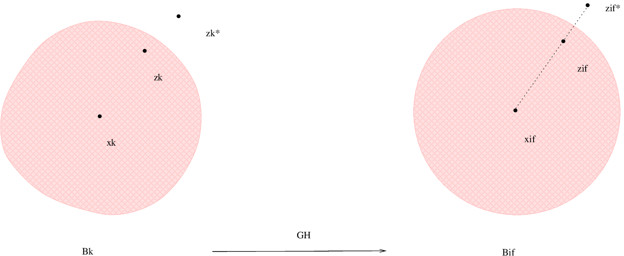
By continuity, for proving (34) in B⁡(z∞,1)B(z_{\infty},1), it suffices to show (34) for every z∈B⁡(x∞,1)\{x∞}z\in B(x_{\infty},1)\backslash\left\{x_{\infty}\right\}. Without loss of generality, we fix an arbitrary point z∈B⁡(x∞,1)\{x∞}z\in B(x_{\infty},1)\backslash\left\{x_{\infty}\right\}. Suppose zk∈B⁡(xk,1)z_{k}\in B(x_{k},1) and zk→zz_{k}\to z, zk∗∈Xkz_{k}^{*}\in X_{k} and zk∗→z∗z_{k}^{*}\to z^{*} (See Figure 2).

Refer to caption
Figure 2: Approximation of Green functions

Let dd be the distance function to the point zkz_{k} under the metric gk​(0)g_{k}(0). Note that

Δ​d2−m=(2−m)​d−m​(1−m+d​Δ​d).\displaystyle\Delta d^{2-m}=(2-m)d^{-m}\left(1-m+d\Delta d\right). (35)

If the underlying space is Euclidean, then the right hand side is equal to 00 whenever d>0d>0. Now on XkX_{k}, we are focusing our attention around the point xkx_{k}, where R​i​c≥−(m−1)​δk4Ric\geq-(m-1)\delta_{k}^{4}. Clearly, Laplacian comparison theorem (c.f. Corollary 1.131 of [13]) implies that

Δ​d2−m+(m−2)​(m−1)​d1−m​δk2≥0\displaystyle\Delta d^{2-m}+(m-2)(m-1)d^{1-m}\delta_{k}^{2}\geq 0 (36)

on B⁡(xk,10)B(x_{k},10). It follows that

0≤∫B⁡(xk,1)\B⁡(zk,r){Δ​d2−m+(m−2)​(m−1)​d1−m​δk2}\displaystyle 0\leq\int_{B(x_{k},1)\backslash B(z_{k},r)}\left\{\Delta d^{2-m}+(m-2)(m-1)d^{1-m}\delta_{k}^{2}\right\}
≤∫B⁡(zk,2)\B⁡(zk,r){Δ​d2−m+(m−2)​(m−1)​d1−m​δk2}\displaystyle\leq\int_{B(z_{k},2)\backslash B(z_{k},r)}\left\{\Delta d^{2-m}+(m-2)(m-1)d^{1-m}\delta_{k}^{2}\right\}
=(m−2)​{|∂B⁡(zk,2)|​21−m−|∂B⁡(zk,r)|​r1−m}+(m−2)​(m−1)​δk2​∫r2(ρ1−m​|∂B⁡(zk,ρ)|)​𝑑ρ\displaystyle=(m-2)\left\{|\partial B(z_{k},2)|2^{1-m}-|\partial B(z_{k},r)|r^{1-m}\right\}+(m-2)(m-1)\delta_{k}^{2}\int_{r}^{2}\left(\rho^{1-m}|\partial B(z_{k},\rho)|\right)d\rho
<(m−2)​{||∂B⁡(zk,2)​|21−m−|​∂B⁡(zk,r)|​r1−m|+4​(m−1)​m​ωm​δk2}.\displaystyle<(m-2)\left\{\left||\partial B(z_{k},2)|2^{1-m}-|\partial B(z_{k},r)|r^{1-m}\right|+4(m-1)m\omega_{m}\delta_{k}^{2}\right\}.

Consequently, we have

∫B⁡(xk,1)\B⁡(zk,r)|Δ​d2−m|\displaystyle\quad\int_{B(x_{k},1)\backslash B(z_{k},r)}\left|\Delta d^{2-m}\right|
≤∫B⁡(xk,1)\B⁡(zk,r)|Δ​d2−m+(m−2)​(m−1)​d1−m​δk2|+∫B⁡(xk,1)\B⁡(zk,r)(m−2)​(m−1)​d1−m​δk2\displaystyle\leq\int_{B(x_{k},1)\backslash B(z_{k},r)}\left|\Delta d^{2-m}+(m-2)(m-1)d^{1-m}\delta_{k}^{2}\right|+\int_{B(x_{k},1)\backslash B(z_{k},r)}(m-2)(m-1)d^{1-m}\delta_{k}^{2}
<(m−2)​{||∂B⁡(zk,2)​|21−m−|​∂B⁡(zk,r)|​r1−m|+8​(m−1)​m​ωm​δk2}.\displaystyle<(m-2)\left\{\left||\partial B(z_{k},2)|2^{1-m}-|\partial B(z_{k},r)|r^{1-m}\right|+8(m-1)m\omega_{m}\delta_{k}^{2}\right\}.

Fix kk, let r→0r\to 0, we have

∫B⁡(xk,1)\{zk}|Δ​d2−m|≤(m−2)​{||∂B⁡(zk,2)|​21−m−m​ωm|+8​(m−1)​m​ωm​δk2}.\displaystyle\int_{B(x_{k},1)\backslash\left\{z_{k}\right\}}\left|\Delta d^{2-m}\right|\leq(m-2)\left\{\left||\partial B(z_{k},2)|2^{1-m}-m\omega_{m}\right|+8(m-1)m\omega_{m}\delta_{k}^{2}\right\}.

Therefore, we obtain

∫B⁡(xk,1)\{zk}|φk​Δ​d2−m|≤C1​(m−2)​{||∂B⁡(zk,2)|​21−m−m​ωm|+8​(m−1)​m​ωm​δk2}→0,\displaystyle\int_{B(x_{k},1)\backslash\left\{z_{k}\right\}}\left|\varphi_{k}\Delta d^{2-m}\right|\leq C_{1}(m-2)\left\{\left||\partial B(z_{k},2)|2^{1-m}-m\omega_{m}\right|+8(m-1)m\omega_{m}\delta_{k}^{2}\right\}\to 0, (37)

as k→∞k\to\infty, since the limit space X∞X_{\infty} is Euclidean, where every geodesic sphere has the same volume ratio: m​ωmm\omega_{m}. Consequently, we can calculate

∫B⁡(xk,1)d2−m​(zk,y)​Δ​φk​(y)​𝑑y\displaystyle\int_{B(x_{k},1)}d^{2-m}(z_{k},y)\Delta\varphi_{k}(y)dy =∫B⁡(xk,1)\{zk}d2−m​(zk,y)​Δ​φk​(y)​𝑑y\displaystyle=\int_{B(x_{k},1)\backslash\left\{z_{k}\right\}}d^{2-m}(z_{k},y)\Delta\varphi_{k}(y)dy
=limr→0∫B⁡(xk,1)\B⁡(zk,r)d2−m​(zk,y)​Δ​φk​(y)​𝑑y\displaystyle=\lim_{r\to 0}\int_{B(x_{k},1)\backslash B(z_{k},r)}d^{2-m}(z_{k},y)\Delta\varphi_{k}(y)dy
=(m−2)​m​ωm​φk​(zk)+∫B⁡(xk,1)\{zk}φk​(y)​Δ​d2−m​(zk,y)​𝑑y.\displaystyle=(m-2)m\omega_{m}\varphi_{k}(z_{k})+\int_{B(x_{k},1)\backslash\left\{z_{k}\right\}}\varphi_{k}(y)\Delta d^{2-m}(z_{k},y)dy. (38)

Of course, the default measure in the calculation is d​y=d​μgk​(0)dy=d\mu_{g_{k}(0)}. Combining (37) and (38), we have

limk→∞∫B⁡(xk,1)d2−m​(zk,y)​Δ​φk​(y)​𝑑y=(m−2)​m​ωm​φ∞​(z).\displaystyle\lim_{k\to\infty}\int_{B(x_{k},1)}d^{2-m}(z_{k},y)\Delta\varphi_{k}(y)dy=(m-2)m\omega_{m}\varphi_{\infty}(z). (39)

Note that d⁡(zk∗,⋅)>0d(z_{k}^{*},\cdot)>0 uniformly on B⁡(xk,1)B(x_{k},1). By similar but simpler arguments, we obtain

limk→∞∫B⁡(xk,1)d2−m​(zk∗,y)​Δ​φk​(y)​𝑑y=0.\displaystyle\lim_{k\to\infty}\int_{B(x_{k},1)}d^{2-m}(z_{k}^{*},y)\Delta\varphi_{k}(y)dy=0. (40)

In view of (39) and (40), we have

(m−2)​m​ωm​φ∞​(z)\displaystyle\quad(m-2)m\omega_{m}\varphi_{\infty}(z)
=limk→∞∫B⁡(xk,1){d2−m​(zk,y)−d2−m​(xk,zk)​d2−m​(zk∗,y)}​Δ​φk​(y)​𝑑y\displaystyle=\lim_{k\to\infty}\int_{B(x_{k},1)}\left\{d^{2-m}(z_{k},y)-d^{2-m}(x_{k},z_{k})d^{2-m}(z_{k}^{*},y)\right\}\Delta\varphi_{k}(y)dy
=limk→∞∫B⁡(xk,1){d2−m​(zk,y)−d2−m​(xk,zk)​d2−m​(zk∗,y)}​(m+m​log⁡2​π+λk2+log⁡φk​(y))​φk​(y)​𝑑y\displaystyle=\lim_{k\to\infty}\int_{B(x_{k},1)}\left\{d^{2-m}(z_{k},y)-d^{2-m}(x_{k},z_{k})d^{2-m}(z_{k}^{*},y)\right\}\left(\frac{m+m\log\sqrt{2\pi}+\lambda_{k}}{2}+\log\varphi_{k}(y)\right)\varphi_{k}(y)dy
=∫B⁡(x∞,1){d2−m​(z,y)−d2−m​(x∞,z)​d2−m​(z∗,y)}⋅(m+m​log⁡2​π+λ∞2+log⁡φ∞​(y))​φ∞​(y)​𝑑y\displaystyle=\int_{B(x_{\infty},1)}\left\{d^{2-m}(z,y)-d^{2-m}(x_{\infty},z)d^{2-m}(z^{*},y)\right\}\cdot\left(\frac{m+m\log\sqrt{2\pi}+\lambda_{\infty}}{2}+\log\varphi_{\infty}(y)\right)\varphi_{\infty}(y)dy
=(m−2)​m​ωm​∫B⁡(x∞,1)G⁡(z,y)⋅(m+m​log⁡2​π+λ∞2+log⁡φ∞​(y))​φ∞​(y)​𝑑y.\displaystyle=(m-2)m\omega_{m}\int_{B(x_{\infty},1)}G(z,y)\cdot\left(\frac{m+m\log\sqrt{2\pi}+\lambda_{\infty}}{2}+\log\varphi_{\infty}(y)\right)\varphi_{\infty}(y)dy.

In the third step, we used the Euler-Lagrangian equation for φk\varphi_{k}. In the fourth step, we used the integrability of d2−md^{2-m} and uniform bound of φk\varphi_{k}. Therefore, we prove (34) for zz. By the arbitrariness of z∈B⁡(x∞,1)\{x∞}z\in B(x_{\infty},1)\backslash\left\{x_{\infty}\right\} and continuity, equation (34), henceforth (33) follows directly. Then the standard bootstrapping argument for elliptic PDEs implies that φ∞∈C∞​(B⁡(x∞,1))\varphi_{\infty}\in C^{\infty}\left(B(x_{\infty},1)\right). This finishes the proof of Claim 2.

Now we are ready to prove the theorem by a contradiction argument. In fact, since ∂B⁡(x∞,1)\partial B(x_{\infty},1) is smooth and φ|∂B⁡(x∞,1)≡0\varphi|_{\partial B(x_{\infty},1)}\equiv 0 (Claim 1), by trivial extension, we can regard φ∞∈W01,2​(ℝm)\varphi_{\infty}\in W_{0}^{1,2}(\mathbb{R}^{m}) (c.f. Section 5.5 of [19]). It follows from the Logarithm Sobolev inequality of Euclidean space (c.f. [22]) that

∫ℝm(12​|∇φ∞|2−2​φ∞2​log⁡φ∞−m⁡(1+log⁡2​π)​φ∞2)≥0.\displaystyle\int_{\mathbb{R}^{m}}\left(\frac{1}{2}|\nabla\varphi_{\infty}|^{2}-2\varphi_{\infty}^{2}\log\varphi_{\infty}-m\left(1+\log\sqrt{2\pi}\right)\varphi_{\infty}^{2}\right)\geq 0. (41)

On the other hand, by (33) in Claim 2 and the fact φ∞≡0\varphi_{\infty}\equiv 0 outside B⁡(x∞,1)B(x_{\infty},1), we deduce that

∫ℝm(12​|∇φ∞|2−2​φ∞2​log⁡φ∞−m⁡(1+log⁡2​π)​φ∞2)=λ∞≤−η<0,\displaystyle\int_{\mathbb{R}^{m}}\left(\frac{1}{2}|\nabla\varphi_{\infty}|^{2}-2\varphi_{\infty}^{2}\log\varphi_{\infty}-m\left(1+\log\sqrt{2\pi}\right)\varphi_{\infty}^{2}\right)=\lambda_{\infty}\leq-\eta<0,

which contradicts to (41)! ∎

Remark 3.1.

If the “almost-Euclidean volume ratio” (inequality (12)) and “almost nonnegative Ricci” (inequality (11)) hold globally, then the rough curvature estimate (inequality (14)) follows from the combination of Perelman’s pseudo-locality theorem and Levy-Gromov inequality(c.f. [21]), whose proof requires some regularity results in geometric measure theory on closed manifolds. There should exist another proof of Proposition 3.1 from some local version of the Gromov-Ivey inequality. However, it seems that some local regularity results in geometric measure theory are required.

Remark 3.2.

Except inequality (11), the “almost nonnegative Ricci” condition can also be interpreted as the LpL^{p}-integration of negative Ricci part is sufficiently small(c.f. [31], [32]), for some p>m2p>\frac{m}{2}. Using this interpretation, one can obtain another pseudo-locality theorem.

Combine Proposition 3.1 with the fundamental work of [7], we obtain the following property.

Proposition 3.2.

There exists a constant δ0=δ0​(m)\delta_{0}=\delta_{0}(m) with the following properties.

Suppose {(X,g(t)),0≤t≤1}\left\{(X,g(t)),0\leq t\leq 1\right\} is a Ricci flow solution, x0∈X,Ω=Bg⁡(0)​(x0,1)x_{0}\in X,\Omega=B_{g(0)}(x_{0},1). Suppose that

R​i​c​(x,0)≥−(m−1)​δ0,∀x∈Ω;|Ω|d​μg⁡(0)≥(1−δ0)​ωm.\displaystyle Ric(x,0)\geq-(m-1)\delta_{0},\quad\forall\;x\in\Omega;\quad|\Omega|_{d\mu_{g(0)}}\geq(1-\delta_{0})\omega_{m}. (42)

Then we have

|Bg⁡(s)​(x,s)|d​μg⁡(s)≥κ′​sm2,|R​m~|​(x,s)≤1100​s−1,∀x∈Ω′=Bg⁡(0)​(x0,34),s∈(0,2​δ0],\displaystyle\left|B_{g(s)}\left(x,\sqrt{s}\right)\right|_{d\mu_{g(s)}}\geq\kappa^{\prime}s^{\frac{m}{2}},\quad\left|\widetilde{Rm}\right|(x,s)\leq\frac{1}{100}s^{-1},\quad\forall\;x\in\Omega^{\prime}=B_{g(0)}\left(x_{0},\frac{3}{4}\right),\;s\in(0,2\delta_{0}],

where κ′=κ′​(m)\kappa^{\prime}=\kappa^{\prime}(m) is a universal constant.

Proof.

Let’s first prove the following Claim.

Claim 3.

For every small ξ>0\xi>0, there exists a number η=η⁡(m,ξ)\eta=\eta(m,\xi) with the following property.

Suppose R​i​c​(x,0)≥−(m−1)​ηRic(x,0)\geq-(m-1)\eta in Ω=Bg⁡(0)​(x0,1)\Omega=B_{g(0)}(x_{0},1), and |Ω|d​μg⁡(0)≥(1−η)​ωm|\Omega|_{d\mu_{g(0)}}\geq(1-\eta)\omega_{m}, then

8m​|Bg⁡(0)​(y,18)|d​μg⁡(0)≥(1−ξ)​ωm,∀y∈Bg⁡(0)​(x0,34).\displaystyle 8^{m}\left|B_{g(0)}\left(y,\frac{1}{8}\right)\right|_{d\mu_{g(0)}}\geq(1-\xi)\omega_{m},\quad\forall\;y\in B_{g(0)}\left(x_{0},\frac{3}{4}\right). (43)

Actually, if this statement was wrong, we can find a sequence of ηi→0\eta_{i}\to 0 and manifolds (Xi,xi,gi​(0))(X_{i},x_{i},g_{i}(0)) such that (42) holds for ηi\eta_{i} and the ball Ωi=Bgi​(0)​(xi,1)\Omega_{i}=B_{g_{i}(0)}(x_{i},1). However, for some point yi∈Bgi​(0)​(xi,34)y_{i}\in B_{g_{i}(0)}\left(x_{i},\frac{3}{4}\right), we have

8m​|Bgi​(0)​(yi,18)|d​μgi​(0)<(1−ξ)​ωm.\displaystyle 8^{m}\left|B_{g_{i}(0)}\left(y_{i},\frac{1}{8}\right)\right|_{d\mu_{g_{i}(0)}}<\left(1-\xi\right)\omega_{m}. (44)

Suppose (Ωi,xi,gi​(0))\left(\Omega_{i},x_{i},g_{i}(0)\right) converges to (Ω¯,x¯,g¯)\left(\bar{\Omega},\bar{x},\bar{g}\right). Clearly, we see that Ω¯\bar{\Omega} is isometric to the unit ball in the Euclidean space ℝm\mathbb{R}^{m}. Since yi∈Bgi​(0)​(xi,34)y_{i}\in B_{g_{i}(0)}\left(x_{i},\frac{3}{4}\right), we can assume yi→y¯∈B⁡(x¯,34+1100)⊂Ω¯y_{i}\to\bar{y}\in B\left(\bar{x},\frac{3}{4}+\frac{1}{100}\right)\subset\bar{\Omega}. The lower bound of Ricci guarantees the continuity of volume. Therefore we have

limi→∞8m​|Bgi​(0)​(yi,18)|d​μgi​(0)=8m​|Bg¯​(y¯,18)|d​μg¯=ωm,\displaystyle\lim_{i\to\infty}8^{m}\left|B_{g_{i}(0)}\left(y_{i},\frac{1}{8}\right)\right|_{d\mu_{g_{i}(0)}}=8^{m}\left|B_{\bar{g}}\left(\bar{y},\frac{1}{8}\right)\right|_{d\mu_{\bar{g}}}=\omega_{m},

which contradicts to (44)! This contradiction establishes the proof of Claim 3.

Let ξ=δ4​(m,11000​m)\xi=\delta^{4}\left(m,\frac{1}{1000m}\right), where δ\delta is defined by Proposition 3.1. Let η=η⁡(m,ξ)\eta=\eta(m,\xi) according to Claim 3.

Suppose the conditions of Claim 3 is satisfied for η=η⁡(m,ξ)\eta=\eta(m,\xi). Define g^​(t)=ξ−2​g​(ξ2​t)\hat{g}(t)=\xi^{-2}g(\xi^{2}t). Fix an arbitrary point y∈Bg⁡(0)​(x0,34)y\in B_{g(0)}\left(x_{0},\frac{3}{4}\right). By volume comparison, inequality (43) and the choice of ξ\xi yield that (X,y,g^​(0))(X,y,\hat{g}(0)) satisfies the initial conditions of Proposition 3.1. In particular, we have |Bg^​(t)​(y,t)|d​μg^​(t)≥κ′​tm2,|R​m|g^​(t)​(y)≤11000​m​t+ϵ−2\displaystyle\left|B_{\hat{g}(t)}\left(y,\sqrt{t}\right)\right|_{d\mu_{\hat{g}(t)}}\geq\kappa^{\prime}t^{\frac{m}{2}},\quad|Rm|_{\hat{g}(t)}(y)\leq\frac{1}{1000mt}+\epsilon^{-2} for every t∈(0,ϵ2]t\in\left(0,\epsilon^{2}\right]. This implies that for every t∈(0,ϵ2200]t\in\left(0,\frac{\epsilon^{2}}{200}\right], we have

|Bg^​(t)​(y,t)|d​μg^​(t)≥κ′​tm2,|R​m|g^​(t)​(y)≤1100​t.\displaystyle\left|B_{\hat{g}(t)}\left(y,\sqrt{t}\right)\right|_{d\mu_{\hat{g}(t)}}\geq\kappa^{\prime}t^{\frac{m}{2}},\quad|Rm|_{\hat{g}(t)}(y)\leq\frac{1}{100t}.

By a trivial rescaling argument, we conclude

|Bg⁡(t)​(y,t)|d​μg⁡(t)≥κ′​tm2,|R​m|g⁡(t)​(y)≤1100​t,∀t∈(0,ξ2​ϵ2200].\displaystyle\left|B_{g(t)}\left(y,\sqrt{t}\right)\right|_{d\mu_{g(t)}}\geq\kappa^{\prime}t^{\frac{m}{2}},\quad|Rm|_{g(t)}(y)\leq\frac{1}{100t},\quad\forall\;t\in\left(0,\frac{\xi^{2}\epsilon^{2}}{200}\right].

Define δ0≜min⁡{ξ2​ϵ21000,η⁡(m,ξ)}\delta_{0}\triangleq\min\left\{\frac{\xi^{2}\epsilon^{2}}{1000},\eta(m,\xi)\right\}. Clearly, Proposition 3.2 holds for this choice of δ0\delta_{0}. ∎

Now we are ready to prove the pseudo-locality theorem under the normalized Ricci flow.

Theorem 3.1 (Pseudo-locality theorem).

There exists a constant δ0=δ0​(m)\delta_{0}=\delta_{0}(m) with the following properties.

Suppose {(X,g(t)),0≤t≤1}\left\{(X,g(t)),0\leq t\leq 1\right\} is a normalized Ricci flow solution: ∂∂t​g=−R​i​c+λ0​g\frac{\partial{}}{\partial{t}}g=-Ric+\lambda_{0}g, λ0\lambda_{0} is a constant with |λ0|≤1|\lambda_{0}|\leq 1. Let x0∈X,Ω=Bg⁡(0)​(x0,1)x_{0}\in X,\Omega=B_{g(0)}(x_{0},1). Suppose that

R​i​c​(x,0)≥−(m−1)​δ0,∀x∈Ω;|Ω|d​μg⁡(0)≥(1−δ0)​ωm.\displaystyle Ric(x,0)\geq-(m-1)\delta_{0},\quad\forall\;x\in\Omega;\quad|\Omega|_{d\mu_{g(0)}}\geq(1-\delta_{0})\omega_{m}. (45)

Then we have

|Bg⁡(t)​(x,t)|d​μg⁡(t)≥κ0​tm2,\displaystyle\left|B_{g(t)}\left(x,\sqrt{t}\right)\right|_{d\mu_{g(t)}}\geq\kappa_{0}t^{\frac{m}{2}}, (46)
|R​m|​(x,t)≤t−1,∀x∈Ω′=Bg⁡(0)​(x0,34),t∈(0,2​δ0],\displaystyle|Rm|(x,t)\leq t^{-1},\quad\forall\;x\in\Omega^{\prime}=B_{g(0)}\left(x_{0},\frac{3}{4}\right),\;t\in(0,2\delta_{0}], (47)

where κ0=κ0​(m)\kappa_{0}=\kappa_{0}(m) is a universal constant.

Proof.

Let g~​(s)=(1−2​λ0​s)​g​(log⁡(1−2​λ0​s)−λ0)\tilde{g}(s)=\left(1-2\lambda_{0}s\right)g\left(\frac{\log(1-2\lambda_{0}s)}{-\lambda_{0}}\right). Clearly, g~​(s)\tilde{g}(s) is a Ricci flow solution with g~​(0)=g​(0)\tilde{g}(0)=g(0). Denote log⁡(1−2​λ0​s)−λ0\frac{\log(1-2\lambda_{0}s)}{-\lambda_{0}} by t⁡(s)t(s). Then we have g~​(s)=(1−2​λ0​s)​g​(t)\tilde{g}(s)=\left(1-2\lambda_{0}s\right)g(t). By Taylor expansion of t⁡(s)=log⁡(1−2​λ0​s)−λ0t(s)=\frac{\log(1-2\lambda_{0}s)}{-\lambda_{0}}, shrink δ0\delta_{0} if necessary, we have 32​s<t<3​s\frac{3}{2}s<t<3s whenever s∈(0,10​δ0)s\in(0,10\delta_{0}). Note that

g⁡(t)=eλ0​t​g~​(1−e−λ0​t2​λ0)=eλ0​t​g~​(s),\displaystyle g(t)=e^{\lambda_{0}t}\tilde{g}\left(\frac{1-e^{-\lambda_{0}t}}{2\lambda_{0}}\right)=e^{\lambda_{0}t}\tilde{g}(s),

which implies

Bg⁡(t)​(x,t)=Beλ0​t​g~​(s)​(x,t)=Bg~​(s)​(x,e−λ0​t​t).\displaystyle B_{g(t)}\left(x,\sqrt{t}\right)=B_{e^{\lambda_{0}t}\tilde{g}(s)}\left(x,\sqrt{t}\right)=B_{\tilde{g}(s)}\left(x,\sqrt{e^{-\lambda_{0}t}t}\right).

If t∈(0,2​δ0]t\in(0,2\delta_{0}], then s∈(0,43​δ0]s\in\left(0,\frac{4}{3}\delta_{0}\right]. Note that g~​(0)=g​(0)\tilde{g}(0)=g(0). Therefore, Proposition 3.2 can be applied to obtain the following estimates.

{|Bg⁡(t)​(x,t)|d​μg⁡(t)=em​λ0​t2​|Bg~​(s)​(x,e−λ0​t​t)|d​μg~​(s)>12​|Bg~​(s)​(x,s)|d​μg~​(s)>12​κ′​sm2≜κ0​tm2,|R​m|​(x,t)=e−λ0​t​|R​m~|​(x,s)≤e−λ0​t100​s−1<3100​e−λ0​t​t−1<t−1,\displaystyle\begin{cases}&\left|B_{g(t)}\left(x,\sqrt{t}\right)\right|_{d\mu_{g(t)}}=e^{\frac{m\lambda_{0}t}{2}}\left|B_{\tilde{g}(s)}\left(x,\sqrt{e^{-\lambda_{0}t}t}\right)\right|_{d\mu_{\tilde{g}(s)}}>\frac{1}{2}\left|B_{\tilde{g}(s)}\left(x,\sqrt{s}\right)\right|_{d\mu_{\tilde{g}(s)}}>\frac{1}{2}\kappa^{\prime}s^{\frac{m}{2}}\triangleq\kappa_{0}t^{\frac{m}{2}},\\ &|Rm|(x,t)=e^{-\lambda_{0}t}\left|\widetilde{Rm}\right|(x,s)\leq\frac{e^{-\lambda_{0}t}}{100}s^{-1}<\frac{3}{100}e^{-\lambda_{0}t}t^{-1}<t^{-1},\end{cases}

for every point x∈Ω′=Bg⁡(0)​(x0,34),t∈(0,2​δ0]x\in\Omega^{\prime}=B_{g(0)}\left(x_{0},\frac{3}{4}\right),\;t\in(0,2\delta_{0}]. So we finish the proof of Theorem 3.1. ∎

4 Curvature, distance and volume estimates

Under the Ricci flow, evolution of distance between two points is controlled by the Ricci curvature. By maximum principle, a scalar-flat Ricci flow solution must be Ricci flat. Therefore, the distance between any two points does not depend on the time. In this section, we will develop an “almost”-version of this observation. Fix two points in the underlying manifold of a normalized Ricci flow solution. If the normalized scalar curvature is almost zero in the L1L^{1}-sense, then the distance between these two points are almost fixed by the flow. This new estimate is based on Proposition 2.1, Theorem 3.1, and the following estimate of normalized Ricci curvature.

Lemma 4.1.

Suppose {(X,x0,g(t)),−2≤t≤1}\left\{(X,x_{0},g(t)),-2\leq t\leq 1\right\} satisfies the following conditions.

  • •

    g⁡(t)g(t) satisfies the normalized Ricci flow solution

    ∂∂t​gi​j=−Ri​j+λ0​gi​j\displaystyle\frac{\partial{}}{\partial{t}}g_{ij}=-R_{ij}+\lambda_{0}g_{ij}

    where λ0\lambda_{0} is a constant with |λ0|≤1100​m2|\lambda_{0}|\leq\frac{1}{100m^{2}}. 11 1 Note that this is not 11. In our mind, the flow in this lemma comes from the blowup of a general normalized flow, so the coefficient λ0\lambda_{0} could be very small.

  • •

    |R​m|​(x,t)≤1100​m2|Rm|(x,t)\leq\frac{1}{100m^{2}} whenever x∈Bg⁡(t)​(x0,100),t∈[−2,1]x\in B_{g(t)}(x_{0},100),\;t\in[-2,1].

  • •

    i​n​j​(x0,t)≥100inj(x_{0},t)\geq 100 uniformly for every t∈[−2,1]t\in[-2,1].

Then there exists a large constant C=C⁡(m)C=C(m) such that

|R​i​c−λ0​g|​(x0,0)≤C​{∫−21∫Bg⁡(0)​(x0,10)|R−m​λ0|​𝑑μ​𝑑t}12.\displaystyle|Ric-\lambda_{0}g|(x_{0},0)\leq C\left\{\int_{-2}^{1}\int_{B_{g(0)}(x_{0},10)}|R-m\lambda_{0}|d\mu dt\right\}^{\frac{1}{2}}. (48)
Proof.

For simplicity of notation, we denote R​i​c−λ0​gRic-\lambda_{0}g by hh, denote R−m​λ0R-m\lambda_{0} by HH.

Recall that |h||h| satisfies inequality (4). Locally, |R​m||Rm| is uniformly bounded. So we should be able to control the L∞L^{\infty}-norm of |h||h| by the L2L^{2}-norm of |h||h|. Actually, define Ω=Bg⁡(0)​(x0,1),Ω′=Bg⁡(0)​(x0,12)\Omega=B_{g(0)}(x_{0},1),\;\Omega^{\prime}=B_{g(0)}\left(x_{0},\frac{1}{2}\right), D=Ω×[−1,0]D=\Omega\times[-1,0], D′=Ω′×[−12,0].D^{\prime}=\Omega^{\prime}\times[-\frac{1}{2},0]. By the second and the third condition, we obtain that (Ω,g⁡(t))(\Omega,g(t)) has a uniform Sobolev constant σ=σ⁡(m)\sigma=\sigma(m). Similar to Theorem 3.2 of [43], Moser iteration for the term h=R​i​c−λ0​gh=Ric-\lambda_{0}g implies

supD′|h|≤C⁡(m)​{∬D|h|2​𝑑μ​𝑑t}12.\displaystyle\sup_{D^{\prime}}|h|\leq C(m)\left\{\iint_{D}|h|^{2}d\mu dt\right\}^{\frac{1}{2}}. (49)

Choose cutoff function η~​(y,t)=ψ⁡(dg⁡(t)​(y,x0)−2)\tilde{\eta}(y,t)=\psi(d_{g(t)}(y,x_{0})-2), where ψ\psi is a smooth function which achieves value 11 on (−∞,0](-\infty,0] and 00 on [1,∞)[1,\infty), which also satisfies |ψ′|≤2|\psi^{\prime}|\leq 2. Recall that |λ0|≤1100​m2|\lambda_{0}|\leq\frac{1}{100m^{2}}. So we have

h⁡(V,V)≤(m−1100​m2+|λ0|)​g​(V,V)≤1100​m​g​(V,V)\displaystyle h(V,V)\leq\left(\frac{m-1}{100m^{2}}+|\lambda_{0}|\right)g(V,V)\leq\frac{1}{100m}g(V,V)

whenever V∈T​XV\in TX and |R​m|​(V,V)≤1100​m2​g​(V,V)|Rm|(V,V)\leq\frac{1}{100m^{2}}g(V,V). By the evolution of geodesic length, it is easy to check that

Ω=Bg⁡(0)​(x0,1)⊂Bg⁡(t)​(x0,2),\displaystyle\Omega=B_{g(0)}(x_{0},1)\subset B_{g(t)}(x_{0},2),
Bg⁡(t)​(x0,3)⊂W=Bg⁡(0)​(x0,10),\displaystyle B_{g(t)}(x_{0},3)\subset W=B_{g(0)}(x_{0},10),

for every −2≤t≤1-2\leq t\leq 1. Therefore η~≡1\tilde{\eta}\equiv 1 on Ω\Omega, η~≡0\tilde{\eta}\equiv 0 outside WW whenever −2≤t≤1-2\leq t\leq 1.

By mean value theorem of calculus, we can assume t1,t2t_{1},t_{2} satisfies the following properties.

−2≤t1≤−1,\displaystyle-2\leq t_{1}\leq-1, ∫W|H|𝑑μ|t1≤∫−2−1∫W|H|​𝑑μ​𝑑t≤∫−21∫W|H|​𝑑μ​𝑑t.\displaystyle\quad\left.\int_{W}|H|d\mu\right|_{t_{1}}\leq\int_{-2}^{-1}\int_{W}|H|d\mu dt\leq\int_{-2}^{1}\int_{W}|H|d\mu dt. (50)
0≤t2≤1,\displaystyle 0\leq t_{2}\leq 1, ∫W|H|𝑑μ|t2≤∫01∫W|H|​𝑑μ​𝑑t≤∫−21∫W|H|​𝑑μ​𝑑t.\displaystyle\quad\left.\int_{W}|H|d\mu\right|_{t_{2}}\leq\int_{0}^{1}\int_{W}|H|d\mu dt\leq\int_{-2}^{1}\int_{W}|H|d\mu dt. (51)

Using the evolution equation of normalized scalar curvature equation (5), similar to the calculation in [43], we obtain that

∫t1t2∫Ω|h|2​𝑑μ​𝑑t\displaystyle\quad\int_{t_{1}}^{t_{2}}\int_{\Omega}|h|^{2}d\mu dt
≤∫t1t2∫Xη~​|h|2​𝑑μ​𝑑t\displaystyle\leq\int_{t_{1}}^{t_{2}}\int_{X}\tilde{\eta}|h|^{2}d\mu dt
=∫t1t2∫Xη~​(∂H∂t−12​Δ​H−λ0​H)​𝑑μ​𝑑t\displaystyle=\int_{t_{1}}^{t_{2}}\int_{X}\tilde{\eta}\left(\frac{\partial{H}}{\partial{t}}-\frac{1}{2}\Delta H-\lambda_{0}H\right)d\mu dt
=(∫Xη~​H​𝑑μ)|t1t2−∫t1t2∫XH⁡(∂∂t​η~+12​Δ​η~+(λ0−H2)​η~)​𝑑μ​𝑑t\displaystyle=\left.\left(\int_{X}\tilde{\eta}Hd\mu\right)\right|_{t_{1}}^{t_{2}}-\int_{t_{1}}^{t_{2}}\int_{X}H\left(\frac{\partial{}}{\partial{t}}\tilde{\eta}+\frac{1}{2}\Delta\tilde{\eta}+\left(\lambda_{0}-\frac{H}{2}\right)\tilde{\eta}\right)d\mu dt
≤C⁡{∫W|H|​𝑑μ|t=t2+∫W|H|​𝑑μ|t=t1+∫t1t2∫W|H|​𝑑μ​𝑑t}.\displaystyle\leq C\left\{\left.\int_{W}|H|d\mu\right|_{t=t_{2}}+\left.\int_{W}|H|d\mu\right|_{t=t_{1}}+\int_{t_{1}}^{t_{2}}\int_{W}|H|d\mu dt\right\}. (52)

Note that [−1,0]⊂[t1,t2]⊂[−2,1][-1,0]\subset[t_{1},t_{2}]\subset[-2,1]. Combining (49), (50), (51) and (52) yields

supD′|h|≤C​{∬D|h|2​𝑑μ​𝑑t}12≤C​{∫−21∫W|H|​𝑑μ​𝑑t}12,\displaystyle\sup_{D^{\prime}}|h|\leq C\left\{\iint_{D}|h|^{2}d\mu dt\right\}^{\frac{1}{2}}\leq C\left\{\int_{-2}^{1}\int_{W}|H|d\mu dt\right\}^{\frac{1}{2}}, (53)

where CC depends only on the dimension mm. ∎

Combine Lemma 4.1 and Theorem 3.1, we have the following estimate.

Lemma 4.2.

Suppose {(X,x0,g(t)),0≤t≤1}\left\{(X,x_{0},g(t)),0\leq t\leq 1\right\} satisfies all the conditions in Theorem 3.1. Then

|R​i​c−λ0​g|​(x,s)≤C⁡(m)​s−m+42​{∫02​s∫Ω|R−m​λ0|​𝑑μ​𝑑t}12,∀x∈Ω′=Bg⁡(0)​(x0,12),s∈(0,δ0].\displaystyle|Ric-\lambda_{0}g|(x,s)\leq C(m)s^{-\frac{m+4}{2}}\left\{\int_{0}^{2s}\int_{\Omega}|R-m\lambda_{0}|d\mu dt\right\}^{\frac{1}{2}},\quad\forall x\in\Omega^{\prime}=B_{g(0)}\left(x_{0},\frac{1}{2}\right),\;s\in\left(0,\delta_{0}\right]. (54)
Proof.

By Theorem 3.1, we have

|R​m|​(x,t)≤t−1,|Bg⁡(t)​(x,t)|d​μg⁡(t)≥κ​(t)m,\displaystyle|Rm|(x,t)\leq t^{-1},\quad\left|B_{g(t)}\left(x,\sqrt{t}\right)\right|_{d\mu_{g(t)}}\geq\kappa\left(\sqrt{t}\right)^{m}, (55)

for every point y∈Bg⁡(0)​(x0,34)y\in B_{g(0)}\left(x_{0},\frac{3}{4}\right), t∈(0,2​δ0]t\in(0,2\delta_{0}].

Fix x∈Ω′=Bg⁡(0)​(x0,12),s∈(0,δ0]x\in\Omega^{\prime}=B_{g(0)}\left(x_{0},\frac{1}{2}\right),\;s\in(0,\delta_{0}]. By (55), the injectivity radius estimate in [12] yields that

i​n​j​(x,t)≥ξ​s,\displaystyle inj(x,t)\geq\xi\sqrt{s}, (56)

for some constant ξ=ξ⁡(m,κ⁡(m))=ξ⁡(m)\xi=\xi(m,\kappa(m))=\xi(m) whenever s2≤t≤2​s\frac{s}{2}\leq t\leq 2s. Put

A=1000​m​ξ−1​s−12,g~​(t)=A2​g​(A−2​t+s).A=1000m\xi^{-1}s^{-\frac{1}{2}},\quad\tilde{g}(t)=A^{2}g\left(A^{-2}t+s\right).

Clearly, g~\tilde{g} satisfies the evolution equation

∂∂t​g~=−R​i​c~+A−2​λ0​g~.\displaystyle\frac{\partial{}}{\partial{t}}\tilde{g}=-\widetilde{Ric}+A^{-2}\lambda_{0}\tilde{g}.

In view of (55) and (56), we have injectivity radius estimate and curvature estimate required by Lemma 4.1. It follows that

|R​i​c~−A−2​λ0​g~|2​(x,0)≤C​∫−12∫Bg~0​(x,10)|R~−m​A−2​λ0|​𝑑μ~​𝑑t,\displaystyle\left|\widetilde{Ric}-A^{-2}\lambda_{0}\tilde{g}\right|^{2}(x,0)\leq C\int_{-1}^{2}\int_{B_{\tilde{g}_{0}}(x,10)}\left|\tilde{R}-mA^{-2}\lambda_{0}\right|d\tilde{\mu}dt,

which is the same as the following inequality before scaling:

|R​i​c−λ0​g|2​(x,s)≤C​Am+4​∫s−A−2s+2​A−2∫Bg⁡(s)​(x,10​A−1)|R−m​λ0|​𝑑μ​𝑑t.\displaystyle|Ric-\lambda_{0}g|^{2}(x,s)\leq CA^{m+4}\int_{s-A^{-2}}^{s+2A^{-2}}\int_{B_{g(s)}\left(x,10A^{-1}\right)}|R-m\lambda_{0}|d\mu dt. (57)

Recall that in the definition A=1000​m​ξ−1​s−12A=1000m\xi^{-1}s^{-\frac{1}{2}}, 1000​m​ξ−11000m\xi^{-1} is a constant depending only on mm. Therefore, (57) implies

|R​i​c−λ0​g|​(x,s)\displaystyle|Ric-\lambda_{0}g|(x,s) ≤C⁡(m)​s−m+42​{∫s−A−2s+2​A−2∫Bg⁡(s)​(x,10​A−1)|R−m​λ0|​𝑑μ​𝑑t}12.\displaystyle\leq C(m)s^{-\frac{m+4}{2}}\left\{\int_{s-A^{-2}}^{s+2A^{-2}}\int_{B_{g(s)}\left(x,10A^{-1}\right)}|R-m\lambda_{0}|d\mu dt\right\}^{\frac{1}{2}}. (58)

By inequality (60), whose proof is independent, we obtain that

Bg⁡(s)​(x,10​A−1)⊂Bg⁡(s)​(x,18−C​s)⊂Bg⁡(0)​(x,18)⊂Bg⁡(0)​(x0,34)⊂Ω=Bg⁡(0)​(x0,1).\displaystyle B_{g(s)}\left(x,10A^{-1}\right)\subset B_{g(s)}\left(x,\frac{1}{8}-C\sqrt{s}\right)\subset B_{g(0)}\left(x,\frac{1}{8}\right)\subset B_{g(0)}\left(x_{0},\frac{3}{4}\right)\subset\Omega=B_{g(0)}\left(x_{0},1\right). (59)

Then inequality (54) follows from (58), (59) and the fact that [s−A−2,s+2​A−2]⊂[0,2​s][s-A^{-2},s+2A^{-2}]\subset[0,2s]. ∎

Recall Proposition 2.1, estimate (54) implies that distance is almost expanding along the flow.

Lemma 4.3.

Suppose {(X,x0,g(t)),0≤t≤1}\left\{(X,x_{0},g(t)),0\leq t\leq 1\right\} satisfies all the conditions in Theorem 3.1. Then for every time t0∈(0,δ0]t_{0}\in(0,\delta_{0}] and every two points x1,x2∈Ω′=Bg⁡(0)​(x0,12)x_{1},x_{2}\in\Omega^{\prime}=B_{g(0)}\left(x_{0},\frac{1}{2}\right), we have

dg⁡(t0)​(x1,x2)≥dg⁡(0)​(x1,x2)−C​t0,\displaystyle d_{g(t_{0})}(x_{1},x_{2})\geq d_{g(0)}(x_{1},x_{2})-C\sqrt{t_{0}}, (60)
dg⁡(δ0)​(x1,x2)≥dg⁡(0)​(x1,x2)−C⁡(t0+t0−m+22​E12),\displaystyle d_{g(\delta_{0})}(x_{1},x_{2})\geq d_{g(0)}(x_{1},x_{2})-C\left(\sqrt{t_{0}}+t_{0}^{-\frac{m+2}{2}}E^{\frac{1}{2}}\right), (61)

where C=C⁡(m)C=C(m) is a universal constant, E=∫02​δ0∫Ω|R−m​λ0|​𝑑μ​𝑑tE=\int_{0}^{2\delta_{0}}\int_{\Omega}|R-m\lambda_{0}|d\mu dt. In particular, if E<δ0m+3E<\delta_{0}^{m+3}, then we have

dg⁡(δ0)​(x1,x2)≥dg⁡(0)​(x1,x2)−C​E12​(m+3).\displaystyle d_{g(\delta_{0})}(x_{1},x_{2})\geq d_{g(0)}(x_{1},x_{2})-CE^{\frac{1}{2(m+3)}}. (62)
Proof.

Let us first prove inequality (60).

By inequality (7) and inequality (47), we have

dd​t​dg⁡(t)​(x1,x2)≥12​λ0​dg⁡(0)​(x1,x2)−C​t−12,∀t∈(0,t0],\displaystyle\frac{d}{dt}d_{g(t)}(x_{1},x_{2})\geq\frac{1}{2}\lambda_{0}d_{g(0)}(x_{1},x_{2})-Ct^{-\frac{1}{2}},\quad\forall t\in(0,t_{0}],

where CC is a universal constant. Consequently, we have

dd​t​(e−λ0​t2​dg⁡(t)​(x1,x2))≥−C​e−λ0​t2​t−12≥−C​t−12,\displaystyle\qquad\frac{d}{dt}\left(e^{-\frac{\lambda_{0}t}{2}}d_{g(t)}(x_{1},x_{2})\right)\geq-Ce^{-\frac{\lambda_{0}t}{2}}t^{-\frac{1}{2}}\geq-Ct^{-\frac{1}{2}},
⇒e−λ0​t02​dg⁡(t0)​(x1,x2)−dg⁡(0)​(x1,x2)≥−C​t0,\displaystyle\Rightarrow e^{-\frac{\lambda_{0}t_{0}}{2}}d_{g(t_{0})}(x_{1},x_{2})-d_{g(0)}(x_{1},x_{2})\geq-C\sqrt{t_{0}},
⇒dg⁡(t0)​(x1,x2)≥eλ0​t02​(dg⁡(0)​(x1,x2)−C​t0).\displaystyle\Rightarrow d_{g(t_{0})}(x_{1},x_{2})\geq e^{\frac{\lambda_{0}t_{0}}{2}}\left(d_{g(0)}(x_{1},x_{2})-C\sqrt{t_{0}}\right).

If λ0≥0\lambda_{0}\geq 0, we have already obtain inequality (60) trivially. If λ0<0\lambda_{0}<0, we have

dg⁡(t0)​(x1,x2)\displaystyle d_{g(t_{0})}(x_{1},x_{2}) ≥(dg⁡(0)​(x1,x2)−C​t0)+(eλ0​t02−1)​(dg⁡(0)​(x1,x2)−C​t0)\displaystyle\geq\left(d_{g(0)}(x_{1},x_{2})-C\sqrt{t_{0}}\right)+\left(e^{\frac{\lambda_{0}t_{0}}{2}}-1\right)\left(d_{g(0)}(x_{1},x_{2})-C\sqrt{t_{0}}\right)
≥(dg⁡(0)​(x1,x2)−C​t0)−C​t0​|dg⁡(0)​(x1,x2)−C​t0|\displaystyle\geq\left(d_{g(0)}(x_{1},x_{2})-C\sqrt{t_{0}}\right)-Ct_{0}\left|d_{g(0)}(x_{1},x_{2})-C\sqrt{t_{0}}\right|
≥(dg⁡(0)​(x1,x2)−C​t0)−C​t0\displaystyle\geq\left(d_{g(0)}(x_{1},x_{2})-C\sqrt{t_{0}}\right)-Ct_{0}
≥dg⁡(0)​(x1,x2)−C​t0.\displaystyle\geq d_{g(0)}(x_{1},x_{2})-C\sqrt{t_{0}}.

So we finish the proof of inequality (60).

We continue to prove inequality (61). Along the normalized Ricci flow, the derivative of logarithm of geodesic length is bounded by the term |R​i​c−λ0​g||Ric-\lambda_{0}g| on the geodesic. Therefore, estimate (54) yields the following inequalities.

|log⁡dg⁡(δ0)​(x1,x2)dg⁡(t0)​(x1,x2)|≤C​∫t0δ0t−m+42​E12​𝑑t≤C​E12​(t0−m+22−δ0−m+22)≤C​E12​t0−m+22.\displaystyle\left|\log\frac{d_{g(\delta_{0})}(x_{1},x_{2})}{d_{g(t_{0})}(x_{1},x_{2})}\right|\leq C\int_{t_{0}}^{\delta_{0}}t^{-\frac{m+4}{2}}E^{\frac{1}{2}}dt\leq CE^{\frac{1}{2}}\left(t_{0}^{-\frac{m+2}{2}}-\delta_{0}^{-\frac{m+2}{2}}\right)\leq CE^{\frac{1}{2}}t_{0}^{-\frac{m+2}{2}}.

It follows that

dg⁡(δ0)​(x1,x2)\displaystyle d_{g(\delta_{0})}(x_{1},x_{2}) ≥dg⁡(t0)​(x1,x2)​e−C​t0−m+22​E12\displaystyle\geq d_{g(t_{0})}(x_{1},x_{2})e^{-Ct_{0}^{-\frac{m+2}{2}}E^{\frac{1}{2}}}
≥(dg⁡(0)​(x1,x2)−C​t012)​e−C​t0−m+22​E12\displaystyle\geq\left(d_{g(0)}(x_{1},x_{2})-Ct_{0}^{\frac{1}{2}}\right)e^{-Ct_{0}^{-\frac{m+2}{2}}E^{\frac{1}{2}}}
=(dg⁡(0)​(x1,x2)−C​t012)+(e−C​t0−m+22​E12−1)⋅(dg⁡(0)​(x1,x2)−C​t012)\displaystyle=\left(d_{g(0)}(x_{1},x_{2})-Ct_{0}^{\frac{1}{2}}\right)+\left(e^{-Ct_{0}^{-\frac{m+2}{2}}E^{\frac{1}{2}}}-1\right)\cdot\left(d_{g(0)}(x_{1},x_{2})-Ct_{0}^{\frac{1}{2}}\right)
≥(dg⁡(0)​(x1,x2)−C​t012)−C​t0−m+22​E12​|dg⁡(0)​(x1,x2)−C​t012|\displaystyle\geq\left(d_{g(0)}(x_{1},x_{2})-Ct_{0}^{\frac{1}{2}}\right)-Ct_{0}^{-\frac{m+2}{2}}E^{\frac{1}{2}}\left|d_{g(0)}(x_{1},x_{2})-Ct_{0}^{\frac{1}{2}}\right|
≥dg⁡(0)​(x1,x2)−C⁡(t012+t0−m+22​E12).\displaystyle\geq d_{g(0)}(x_{1},x_{2})-C\left(t_{0}^{\frac{1}{2}}+t_{0}^{-\frac{m+2}{2}}E^{\frac{1}{2}}\right).

So we finish the proof of inequality (61).

If E<δ0m+3E<\delta_{0}^{m+3}, then E1m+3<δ0E^{\frac{1}{m+3}}<\delta_{0}. Let t0=E1m+3t_{0}=E^{\frac{1}{m+3}} and plug it into inequality (61), we obtain inequality (62). ∎

Corollary 4.1.

Same conditions as in Lemma 4.3. If E<<δ0m+3E<<\delta_{0}^{m+3}, x1∈Ω′=Bg⁡(0)​(x0,12)x_{1}\in\Omega^{\prime}=B_{g(0)}\left(x_{0},\frac{1}{2}\right), then

Bg⁡(δ0)​(x1,r−C​E12​(m+3))⊂Bg⁡(0)​(x1,r),\displaystyle B_{g(\delta_{0})}\left(x_{1},r-CE^{\frac{1}{2(m+3)}}\right)\subset B_{g(0)}\left(x_{1},r\right), (63)

for every 0<r<12−dg⁡(0)​(x0,x1)0<r<\frac{1}{2}-d_{g(0)}(x_{0},x_{1}). In particular, we have

Bg⁡(δ0)​(x0,r−C​E12​(m+3))⊂Bg⁡(0)​(x0,r),∀ 0<r<12.\displaystyle B_{g(\delta_{0})}\left(x_{0},r-CE^{\frac{1}{2(m+3)}}\right)\subset B_{g(0)}\left(x_{0},r\right),\quad\forall\;0<r<\frac{1}{2}. (64)
Proof.

Direct application of inequality (62). ∎

Intuitively, an almost expanding map which almost fix volume must be an almost isometry. This observation can be achieved precisely by Theorem 4.1. However, in order to obtain Theorem 4.1, we first need an estimate to prevent the distance to expand too fast, which is the meaning of the following Lemma.

Lemma 4.4.

Suppose {(X,x0,g(t)),0≤t≤1}\left\{(X,x_{0},g(t)),0\leq t\leq 1\right\} satisfies all the conditions in Theorem 3.1.

Let Ω=Bg⁡(0)​(x0,1),Ω′=Bg⁡(0)​(x0,12)\Omega=B_{g(0)}(x_{0},1),\Omega^{\prime}=B_{g(0)}\left(x_{0},\frac{1}{2}\right). For every l<12l<\frac{1}{2}, define

A+,l=supBg⁡(0)​(x,r)⊂Ω′,0<r≤lωm−1​r−m​|Bg⁡(0)​(x,r)|d​μg⁡(0),\displaystyle A_{+,l}=\sup_{B_{g(0)}(x,r)\subset\Omega^{\prime},0<r\leq l}\omega_{m}^{-1}r^{-m}\left|B_{g(0)}(x,r)\right|_{d\mu_{g(0)}},
A−,l=infBg⁡(δ0)​(x,r)⊂Ω′,0<r≤lωm−1​r−m​|Bg⁡(δ0)​(x,r)|d​μg⁡(δ0).\displaystyle A_{-,l}=\inf_{B_{g(\delta_{0})}(x,r)\subset\Omega^{\prime},0<r\leq l}\omega_{m}^{-1}r^{-m}\left|B_{g(\delta_{0})}(x,r)\right|_{d\mu_{g(\delta_{0})}}.

If x1,x2∈Ω′′=Bg⁡(0)​(x0,14)x_{1},x_{2}\in\Omega^{\prime\prime}=B_{g(0)}\left(x_{0},\frac{1}{4}\right), l=dg⁡(0)​(x1,x2)<18l=d_{g(0)}(x_{1},x_{2})<\frac{1}{8}, then we have

l−C​E12​(m+3)≤dg⁡(δ0)​(x1,x2)≤l+C​A+,4​l​{|A+,lA−,l−1|1m+l−1m​E12​m​(m+3)}​l\displaystyle l-CE^{\frac{1}{2(m+3)}}\leq d_{g(\delta_{0})}(x_{1},x_{2})\leq l+CA_{+,4l}\left\{\left|\frac{A_{+,l}}{A_{-,l}}-1\right|^{\frac{1}{m}}+l^{-\frac{1}{m}}E^{\frac{1}{2m(m+3)}}\right\}l (65)

whenever E=∫02​δ0∫Ω|R−m​λ0|​𝑑μ​𝑑t<<l2​(m+3)\displaystyle E=\int_{0}^{2\delta_{0}}\int_{\Omega}|R-m\lambda_{0}|d\mu dt<<l^{2(m+3)}.

Proof.

The left hand side of inequality (65) follows directly from inequality (62). So we focus on the proof of the right hand side of inequality (65).

We denote the constant in Lemma 4.3 by C0C_{0} and fix it in this proof. All the other CC’s may be different from line to line.

Among all the geodesic balls in Bg⁡(0)​(x1,l)B_{g(0)}(x_{1},l), let Bg⁡(0)​(x,r0)B_{g(0)}(x,r_{0}) be the largest geodesic ball (counted by radius under g⁡(0)g(0)) such that

Bg⁡(0)​(x,r0)∩Bg⁡(δ0)​(x1,l−C0​E12​(m+3))=∅.\displaystyle B_{g(0)}(x,r_{0})\cap B_{g(\delta_{0})}\left(x_{1},l-C_{0}E^{\frac{1}{2(m+3)}}\right)=\emptyset.

See Figure 3 for intuition.

Refer to caption
Figure 3: The relationship among the balls
Claim 4.

The radius r0r_{0} is bounded from above by the following inequality.

r0≤{|A+,lA−,l−1|+C​l−1​E12​(m+3)}1m​l+C0​E12​(m+3).\displaystyle r_{0}\leq\left\{\left|\frac{A_{+,l}}{A_{-,l}}-1\right|+Cl^{-1}E^{\frac{1}{2(m+3)}}\right\}^{\frac{1}{m}}l+C_{0}E^{\frac{1}{2(m+3)}}. (66)

By definition, Bg⁡(0)​(x,r0)B_{g(0)}(x,r_{0}) and the ball Bg⁡(δ0)​(x1,l−C0​E12​(m+3))B_{g(\delta_{0})}\left(x_{1},l-C_{0}E^{\frac{1}{2(m+3)}}\right) are disjoint. Moreover, Corollary 4.1 implies that Bg⁡(0)​(x,r0)∪Bg⁡(δ0)​(x1,l−C0​E12​(m+3))⊂Bg⁡(0)​(x1,l)\displaystyle B_{g(0)}(x,r_{0})\cup B_{g(\delta_{0})}\left(x_{1},l-C_{0}E^{\frac{1}{2(m+3)}}\right)\subset B_{g(0)}(x_{1},l). Therefore, we have

|Bg⁡(0)​(x,r0)|d​μg⁡(δ0)\displaystyle\left|B_{g(0)}(x,r_{0})\right|_{d\mu_{g(\delta_{0})}} ≤|Bg⁡(0)​(x1,l)|d​μg⁡(δ0)−|Bg⁡(δ0)​(x1,l−C0​E12​(m+3))|d​μg⁡(δ0)\displaystyle\leq\left|B_{g(0)}(x_{1},l)\right|_{d\mu_{g(\delta_{0})}}-\left|B_{g(\delta_{0})}\left(x_{1},l-C_{0}E^{\frac{1}{2(m+3)}}\right)\right|_{d\mu_{g(\delta_{0})}}
≤|Bg⁡(0)​(x1,l)|d​μg⁡(0)−|Bg⁡(δ0)​(x1,l−C0​E12​(m+3))|d​μg⁡(δ0)+E.\displaystyle\leq\left|B_{g(0)}(x_{1},l)\right|_{d\mu_{g(0)}}-\left|B_{g(\delta_{0})}\left(x_{1},l-C_{0}E^{\frac{1}{2(m+3)}}\right)\right|_{d\mu_{g(\delta_{0})}}+E. (67)

By Corollary 4.1, we have Bg⁡(δ0)​(x,r0−C0​E12​(m+3))⊂Bg⁡(0)​(x,r0)\displaystyle B_{g(\delta_{0})}\left(x,r_{0}-C_{0}E^{\frac{1}{2(m+3)}}\right)\subset B_{g(0)}(x,r_{0}). Note that r0<lr_{0}<l by definition. It follows from the definition of A−,lA_{-,l} that

|Bg⁡(0)​(x,r0)|d​μg⁡(δ0)≥|Bg⁡(δ0)​(x,r0−C0​E12​(m+3))|d​μg⁡(δ0)≥A−,l​(r0−C0​E12​(m+3))m.\displaystyle\left|B_{g(0)}(x,r_{0})\right|_{d\mu_{g(\delta_{0})}}\geq\left|B_{g(\delta_{0})}\left(x,r_{0}-C_{0}E^{\frac{1}{2(m+3)}}\right)\right|_{d\mu_{g(\delta_{0})}}\geq A_{-,l}\left(r_{0}-C_{0}E^{\frac{1}{2(m+3)}}\right)^{m}. (68)

Plugging (68) into (67) yields

A−,l​(r0−C0​E12​(m+3))m\displaystyle A_{-,l}\left(r_{0}-C_{0}E^{\frac{1}{2(m+3)}}\right)^{m} ≤|Bg⁡(0)​(x1,l)|d​μg⁡(0)−|Bg⁡(δ0)​(x1,l−C0​E12​(m+3))|d​μg⁡(δ0)+E\displaystyle\leq\left|B_{g(0)}(x_{1},l)\right|_{d\mu_{g(0)}}-\left|B_{g(\delta_{0})}\left(x_{1},l-C_{0}E^{\frac{1}{2(m+3)}}\right)\right|_{d\mu_{g(\delta_{0})}}+E
≤A+,l​lm−A−,l​lm​(1−C0​l−1​E12​(m+3))m+E\displaystyle\leq A_{+,l}l^{m}-A_{-,l}l^{m}\left(1-C_{0}l^{-1}E^{\frac{1}{2(m+3)}}\right)^{m}+E
≤A+,l​lm−A−,l​lm​(1−2​m​C0​l−1​E12​(m+3))+E\displaystyle\leq A_{+,l}l^{m}-A_{-,l}l^{m}\left(1-2mC_{0}l^{-1}E^{\frac{1}{2(m+3)}}\right)+E
≤lm​{(A+,l−A−,l)+2​m​C0​A−,l​l−1​E12​(m+3)+l−m​E},\displaystyle\leq l^{m}\left\{\left(A_{+,l}-A_{-,l}\right)+2mC_{0}A_{-,l}l^{-1}E^{\frac{1}{2(m+3)}}+l^{-m}E\right\}, (69)

where we use the fact that C0​l−1​E12​(m+3)<<1\displaystyle C_{0}l^{-1}E^{\frac{1}{2(m+3)}}<<1 in the third step, last step respectively. By the non-collapsed condition at time t=δ0t=\delta_{0}, we obtain that A−,l≥C⁡(m,κ⁡(m))=c⁡(m)A_{-,l}\geq C(m,\kappa(m))=c(m). By the definition of A−,lA_{-,l}, we automatically have A−,l≤1A_{-,l}\leq 1. Note also that l−m​E<<l−1​E12​(m+3)\displaystyle l^{-m}E<<l^{-1}E^{\frac{1}{2(m+3)}}. We obtain

2​m​C0​A−,l​l−1​E12​(m+3)+l−m​E<C​A−,l​l−1​E12​(m+3).\displaystyle 2mC_{0}A_{-,l}l^{-1}E^{\frac{1}{2(m+3)}}+l^{-m}E<CA_{-,l}l^{-1}E^{\frac{1}{2(m+3)}}. (70)

Combining (70) and (69) yields

r0≤{|A+,lA−,l−1|+C​l−1​E12​(m+3)}1m​l+C0​E12​(m+3).\displaystyle r_{0}\leq\left\{\left|\frac{A_{+,l}}{A_{-,l}}-1\right|+Cl^{-1}E^{\frac{1}{2(m+3)}}\right\}^{\frac{1}{m}}l+C_{0}E^{\frac{1}{2(m+3)}}. (71)

Note that there is a point x3∈Bg⁡(0)​(x2,3​r0)x_{3}\in B_{g(0)}(x_{2},3r_{0}) such that x3∈Bg⁡(δ0)​(x1,l−C0​E12​(m+3))x_{3}\in B_{g(\delta_{0})}\left(x_{1},l-C_{0}E^{\frac{1}{2(m+3)}}\right). Otherwise, let α\alpha be a unit speed geodesic (under metric g⁡(0)g(0)) connecting x1x_{1} and x2x_{2} such that α⁡(0)=x1\alpha(0)=x_{1}, α⁡(l)=x2\alpha(l)=x_{2}. By triangle inequality, we can see that

Bg⁡(0)​(α⁡(l−32​r0),54​r0)∩Bg⁡(δ0)​(x1,l−C0​E12​(m+3))⊂Bg⁡(0)​(x2,3​r0)∩Bg⁡(δ0)​(x1,l−C0​E12​(m+3))=∅,\displaystyle B_{g(0)}\left(\alpha\left(l-\frac{3}{2}r_{0}\right),\frac{5}{4}r_{0}\right)\cap B_{g(\delta_{0})}\left(x_{1},l-C_{0}E^{\frac{1}{2(m+3)}}\right)\subset B_{g(0)}(x_{2},3r_{0})\cap B_{g(\delta_{0})}\left(x_{1},l-C_{0}E^{\frac{1}{2(m+3)}}\right)=\emptyset,

which contradicts to the definition of r0r_{0}.

Claim 5.

There exists a constant C=C⁡(m)C=C(m) such that

dg⁡(δ0)​(x2,x3)≤C​A+,4​l​max⁡{3​C0​E12​(m+3),r0}.\displaystyle d_{g(\delta_{0})}(x_{2},x_{3})\leq CA_{+,4l}\max\left\{3C_{0}E^{\frac{1}{2(m+3)}},r_{0}\right\}. (72)

We first consider the case that r0>3​C0​E12​(m+3)r_{0}>3C_{0}E^{\frac{1}{2(m+3)}}.

Under metric g⁡(0)g(0), let γ\gamma be a shortest geodesic connecting x2,x3x_{2},x_{3}. Clearly, |γ|g⁡(0)≤3​r0|\gamma|_{g(0)}\leq 3r_{0}. Under the metric g⁡(δ0)g(\delta_{0}), γ\gamma may not be a shortest geodesic. However, it is still a smooth curve. Cover the curve γ\gamma by geodesic balls Bg⁡(δ0)​(zi,r0)B_{g(\delta_{0})}(z_{i},r_{0}) with the following properties.

  • •

    zi∈γ,∀i∈{1,⋯,N}\displaystyle z_{i}\in\gamma,\quad\forall\;i\in\left\{1,\cdots,N\right\};

  • •

    γ⊂⋃i=1NBg⁡(δ0)​(zi,r0)\gamma\subset\bigcup_{i=1}^{N}B_{g(\delta_{0})}(z_{i},r_{0});

  • •

    Bg⁡(δ0)​(zi,r02)B_{g(\delta_{0})}\left(z_{i},\frac{r_{0}}{2}\right) are disjoint.

Since zi∈γz_{i}\in\gamma, we have zi∈Bg⁡(0)​(x2,3​r0)⊂Bg⁡(0)​(x0,12)z_{i}\in B_{g(0)}(x_{2},3r_{0})\subset B_{g(0)}\left(x_{0},\frac{1}{2}\right). Note that r0>3​C0​E12​(m+3)r_{0}>3C_{0}E^{\frac{1}{2(m+3)}}, Corollary 4.1 implies that

Bg⁡(δ0)​(zi,r02)⊂Bg⁡(0)​(zi,r02+C0​E12​(m+3))⊂Bg⁡(0)​(zi,r0)⊂Bg⁡(0)​(x2,4​r0)\displaystyle B_{g(\delta_{0})}\left(z_{i},\frac{r_{0}}{2}\right)\subset B_{g(0)}\left(z_{i},\frac{r_{0}}{2}+C_{0}E^{\frac{1}{2(m+3)}}\right)\subset B_{g(0)}(z_{i},r_{0})\subset B_{g(0)}(x_{2},4r_{0})
⊂Bg⁡(0)​(x0,14+4​r0)⊂Ω′=Bg⁡(0)​(x0,12)⊂Ω=Bg⁡(0)​(x0,1).\displaystyle\quad\subset B_{g(0)}\left(x_{0},\frac{1}{4}+4r_{0}\right)\subset\Omega^{\prime}=B_{g(0)}\left(x_{0},\frac{1}{2}\right)\subset\Omega=B_{g(0)}(x_{0},1). (73)

Note that Bg⁡(δ0)​(zi,r02)B_{g(\delta_{0})}\left(z_{i},\frac{r_{0}}{2}\right) are disjoint, we obtain

∑i=1N|Bg⁡(δ0)​(zi,r02)|d​μg⁡(0)≤|Bg⁡(0)​(x2,4​r0)|d​μg⁡(0).\displaystyle\sum_{i=1}^{N}\left|B_{g(\delta_{0})}\left(z_{i},\frac{r_{0}}{2}\right)\right|_{d\mu_{g(0)}}\leq\left|B_{g(0)}(x_{2},4r_{0})\right|_{d\mu_{g(0)}}. (74)

By the evolution equation of volume form and (73), we have

|∑i=1N|Bg⁡(δ0)​(zi,r02)|d​μg⁡(0)−∑i=1N|Bg⁡(δ0)​(zi,r02)|d​μg⁡(δ0)|<E.\displaystyle\left|\sum_{i=1}^{N}\left|B_{g(\delta_{0})}\left(z_{i},\frac{r_{0}}{2}\right)\right|_{d\mu_{g(0)}}-\sum_{i=1}^{N}\left|B_{g(\delta_{0})}\left(z_{i},\frac{r_{0}}{2}\right)\right|_{d\mu_{g(\delta_{0})}}\right|<E. (75)

It follows from (74) and (75) that

∑i=1N|Bg⁡(δ0)​(zi,r02)|d​μg⁡(δ0)≤|Bg⁡(0)​(x2,4​r0)|d​μg⁡(0)+E.\displaystyle\sum_{i=1}^{N}\left|B_{g(\delta_{0})}\left(z_{i},\frac{r_{0}}{2}\right)\right|_{d\mu_{g(\delta_{0})}}\leq\left|B_{g(0)}(x_{2},4r_{0})\right|_{d\mu_{g(0)}}+E. (76)

Since r0<lr_{0}<l, the definition of A−,lA_{-,l}, A+,lA_{+,l} implies the following inequalities.

|Bg⁡(δ0)​(zi,r02)|d​μg⁡(δ0)≥A−,l​(r02)m,∀i∈{1,…,N};\displaystyle\left|B_{g(\delta_{0})}\left(z_{i},\frac{r_{0}}{2}\right)\right|_{d\mu_{g(\delta_{0})}}\geq A_{-,l}\left(\frac{r_{0}}{2}\right)^{m},\quad\forall\;i\in\left\{1,\dots,N\right\}; (77)
|Bg⁡(0)​(x1,4​r0)|d​μg⁡(0)≤A+,4​l​(4​r0)m.\displaystyle\left|B_{g(0)}(x_{1},4r_{0})\right|_{d\mu_{g(0)}}\leq A_{+,4l}(4r_{0})^{m}. (78)

Combine (76), (77) and (78), we obtain

N​A−,l2m​r0m≤4m​A+,4​l​r0m+E,⇒N≤2m​(4m​A+,4​l+E​r0−m)​A−,l−1.\displaystyle\frac{NA_{-,l}}{2^{m}}r_{0}^{m}\leq 4^{m}A_{+,4l}r_{0}^{m}+E,\Rightarrow N\leq 2^{m}\left(4^{m}A_{+,4l}+Er_{0}^{-m}\right)A_{-,l}^{-1}. (79)

Recall that ⋃i=1NBgi​(δ0)​(zi,r0)\displaystyle\bigcup_{i=1}^{N}B_{g_{i}(\delta_{0})}(z_{i},r_{0}) is a covering of γ\gamma. Therefore, (79) implies

dg⁡(δ0)​(x2,x3)≤2​N​r0≤2m+1​(4m​A+,4​l+E​r0−m)​A−,l−1​r0.\displaystyle d_{g(\delta_{0})}(x_{2},x_{3})\leq 2Nr_{0}\leq 2^{m+1}\left(4^{m}A_{+,4l}+Er_{0}^{-m}\right)A_{-,l}^{-1}r_{0}. (80)

On one hand, by (46), non-collapsed condition at time t=δ0t=\delta_{0} implies that A−,l−1A_{-,l}^{-1} is bounded from above uniformly. On the other hand, A+,4​lA_{+,4l} is bounded from below in view of the volume comparison and (45). Therefore, the fact that r0>3​C0​E12​(m+3)r_{0}>3C_{0}E^{\frac{1}{2(m+3)}} implies E​r0−m<(3​C0)−m​Em+62​(m+3)<C​A+,4​l\displaystyle Er_{0}^{-m}<(3C_{0})^{-m}E^{\frac{m+6}{2(m+3)}}<CA_{+,4l}. Consequently, we can simplify (80) to

dg⁡(δ0)​(x2,x3)≤C​A+,4​l​r0,\displaystyle d_{g(\delta_{0})}(x_{2},x_{3})\leq CA_{+,4l}r_{0},

which is the same as (72) under our assumption r>3​C0​E12​(m+3)r>3C_{0}E^{\frac{1}{2(m+3)}}. If r0≤3​C0​E12​(m+3)r_{0}\leq 3C_{0}E^{\frac{1}{2(m+3)}}, we can repeat the previous argument by choosing covering balls of radius 3​C0​E12​(m+3)3C_{0}E^{\frac{1}{2(m+3)}}. The details are similar, so we omit them.

Now we can combine Claim 4 and Claim 5 to obtain precise upper bound of dg⁡(δ0)​(x2,x3)d_{g(\delta_{0})}(x_{2},x_{3}). If r0≤3​C0​E12​(m+3)r_{0}\leq 3C_{0}E^{\frac{1}{2(m+3)}}, we obtain

dg⁡(δ0)​(x2,x3)≤C​A+,4​l​E12​(m+3)<C​A+,4​l​lm−1m​E12​m​(m+3)\displaystyle d_{g(\delta_{0})}(x_{2},x_{3})\leq CA_{+,4l}E^{\frac{1}{2(m+3)}}<CA_{+,4l}l^{\frac{m-1}{m}}E^{\frac{1}{2m(m+3)}} (81)

since E<<l2​(m+3)E<<l^{2(m+3)}. If r0>3​C0​E12​(m+3)r_{0}>3C_{0}E^{\frac{1}{2(m+3)}}, then we have

dg⁡(δ0)​(x2,x3)\displaystyle d_{g(\delta_{0})}(x_{2},x_{3}) ≤C​A+,4​l​{{|A+,lA−,l−1|+C​l−1​E12​(m+3)}1m​l+C0​E12​(m+3)}\displaystyle\leq CA_{+,4l}\left\{\left\{\left|\frac{A_{+,l}}{A_{-,l}}-1\right|+Cl^{-1}E^{\frac{1}{2(m+3)}}\right\}^{\frac{1}{m}}l+C_{0}E^{\frac{1}{2(m+3)}}\right\}
≤C​A+,4​l​{|A+,lA−,l−1|1m​l+C1m​lm−1m​E12​m​(m+3)+C0​E12​(m+3)}\displaystyle\leq CA_{+,4l}\left\{\left|\frac{A_{+,l}}{A_{-,l}}-1\right|^{\frac{1}{m}}l+C^{\frac{1}{m}}l^{\frac{m-1}{m}}E^{\frac{1}{2m(m+3)}}+C_{0}E^{\frac{1}{2(m+3)}}\right\}
≤C​A+,4​l​{|A+,lA−,l−1|1m+l−1m​E12​m​(m+3)}​l.\displaystyle\leq CA_{+,4l}\left\{\left|\frac{A_{+,l}}{A_{-,l}}-1\right|^{\frac{1}{m}}+l^{-\frac{1}{m}}E^{\frac{1}{2m(m+3)}}\right\}l. (82)

Therefore, triangle inequality yields that

dg⁡(δ0)​(x1,x2)\displaystyle d_{g(\delta_{0})}(x_{1},x_{2}) ≤dg⁡(δ0)​(x1,x3)+dg⁡(δ0)​(x3,x2)\displaystyle\leq d_{g(\delta_{0})}(x_{1},x_{3})+d_{g(\delta_{0})}(x_{3},x_{2})
≤l−C0​E12​(m+3)+dg⁡(δ0)​(x3,x2)\displaystyle\leq l-C_{0}E^{\frac{1}{2(m+3)}}+d_{g(\delta_{0})}(x_{3},x_{2})
<l+C​A+,4​l​{|A+,lA−,l−1|1m+l−1m​E12​m​(m+3)}​l.\displaystyle<l+CA_{+,4l}\left\{\left|\frac{A_{+,l}}{A_{-,l}}-1\right|^{\frac{1}{m}}+l^{-\frac{1}{m}}E^{\frac{1}{2m(m+3)}}\right\}l. (83)

∎

By refining the estimate in Lemma 4.4, we are able to prove that the distance is almost fixed whenever the normalized scalar curvature is almost zero.

Theorem 4.1.

Suppose {(X,x0,g(t)),0≤t≤1}\left\{(X,x_{0},g(t)),0\leq t\leq 1\right\} satisfies all the conditions in Theorem 3.1. Then for every two points x1,x2∈Ω′′=Bg⁡(0)​(x0,14)x_{1},x_{2}\in\Omega^{\prime\prime}=B_{g(0)}\left(x_{0},\frac{1}{4}\right), l=dg⁡(0)​(x1,x2)l=d_{g(0)}(x_{1},x_{2}), we have

l−C​E12​(m+3)≤dg⁡(δ0)​(x1,x2)≤l+C​l​E13​m​(m+3)\displaystyle l-CE^{\frac{1}{2(m+3)}}\leq d_{g(\delta_{0})}(x_{1},x_{2})\leq l+ClE^{\frac{1}{3m(m+3)}} (84)

whenever E=∫02​δ0∫Ω|R−m​λ0|​𝑑μ​𝑑t<<l6​(m+3)\displaystyle E=\int_{0}^{2\delta_{0}}\int_{\Omega}|R-m\lambda_{0}|d\mu dt<<l^{6(m+3)}. Here C=C⁡(m,δ0​(m))=C⁡(m)C=C(m,\delta_{0}(m))=C(m).

Proof.

The first inequality of (84) is the same as the one in (65). So we only need to show the second inequality of (84).

At time t=δ0t=\delta_{0}, |R​m||Rm| is uniformly bounded, injectivity radius is uniformly bounded from below. Therefore, Rauch comparison theorem can be applied to obtain a lower bound of A−,rA_{-,r}. At time t=0t=0, Ricci curvature is bounded from below. So the Bishop volume comparison theorem implies an upper bound of A+,rA_{+,r}. In short, we have

A+,r≤1+C​r2,A−,r≥1−C​r2,\displaystyle A_{+,r}\leq 1+Cr^{2},\quad A_{-,r}\geq 1-Cr^{2},

whenever r<ξ=ξ⁡(m,κ⁡(m),δ0​(m))=ξ⁡(m)r<\xi=\xi(m,\kappa(m),\delta_{0}(m))=\xi(m). It follows that

C​A+,4​r​{|A+,rA−,r−1|1m+r−1m​E12​m​(m+3)}≤C⁡{r2m+r−1m​E12​m​(m+3)}.\displaystyle CA_{+,4r}\left\{\left|\frac{A_{+,r}}{A_{-,r}}-1\right|^{\frac{1}{m}}+r^{-\frac{1}{m}}E^{\frac{1}{2m(m+3)}}\right\}\leq C\left\{r^{\frac{2}{m}}+r^{-\frac{1}{m}}E^{\frac{1}{2m(m+3)}}\right\}. (85)

By (65) and (85), we have

dg⁡(δ0)​(y1,y2)​r−1≤1+C⁡{r2m+r−1m​E12​m​(m+3)},\displaystyle d_{g(\delta_{0})}(y_{1},y_{2})r^{-1}\leq 1+C\left\{r^{\frac{2}{m}}+r^{-\frac{1}{m}}E^{\frac{1}{2m(m+3)}}\right\}, (86)

whenever y1,y2∈Bg⁡(0)​(x0,14)y_{1},y_{2}\in B_{g(0)}\left(x_{0},\frac{1}{4}\right) and dg⁡(0)​(y1,y2)=r<ξd_{g(0)}(y_{1},y_{2})=r<\xi.

Fix a big integer number N>ξ−1​lN>\xi^{-1}l. Let γ\gamma be a unit speed shortest geodesic connecting x1,x2x_{1},x_{2} such that γ⁡(0)=x1\gamma(0)=x_{1}, γ⁡(l)=x2\gamma(l)=x_{2}. Define zi=γ⁡(N−1​i​l)\displaystyle z_{i}=\gamma\left(N^{-1}il\right). Clearly, z0=x1,zN=x2z_{0}=x_{1},\;z_{N}=x_{2}. Since dg⁡(δ0)​(zi,zi+1)=N−1​l<ξ\displaystyle d_{g(\delta_{0})}(z_{i},z_{i+1})=N^{-1}l<\xi for every i=0,⋯,N−1i=0,\cdots,N-1, it follows from (86) that

dg⁡(δ0)​(zi,zi+1)N−1​l≤1+C⁡{N−2m​l2m+N1m​l−1m​E12​m​(m+3)}.\displaystyle\frac{d_{g(\delta_{0})}\left(z_{i},z_{i+1}\right)}{N^{-1}l}\leq 1+C\left\{N^{-\frac{2}{m}}l^{\frac{2}{m}}+N^{\frac{1}{m}}l^{-\frac{1}{m}}E^{\frac{1}{2m(m+3)}}\right\}.

In view of triangle inequality, we obtain

dg⁡(δ0)​(x1,x2)N−1​l≤∑i=0Ndg⁡(δ0)​(zi,zi+1)N−1​l≤N⁡{1+C⁡{N−2m​l2m+N1m​l−1m​E12​m​(m+3)}},\displaystyle\frac{d_{g(\delta_{0})}(x_{1},x_{2})}{N^{-1}l}\leq\frac{\sum_{i=0}^{N}d_{g(\delta_{0})}\left(z_{i},z_{i+1}\right)}{N^{-1}l}\leq N\left\{1+C\left\{N^{-\frac{2}{m}}l^{\frac{2}{m}}+N^{\frac{1}{m}}l^{-\frac{1}{m}}E^{\frac{1}{2m(m+3)}}\right\}\right\},

which in turn implies that

dg⁡(δ0)​(x1,x2)​l−1≤l+C⁡{N−2m​l2m+N1m​l−1m​E12​m​(m+3)}.\displaystyle d_{g(\delta_{0})}(x_{1},x_{2})l^{-1}\leq l+C\left\{N^{-\frac{2}{m}}l^{\frac{2}{m}}+N^{\frac{1}{m}}l^{-\frac{1}{m}}E^{\frac{1}{2m(m+3)}}\right\}. (87)

Let N∼l​E−16​(m+3)>l​ξ−1N\sim lE^{-\frac{1}{6(m+3)}}>l\xi^{-1}. Then (87) yields that dg⁡(δ0)​(x1,x2)​l−1≤1+C​E13​m​(m+3)\displaystyle d_{g(\delta_{0})}(x_{1},x_{2})l^{-1}\leq 1+CE^{\frac{1}{3m(m+3)}}. ∎

Based on Theorem 4.1, we are ready to prove a gap theorem.

Theorem 4.2 (Gap theorem).

There exists a big constant L0=L0​(m)L_{0}=L_{0}(m) such that the following properties hold.

Suppose {(X,x0,g(t)),0≤t≤1}\left\{(X,x_{0},g(t)),0\leq t\leq 1\right\} satisfies the same conditions as in Theorem 3.1. Then for every 0<r<140<r<\frac{1}{4}, we have

r−1​dG​H​((Bg⁡(0)​(x0,r),g⁡(0)),(Bg⁡(δ0)​(x0,r),g⁡(δ0)))<L0​r−1​E13​m​(m+3),\displaystyle r^{-1}d_{GH}\left(\left(B_{g(0)}(x_{0},r),g(0)\right),\left(B_{g(\delta_{0})}(x_{0},r),g(\delta_{0})\right)\right)<L_{0}r^{-1}E^{\frac{1}{3m(m+3)}}, (88)

whenever E=∫02​δ0∫Bg⁡(0)​(x0,1)|R−m​λ0|​𝑑μ​𝑑t<<r6​(m+3)\displaystyle E=\int_{0}^{2\delta_{0}}\int_{B_{g(0)}(x_{0},1)}|R-m\lambda_{0}|d\mu dt<<r^{6(m+3)}. Moreover, we have

r−1​dG​H​((Bg⁡(0)​(x0,r),g⁡(0)),(B⁡(0,r),g𝔼))<L0​r2,\displaystyle r^{-1}d_{GH}\left(\left(B_{g(0)}(x_{0},r),g(0)\right),\left(B(0,r),g_{\mathbb{E}}\right)\right)<L_{0}r^{2}, (89)

whenever E<<r9​m​(m+3)E<<r^{9m(m+3)}, r<<1r<<1. Here B⁡(0,r)B(0,r) is the ball with radius rr in the Euclidean space ℝm\mathbb{R}^{m}.

Proof.

By (84), we have

|dg⁡(0)​(x1,x2)−dg⁡(δ0)​(x1,x2)|<C​max⁡{E13​m​(m+3),E12​(m+3)}<C​E13​m​(m+3)\displaystyle\left|d_{g(0)}(x_{1},x_{2})-d_{g(\delta_{0})}(x_{1},x_{2})\right|<C\max\left\{E^{\frac{1}{3m(m+3)}},E^{\frac{1}{2(m+3)}}\right\}<CE^{\frac{1}{3m(m+3)}} (90)

for every two points x1,x2∈Bg⁡(0)​(x0,14)x_{1},x_{2}\in B_{g(0)}\left(x_{0},\frac{1}{4}\right) satisfying dg⁡(0)​(x1,x2)>>E16​(m+3)d_{g(0)}(x_{1},x_{2})>>E^{\frac{1}{6(m+3)}}. In particular, if dg⁡(0)​(x1,x2)d_{g(0)}(x_{1},x_{2}) is comparable with E13​m​(m+3)>>E16​(m+3)E^{\frac{1}{3m(m+3)}}>>E^{\frac{1}{6(m+3)}}, then (90) holds. This means that the identity map is a C​E13​m​(m+3)CE^{\frac{1}{3m(m+3)}}-approximation map from (Bg⁡(0)​(x0,r),g⁡(0))\left(B_{g(0)}\left(x_{0},r\right),g(0)\right) to (Bg⁡(0)​(x0,r),g⁡(δ0))\left(B_{g(0)}\left(x_{0},r\right),g(\delta_{0})\right). Therefore, we have

dG​H​((Bg⁡(0)​(x0,r),g⁡(0)),(Bg⁡(0)​(x0,r),g⁡(δ0)))<C​E13​m​(m+3).\displaystyle d_{GH}\left(\left(B_{g(0)}\left(x_{0},r\right),g(0)\right),\left(B_{g(0)}\left(x_{0},r\right),g(\delta_{0})\right)\right)<CE^{\frac{1}{3m(m+3)}}. (91)

On the other hand, (84) implies that

Bg⁡(δ0)​(x0,r−C​E12​(m+3))⊂Bg⁡(0)​(x0,r)⊂Bg⁡(δ0)​(x0,r+C​E13​m​(m+3)),\displaystyle B_{g(\delta_{0})}\left(x_{0},r-CE^{\frac{1}{2(m+3)}}\right)\subset B_{g(0)}\left(x_{0},r\right)\subset B_{g(\delta_{0})}\left(x_{0},r+CE^{\frac{1}{3m(m+3)}}\right),

which in turn yields that

dG​H​((Bg⁡(0)​(x0,r),g⁡(δ0)),(Bg⁡(δ0)​(x0,r),g⁡(δ0)))<C​E13​m​(m+3)\displaystyle d_{GH}\left(\left(B_{g(0)}\left(x_{0},r\right),g(\delta_{0})\right),\left(B_{g(\delta_{0})}\left(x_{0},r\right),g(\delta_{0})\right)\right)<CE^{\frac{1}{3m(m+3)}} (92)

by the definition of Gromov-Hausdorff distance. Combine (91) and (92), we obtain

dG​H​((Bg⁡(0)​(x0,r),g⁡(0)),(Bg⁡(δ0)​(x0,r),g⁡(δ0)))<C​E13​m​(m+3),\displaystyle d_{GH}\left(\left(B_{g(0)}\left(x_{0},r\right),g(0)\right),\left(B_{g(\delta_{0})}\left(x_{0},r\right),g(\delta_{0})\right)\right)<CE^{\frac{1}{3m(m+3)}},

whose scaling-invariant form on the left hand side is (88).

At time t=δ0t=\delta_{0}, around x0x_{0}, |R​m||Rm| is uniformly bounded, injectivity radius is uniformly bounded from below. Using exponential map, one can construct approximation map from Euclidean ball to geodesic ball. It is not hard to see that

r−1​dG​H​((Bg⁡(δ0)​(x0,r),g⁡(δ0)),(B⁡(0,r),g𝔼))<C​r2\displaystyle r^{-1}d_{GH}\left(\left(B_{g(\delta_{0})}\left(x_{0},r\right),g(\delta_{0})\right),\left(B(0,r),g_{\mathbb{E}}\right)\right)<Cr^{2} (93)

whenever rr is very small. It follows from (88) and (89) that

r−1​dG​H​((Bg⁡(0)​(x0,r),g⁡(0)),(B⁡(0,r),g𝔼))<C⁡{r2+r−1​E13​m​(m+3)}<C​r2\displaystyle r^{-1}d_{GH}\left(\left(B_{g(0)}\left(x_{0},r\right),g(0)\right),\left(B(0,r),g_{\mathbb{E}}\right)\right)<C\left\{r^{2}+r^{-1}E^{\frac{1}{3m(m+3)}}\right\}<Cr^{2}

whenever E<r9​m​(m+3)E<r^{9m(m+3)}. Let L0L_{0} be the maximum of all the CC’s that appear in this proof, we obtain Theorem 4.2. ∎

5 Structure of limit space

This section is devoted to prove the structure theorems, Theorem 1 and Theorem 2, respectively.

5.1 Riemannian case

Suppose (Xi,xi,gi)\left(X_{i},x_{i},g_{i}\right) is a sequence of almost Einstein manifolds. Let (X¯,x¯,g¯)(\bar{X},\bar{x},\bar{g}) be the limit space of (Xi,xi,gi)\left(X_{i},x_{i},g_{i}\right), λ¯\bar{\lambda} be the limit of λi\lambda_{i}. In this section, we shall use the estimates developed in previous sections to show the structure of X¯\bar{X}.

A tangent space (Y^,y^,g^)\left(\hat{Y},\hat{y},\hat{g}\right) at a point y∈X¯y\in\bar{X} is the pointed-Gromov-Hausdorff limit of (X¯,y,ϵj−2​g¯)\left(\bar{X},y,\epsilon_{j}^{-2}\bar{g}\right) for some sequence ϵj→0\epsilon_{j}\to 0. A point y∈X¯y\in\bar{X} is called regular if every tangent cone at yy is isometric to the Euclidean space (ℝm,0,g𝔼)\left(\mathbb{R}^{m},0,g_{\mathbb{E}}\right). A point y∈Xy\in X is called singular if it is not regular, i.e., at yy, there exists a tangent space (Y^,y^,g^)\left(\hat{Y},\hat{y},\hat{g}\right) which is not isometric to the Euclidean space. By the fundamental work in [7], one sees that every tangent space is a metric cone. Moreover, a tangent cone is Gromov-Hausdorff close to the Euclidean space if and only if the volume of the standard unit ball in the tangent cone is close to ωm\omega_{m}, the volume of the unit ball in ℝm\mathbb{R}^{m}. Under the non-collapsed and Ricci lower bound condition, the Hausdorff measure converges whenever the Gromov-Hausdorff convergence happens. This inspires us to define the function 𝒰\mathcal{U} on X¯×(0,∞)\bar{X}\times(0,\infty) as follows. For every point y∈X¯y\in\bar{X}, define 𝒰⁡(y,r)≜ωm−1​r−m​|B⁡(y,r)|\displaystyle\mathcal{U}(y,r)\triangleq\omega_{m}^{-1}r^{-m}|B(y,r)|. Since the space X¯\bar{X} inherits the Bishop-Gromov volume comparison property from the limit process, we see that limr→0𝒰⁡(y,r)\displaystyle\lim_{r\to 0}\mathcal{U}(y,r) is a well defined positive number, which we denote by 𝒰⁡(y)\mathcal{U}(y). Clearly, a point yy is singular if and only if 𝒰⁡(y)<1\mathcal{U}(y)<1. However, by using the special property of almost Einstein limit, this property can be improved.

Proposition 5.1.

y∈X¯y\in\bar{X} is a singular point if and only if 𝒰⁡(y)≤(1−δ02)\displaystyle\mathcal{U}(y)\leq\left(1-\frac{\delta_{0}}{2}\right).

Proof.

It suffices to show that yy is regular whenever 𝒰⁡(y)>(1−δ02)\displaystyle\mathcal{U}(y)>\left(1-\frac{\delta_{0}}{2}\right).

Suppose 𝒰⁡(y)>(1−δ02)\displaystyle\mathcal{U}(y)>\left(1-\frac{\delta_{0}}{2}\right). By definition of 𝒰⁡(y)\mathcal{U}(y), there exists a sequence of ρj→0\rho_{j}\to 0 such that

ωm−1​ρj−m​|B⁡(y,ρj)|>(1−12​δ0).\omega_{m}^{-1}\rho_{j}^{-m}|B(y,\rho_{j})|>\left(1-\frac{1}{2}\delta_{0}\right).

Denote the pointed-Gromov-Hausdorff limit of (X¯,y,ρj−2​g¯)\left(\bar{X},y,\rho_{j}^{-2}\bar{g}\right) by (Y^,y^,g^)\left(\hat{Y},\hat{y},\hat{g}\right), which is a tangent cone of X¯\bar{X} at the point yy. By a careful choice of diagonal subsequence if necessary, we can assume (Y^,y^,g^)\left(\hat{Y},\hat{y},\hat{g}\right) as the pointed-Gromov-Hausdorff limit of (Xij,yij,ρj−2​gij)\left(X_{i_{j}},y_{i_{j}},\rho_{j}^{-2}g_{i_{j}}\right), which is a new sequence of almost Einstein manifolds. For brevity, we drop some subindexes and look (Y^,y^,g^)\left(\hat{Y},\hat{y},\hat{g}\right) as the almost Einstein limit of (Xj,yj,hj)\left(X_{j},y_{j},h_{j}\right), where hj=ρj−2​gijh_{j}=\rho_{j}^{-2}g_{i_{j}}. By volume continuity, we have

ρj−m​|B⁡(y,ρj)|>ωm​(1−12​δ0),⇒|B⁡(yj,1)|d​μhj>(1−δ0)​ωm.\displaystyle\rho_{j}^{-m}|B(y,\rho_{j})|>\omega_{m}\left(1-\frac{1}{2}\delta_{0}\right),\Rightarrow|B(y_{j},1)|_{d\mu_{h_{j}}}>\left(1-\delta_{0}\right)\omega_{m}.

Clearly, R​i​chj≥−(m−1)​ρj2Ric_{h_{j}}\geq-(m-1)\rho_{j}^{2} on XjX_{j}. Therefore, Theorem 4.2 applies. Fix an arbitrary small r>0r>0, by inequality (89), we see that

r−1​dG​H​((Bhj​(yj,r),hj),(B⁡(0,r),g𝔼))<C​r2⇒r−1​dG​H​((Bg^​(y^,r),g^),(B⁡(0,r),g𝔼))≤C​r2.\displaystyle r^{-1}d_{GH}\left(\left(B_{h_{j}}(y_{j},r),h_{j}\right),\left(B(0,r),g_{\mathbb{E}}\right)\right)<Cr^{2}\Rightarrow r^{-1}d_{GH}\left(\left(B_{\hat{g}}(\hat{y},r),\hat{g}\right),\left(B(0,r),g_{\mathbb{E}}\right)\right)\leq Cr^{2}.

Consequently, every tangent space of Y^\hat{Y} at y^\hat{y} is the Euclidean space ℝm\mathbb{R}^{m}. On the other hand, we already know Y^\hat{Y} is a metric cone with vertex y^\hat{y}. These two conditions force that Y^\hat{Y} is isometric to ℝm\mathbb{R}^{m}. Henceforth, yy is a regular point. ∎

By some routine argument, the following Corollary is obvious now.

Corollary 5.1.

There exists a constant ϵ¯=ϵ¯​(m)>0\bar{\epsilon}=\bar{\epsilon}(m)>0 with the following property.

Suppose y∈X¯y\in\bar{X}, (Y^,y^,g^)\left(\hat{Y},\hat{y},\hat{g}\right) is a tangent space of X¯\bar{X} at yy, B⁡(0,1)B(0,1) is the unit ball in the Euclidean space ℝm\mathbb{R}^{m}. Then Y^\hat{Y} is isometric to ℝm\mathbb{R}^{m} if and only if

dG​H​((Bg^​(y^,1),g^),(B⁡(0,1),g𝔼))<ϵ¯.\displaystyle d_{GH}\left(\left(B_{\hat{g}}(\hat{y},1),\hat{g}\right),\left(B(0,1),g_{\mathbb{E}}\right)\right)<\bar{\epsilon}. (94)

Using the notation of [7], Corollary 5.1 implies ℛ=ℛϵ¯\mathcal{R}=\mathcal{R}_{\bar{\epsilon}}. Therefore, we have separated the singular points from the regular points substantially. Then by using regularity results from the Ricci flow, we can smoothen the regular part ℛ\mathcal{R}.

Proposition 5.2.

Suppose y∈X¯y\in\bar{X} is a regular point. Then there exists a constant r=r⁡(y)r=r(y) with the following properties.

  • •

    (Bg¯​(y,r),g¯)\left(B_{\bar{g}}(y,r),\bar{g}\right) is geodesic convex, i.e., every shortest geodesic connecting two points in Bg¯​(y,r)B_{\bar{g}}(y,r) cannot escape it.

  • •

    There exist a region D⊂ℝmD\subset\mathbb{R}^{m} and a smooth metric tensor gDg_{D} on DD such that (Bg¯​(y,r),g¯)\left(B_{\bar{g}}(y,r),\bar{g}\right) is isometric to (D,gD)(D,g_{D}).

  • •

    R​i​cg¯​(y)−λ¯​g¯​(y)=0Ric_{\bar{g}}(y)-\bar{\lambda}\bar{g}(y)=0.

Proof.

Since yy is regular, 𝒰⁡(y)=1\mathcal{U}(y)=1. So we can find r0=r0​(y)r_{0}=r_{0}(y) such that 𝒰⁡(y,ρ)>(1−δ02)\mathcal{U}(y,\rho)>\left(1-\frac{\delta_{0}}{2}\right) for every 0<ρ<r0​(y)0<\rho<r_{0}(y). Suppose yi→yy_{i}\to y as (Xi,xi,gi)\left(X_{i},x_{i},g_{i}\right) converges to (X¯,x¯,g¯)\left(\bar{X},\bar{x},\bar{g}\right). By volume continuity, we have for large ii,

r0−m​|Bgi​(yi,r0)|d​μgi>(1−δ0)​ωm.\displaystyle r_{0}^{-m}\left|B_{g_{i}}(y_{i},r_{0})\right|_{d\mu_{g_{i}}}>\left(1-\delta_{0}\right)\omega_{m}.

Without loss of generality, we choose r0<δ0r_{0}<\sqrt{\delta_{0}}. Let g~i=r0−2​gi\tilde{g}_{i}=r_{0}^{-2}g_{i}, Ωi=Bg~i​(yi,1)\Omega_{i}=B_{\tilde{g}_{i}}(y_{i},1). Then we have

R​i​cg~i​(x)≥−(m−1)​r02>−(m−1)​δ0,∀x∈Ωi;|Bg~i​(yi,1)|d​μg~i≥(1−δ0)​ωm.\displaystyle Ric_{\tilde{g}_{i}}(x)\geq-(m-1)r_{0}^{2}>-(m-1)\delta_{0},\;\forall\;x\in\Omega_{i};\quad\left|B_{\tilde{g}_{i}}(y_{i},1)\right|_{d\mu_{\tilde{g}_{i}}}\geq\left(1-\delta_{0}\right)\omega_{m}. (95)

So we can apply Theorem 4.2 for the new almost Einstein sequence (Xi,yi,g~i)(X_{i},y_{i},\tilde{g}_{i}). By (88), it turns out that

limi→∞8​dG​H​((Bg~i​(0)​(yi,18),g~i​(0)),(Bg~i​(δ0)​(yi,18),g~i​(δ0)))=0.\displaystyle\lim_{i\to\infty}8d_{GH}\left(\left(B_{\tilde{g}_{i}(0)}\left(y_{i},\frac{1}{8}\right),\tilde{g}_{i}(0)\right),\left(B_{\tilde{g}_{i}(\delta_{0})}\left(y_{i},\frac{1}{8}\right),\tilde{g}_{i}(\delta_{0})\right)\right)=0. (96)

Denote the common Gromov-Hausdorff limit of the two sequences of geodesic balls in (96) by (Bg~∞​(y∞,18),g~∞)\left(B_{\tilde{g}_{\infty}}\left(y_{\infty},\frac{1}{8}\right),\tilde{g}_{\infty}\right). Note that Bg~i​(δ0)​(yi,18)⊂Bg~i​(0)​(yi,12)B_{\tilde{g}_{i}(\delta_{0})}\left(y_{i},\frac{1}{8}\right)\subset B_{\tilde{g}_{i}(0)}\left(y_{i},\frac{1}{2}\right) by Theorem 4.1. Therefore, Theorem 3.1 and Shi’s local estimate imply that there exist a small positive number ρ0<<min⁡{18,δ0}\rho_{0}<<\min\left\{\frac{1}{8},\delta_{0}\right\} and large positive constants CkC_{k} such that

infBg~i​(δ0)​(yi,ρ0)i​n​jg~i​(δ0)​(x)>>ρ0;supBg~i​(δ0)​(yi,ρ0)|∇kR​m|g~i​(δ0)​(x)<<Ck​ρ0−2−k,∀k∈ℤ+∪{0}.\displaystyle\inf_{B_{\tilde{g}_{i}(\delta_{0})}(y_{i},\rho_{0})}inj_{\tilde{g}_{i}(\delta_{0})}(x)>>\rho_{0};\quad\sup_{B_{\tilde{g}_{i}(\delta_{0})}(y_{i},\rho_{0})}\left|\nabla^{k}Rm\right|_{\tilde{g}_{i}(\delta_{0})}(x)<<C_{k}\rho_{0}^{-2-k},\forall\;k\in\mathbb{Z}^{+}\cup\left\{0\right\}. (97)

Consequently, (Bg~∞​(y∞,ρ0),g~∞)\left(B_{\tilde{g}_{\infty}}\left(y_{\infty},\rho_{0}\right),\tilde{g}_{\infty}\right) is a convex smooth geodesic ball. Denote h=r02​g~∞h=r_{0}^{2}\tilde{g}_{\infty}. Of course, (Bh​(y∞,r0​ρ0),h)\left(B_{h}\left(y_{\infty},r_{0}\rho_{0}\right),h\right) is a convex smooth geodesic ball. By exponential map with respect to hh, we can find D⊂ℝmD\subset\mathbb{R}^{m} and smooth gDg_{D} such that (D,gD)(D,g_{D}) is isometric to (Bh​(y∞,r0​ρ0),h)\left(B_{h}\left(y_{\infty},r_{0}\rho_{0}\right),h\right), which is the Gromov-Hausdorff limit of (B⁡(yi,r0​ρ0),gi​(0))(B(y_{i},r_{0}\rho_{0}),g_{i}(0)). So we finish the proof of the first two properties by letting r=r0​ρ0r=r_{0}\rho_{0}. The last property follows from Lemma 4.2. Actually, (95) guarantees that we can apply inequality (54) to obtain

|R​i​cgi−λi​gi|​(yi,δ0​r02)=r0−2​|R​i​cg~i−λi​r02​g~i|​(yi,δ0)<C​{∫02​δ0∫Xi|R−m​r02​λi|g~i​(t)​d​μg~i​(t)​𝑑t}12→0,\displaystyle\left|Ric_{g_{i}}-\lambda_{i}g_{i}\right|\left(y_{i},\delta_{0}r_{0}^{2}\right)=r_{0}^{-2}\left|Ric_{\tilde{g}_{i}}-\lambda_{i}r_{0}^{2}\tilde{g}_{i}\right|(y_{i},\delta_{0})<C\left\{\int_{0}^{2\delta_{0}}\int_{X_{i}}\left|R-mr_{0}^{2}\lambda_{i}\right|_{\tilde{g}_{i}(t)}d\mu_{\tilde{g}_{i}(t)}dt\right\}^{\frac{1}{2}}\to 0,

where C=C⁡(m,r0,δ0)C=C(m,r_{0},\delta_{0}). Since g¯\bar{g} is the smooth limit of gi​(δ0​r02)g_{i}(\delta_{0}r_{0}^{2}) around yy, we obtain R​i​cg¯​(y)=λ¯​g¯​(y)Ric_{\bar{g}}(y)=\bar{\lambda}\bar{g}(y). ∎

For brevity, for every point x∈X¯x\in\bar{X}, define the volume radius

rV(x)≜max{r>0|𝒰(x,r)≥(1−12δ0)}\displaystyle r_{V}(x)\triangleq\max\left\{r>0\left|\mathcal{U}(x,r)\geq\left(1-\frac{1}{2}\delta_{0}\right)\right.\right\} (98)

whenever the set is nonempty. Otherwise, let rV​(x)=0r_{V}(x)=0. Define 𝒱r≜{x∈X¯|rV​(x)≤r}\displaystyle\mathcal{V}_{r}\triangleq\left\{x\in\bar{X}|r_{V}(x)\leq r\right\}, the set of points whose volume radius is not greater than rr. Clearly, 𝒱0\mathcal{V}_{0} is nothing but the singular set 𝒮\mathcal{S}. Using the notation in [7], for a metric space ZZ, we assume z∗z^{*} is the vertex of the metric cone C⁡(Z)C(Z). Then for every pair of small positive constants η,ξ\eta,\xi and radius 0<r<ξ0<r<\xi, we define

𝒮η,(r,ξ)k={y∈X¯|infr<s<ξs−1dG​H(B(y,s),B((0¯,z∗),s))≥η,for allℝk+1×C(Z)}.\displaystyle\mathcal{S}_{\eta,(r,\xi)}^{k}=\left\{y\in\bar{X}\left|\inf_{r<s<\xi}s^{-1}d_{GH}\left(B(y,s),B\left(\left(\underline{0},z^{*}\right),s\right)\right)\geq\eta,\;\textrm{for all}\;\mathbb{R}^{k+1}\times C(Z)\right.\right\}.

Note that our 𝒮η,(r,1)k\mathcal{S}_{\eta,\left(r,1\right)}^{k} is 𝒮η,rk\mathcal{S}_{\eta,r}^{k} in [11]. By Theorem 1.10 of [11], a standard rescaling argument shows that for every ξ<1\xi<1 and η<<1\eta<<1,

ξ−m​|B⁡(y,2​ξ)∩𝒮η,(r,ξ)m−2|≤C⁡(m,κ,η)​(rξ)2−η\displaystyle\xi^{-m}\left|B(y,2\xi)\cap\mathcal{S}_{\eta,(r,\xi)}^{m-2}\right|\leq C(m,\kappa,\eta)\left(\frac{r}{\xi}\right)^{2-\eta}

whenever y∈B⁡(x¯,2)y\in B(\bar{x},2). Consequently, the non-collapsed condition and a ball-covering argument imply that

|B⁡(x¯,2)∩𝒮η,(r,ξ)m−2|≤C⁡(m,κ,η)​ξ−2+η​r2−η.\displaystyle\left|B(\bar{x},2)\cap\mathcal{S}_{\eta,(r,\xi)}^{m-2}\right|\leq C(m,\kappa,\eta)\xi^{-2+\eta}r^{2-\eta}.

In particular, we have

|B⁡(x¯,2)∩𝒮η,(r,η)m−2|<C⁡(m,κ,η)​r2−η.\displaystyle\left|B(\bar{x},2)\cap\mathcal{S}_{\eta,(r,\eta)}^{m-2}\right|<C(m,\kappa,\eta)r^{2-\eta}.

Therefore, we can obtain

|B⁡(x¯,2)∩𝒱r|≤C⁡(m,κ,η)​r2−η\displaystyle\left|B(\bar{x},2)\cap\mathcal{V}_{r}\right|\leq C(m,\kappa,\eta)r^{2-\eta} (99)

if we can prove 𝒱r⊂𝒮η,(r,η)m−2\mathcal{V}_{r}\subset\mathcal{S}_{\eta,(r,\eta)}^{m-2}. In fact, this relationship follows from the following Lemma.

Lemma 5.1.

There exists a constant η0=η0​(m,κ)\eta_{0}=\eta_{0}(m,\kappa) with the following property.

Suppose that (Y,g)(Y,g) is an mm-dimensional complete Riemannian manifold, R​i​c​(x)≥−(m−1)Ric(x)\geq-(m-1) in a geodesic ball B⁡(y0,2)B(y_{0},2), |B⁡(y0,1)|≥κ|B(y_{0},1)|\geq\kappa. If 0<r<η<η00<r<\eta<\eta_{0} and r−m​|B⁡(y0,r)|=(1−δ02)​ωm\displaystyle r^{-m}|B(y_{0},r)|=\left(1-\frac{\delta_{0}}{2}\right)\omega_{m}, then for every metric space ZZ, we have

infr<s<ηs−1​dG​H​(B⁡(y0,s),B⁡((0¯,z∗),s))≥η,\displaystyle\inf_{r<s<\eta}s^{-1}d_{GH}\left(B(y_{0},s),B\left(\left(\underline{0},z^{*}\right),s\right)\right)\geq\eta, (100)

where z∗z^{*} is the vertex of the metric cone C⁡(Z)C(Z), (0¯,z∗)∈ℝm−1×C⁡(Z)\left(\underline{0},z^{*}\right)\in\mathbb{R}^{m-1}\times C(Z).

Proof.

Otherwise, there exist a sequence of positive numbers ηi→0\eta_{i}\to 0 and a sequence of Riemannian manifolds (Yi,yi,hi)(Y_{i},y_{i},h_{i}) with the given conditions violating the statements.

  • •

    ri−m​|B⁡(yi,ri)|d​μhi=(1−δ0)​ωmr_{i}^{-m}|B(y_{i},r_{i})|_{d\mu_{h_{i}}}=(1-\delta_{0})\omega_{m} for some 0<ri<ηi0<r_{i}<\eta_{i}.

  • •

    There exists si∈(ri,ηi)s_{i}\in(r_{i},\eta_{i}) such that si−1​dG​H​(B⁡(yi,si),B⁡((0¯,zi∗),si))<ηis_{i}^{-1}d_{GH}\left(B(y_{i},s_{i}),B\left(\left(\underline{0},z_{i}^{*}\right),s_{i}\right)\right)<\eta_{i} for some ℝm−1×C⁡(Zi)\mathbb{R}^{m-1}\times C(Z_{i}).

Let h~i=si−2​hi\tilde{h}_{i}=s_{i}^{-2}h_{i}. Denote the pointed-Gromov-Hausdorff limit of (Bh~i​(yi,1),yi,h~i)\left(B_{\tilde{h}_{i}}(y_{i},1),y_{i},\tilde{h}_{i}\right) by (B^,y^,g^)(\hat{B},\hat{y},\hat{g}). By limit process, there exists a metric space Z^\hat{Z} such that

y^=(0¯,z^∗)∈ℝm−1×C⁡(Z^),B^=B⁡((0¯,z^∗),1).\hat{y}=\left(\underline{0},\hat{z}^{*}\right)\in\mathbb{R}^{m-1}\times C(\hat{Z}),~~~\hat{B}=B\left(\left(\underline{0},\hat{z}^{*}\right),1\right).

Clearly, every tangent space of y^\hat{y} is ℝm−1×C⁡(Z^)\mathbb{R}^{m-1}\times C(\hat{Z}), which must be ℝm\mathbb{R}^{m} by [7]. Therefore, by the continuity of volume, we have

limi→∞si−m​|Bhi​(yi,si)|d​μhi=limi→∞|Bh~i​(yi,1)|d​μh~i=ωm,\displaystyle\lim_{i\to\infty}s_{i}^{-m}|B_{h_{i}}(y_{i},s_{i})|_{d\mu_{h_{i}}}=\lim_{i\to\infty}|B_{\tilde{h}_{i}}(y_{i},1)|_{d\mu_{\tilde{h}_{i}}}=\omega_{m},

which yields

(1−12​δ0)​ωm=limi→∞ri−m​|Bhi​(yi,ri)|d​μhi≥limi→∞si−m​|Bhi​(yi,si)|d​μhi=ωm.\displaystyle\left(1-\frac{1}{2}\delta_{0}\right)\omega_{m}=\lim_{i\to\infty}r_{i}^{-m}|B_{h_{i}}(y_{i},r_{i})|_{d\mu_{h_{i}}}\geq\lim_{i\to\infty}s_{i}^{-m}|B_{h_{i}}(y_{i},s_{i})|_{d\mu_{h_{i}}}=\omega_{m}.

by volume comparison. Contradiction! ∎

Suppose rV​(y)=1r_{V}(y)=1. Let yi→yy_{i}\to y as (Xi,xi,gi)(X_{i},x_{i},g_{i}) converges to (X¯,x¯,g¯)\left(\bar{X},\bar{x},\bar{g}\right). Applying inequality (47) to the flow {(Xi,yi,gi(t)),0≤t≤1}\left\{\left(X_{i},y_{i},g_{i}(t)\right),0\leq t\leq 1\right\}, we have |R​m|​(y)=limi→∞|R​m|gi​(δ0)​(yi)≤δ0−1\displaystyle|Rm|(y)=\lim_{i\to\infty}|Rm|_{g_{i}(\delta_{0})}(y_{i})\leq\delta_{0}^{-1}. By a trivial rescaling argument, we see that

|R​m|​(y)​min⁡{rV2​(y),1}≤δ0−1\displaystyle|Rm|(y)\min\left\{r_{V}^{2}(y),1\right\}\leq\delta_{0}^{-1} (101)

for every y∈ℛy\in\mathcal{R}. Follow the route of [11] for the Einstein case, we can obtain some bounds of curvature integration on ℛ\mathcal{R}.

Proposition 5.3.

For every 0<p<10<p<1 and ρ≥1\rho\geq 1, we have a constant C=C⁡(m,κ,p,ρ)C=C(m,\kappa,p,\rho) such that

∫B⁡(x¯,ρ)∩ℛ|R​m|p​𝑑μ<C.\displaystyle\int_{B(\bar{x},\rho)\cap\mathcal{R}}|Rm|^{p}d\mu<C.
Proof.

Without loss of generality, we assume ρ=1\rho=1. Fix η<(1−p)\eta<(1-p), we have

δ0p​∫B⁡(x¯,1)|R​m|p​𝑑μ<∫B⁡(x¯,1)min⁡{rV−2​p,1}​𝑑μ<C⁡(1+11−22​(p−1)+η)<C⁡(m,κ,p),\displaystyle\delta_{0}^{p}\int_{B(\bar{x},1)}|Rm|^{p}d\mu<\int_{B(\bar{x},1)}\min\left\{r_{V}^{-2p},1\right\}d\mu<C\left(1+\frac{1}{1-2^{2(p-1)+\eta}}\right)<C(m,\kappa,p),

where we used (99) and (101). ∎

Proposition 5.4.

dimℋ𝒮≤m−2\dim_{\mathcal{H}}\mathcal{S}\leq m-2.

Proof.

It follows from inequality (99) and the fact that dimℋ𝒮\dim_{\mathcal{H}}\mathcal{S} is an integer. ∎

Combine all the discussions in this subsection, we finish the proof of Theorem 1.

5.2 Kähler case

Suppose (Mi,xi,gi,Ji)\left(M_{i},x_{i},g_{i},J_{i}\right) is a sequence of almost Kähler Einstein manifolds. Let (M¯,x¯,g¯)(\bar{M},\bar{x},\bar{g}) be the limit space of (Mi,xi,gi)\left(M_{i},x_{i},g_{i}\right), λ¯\bar{\lambda} be the limit of λi\lambda_{i}, M¯=ℛ∪𝒮\bar{M}=\mathcal{R}\cup\mathcal{S} be the regular-singular decomposition.

It is not hard to see that ℛ\mathcal{R} has a complex structure J¯\bar{J} compatible with g¯\bar{g} and ∇g¯J¯=0\nabla_{\bar{g}}\bar{J}=0. Actually, it suffices to prove the existence of such J¯\bar{J} locally. Fix y∈ℛy\in\mathcal{R}. Let r0=12​rV​(y)r_{0}=\frac{1}{2}r_{V}(y). Suppose yi→yy_{i}\to y as (Mi,xi,gi)\left(M_{i},x_{i},g_{i}\right) converges to (M¯,x¯,g¯)\left(\bar{M},\bar{x},\bar{g}\right). By the construction of g¯\bar{g}, we know that Bg¯​(y,r0)B_{\bar{g}}(y,r_{0}) is the smooth limit of (Bgi​(δ0​r02)​(yi,r0),gi​(δ0​r02))\left(B_{g_{i}(\delta_{0}r_{0}^{2})}(y_{i},r_{0}),g_{i}(\delta_{0}r_{0}^{2})\right). Therefore, the complex structure JiJ_{i} on Bgi​(δ0​r02)​(yi,δ0​r02)B_{g_{i}(\delta_{0}r_{0}^{2})}(y_{i},\delta_{0}r_{0}^{2}) converges to the limit complex structure J¯\bar{J}, which is compatible with g¯\bar{g} and ∇g¯J¯=0\nabla_{\bar{g}}\bar{J}=0.

For non-collapsed limit of Kähler manifolds with bounded Ricci curvature, it was shown that every non-Euclidean tangent cone can split at most 2​n−42n-4 independent lines. The argument was based on an ϵ\epsilon-regularity theorem(c.f.Theorem 5.2 of [10]), which can be improved to obtain the following Lemma.

Lemma 5.2.

There exists a constant ξ0=ξ0​(n,κ)\xi_{0}=\xi_{0}(n,\kappa) with the following property.

Suppose (N,y0,h,J)(N,y_{0},h,J) is a complete Kähler manifold of complex dimension nn, R​i​c≥−(n−1)Ric\geq-(n-1) on NN, |B⁡(y0,1)|≥κ|B(y_{0},1)|\geq\kappa. Suppose for the scales 0<r<η<ξ00<r<\eta<\xi_{0}, we have

  • •

    r−2​n​|B⁡(y0,r)|=(1−δ02)​ω2​n\displaystyle r^{-2n}|B(y_{0},r)|=\left(1-\frac{\delta_{0}}{2}\right)\omega_{2n}.

  • •

    supr<s<ηs2−2​n​∫B⁡(y0,10​s)|R​i​c|​𝑑μ<η\displaystyle\sup_{r<s<\eta}s^{2-2n}\int_{B(y_{0},10s)}|Ric|d\mu<\eta.

Then for every metric space ZZ, we have

infr<s<ηs−1​dG​H​(B⁡(y0,s),B⁡((0¯,z∗),s))≥η,\displaystyle\inf_{r<s<\eta}s^{-1}d_{GH}\left(B(y_{0},s),B\left(\left(\underline{0},z^{*}\right),s\right)\right)\geq\eta, (102)

where z∗z^{*} is the vertex of the metric cone C⁡(Z)C(Z), (0¯,z∗)∈ℝ2​n−3×C⁡(Z)\left(\underline{0},z^{*}\right)\in\mathbb{R}^{2n-3}\times C(Z).

Proof.

The proof follows the same route as that of Lemma 5.1.

If the statement was wrong, there exist a sequence of scales (ri,ηi)(r_{i},\eta_{i}) with ηi→0\eta_{i}\to 0 and a sequence of Kähler manifolds (Ni,yi,hi,Ji)(N_{i},y_{i},h_{i},J_{i}) with the given conditions violating the statements.

  • •

    ri−2​n​|B⁡(yi,ri)|d​μhi=(1−δ02)​ω2​nr_{i}^{-2n}|B(y_{i},r_{i})|_{d\mu_{h_{i}}}=\left(1-\frac{\delta_{0}}{2}\right)\omega_{2n} for some 0<ri<ηi0<r_{i}<\eta_{i}.

  • •

    supri<s<ηis−2​n+2​∫B⁡(yi,10​s)|R​i​c|hi​d​μhi<ηi\displaystyle\sup_{r_{i}<s<\eta_{i}}s^{-2n+2}\int_{B(y_{i},10s)}|Ric|_{h_{i}}d\mu_{h_{i}}<\eta_{i}.

  • •

    There exists si∈(ri,ηi)s_{i}\in\left(r_{i},\eta_{i}\right) such that si−1​dG​H​(B⁡(yi,si),B⁡((0¯,zi∗),si))<ηis_{i}^{-1}d_{GH}\left(B(y_{i},s_{i}),B\left(\left(\underline{0},z_{i}^{*}\right),s_{i}\right)\right)<\eta_{i} for some ℝ2​n−3×C⁡(Zi)\mathbb{R}^{2n-3}\times C(Z_{i}).

Let h~i=si−2​hi\tilde{h}_{i}=s_{i}^{-2}h_{i}. Denote the pointed-Gromov-Hausdorff limit of (Bh~i​(yi,1),yi,h~i)\left(B_{\tilde{h}_{i}}(y_{i},1),y_{i},\tilde{h}_{i}\right) by (B^,y^,g^)(\hat{B},\hat{y},\hat{g}). By limit process, there exists a metric space Z^\hat{Z} such that

y^=(0¯,z^∗)∈ℝ2​n−3×C⁡(Z^),B^=B⁡((0¯,z^∗),1).\hat{y}=\left(\underline{0},\hat{z}^{*}\right)\in\mathbb{R}^{2n-3}\times C(\hat{Z}),~~~\hat{B}=B\left(\left(\underline{0},\hat{z}^{*}\right),1\right).

Like the proof of Lemma 5.1, in order to obtain a contradiction, it suffices to show that ℝ2​n−3×C⁡(Z^)\mathbb{R}^{2n-3}\times C(\hat{Z}) is isometric to ℝ2​n\mathbb{R}^{2n}. Actually, the Kähler condition implies that ℝ2​n−3×C⁡(Z^)\mathbb{R}^{2n-3}\times C(\hat{Z}) is either ℝ2​n\mathbb{R}^{2n} or ℝ2​n−2×C⁡(St)\mathbb{R}^{2n-2}\times C(S_{t}) for some circle with length t∈(0,2​π)t\in(0,2\pi). However, for metric h~i\tilde{h}_{i}, we have

∫Bh~i​(yi,10)|R​i​c|h~i​d​μh~i=si−2​n+2​∫Bhi​(yi,10​si)|R​i​c|hi​d​μhi≤supri<s<ηis−2​n+2​∫Bhi​(yi,10​s)|R​i​c|hi​d​μhi<ηi→0.\displaystyle\int_{B_{\tilde{h}_{i}}(y_{i},10)}|Ric|_{\tilde{h}_{i}}d\mu_{\tilde{h}_{i}}=s_{i}^{-2n+2}\int_{B_{h_{i}}(y_{i},10s_{i})}|Ric|_{h_{i}}d\mu_{h_{i}}\leq\sup_{r_{i}<s<\eta_{i}}s^{-2n+2}\int_{B_{h_{i}}(y_{i},10s)}|Ric|_{h_{i}}d\mu_{h_{i}}<\eta_{i}\to 0.

This is enough for us to choose good slice where the integration of |R​i​c||Ric| is as small as possible(c.f. Theorem 5.2 of [10]). Therefore, Chern-Simons theory implies that t=2​πt=2\pi. Consequently, ℝ2​n−3×C⁡(Z^)\mathbb{R}^{2n-3}\times C(\hat{Z}) must be isometric to ℝ2​n\mathbb{R}^{2n} and we can obtain the desired contradiction! ∎

Fix the pair (r,η)(r,\eta) such that 0<r<η<ξ00<r<\eta<\xi_{0}. Let yy be an arbitrary point in B⁡(x¯,2)⊂M¯B(\bar{x},2)\subset\bar{M}, yi∈Miy_{i}\in M_{i} such that yi→yy_{i}\to y as (Mi,xi,gi)\left(M_{i},x_{i},g_{i}\right) converges to (M¯,x¯,g¯)\left(\bar{M},\bar{x},\bar{g}\right). Recall that Fi=∫Mi|R​i​c+λi​gi|gi​d​μgi→0F_{i}=\int_{M_{i}}|Ric+\lambda_{i}g_{i}|_{g_{i}}d\mu_{g_{i}}\to 0. For every s∈(r,η)s\in(r,\eta), we have

s2−2​n​∫Bgi​(yi,10​s)|R​i​c|gi​d​μgi\displaystyle s^{2-2n}\int_{B_{g_{i}}(y_{i},10s)}|Ric|_{g_{i}}d\mu_{g_{i}} ≤s2−2​n​∫Bgi​(yi,10​s){|R​i​c+λi​gi|gi+|λi|​n}​d​μgi\displaystyle\leq s^{2-2n}\int_{B_{g_{i}}(y_{i},10s)}\left\{|Ric+\lambda_{i}g_{i}|_{g_{i}}+|\lambda_{i}|\sqrt{n}\right\}d\mu_{g_{i}}
≤r2−2​n​∫Mi|R​i​c+λi​gi|gi​d​μgi+|λi|​n​(s−2​n​|Bgi​(yi,10​s)|d​μgi)​s2\displaystyle\leq r^{2-2n}\int_{M_{i}}|Ric+\lambda_{i}g_{i}|_{g_{i}}d\mu_{g_{i}}+|\lambda_{i}|\sqrt{n}\left(s^{-2n}|B_{g_{i}}(y_{i},10s)|_{d\mu_{g_{i}}}\right)s^{2}
≤r2−2​n​Fi+2​n⋅ω2​n⋅102​n⋅η2.\displaystyle\leq r^{2-2n}F_{i}+2\sqrt{n}\cdot\omega_{2n}\cdot 10^{2n}\cdot\eta^{2}.

It follows that

supr<s<ηs2−2​n​∫Bgi​(yi,10​s)|R​i​c|gi​d​μgi≤r2−2​n​Fi+2​n⋅ω2​n⋅102​n⋅η2≤4​n⋅ω2​n⋅102​n⋅η2<η\displaystyle\sup_{r<s<\eta}s^{2-2n}\int_{B_{g_{i}}(y_{i},10s)}|Ric|_{g_{i}}d\mu_{g_{i}}\leq r^{2-2n}F_{i}+2\sqrt{n}\cdot\omega_{2n}\cdot 10^{2n}\cdot\eta^{2}\leq 4\sqrt{n}\cdot\omega_{2n}\cdot 10^{2n}\cdot\eta^{2}<\eta

for large ii, whenever η\eta is chosen very small. Therefore, Lemma 5.2 can be applied to obtain that 𝒱r⊂𝒮η,(r,η)2​n−4\mathcal{V}_{r}\subset\mathcal{S}_{\eta,(r,\eta)}^{2n-4} on the limit space M¯\bar{M}. Then we can apply Theorem 1.10 of [11] to obtain that

|B⁡(x¯,2)∩𝒱r|≤C⁡(n,κ,η)​r4−η.\displaystyle\left|B(\bar{x},2)\cap\mathcal{V}_{r}\right|\leq C(n,\kappa,\eta)r^{4-\eta}. (103)

From here, we can deduce the following two propositions without difficulty.

Proposition 5.5.

For every 0<p<20<p<2 and ρ≥1\rho\geq 1, we have a constant C=C⁡(m,κ,p,ρ)C=C(m,\kappa,p,\rho) such that

∫B⁡(x¯,ρ)∩ℛ|R​m|p​𝑑μ<C.\displaystyle\int_{B(\bar{x},\rho)\cap\mathcal{R}}|Rm|^{p}d\mu<C.
Proposition 5.6.

dimℋ𝒮≤m−4\dim_{\mathcal{H}}\mathcal{S}\leq m-4.

Combine all the discussion in this section, we finish the proof of Theorem 2. Moreover, Theorem 2 can be improved if we assume ∫Mi|R​m|gip​d​μgi<C\int_{M_{i}}|Rm|_{g_{i}}^{p}d\mu_{g_{i}}<C uniformly for some 2≤p≤m22\leq p\leq\frac{m}{2}, or we assume n=p=2n=p=2. The proofs follow from the combination of the methods described in this section and that in [11]. Since the proofs do not contain new method and we do not know a substantial applications of such results, we omit the details here.

6 Examples

In this section, we show two examples of almost Kähler Einstein sequences. The applications of the structure theorem (Theorem 2) are also discussed. Actually, both examples come to our attention spontaneously when we try to study the geometric properties of Kähler manifolds. It is for this study that we develop the whole paper.

6.1 Smooth minimal varieties of general type

A smooth projective variety MM is called of general type if the Kodaira dimension of MM is equal to the complex dimension of MM, i.e.,

limk→∞logdimH0(KMk)log⁡k=n.\displaystyle\lim_{k\to\infty}\frac{\log\dim H^{0}(K_{M}^{k})}{\log k}=n.

It is called minimal if KMK_{M} is numerically effective (nef), i.e., KM⋅C≥0K_{M}\cdot C\geq 0 for every effective curve C⊂MC\subset M. Suppose MM is a smooth minimal variety, then it is easy to see that MM admits a Kähler Einstein metric if and only if KMK_{M} is ample, by Yau’s solution of Calabi conjecture. Since there are a lot of smooth minimal varieties whose canonical classes are not ample, we cannot expect to find a Kähler Einstein metric on each smooth minimal variety. However, on each such variety, we can construct a sequence of almost Kähler Einstein metrics.

Theorem 6.1.

Suppose MM is a smooth minimal projective variety of general type, JJ is the default complex structure. Then there is a point x0∈Mx_{0}\in M and a sequence of metrics gig_{i} with the following properties.

  • •

    limi→∞[χi]=−2​π​c1​(M)\displaystyle\lim_{i\to\infty}[\chi_{i}]=-2\pi c_{1}(M) where χi\chi_{i} is the metric form compatible with both gig_{i} and JJ.

  • •

    (M,x0,gi,J)(M,x_{0},g_{i},J) is an almost Kähler Einstein sequence.

Proof.

There exists a nonnegative (1,1)(1,1)-current χ\chi with [χ]=−2​π​c1​(M)[\chi]=-2\pi c_{1}(M). Fix an arbitrary metric form ω\omega on MM. Then for every ϵ>0\epsilon>0, [χ+ϵ​ω][\chi+\epsilon\omega] is a positive class. By Yau’s solution of Calabi conjecture (c.f. [5] and [44]), we can find a metric form χϵ\chi_{\epsilon} such that R​i​c​(χϵ)+χϵ=ϵ​ωRic(\chi_{\epsilon})+\chi_{\epsilon}=\epsilon\omega. Let gϵg_{\epsilon} be the metric tensor compatible with both χϵ\chi_{\epsilon} and JJ. Clearly, we have

R​i​c​(gϵ)+gϵ≥0.\displaystyle Ric(g_{\epsilon})+g_{\epsilon}\geq 0. (104)

Then we run the normalized Ricci flow

∂∂t​g=−R​i​c−g\displaystyle\frac{\partial{}}{\partial{t}}g=-Ric-g

from the initial metric gϵg_{\epsilon}. Denote the metric form at time tt by χϵ,t\chi_{\epsilon,t}. Whenever χϵ,t\chi_{\epsilon,t} is well defined, it satisfies

[χϵ,t]=e−t​[χϵ]+(1−e−t)​[χ]=[χ]+ϵ​e−t​[ω]>0.\displaystyle[\chi_{\epsilon,t}]=e^{-t}[\chi_{\epsilon}]+\left(1-e^{-t}\right)[\chi]=[\chi]+\epsilon e^{-t}[\omega]>0.

Therefore, for every ϵ>0\epsilon>0, the normalized Ricci flow initiating from gϵg_{\epsilon} exists forever(c.f. [41] and [40]). In view of (6), the condition R+n≥0R+n\geq 0 is preserved by the flow. Therefore, we have

∫01∫M|R+n|​χϵ,tn​𝑑t\displaystyle\quad\int_{0}^{1}\int_{M}|R+n|\chi_{\epsilon,t}^{n}dt
=∫01∫M(R+n)​χϵ,tn​𝑑t\displaystyle=\int_{0}^{1}\int_{M}(R+n)\chi_{\epsilon,t}^{n}dt
=n​∫01(∫M(χϵ,t−χ)∧χϵ,tn−1)​𝑑t\displaystyle=n\int_{0}^{1}\left(\int_{M}\left(\chi_{\epsilon,t}-\chi\right)\wedge\chi_{\epsilon,t}^{n-1}\right)dt
=n​ϵ​∫01e−t​(∫Mω∧(χ+ϵ​e−t​ω)n−1)​𝑑t\displaystyle=n\epsilon\int_{0}^{1}e^{-t}\left(\int_{M}\omega\wedge\left(\chi+\epsilon e^{-t}\omega\right)^{n-1}\right)dt
<n​ϵ​∫01e−t​(∫Mω∧(χ+ω)n−1)​𝑑t\displaystyle<n\epsilon\int_{0}^{1}e^{-t}\left(\int_{M}\omega\wedge\left(\chi+\omega\right)^{n-1}\right)dt
=n​C​ϵ.\displaystyle=nC\epsilon. (105)

At time t=0t=0, we have R​i​c​(χϵ)+χϵ≥0Ric(\chi_{\epsilon})+\chi_{\epsilon}\geq 0, which implies

∫M|Ric+χϵ|χϵn≤∫Mn(R+n)χϵn=ϵ⋅n32∫Mω∧(χ+ϵω)n−1<C(χ,ω)n32ϵ.\displaystyle\int_{M}|Ric+\chi_{\epsilon}|\chi_{\epsilon}^{n}\leq\int_{M}\sqrt{n}(R+n)\chi_{\epsilon}^{n}=\epsilon\cdot n^{\frac{3}{2}}\int_{M}\omega\wedge\left(\chi+\epsilon\omega\right)^{n-1}<C(\chi,\omega)n^{\frac{3}{2}}\epsilon. (106)

In view of the study of complex Monge-Ampere equation theory (c.f. [40]), there exists an algebraically defined subvariety ℬ⊂M\mathcal{B}\subset M such that χϵ⟶C∞χ^,gϵ⟶C∞g^\displaystyle\chi_{\epsilon}\stackrel{{\scriptstyle C^{\infty}}}{{\longrightarrow}}\hat{\chi},g_{\epsilon}\stackrel{{\scriptstyle C^{\infty}}}{{\longrightarrow}}\hat{g} on M\ℬM\backslash\mathcal{B}, whenever ϵ→0\epsilon\to 0. Since g^\hat{g} is a smooth metric on M\ℬM\backslash\mathcal{B}, we can choose a small convex geodesic ball Bg^​(x0,2​ξ0)⊂M\ℬB_{\hat{g}}(x_{0},2\xi_{0})\subset M\backslash\mathcal{B}. Let ϵi→0\epsilon_{i}\to 0, gi=gϵig_{i}=g_{\epsilon_{i}}. Then we have

|Bgi​(x0,1)|d​μgi≥|Bgi​(x0,2​ξ0)|d​μgi>|Bg^​(x0,ξ0)|≜κ\displaystyle|B_{g_{i}}(x_{0},1)|_{d\mu_{g_{i}}}\geq|B_{g_{i}}(x_{0},2\xi_{0})|_{d\mu_{g_{i}}}>|B_{\hat{g}}(x_{0},\xi_{0})|\triangleq\kappa (107)

for large ii. By definition, (104), (107), (105) and (106) together imply that (M,x0,gi,J)(M,x_{0},g_{i},J) is an almost Kähler Einstein sequence. ∎

In the proof of Theorem 6.1, when ω\omega and x0x_{0} are fixed, the almost Kähler Einstein sequence depends on the choice of the sequence {ϵi}i=1∞\left\{\epsilon_{i}\right\}_{i=1}^{\infty}. It is natural to ask whether the limit space depends on the choice of the sequence {ϵi}i=1∞\left\{\epsilon_{i}\right\}_{i=1}^{\infty}. In fact, the answer is no. In [39], we proved that every limit space (M¯,x¯,g¯)\left(\bar{M},\bar{x},\bar{g}\right) is the metric completion of (M\ℬ,x0,g^)\left(M\backslash\mathcal{B},x_{0},\hat{g}\right), which is independent of the choice of {ϵi}i=1∞\left\{\epsilon_{i}\right\}_{i=1}^{\infty}. Another interesting question is whether M¯\bar{M} has a variety structure. Generally, we do not know the answer although this is expected. However, when (M,J)(M,J) satisfies the Chern number equality {c12​(M)−2​(n+1)n​c2​(M)}⋅c1n−2​(M)=0\displaystyle\left\{c_{1}^{2}(M)-\frac{2(n+1)}{n}c_{2}(M)\right\}\cdot c_{1}^{n-2}(M)=0, then M¯\bar{M} does have a projective variety structure. Actually, in [39], we will use Theorem 2 to show that M¯\bar{M} is a global quotient of the complex hyperbolic space, henceforth it is a variety.

6.2 Fano manifolds

A complex manifold (M,J)(M,J) is called a Fano manifold if −KM-K_{M} is ample. By the Kodaira embedding theorem, such a manifold must be projective and admits a Kähler structure. The existence of Kähler Einstein metrics on Fano manifolds is a folklore problem (c.f. [38] and references therein). In [36], the first author introduced the α\alpha-invariant α⁡(M)\alpha(M) and proved that Kähler Einstein metrics exist whenever α⁡(M)>nn+1\alpha(M)>\frac{n}{n+1}. If we only assume α⁡(M)≥nn+1\alpha(M)\geq\frac{n}{n+1}, then the situation becomes subtle. It is not clear whether α⁡(M)≥nn+1\alpha(M)\geq\frac{n}{n+1} implies the existence of Kähler Einstein metrics. On the other hand, the existence of Kähler Einstein metrics implies that Mabuchi’s K-energy (c.f. [28] for definition) is bounded from below. But there are examples(c.f. [38], [14]) where the K-energy is bounded from below and Kähler Einstein metrics do not exist. In short, neither α⁡(M)≥nn+1\alpha(M)\geq\frac{n}{n+1} nor the K-energy bounded from below can guarantee the existence of Kähler Einstein metrics. However, either of them provides a sufficient condition for the existence of almost Kähler Einstein sequences.

Proposition 6.1.

Suppose (M,J)(M,J) is a Fano manifold, x0∈Mx_{0}\in M. Then in the class 2​π​c1​(M)2\pi c_{1}(M), there is a sequence of almost Kähler Einstein manifolds (M,x0,gi,J)(M,x_{0},g_{i},J) if one of the following conditions are satisfied.

  • •

    α⁡(M)≥nn+1\alpha(M)\geq\frac{n}{n+1}.

  • •

    Mabuchi’s K-energy is bounded from below in 2​π​c1​(M)2\pi c_{1}(M).

Before we prove this proposition, let us recall an invariant. Suppose (M,J)(M,J) is a Fano manifold, ω\omega is a metric form in the class 2​π​c1​(M)2\pi c_{1}(M). Since every other metric form in the same class can be written as ωφ=ω+−1​∂∂¯​φ\omega_{\varphi}=\omega+\sqrt{-1}\partial\bar{\partial}\varphi for some smooth function φ\varphi on MM, it is clear that

sup{t>0|Ric(ωφ)≥tωφfor someφ∈C∞(M)}\displaystyle\sup\left\{t>0\left|Ric(\omega_{\varphi})\geq t\omega_{\varphi}\;\textrm{for some}\;\varphi\in C^{\infty}(M)\right.\right\}

is independent of the choice of ω\omega. For brevity, we denote this invariant by 𝒢⁡(M,J)\mathcal{G}(M,J), or by 𝒢⁡(M)\mathcal{G}(M) when no ambiguity happens. Under this notation, we have the following theorem.

Theorem 6.2.

Suppose (M,J)(M,J) is a Fano manifold with 𝒢⁡(M)=1\mathcal{G}(M)=1, x0∈Mx_{0}\in M. Then there is a sequence of metrics gig_{i} with the following properties.

  • •

    [ωi]∈2​π​c1​(M)[\omega_{i}]\in 2\pi c_{1}(M) where ωi\omega_{i} is the metric form compatible with both gig_{i} and JJ.

  • •

    (M,x0,gi,J)(M,x_{0},g_{i},J) is an almost Kähler Einstein sequence.

Proof.

Since 𝒢⁡(M)=1\mathcal{G}(M)=1, for every 0<α<10<\alpha<1, there is a metric form ωα\omega_{\alpha} with R​i​c​(ωα)≥α​ωαRic(\omega_{\alpha})\geq\alpha\omega_{\alpha}. Let gαg_{\alpha} be the metric tensor compatible with both ωα\omega_{\alpha} and JJ. Clearly, we have

R​i​c​(gα)≥α​gα.\displaystyle Ric(g_{\alpha})\geq\alpha g_{\alpha}. (108)

Let αi→1\alpha_{i}\to 1, ωi=ωαi\omega_{i}=\omega_{\alpha_{i}}, gi=gαig_{i}=g_{\alpha_{i}}. Then we have

∫M|R​i​cgi−gi|​ωin\displaystyle\int_{M}|Ric_{g_{i}}-g_{i}|\omega_{i}^{n} ≤∫M{|R​i​cgi−αi​gi|+(1−αi)​gi}​ωin\displaystyle\leq\int_{M}\left\{|Ric_{g_{i}}-\alpha_{i}g_{i}|+(1-\alpha_{i})g_{i}\right\}\omega_{i}^{n}
≤n​∫M{R−n​αi+n⁡(1−αi)}​ωin\displaystyle\leq\sqrt{n}\int_{M}\left\{R-n\alpha_{i}+n(1-\alpha_{i})\right\}\omega_{i}^{n}
=2​n32​(1−αi)⋅(2​π)n​c1n​(M)→0.\displaystyle=2n^{\frac{3}{2}}(1-\alpha_{i})\cdot(2\pi)^{n}c_{1}^{n}(M)\to 0. (109)

Initiating from gig_{i}, we run the normalized Ricci flow

∂∂t​g=−R​i​c+g,\frac{\partial{}}{\partial{t}}g\,=\,-Ric+g,

which preserves the cohomology class 2​π​c1​(M)2\pi c_{1}(M). Since R−n≥n⁡(αi−1)R-n\geq n(\alpha_{i}-1) at the initial time, it follows from (6) that

(R−n)gi​(t)≥−n⁡(1−αi)​et⇒Rgi​(t)≥n⁡{1−(1−αi)​et}.\displaystyle\left(R-n\right)_{g_{i}(t)}\geq-n(1-\alpha_{i})e^{t}\Rightarrow R_{g_{i}(t)}\geq n\left\{1-(1-\alpha_{i})e^{t}\right\}.

Consequently, we have

∫01∫M|R−n|gi​(t)​ωin​(t)​𝑑t\displaystyle\int_{0}^{1}\int_{M}|R-n|_{g_{i}(t)}\omega_{i}^{n}(t)dt =∫01∫M|R−n⁡{1−(1−αi)​et}−n⁡(1−αi)​et|gi​(t)​ωin​(t)​𝑑t\displaystyle=\int_{0}^{1}\int_{M}\left|R-n\left\{1-(1-\alpha_{i})e^{t}\right\}-n(1-\alpha_{i})e^{t}\right|_{g_{i}(t)}\omega_{i}^{n}(t)dt
≤∫01∫M{R−n⁡{1−(1−αi)​et}+n⁡(1−αi)​et}​ωin​(t)​𝑑t\displaystyle\leq\int_{0}^{1}\int_{M}\left\{R-n\left\{1-(1-\alpha_{i})e^{t}\right\}+n(1-\alpha_{i})e^{t}\right\}\omega_{i}^{n}(t)dt
=2​n​(1−αi)⋅(2​π)n​c1n​(M)⋅∫01et​𝑑t\displaystyle=2n(1-\alpha_{i})\cdot(2\pi)^{n}c_{1}^{n}(M)\cdot\int_{0}^{1}e^{t}dt
=2​n​(e−1)⋅(2​π)n​c1n​(M)⋅(1−αi)→0.\displaystyle=2n(e-1)\cdot(2\pi)^{n}c_{1}^{n}(M)\cdot(1-\alpha_{i})\to 0. (110)

Since αi→1\alpha_{i}\to 1, we can assume αi>2​n−12​n\alpha_{i}>\frac{2n-1}{2n}. So Bonett-Myers theorem implies a diameter upper bound diamgi⁡M<2​n​π\diam_{g_{i}}M<\sqrt{2n}\pi. By Bishop volume comparison, we have

|B⁡(x0,1)|d​μgi|M|d​μgi=|B⁡(x0,1)|d​μgi|B⁡(x0,2​n​π)|d​μgi≥C⁡(n)⇒|B⁡(x0,1)|d​μgi≥C⁡(n,c1n​(M))≜κ,\displaystyle\frac{|B(x_{0},1)|_{d\mu_{g_{i}}}}{|M|_{d\mu_{g_{i}}}}=\frac{|B(x_{0},1)|_{d\mu_{g_{i}}}}{\left|B\left(x_{0},\sqrt{2n}\pi\right)\right|_{d\mu_{g_{i}}}}\geq C(n)\Rightarrow|B(x_{0},1)|_{d\mu_{g_{i}}}\geq C(n,c_{1}^{n}(M))\triangleq\kappa, (111)

which is the non-collapsed condition. Therefore, by definition, (108), (111), (110) and (109) yields that (Mi,x0,gi,J)(M_{i},x_{0},g_{i},J) form a sequence of almost Kähler Einstein manifolds. ∎

Note that 𝒢⁡(M)=1\mathcal{G}(M)=1 under either condition of Proposition 6.1 (c.f. [35]). Therefore, Proposition 6.1 follows from Theorem 6.2.

In both examples, Theorem 6.1 and Theorem 6.2, the complex structure is fixed. This is of course not needed in the set up of almost Kähler Einstein manifolds. Therefore, potentially, we should be able to construct almost Kähler Einstein sequences by deforming the complex structure and cohomology class simultaneously. It is then interesting to see whether the almost Kähler Einstein limit space is independent of the choice of parameter (of complex structures and metric forms) sequences. It is also fascinating to ask whether the limit space has a variety structure. These topics will be studied in the future.

References

  • [2] Michael Anderson, Ricci Curvature bounds and Einstein metrics on compact manifolds, Journal of the American Mathematical Society, Vol.2, No.3.(Jul.,1989), pp.455-490.
  • [3] Michael Anderson, Convergence and rigidity of manifolds under Ricci curvature bounds, Inventiones mathematicae, Vol.102(1990),pp.429-445.
  • [4] Shigetoshi Bando, Atsushi Kasue, Hiraku Nakajima, On a construction of coordinates at infinity on manifolds with fast curvature decay and maximal volume growth, Invent. Math. 97(1989), no.2, 313-349.
  • [5] Eugenio Calabi, Proceedings of the International Congress of Mathematicians (Amsterdam, 1954), Vol. 2, pp.206-207, Noordhoff, Groningen, 1954.
  • [6] Huaidong Cao, Deformation of Kähler metrics to Kähler-Einstein metrics on compact Kähler manifolds. Invent. Math.81(1985), no.2, 359-372.
  • [7] Jeff Cheeger, Tobias H.Colding, On the structure of spaces with Ricci curvature bounded below.I, J. Differential Geometry, 45(1997), 406-480.
  • [8] Jeff Cheeger, Tobias H.Colding, Gang Tian, On the Singularities of Spaces with bounded Ricci Curvature, GAFA, Vol.12(2002), 873-914.
  • [9] Jeff Cheeger, A lower bound for the smallest eigenvalue of the Laplacian, Problems in analysis, a symposium in honor of S.Bochner, Princeton U. Press, Princeton, 1970.
  • [10] Jeff Cheeger, Integral Bounds on Curvature, Elliptic Estimates and Rectifiability of Singular Sets, GAFA, Vol.13(2003), 20-72.
  • [11] Jeff Cheeger, Aaron Naber, Lower Bounds on Ricci Curvature and Quantitative Behavior of Singular Sets, arXiv:1103.1819v2.
  • [12] Jeff Cheeger, Mikhail Gromov, Michael Taylor, Finite propagation speed, kernel estimates for functions of the Laplace operator, and the geometry of complete Riemannian manifolds, J.Differential geometry, vol.17(1982), 15-53.
  • [13] Bennett Chow, Peng Lu, Lei Ni, Hamilton’s Ricci Flow, Graduate Studies in Mathematics, 77. American Mathematical Society, Providence, RI; Science Press, New York, 2006.
  • [14] Xiuxiong Chen, Space of Kähler metrics (IV)—On the lower bound of the K-energy, arXiv:0809.4081v2.
  • [15] Xiuxiong Chen, Claude LeBrun, Brian Weber, On Conformally Kähler, Einstein Manifolds, arXiv:math/0609694.
  • [16] S.Y.Cheng, S.T.Yau, Differential equations on Riemannian manifolds and their geometric applications, Comm.Pure Appl.Math. 28(1975), 333-354.
  • [17] Tobias H.Colding, Large manifolds with positive Ricci curvature, Invent.math. 124, 193-214 (1996).
  • [18] Tobias H.Colding, Ricci curvature and volume convergence, Annals of Mathematics, 145(1997), 477-501.
  • [19] Lawrence C.Evans, Partial Differential Equations, second edition, Graduate Studies in Mathematics, Volume 19, American Mathematical Society, Providence, RI.
  • [20] M.Gromov, J.Lafontaine, P.Pansu, Structures métriques pour les variétés riemanniennes, Cedic, Paris, 1981.
  • [21] M.Gromov, Isoperimetric inequalities in Riemannian manifold, Asymptotic Theory of Finite Dimensional Normed Spaces, Lect. Notes. Math. vol. 1200, Springer, Berlin(1986).
  • [22] L.Gross, Logarithmic Sobolev inequalities and contractivity properties of semigroups, Dirichelet forms (Varenna, 1992), Lecture Notes in Math. 1563(1993), 54-88.
  • [23] David Gilbarg, Neil S. Trudinger, Elliptic partial differential equations of second order, Springer, 1998.
  • [24] R.S.Hamilton, Three-manifolds with positive Ricci curvature, J.Differential Geometry. 17(1982), no.2, 255-306.
  • [25] R.S.Hamilton, The formation of singularities in the Ricci flow, Surveys in Differential Geometry, vol.2, International Press, Cambridge, MA(1995) 7-136.
  • [26] Bruce Kleiner, John Lott, Notes on Perelman’s papers, Geometry and Topology 12(2008), p.2587-2855.
  • [27] Peter Li, Lecture notes on Geometric Analysis, http://math.uci.edu/ pli/lecture.pdf
  • [28] T.Mabuchi, K-energy maps integrating Futaki invariants, Tohoku Math. J., 38, 245-257(1986).
  • [29] Aron Naber, Tobias Colding, Sharp Hölder continuity of tangent cones for spaces with a lower Ricci curvature bound and applications, arXiv:1102.5003.
  • [30] Grisha Perelman, The entropy formula for the Ricci flow and its geometric applications, arXiv:math.DG/0211159.
  • [31] V. Peter Peterson, Guofang Wei, Relative volume comparison with integral curvature bounds, GAFA, 7:1031-1045, 1997.
  • [32] V. Peter Peterson, Guofang Wei, Analysis and geometry on manifolds with integral Ricci curvature bounds, Tran. AMS, 353(2):457-478, 2001.
  • [33] O.S.Rothaus, Logarithmic Sobolev inequalities and the spectrum of Schrödinger Operator, Journal of functional analysis 42, 110-120 (1981).
  • [34] Wan-Xiong Shi, Deforming the metric on complete Riemannian manifolds, J.Differential Geometry, 30(1989), no.2, 303-394.
  • [35] Gábor Székelyhidi, Greatest lower bounds on the Ricci curvature of Fano manifolds, Compsositio Mathematica, volume 147, Jan 2011, 319-331.
  • [36] Gang Tian, On Kähler-Einstein metrics on complex surfaces with c1>0c_{1}>0, Invent. Math. 89(1987), no. 2, 225-246.
  • [37] Gang Tian, On Calabi’s conjecture for complex surfaces with positive first Chern class, Invent. Math. 101, no.1, 101-172.
  • [38] Gang Tian, Kähler-Einstein metrics with positive scalar curvature, Invent. math. 137, 1-37(1997).
  • [39] Gang Tian, Bing Wang, On the Chern number inequality of minimal varieties, preprint.
  • [40] Gang Tian, Zhou Zhang, On the Kähler-Ricci Flow on Projective Manifolds of General Type, Chin. Ann. Math, 27B(2), 2006, 179-192.
  • [41] Hajime Tsuji, Existence and degeneration of Kähler Einstein metrics on minimal algebraic varieties of general type, Math. Ann., 281(1), 1988, 123-133.
  • [42] Bing Wang, On the conditions to extend Ricci flow, Int Math Res Notices (2008), Vol.2008.
  • [43] Bing Wang, On the conditions to extend Ricci flow(II), Int Math Res Notices (2011), Vol.2011.
  • [44] Shingtung Yau, On the Ricci curvatre of a compact Kähler manifold and the complex Monge-Ampère equation. I, Comm.Pure Appl.Math. 31(1978), no.3, 339-411.

Gang Tian, BICMR and SMS, Beijing University and Department of Mathematics, Princeton University, tian@math.princeton.edu

Bing Wang, Simons Center for Geometry and Physics, State University of New York at Stony Brook, bwang@scgp.stonybrook.edu