跳到论文正文
W Papers独立论文阅读器 arXiv:1202.2395 论文正文 计算阅读时间 · 0%
引用这篇论文根据当前论文元数据生成,正式投稿前建议核对。


License: arXiv.org perpetual non-exclusive license
arXiv:1202.2395v1 [math.ST] 11 Feb 2012

A two parameter ratio-product-ratio estimator using auxiliary informationThanks: Corresponding Author. Doneal Thomas, donealt@gmail.com

Peter S. Chami Address: The Warren Alpert Medical School of Brown University, Box G-A1, Providence, Rhode Island 02912, USA; Department of Computer Science, Mathematics and Physics, Faculty of Pure and Applied Science, The University of the West Indies, P.O. Box 64, Cave Hill, Bridgetown, St. Michael, BB11000, BARBADOS W.I. Email address: peter.chami@cavehill.uwi.edu , Bernd Sing Address: Department of Computer Science, Mathematics and Physics, Faculty of Pure and Applied Science, The University of the West Indies, P.O. Box 64, Cave Hill, Bridgetown, St. Michael, BB11000, BARBADOS W.I. Email address: bernd.sing@cavehill.uwi.edu URL: http://www.cavehill.uwi.edu/fpas/cmp/staff/bsing/home.html and Doneal Thomas Address: Department of Computer Science, Mathematics and Physics, Faculty of Pure and Applied Science, The University of the West Indies, P.O. Box 64, Cave Hill, Bridgetown, St. Michael, BB11000, BARBADOS W.I. Email address: donealt@gmail.com
Date: August 24, 2026
Abstract.

We propose a two parameter ratio-product-ratio estimator for a finite population mean in a simple random sample without replacement following the methodology in Ray et al. [3], Sahai et al. [5, 6] and Singh et al. [7].

The bias and mean square error of our proposed estimator are obtained to the first degree of approximation. We derive conditions for the parameters under which the proposed estimator has smaller mean square error than the sample mean, ratio and product estimators.

We carry out an application showing that the proposed estimator outperforms the traditional estimators using groundwater data taken from a geological site in the state of Florida.

Key words and phrases: 
Estimators; Finite population mean; Mean square error; Bias; Relative efficiency
2010 Mathematics Subject Classification
62D05; 62G05

1. Introduction

We consider the following setting: For a finite population of size NN, we are interested in estimating the population mean Y¯\bar{Y} of the main variable yy (taking values yiy_{i} for i=1,…,Ni=1,\ldots,N) from a simple random sample of size nn (where n<Nn<N) drawn without replacement. We also know the population mean X¯\bar{X} for the auxiliary variable xx (taking values xix_{i} for i=1,…,Ni=1,\ldots,N). We use the notation y¯\bar{y} and x¯\bar{x} for the sample means, which are unbiased estimators of the population means Y¯\bar{Y} and X¯\bar{X}, respectively.

We denote the population variances of YY and XX by

SY2=𝕍⁡(Y)=1N−1​∑i=1N(Yi−Y¯)2andSX2=𝕍⁡(X)=1N−1​∑i=1N(Xi−X¯)2,S_{Y}^{2}=\mathbb{V}{(Y)}=\frac{1}{N-1}\,\sum\limits_{i=1}^{N}\left(Y_{i}-\bar{Y}\right)^{2}\quad\text{and}\quad S_{X}^{2}=\mathbb{V}{(X)}=\frac{1}{N-1}\,\sum\limits_{i=1}^{N}\left(X_{i}-\bar{X}\right)^{2},

respectively. Furthermore, we define the coefficient of variation of YY and XX as

CY=SYY¯andCX=SXX¯,C_{Y}=\frac{S_{Y}}{\bar{Y}}\quad\text{and}\quad C_{X}=\frac{S_{X}}{\bar{X}},

respectively, and the coefficient of correlation CC between the two variables as

C=r⋅CYCXC=r\cdot\frac{C_{Y}}{C_{X}}

where r=SX​YSX​SYr=\frac{S_{XY}}{S_{X}S_{Y}} denotes Pearson’s correlation coefficient.

As estimator of the population mean Y¯\bar{Y}, the usual sample mean y¯\bar{y}, the ratio estimator y¯R=(y¯/x¯)⋅X¯\bar{y}_{R}=\left(\bar{y}/\bar{x}\right)\cdot\bar{X} and the product estimator y¯P=(x¯⋅y¯)/X¯\bar{y}_{P}=\left(\bar{x}\cdot\bar{y}\right)/\bar{X} are used. Murthy [2] and Sahai at al. [5] compared the relative precision of these estimators and showed that the ratio estimator, sample mean and product estimator are most efficient when C>12,C>\frac{1}{2}, −12≤C≤12-\frac{1}{2}\leq C\leq\frac{1}{2} and C<−12C<-\frac{1}{2}, respectively. In other words: when the study variate yy and the auxiliary variate xx show high positive correlation, then the ratio estimator shows the highest efficiency; when they are highly negative correlated, then the product estimator has the highest efficiency; and when the variables show a weak correlation only, then the sample mean is preferred.

For estimating the population mean Y¯\bar{Y} of the main variable, we proposed the following two parameter ratio-product-ratio estimator:

(1) y¯α,β=α⁡[(1−β)​x¯+β​X¯β​x¯+(1−β)​X¯]​y¯+(1−α)​[β​x¯+(1−β)​X¯(1−β)​x¯+β​X¯]​y¯\bar{y}_{\alpha,\beta}=\alpha\left[\frac{\left(1-\beta\right)\bar{x}+\beta\bar{X}}{\beta\bar{x}+\left(1-\beta\right)\bar{X}}\right]\bar{y}+\left(1-\alpha\right)\left[\frac{\beta\bar{x}+\left(1-\beta\right)\bar{X}}{\left(1-\beta\right)\bar{x}+\beta\bar{X}}\right]\bar{y}

where α,β\alpha,\beta are real constants. Our goal in this article is to derive values for these constants α,β\alpha,\beta such that the bias and/or the mean square error (MSE) of y¯α,β\bar{y}_{\alpha,\beta} is minimal. In fact, in Section 5 we are able to use the two parameters α\alpha and β\beta to obtain an estimator y¯∗​(C)\bar{y}^{*}(C) that is (up to first degree of approximation) both unbiased and has minimal MSE.

Note that y¯α,β=y¯1−α,1−β\bar{y}_{\alpha,\beta}=\bar{y}_{1-\alpha,1-\beta}, i.e., the estimator y¯α,β\bar{y}_{\alpha,\beta} is invariant under a point reflection through (α,β)=(12,12)(\alpha,\beta)=(\frac{1}{2},\frac{1}{2}). In the point of symmetry (α,β)=(12,12)(\alpha,\beta)=(\frac{1}{2},\frac{1}{2}), the estimator reduces to the sample mean, i.e., we have y¯12,12=y¯\bar{y}_{\frac{1}{2},\frac{1}{2}}=\bar{y}. In fact, on the whole line β=12\beta=\frac{1}{2} our proposed estimator reduces to the sample mean estimator, i.e., y¯α,12=y¯\bar{y}_{\alpha,\frac{1}{2}}=\bar{y}. Similarly, we get y¯1,0=y¯0,1=(x¯ y¯)/X¯=y¯P\bar{y}_{1,0}=\bar{y}_{0,1}=\left(\bar{x}\text{ }\bar{y}\right)/\bar{X}=\bar{y}_{P} (product estimator), and y¯0,0=y¯1,1=(y¯ X¯)/x¯=y¯R\bar{y}_{0,0}=\bar{y}_{1,1}=\left(\bar{y}\text{ }\bar{X}\right)/\bar{x}=\bar{y}_{R} (ratio estimator).

2. First Degree Approximation to the Bias

In order to derive the bias of y¯α,β\bar{y}_{\alpha,\beta} up to O⁡(1n)O\left(\frac{1}{n}\right), we set

e1=y¯−Y¯Y¯ande2=x¯−X¯X¯.e_{1}=\frac{\bar{y}-\bar{Y}}{\bar{Y}}\quad\text{and}\quad e_{2}=\frac{\bar{x}-\bar{X}}{\bar{X}}.

Thus, we have y¯=Y¯​(1+e1)\bar{y}=\bar{Y}\left(1+e_{1}\right) and x¯=X¯​(1+e2)\bar{x}=\bar{X}\left(1+e_{2}\right), and the relative estimators are given by

y^=y¯Y¯=(1+e1)andx^=x¯X¯=(1+e2).\hat{y}=\frac{\bar{y}}{\bar{Y}}=\left(1+e_{1}\right)\quad\text{and}\quad\hat{x}=\frac{\bar{x}}{\bar{X}}=\left(1+e_{2}\right).

Thus, the expectation value of the eie_{i}’s is

𝔼⁡(ei)=0for ​i=1,2,\mathbb{E}\left(e_{i}\right)=0\qquad\text{for }\ i=1,2,

and under a simple random sample without replacement, the relative variances are

𝕍rel​(y¯)=𝕍⁡(y¯)Y¯2=𝔼⁡(e12)=𝕍⁡(e1)=1−fn​(SYY¯)2,\mathbb{V}_{\text{rel}}\left(\bar{y}\right)=\frac{\mathbb{V}\left(\bar{y}\right)}{\bar{Y}^{2}}=\mathbb{E}\left(e_{1}^{2}\right)=\mathbb{V}\left(e_{1}\right)=\frac{1-f}{n}\left(\frac{S_{Y}}{\bar{Y}}\right)^{2},

and

𝕍rel​(x¯)=𝕍⁡(x¯)X¯2=𝔼⁡(e22)=𝕍⁡(e2)=1−fn​(SXX¯)2,\mathbb{V}_{\text{rel}}\left(\bar{x}\right)=\frac{\mathbb{V}\left(\bar{x}\right)}{\bar{X}^{2}}=\mathbb{E}\left(e_{2}^{2}\right)=\mathbb{V}\left(e_{2}\right)=\frac{1-f}{n}\left(\frac{S_{X}}{\bar{X}}\right)^{2},

where f=nNf=\frac{n}{N} is the sampling fraction. Also, we have

𝔼⁡(e1​e2)=1−fn​r​CY​CX,\mathbb{E}\left(e_{1}e_{2}\right)=\frac{1-f}{n}\,r\,C_{Y}C_{X},

see [3, 5, 7]. Furthermore, we note that 𝔼⁡(e12​e22)=O⁡(1n2)\mathbb{E}\left(e_{1}^{2}e_{2}^{2}\right)=O\left(\frac{1}{n^{2}}\right), and 𝔼⁡(e1i​e2j)=0\mathbb{E}\left(e_{1}^{i}e_{2}^{j}\right)=0 when (i+j)(i+j) is an odd integer.

Now re-expressing (1) in terms of eie_{i}’s and by substituting x¯\bar{x} and y¯,\bar{y}, we have

y¯α,β\displaystyle\bar{y}_{\alpha,\beta} =\displaystyle= α⁡[1+e2−β​e21+β​e2]​Y¯​(1+e1)+(1−α)​[1+β​e21+e2−β​e2]​Y¯​(1+e1).\displaystyle\alpha\left[\frac{1+e_{2}-\beta e_{2}}{1+\beta e_{2}}\right]\bar{Y}\left(1+e_{1}\right)+\left(1-\alpha\right)\left[\frac{1+\beta e_{2}}{1+e_{2}-\beta e_{2}}\right]\bar{Y}\left(1+e_{1}\right).

In the following, we assume that11 1 We note that min⁡{1|β|,1|1−β|}\min\left\{\frac{1}{|\beta|},\frac{1}{|1-\beta|}\right\} attains its maximal value 22 at β=12\beta=\frac{1}{2}. |e2|<min⁡{1|β|,1|1−β|}|e_{2}|<\min\left\{\frac{1}{|\beta|},\frac{1}{|1-\beta|}\right\} so that we can expand (1+β​e2)−1\left(1+\beta e_{2}\right)^{-1} and (1+(1−β)​e2)−1\left(1+\left(1-\beta\right)e_{2}\right)^{-1} as a series in powers of e2e_{2} up to O⁡(e23)O\left(e_{2}^{3}\right). We get

y¯α,β=(1+e1)​Y¯⋅[1−(1−2​α)​(1−2​β)​e2+(1−α−β)​(1−2​β)​e22+O⁡(e23)].\bar{y}_{\alpha,\beta}=(1+e_{1})\,\bar{Y}\cdot\left[1-(1-2\alpha)(1-2\beta)\,e_{2}+(1-\alpha-\beta)(1-2\beta)\,e^{2}_{2}+O(e^{3}_{2})\right].

We assume that the sample is large enough to make |e2||e_{2}| so small that contributions from powers of e2e_{2} of degree higher than two are negligible, compare [7]. By retaining powers up to e22e_{2}^{2}, we get

(2) y¯α,β−Y¯≈Y¯​{e1−(1+e1)​[(1−2​α)​(1−2​β)​e2−(1−α−β)​(1−2​β)​e22]}\bar{y}_{\alpha,\beta}-\bar{Y}\approx\bar{Y}\,\left\{e_{1}-(1+e_{1})\left[(1-2\alpha)(1-2\beta)\,e_{2}-(1-\alpha-\beta)(1-2\beta)\,e^{2}_{2}\right]\right\}

Taking expectations on both sides of (2) and substituting C=r​CYCXC=r\frac{C_{Y}}{C_{X}}, we obtain the bias of y¯α,β\bar{y}_{\alpha,\beta} to order O⁡(n−1)O\left(n^{-1}\right) as

(3) 𝔹⁡(y¯α,β)\displaystyle\mathbb{B}\left(\bar{y}_{\alpha,\beta}\right) =\displaystyle= 𝔼⁡(y¯α,β−Y¯)\displaystyle\mathbb{E}\left(\bar{y}_{\alpha,\beta}-\bar{Y}\right)
≈\displaystyle\approx 1−fn​(1−2​β)​[(1−α−β)−(1−2​α)​r​CYCX]​CX2​Y¯\displaystyle\frac{1-f}{n}\,(1-2\beta)\,\left[(1-\alpha-\beta)-(1-2\alpha)\,r\,\frac{C_{Y}}{C_{X}}\right]\,C^{2}_{X}\,\bar{Y}
=\displaystyle= 1−fn​(1−2​β)​[1−α−β−(1−2​α)​C]​CX2​Y¯\displaystyle\frac{1-f}{n}\,(1-2\beta)\,\left[1-\alpha-\beta-(1-2\alpha)\,C\right]\,C^{2}_{X}\,\bar{Y}

Equating (3) to zero, we obtain

(4) β=12orβ=1−α−C+2​α​C.\beta=\frac{1}{2}\qquad\text{or}\qquad\beta=1-\alpha-C+2\,\alpha\,C.

The proposed ratio-product-ratio estimator y¯α,β\bar{y}_{\alpha,\beta}, substituted with the values of β\beta from (4), becomes an (approximately) unbiased estimator for the population mean Y¯\bar{Y}. In the three-dimensional parameter space (α,β,C)∈ℝ3(\alpha,\beta,C)\in\mathbb{R}^{3}, these unbiased estimators lie on a plane (in the case β=12\beta=\frac{1}{2}) and on a saddle-shaped surface, see Fig. 1 (a). Furthermore, as the sample size nn approaches the population size NN, the bias of y¯α,β\bar{y}_{\alpha,\beta} tends to zero, since the factor (1−f)/n(1-f)/n clearly tends to zero.

Refer to caption

(a)

Refer to caption

(b)

Figure 1. (a) Surface of “biasfree estimators” defined by (3) in the parameter space (α,β,C)∈ℝ3(\alpha,\beta,C)\in\mathbb{R}^{3}. (b) Surface of “AOE parameters” defined by (8). The points of intersection of the two surfaces (see Section 5) are drawn as black curves.

3. Mean Square Error of y¯α,β{\bar{y}}_{\alpha,\beta}

We calculate the mean square error of y¯α,β\bar{y}_{\alpha,\beta} up to order O⁡(n−1)O(n^{-1}) by squaring (2), retaining terms up to squares in e1e_{1} and e2e_{2}, and then taking the expectation. This yields the first degree approximation of the MSE

(5) MSE1⁡(y¯α,β)=1−fn​Y¯2​{CY2+CX2​(1−2​α)​(1−2​β)​[(1−2​α)​(1−2​β)−2​C]}.\operatorname{MSE}_{1}\left(\bar{y}_{\alpha,\beta}\right)\\ =\frac{1-f}{n}\bar{Y}^{2}\left\{C_{Y}^{2}+C_{X}^{2}(1-2\alpha)(1-2\beta)\left[(1-2\alpha)(1-2\beta)-2C\right]\right\}.

Taking the gradient ∇=(∂∂α,∂∂β)\nabla=\left(\frac{\partial}{\partial\alpha},\frac{\partial}{\partial\beta}\right) of (5), we get

(6) ∇MSE1​(y¯α,β)=4​1−fn​Y¯2​CX2​[(1−2​α)​(1−2​β)−C]​(1−2​β,1−2​α).\nabla\operatorname{MSE}_{1}\!\left(\bar{y}_{\alpha,\beta}\right)=4\,\frac{1-f}{n}\bar{Y}^{2}\,C_{X}^{2}\,\left[(1-2\alpha)\,(1-2\beta)-C\right]\ \left(1-2\beta,1-2\,\alpha\right).

Setting (6) to zero to obtain the critical points, we obtain the following solutions:

(7) α=12andβ=12,\alpha=\frac{1}{2}\quad\text{and}\quad\beta=\frac{1}{2},

or

(8) C=(1−2​α)​(1−2​β).C=(1-2\alpha)\,(1-2\beta).

One can check that the critical point in (7) is a saddle point unless C=0C=0, in which case we get a local minimum. However, the critical points determined by (8) are always local minima; for a given CC, equation (8) is the equation of a hyperbola symmetric through (α,β)=(12,12)(\alpha,\beta)=(\frac{1}{2},\frac{1}{2}). Thus, in the three-dimensional parameter space (α,β,C)∈ℝ3(\alpha,\beta,C)\in\mathbb{R}^{3}, the estimators with minimal MSE (or better, minimal first approximation to the MSE, see calculation in (9) below) lie on a saddle-shaped surface, see Fig. 1 (b).

We now calculate the minimal value of the MSE. Substituting (7) into the estimator y¯α,β\bar{y}_{\alpha,\beta}, yields the unbiased estimator y¯\bar{y} (sample mean) of the population mean Y¯\bar{Y}. Thus, we arrive at the mean square error of the sample mean:

MSE⁡(y¯12,12)=MSE⁡(y¯)=1−fn​Y¯2​CY2=1−fn​SY2\operatorname{MSE}\left(\bar{y}_{\frac{1}{2},\frac{1}{2}}\right)=\operatorname{MSE}\left(\bar{y}\right)=\frac{1-f}{n}\bar{Y}^{2}C_{Y}^{2}=\frac{1-f}{n}S_{Y}^{2}

By substituting (8) into the estimator, an asymptotically optimum estimator (AOE) y¯α,β(o)\bar{y}_{\alpha,\beta}^{\left(o\right)} is found. For the first degree approximation of the MSE, we find

(9) MSE1⁡(y¯α,β(o))=1−fn​Y¯2​(CY2−C2​CX2)=1−fn​SY2​(1−r2),\operatorname{MSE}_{1}\!\left(\bar{y}_{\alpha,\beta}^{\left(o\right)}\right)=\frac{1-f}{n}\bar{Y}^{2}\left(C_{Y}^{2}-C^{2}\,C_{X}^{2}\right)=\frac{1-f}{n}S_{Y}^{2}\left(1-r^{2}\right),

i.e., the same minimal mean square error as found in [3, 5, 6, 7].

4. Comparison of MSE’s and Choice of Parameters

Here we compare MSE1⁡(y¯α,β)\operatorname{MSE}_{1}\left(\bar{y}_{\alpha,\beta}\right) in (5) with the MSE of the product, ratio and sample mean estimators respectively. It is known [3, 5] that

(10) MSE⁡(y¯)=𝕍⁡(y¯)=1−fn​Y¯2​CY2,\operatorname{MSE}\left(\bar{y}\right)=\mathbb{V}\left(\bar{y}\right)=\frac{1-f}{n}\bar{Y}^{2}C_{Y}^{2},
(11) MSE1⁡(y¯R)=1−fn​Y¯2​{CY2+CX2​(1−2​C)},\operatorname{MSE}_{1}\left(\bar{y}_{R}\right)=\frac{1-f}{n}\bar{Y}^{2}\{C_{Y}^{2}+C_{X}^{2}\left(1-2C\right)\},

and

(12) MSE1⁡(y¯P)=1−fn​Y¯2​{CY2+CX2​(1+2​C)}.\operatorname{MSE}_{1}\left(\bar{y}_{P}\right)=\frac{1-f}{n}\bar{Y}^{2}\{C_{Y}^{2}+C_{X}^{2}\left(1+2C\right)\}.

4.1. Comparing the MSE of the product estimator to our proposed estimator

From [3, 5, 6, 7], we know that for C<−12C<-\frac{1}{2}, the product estimator is preferred to the sample mean and ratio estimators. Therefore, we seek a range of α\alpha and β\beta values where our proposed estimator y¯α,β\bar{y}_{\alpha,\beta} has smaller MSE than the product estimator.

From (12) and (5), the following expression can be verified:

MSE1⁡(y¯P)−MSE1⁡(y¯α,β)=4​1−fn​Y¯2​CX2​[1+2​α​β−α−β]​[C−(2​α​β−α−β)]\operatorname{MSE}_{1}\left(\bar{y}_{P}\right)-\operatorname{MSE}_{1}\left(\bar{y}_{\alpha,\beta}\right)=4\,\frac{1-f}{n}\bar{Y}^{2}\,C_{X}^{2}\left[1+2\alpha\beta-\alpha-\beta\right]\,\left[C-(2\alpha\beta-\alpha-\beta)\right]

which is positive if

(13) [1+2​α​β−α−β]​[C−(2​α​β−α−β)]>0.\left[1+2\alpha\beta-\alpha-\beta\right]\,\left[C-(2\alpha\beta-\alpha-\beta)\right]>0.

We obtain the following two cases

  1. (i)

    C>2​α​β−α−β>−1C>2\alpha\beta-\alpha-\beta>-1 (if both factors in (13) are positive), or

  2. (ii)

    C<2​α​β−α−β<−1C<2\alpha\beta-\alpha-\beta<-1 (if both factors in (13) are negative).

Noting that we are only interested in the case C<−12C<-\frac{1}{2}, we get from (i)

−12>C>2​α​β−α−β>−1.-\frac{1}{2}>C>2\alpha\beta-\alpha-\beta>-1.

We note that this implies −1<C<−12-1<C<-\frac{1}{2}, and the range for α\alpha and β\beta where these inequalities hold are explicitly given by the following two cases:

  • •

    If β<12\beta<\frac{1}{2}, then β+C2​β−1<α<β−12​β−1\frac{\beta+C}{2\beta-1}<\alpha<\frac{\beta-1}{2\beta-1}, and

  • •

    if β>12\beta>\frac{1}{2}, then β−12​β−1<α<β+C2​β−1\frac{\beta-1}{2\beta-1}<\alpha<\frac{\beta+C}{2\beta-1}.

For any given CC, we again note that the two regions determined here are symmetric through (α,β)=(12,12)(\alpha,\beta)=(\frac{1}{2},\frac{1}{2}). We also note that the parameters (α,β)(\alpha,\beta) which give an AOE (see (8)), which for a fixed CC lie on a hyperbola, are contained in these region.

In the case (ii), where C<−1C<-1 (and therefore automatically C<−12C<-\frac{1}{2}), the following range for α\alpha and β\beta can be found:

  • •

    If β<12\beta<\frac{1}{2}, then β−12​β−1<α<β+C2​β−1\frac{\beta-1}{2\beta-1}<\alpha<\frac{\beta+C}{2\beta-1}, and

  • •

    if β>12\beta>\frac{1}{2}, then β+C2​β−1<α<β−12​β−1\frac{\beta+C}{2\beta-1}<\alpha<\frac{\beta-1}{2\beta-1}.

The same remark as in the previous case apply. Furthermore, note that for C=−1C=-1, the product estimator attains the same minimal MSE as our proposed estimator y¯α,β\bar{y}_{\alpha,\beta} on the hyperbola given by (9). In Fig. 2 (a) we show the region in parameter space (α,β,C)∈ℝ3(\alpha,\beta,C)\in\mathbb{R}^{3} calculated here and in the next two sections where the proposed estimator works better than the three traditional estimators.

4.2. Comparing the MSE of the ratio estimator to our proposed estimator

For C>12,C>\frac{1}{2}, the ratio estimator is used instead of the sample mean or product estimator [3, 5, 6, 7]. As a result, we are concern with a range of plausible values for α\alpha and β\beta, where y¯α,β\bar{y}_{\alpha,\beta} works better than the ratio estimator.

Taking the difference of (11) and (5), we have

MSE1⁡(y¯R)−MSE1⁡(y¯α,β)=4​1−fn​Y¯2​CX2​[2​α​β−α−β]​[C−1−(2​α​β−α−β)]\operatorname{MSE}_{1}\left(\bar{y}_{R}\right)-\operatorname{MSE}_{1}\left(\bar{y}_{\alpha,\beta}\right)=4\,\frac{1-f}{n}\bar{Y}^{2}\,C_{X}^{2}\left[2\alpha\beta-\alpha-\beta\right]\,\left[C-1-(2\alpha\beta-\alpha-\beta)\right]

which is positive if

[2​α​β−α−β]​[C−1−(2​α​β−α−β)]>0.\left[2\alpha\beta-\alpha-\beta\right]\,\left[C-1-(2\alpha\beta-\alpha-\beta)\right]>0.

Therefore,

  1. (i)

    C−1>2​α​β−α−β>0C-1>2\alpha\beta-\alpha-\beta>0, or

  2. (ii)

    C−1<2​α​β−α−β<0C-1<2\alpha\beta-\alpha-\beta<0.

Hence, from solution (i), where C>1C>1, we have

  • •

    If β<12\beta<\frac{1}{2}, then β+C−12​β−1<α<β2​β−1\frac{\beta+C-1}{2\beta-1}<\alpha<\frac{\beta}{2\beta-1}, and

  • •

    if β>12\beta>\frac{1}{2}, then β2​β−1<α<β+C−12​β−1\frac{\beta}{2\beta-1}<\alpha<\frac{\beta+C-1}{2\beta-1}.

Also, from solution (ii), where 12<C<1\frac{1}{2}<C<1, we obtain

  • •

    If β<12\beta<\frac{1}{2}, then β2​β−1<α<β+C−12​β−1\frac{\beta}{2\beta-1}<\alpha<\frac{\beta+C-1}{2\beta-1}, and

  • •

    if β>12\beta>\frac{1}{2}, then β+C−12​β−1<α<β2​β−1\frac{\beta+C-1}{2\beta-1}<\alpha<\frac{\beta}{2\beta-1}.

4.3. Comparing the MSE of the sample mean to our proposed estimator

Finally, we compare the MSE⁡(y¯)\operatorname{MSE}\left(\bar{y}\right) to our proposed estimator, MSE⁡(y¯α,β)\operatorname{MSE}\left(\bar{y}_{\alpha,\beta}\right). From [3, 5, 6, 7], we know that sample mean estimator is preferred for −12≤C≤12-\frac{1}{2}\leq C\leq\frac{1}{2}.

Taking the difference of (10) and (5), we get:

MSE⁡(y¯)−MSE1⁡(y¯α,β)=1−fn​Y¯2​CX2​(1−2​α)​(1−2​β)​{2​C−(1−2​α)​(1−2​β)}\operatorname{MSE}\left(\bar{y}\right)-\operatorname{MSE}_{1}\left(\bar{y}_{\alpha,\beta}\right)=\frac{1-f}{n}\bar{Y}^{2}C_{X}^{2}\,(1-2\alpha)(1-2\beta)\left\{2C-(1-2\alpha)(1-2\beta)\right\}

which is positive if

(1−2​α)​(1−2​β)​{2​C−(1−2​α)​(1−2​β)}>0.(1-2\alpha)(1-2\beta)\left\{2C-(1-2\alpha)(1-2\beta)\right\}>0.

Therefore, either

  1. (i)

    α>12\alpha>\frac{1}{2}, β>12\beta>\frac{1}{2} and C>12​(1−2​α)​(1−2​β)C>\frac{1}{2}(1-2\alpha)(1-2\beta), or

  2. (ii)

    α<12\alpha<\frac{1}{2}, β>12\beta>\frac{1}{2} and C<12​(1−2​α)​(1−2​β)C<\frac{1}{2}(1-2\alpha)(1-2\beta), or

  3. (iii)

    α>12\alpha>\frac{1}{2}, β<12\beta<\frac{1}{2} and C<12​(1−2​α)​(1−2​β)C<\frac{1}{2}(1-2\alpha)(1-2\beta), or

  4. (iv)

    α<12\alpha<\frac{1}{2}, β<12\beta<\frac{1}{2} and C>12​(1−2​α)​(1−2​β)C>\frac{1}{2}(1-2\alpha)(1-2\beta).

Combining these with the condition −12≤C≤12-\frac{1}{2}\leq C\leq\frac{1}{2}, we get the following explicit ranges:

  • •

    If 0<C≤120<C\leq\frac{1}{2} and β>12\beta>\frac{1}{2}, then 12<α<2​β+2​C−12​(2​β−1)\frac{1}{2}<\alpha<\frac{2\beta+2C-1}{2(2\beta-1)} (from (i)), and

  • •

    if 0<C≤120<C\leq\frac{1}{2} and β<12\beta<\frac{1}{2}, then 2​β+2​C−12​(2​β−1)<α<12\frac{2\beta+2C-1}{2\left(2\beta-1\right)}<\alpha<\frac{1}{2} (from (iv)), and

  • •

    if −12≤C<0-\frac{1}{2}\leq C<0 and β>12\beta>\frac{1}{2}, then 2​β+2​C−12​(2​β−1)<α<12\frac{2\beta+2C-1}{2\left(2\beta-1\right)}<\alpha<\frac{1}{2} (from (ii)), and

  • •

    if −12≤C<0-\frac{1}{2}\leq C<0 and β<12\beta<\frac{1}{2}, then 12<α<2​β+2​C−12​(2​β−1)\frac{1}{2}<\alpha<\frac{2\beta+2C-1}{2\left(2\beta-1\right)} (from (iii)).

We note that the case C=0C=0 implies r=0r=0, and thus the sample mean estimator is the estimator with minimal MSE (and, as already noted, y¯=y¯12,12\bar{y}=\bar{y}_{\frac{1}{2},\frac{1}{2}}).

In Fig. 2 (a) we show the region in parameter space (α,β,C)∈ℝ3(\alpha,\beta,C)\in\mathbb{R}^{3} where the proposed estimator y¯α,β\bar{y}_{\alpha,\beta} works better than the three traditional estimators. Note that the surface of “AOE parameters” in Fig. 1 (b) is a subset of this region, except for the values C=0C=0, C=−1C=-1 and C=+1C=+1 for which our proposed estimator only works as well as22 2 We also remark that the points (1,1,1)(1,1,1) and (0,0,1)(0,0,1) (note that y¯1,1=y¯0,0=y¯R\bar{y}_{1,1}=\bar{y}_{0,0}=\bar{y}_{R}), (0,1,−1)(0,1,-1) and (1,0,−1)(1,0,-1) (note that y¯1,0=y¯0,1=y¯R\bar{y}_{1,0}=\bar{y}_{0,1}=\bar{y}_{R}) as well as the line (α,12,0)(\alpha,\frac{1}{2},0) (note that y¯α,12=y¯\bar{y}_{\alpha,\frac{1}{2}}=\bar{y}) belong to the surface of “AOE parameters” in Fig. 1 (b). the sample mean, product and ratio estimator, respectively.

Refer to caption

(a)

Refer to caption

(b)

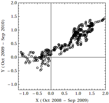
Figure 2. (a) Region of the parameter space (α,β,C)∈ℝ3(\alpha,\beta,C)\in\mathbb{R}^{3} where our proposed estimator y¯α,β\bar{y}_{\alpha,\beta} has lower MSE than the traditional estimators. (b) Scatterplot of study and auxiliary variables for the groundwater data studied in Section 6.

5. Unbiased AOE

Combining (4) and (8), we can calculate the parameters α\alpha and β\beta where our proposed estimator becomes – at least up to first approximation – an unbiased AOE. We obtain a line with

β=12andC=0,\beta=\frac{1}{2}\quad\text{and}\quad C=0,

(recall that on this line our estimator always reduces to the sample mean estimator) or a “curve” (α∗​(C),β∗​(C),C)∈ℝ(\alpha^{*}(C),\beta^{*}(C),C)\in\mathbb{R} in the parameter space with

(14) α∗​(C)=12​(1±C2​C−1)andβ∗​(C)=12​(1±C⁡(2​C−1)).\alpha^{*}(C)=\frac{1}{2}\left(1\pm\sqrt{\frac{C}{2C-1}}\right)\quad\text{and}\quad\beta^{*}(C)=\frac{1}{2}\left(1\pm\sqrt{C(2C-1)}\right).

We note that the parametric “curve” in (14) is only defined for C≤0C\leq 0 or C>12C>\frac{1}{2} – in fact, this parametric “curve” is three hyperbolas. The surface of “biasfree estimator parameters” in Fig. 1 (a) and the surface of “AOE parameters” in Fig. 1 (b) only intersect in these three hyperbolas and the line β=12\beta=\frac{1}{2} and C=0C=0. In the region 0<C≤120<C\leq\frac{1}{2} of the parameter space (α,β,C)∈ℝ3(\alpha,\beta,C)\in\mathbb{R}^{3}, we have the common situation where minimising MSE comes with a trade-off in bias. The curves of intersection are included in Fig. 1. Explicitly, our proposed estimator using the values in (14) is given by

(15) y¯∗​(C)=y¯α∗​(C),β∗​(C)=2​(C+1)​X¯2−2​(C−1)​x¯2+(2​C2−C−1)​(X¯−x¯)24​X¯​x¯−(2​C2−C−1)​(X¯−x¯)2​y¯.\bar{y}^{*}(C)=\bar{y}_{\alpha^{*}(C),\beta^{*}(C)}=\\ \frac{2\,(C+1)\,\bar{X}^{2}-2\,(C-1)\,\bar{x}^{2}+\left(2\,C^{2}-C-1\right)\,\left(\bar{X}-\bar{x}\right)^{2}}{4\,\bar{X}\,\bar{x}-\left(2\,C^{2}-C-1\right)\,\left(\bar{X}-\bar{x}\right)^{2}}\,\bar{y}.

At first it might seem surprising that this estimator y¯∗​(C)\bar{y}^{*}(C) is also defined in33 3 The denominator vanishes if C=14​(1±9​(X¯−x¯)2+32​X¯​x¯X¯−x¯)C=\frac{1}{4}\left(1\pm\frac{\sqrt{9\,(\bar{X}-\bar{x})^{2}+32\,\bar{X}\,\bar{x}}}{\bar{X}-\bar{x}}\right). the region 0<C≤120<C\leq\frac{1}{2}. However, one can also let the parameters (α,β)(\alpha,\beta) in the definition of our proposed estimator y¯α,β\bar{y}_{\alpha,\beta} in (1) be complex numbers – but such that we still get a real estimator. One can check that α∗​(C)\alpha^{*}(C) and β∗​(C)\beta^{*}(C) in (14) for 0<C<120<C<\frac{1}{2} have this property.

Furthermore, we can check that the first degree of approximation of the bias and MSE of y¯∗​(C)\bar{y}^{*}(C) are given by

𝔹1​(y¯∗​(C))=0andMSE1⁡(y¯∗​(C))=1−fn​SY2​(1−r2)\mathbb{B}_{1}\left(\bar{y}^{*}(C)\right)=0\qquad\text{and}\qquad\operatorname{MSE}_{1}\left(\bar{y}^{*}(C)\right)=\frac{1-f}{n}S_{Y}^{2}\left(1-r^{2}\right)

(compare (3) and (9)). Thus, the estimator y¯∗​(C)\bar{y}^{*}(C) of (15) is an unbiased AOE.

One might also ask whether inside 0<C≤120<C\leq\frac{1}{2} there is a choice of real parameters (α,β)∈ℝ2(\alpha,\beta)\in\mathbb{R}^{2} such that we get an AOE with small bias. Using (8) in (3), we get the first degree approximation of the bias of an AOE

𝔹1​(y¯α,β(o))=1−fn​CX2​Y¯​12​[C⁡(1−2​C)+(1−2​β)2].\mathbb{B}_{1}\left(\bar{y}^{(o)}_{\alpha,\beta}\right)=\frac{1-f}{n}C_{X}^{2}\bar{Y}\,\frac{1}{2}\left[C\left(1-2\,C\right)+(1-2\beta)^{2}\right].

From this expression (and the constraint (8)) it is clear that the bias can only be made zero if C≤0C\leq 0 or C≥12C\geq\frac{1}{2}. Otherwise, there is always a positive contribution coming from the term C⁡(1−2​C)C(1-2C) that does not vanish no matter what we choose for β∈ℝ\beta\in\mathbb{R}. In fact, it looks as if the choice β=12\beta=\frac{1}{2} always yields the least possible bias, however two remarks are in order here: Firstly, given (8) and unless C=0C=0, we can only let β\beta be close to 12\frac{1}{2} and choose α\alpha accordingly (the absolute value |α||\alpha| is then large). Secondly, we already noted that y¯α,12=y¯\bar{y}_{\alpha,\frac{1}{2}}=\bar{y}, and the MSE for the sample mean estimator is 1−fn​SY2\frac{1-f}{n}S^{2}_{Y}, not 1−fn​SY2​(1−r2)\frac{1-f}{n}S^{2}_{Y}(1-r^{2}) as for an AOE. We have arrived here at a point where the first degree approximation to bias and MSE breaks down. To find a choice of real parameters for given CC with minimal MSE and least bias, higher degrees of approximation would have to be considered.

6. Application and Conclusion

Using data taken from the Department of the Interior, United States Geological Survey (USGS) [9], site number 02290829501 (located in Florida), a comparison of our proposed estimator y¯α,β\bar{y}_{\alpha,\beta} to the traditional estimators was carried out. The study variables (denoted by YY) are taken to be the maximum daily values (in feet) of groundwater at the site for the period October 2009 to September 2010. The auxiliary variables (denoted XX) are taken as the maximum daily values (in feet) of groundwater for the period October 2008 to September 2009. Our goal is to estimate the true average maximum daily groundwater Y¯\bar{Y} for the period October 2009 to September 2010.

The questions we ask are: How many units of groundwater must be taken from the population YY to estimate the population mean Y¯\bar{Y} within d=10%d=10\% at a 90%90\% confidence level (α=0.10)(\alpha=0.10)? And how well do the estimators perform given this data set with auxiliary information for the calculated sample size nn?

Using the entire data set, we calculate the following statistics: Y¯≈0.5832\bar{Y}\approx 0.5832, X¯≈0.6277\bar{X}\approx 0.6277, SY≈0.4480S_{Y}\approx 0.4480, SX≈0.7222S_{X}\approx 0.7222, r≈0.9125r\approx 0.9125, CY≈0.7681C_{Y}\approx 0.7681, CX≈1.1504C_{X}\approx 1.1504 and C≈0.6092C\approx 0.6092. A scatterplot of the data set is shown in Fig. 2 (b), which adds emphasis to the positive measure of association between the study variable YY and the auxiliary variable XX.

One should note that the value of C≈0.6092C\approx 0.6092 lies in the interval (12,1)(\frac{1}{2},1), so we choose values of α\alpha and β\beta from Section 4.2. Indeed, we use (14) and choose β=β∗​(0.6092)≈0.3176\beta=\beta^{*}(0.6092)\approx 0.3176 and α=α∗​(0.6092)≈−0.3349\alpha=\alpha^{*}(0.6092)\approx-0.3349. Note that β=0.3176\beta=0.3176 yields (−0.8704)<α<0.200573(-0.8704)<\alpha<0.200573 in Section 4.2. Using the notation of Section 5, we also note that y¯−0.3349,0.3176=y¯∗​(0.6092)\bar{y}_{-0.3349,0.3176}=\bar{y}^{*}(0.6092).

6.1. Calculating the sample size nn

To estimate the population mean amount of groundwater recorded for the state of Florida from October 2009 to September 2010, a sample of size nn is drawn from the population of size N=365N=365 according to the simple random sampling without replacement [1]. A first approximation to this sample size needed is the (infinite population) value

n0=Zα22​σ2d2,n_{0}=\frac{Z_{\frac{\alpha}{2}}^{2}\sigma^{2}}{d^{2}},

where dd is the chosen margin of error from the estimate of Y¯\bar{Y}, and Zα2Z_{\frac{\alpha}{2}} is a standard normal variable with tail probability of α2\frac{\alpha}{2}. Accounting for the finite population size NN, we obtain the sample size

n=11n0+1N.n=\frac{1}{\frac{1}{n_{0}}+\frac{1}{N}}.

In general, the true value of σ2\sigma^{2} is unknown but can be estimated using its consistent estimator s2s^{2}. However, in our case σ2\sigma^{2} is calculated from the population and is given as SY2≈0.2006S_{Y}^{2}\approx 0.2006. Therefore, with α=0.10\alpha=0.10, d=10%​ of ​Y¯d=10\%\text{ of }\bar{Y} (i.e., d≈0.0583d\approx 0.0583) and Z0.05≈1.6449Z_{0.05}\approx 1.6449, the sample size can be calculated as n0≈(1.6449)2⋅0.2006(0.0583)2≈159.59n_{0}\approx\frac{(1.6449)^{2}\cdot 0.2006}{(0.0583)^{2}}\approx 159.59, rounding up gives n0=160n_{0}=160. Therefore, we get n≈11160+1365≈111.23n\approx\frac{1}{\frac{1}{160}+\frac{1}{365}}\approx 111.23, and thus take n=112n=112.

6.2. Relative efficiencies

Table 1 shows the relative efficiencies of the traditional estimators (sample mean y¯\bar{y}, ratio y¯R\bar{y}_{R} and product y¯P\bar{y}_{P} estimators) and our proposed two parameter ratio-product-ratio estimator y¯α,β\bar{y}_{\alpha,\beta} for (α,β)=(−0.3349,0.3176)(\alpha,\beta)=(-0.3349,0.3176). We note that with this choice of parameters, the estimator is an (unbiased) AOE, namely y¯−0.3349,0.3176=y¯∗​(0.6092)\bar{y}_{-0.3349,0.3176}=\bar{y}^{*}(0.6092). The table shows that our two parameter ratio-product-ratio estimator dominates the traditional estimators in the sense that it has the highest efficiency.

We can also observe that in the computation of the relative efficiency, the specification of the sample size nn is not important since the finite population correction factor (1−fn)(\frac{1-f}{n}) cancels out (however, this would not be the case for higher degrees of approximation).

Table 1. Relative efficiencies comparisons.
MSE⁡(y¯)MSE⁡(y¯)\frac{\operatorname{MSE}(\bar{y})}{\operatorname{MSE}(\bar{y})} MSE⁡(y¯)MSE1⁡(y¯R)\frac{\operatorname{MSE}(\bar{y})}{\operatorname{MSE}_{1}(\bar{y}_{R})} MSE⁡(y¯)MSE1⁡(y¯P)\frac{\operatorname{MSE}(\bar{y})}{\operatorname{MSE}_{1}(\bar{y}_{P})} MSE⁡(y¯)MSE1⁡(y¯∗​(0.6092))\frac{\operatorname{MSE}(\bar{y})}{\operatorname{MSE}_{1}\left(\bar{y}^{*}(0.6092)\right)}
100%100\% 196.11%196.11\% 16.73%16.73\% 597.28%597.28\%

6.3. Constructing a 90%90\% confidence interval for Y¯\bar{Y} using y¯α,β{\bar{y}}_{\alpha,\beta}

Constructing a 90%90\% confidence interval, the following formulation can be used (similar formulae hold for all estimators discussed here), see [1]:

(y¯∗​(0.6092)±Z0.05​SY2n⋅N−nN−1).\left(\bar{y}^{*}(0.6092)\pm Z_{0.05}\sqrt{\frac{S^{2}_{Y}}{n}}\cdot\sqrt{\frac{N-n}{N-1}}\right).

The factor (N−n)/(N−1)\sqrt{(N-n)/(N-1)} is the finite population correction.

Of course, by the choice of the sample size n=112n=112, we get a margin of error of approximately 0.1⋅Y¯≈0.05830.1\cdot\bar{Y}\approx 0.0583 here; more precisely, the calculation using the above formula yields (y¯∗​(0.6092)±1.6449⋅0.0423⋅0.8337)=(y¯∗​(0.6092)±0.0580)\left(\bar{y}^{*}(0.6092)\pm 1.6449\cdot 0.0423\cdot 0.8337\right)=\left(\bar{y}^{*}(0.6092)\pm 0.0580\right).

6.4. Comparison of estimators

To compare the proposed estimator with the traditional ones, we selected 10 00010\,000 times a sample of size n=112n=112 and calculate the estimators from it. We note that there are (365112)≈2.5⋅1096\binom{365}{112}\approx 2.5\cdot 10^{96} possibilities to choose 112112 data points out of a total 365365 without replacement.

In Table 2 we show the relative position of the estimators with respect to the population mean Y¯\bar{Y}. In the 10 00010\,000 simulations, our proposed estimator outperformed the traditional estimators on 4 7014\,701 occasions. The ratio estimator, the suggested estimator for this value of CC by [2], performs better than our proposed estimator 2 9782\,978 times (in these cases it is actually the best of the studied estimators; note that the ratio estimator is the worst 1 3491\,349 times).

In Table 3, we compare the estimators by looking at the following criteria: The coverage probability is the proportion of the 90%90\% confidence interval covering the population mean Y¯\bar{Y}; as expected, the usual mean sample estimator yields around 90%90\%, while the ratio estimator and our proposed estimator yield much higher values – in this simulation, all intervals calculated from our proposed estimator cover Y¯\bar{Y}. For those 90%90\% confidence intervals that do not cover Y¯\bar{Y}, we check whether they lie to the left (negative bias) or to the right (positive bias) of Y¯\bar{Y}. We also state the statistical information lower and upper quartile and median, we get from the 10 00010\,000 simulations; directly below this we show violin plots for the estimators (the dashed line indicates the value Y¯\bar{Y}, the dotted lines indicate the 90%90\% confidence interval). In the violin plot, we see that the values obtained by our proposed estimators yield a narrow normal distribution around the true value (skewness is 0.00460.0046, kurtosis is 2.99262.9926), while the product estimator gives a spread-out distribution and the (traditionally preferred) ratio estimator gives a skewed distribution (skewness is 0.52300.5230, kurtosis is 3.42533.4253). Finally, we compare the values of the MSEs; the experimental values obtained agree with the theoretical values listed in Table 1.

We infer that our proposed estimator is more efficient and robust than the traditional sample mean, ratio and product estimators.

Table 2. Comparison of the estimators according to the absolute deviation from the population mean Y¯\bar{Y} (in 10 00010\,000 simulations).
position counts
|y¯∗​(0.6092)−Y¯|\left|\bar{y}^{*}(0.6092)-\bar{Y}\right| << |y¯R−Y¯|\left|\bar{y}_{R}-\bar{Y}\right| << |y¯−Y¯|\left|\bar{y}-\bar{Y}\right| << |y¯P−Y¯|\left|\bar{y}_{P}-\bar{Y}\right| 3 173
|y¯R−Y¯|\left|\bar{y}_{R}-\bar{Y}\right| << |y¯∗​(0.6092)−Y¯|\left|\bar{y}^{*}(0.6092)-\bar{Y}\right| << |y¯−Y¯|\left|\bar{y}-\bar{Y}\right| << |y¯P−Y¯|\left|\bar{y}_{P}-\bar{Y}\right| 2 978
|y¯∗​(0.6092)−Y¯|\left|\bar{y}^{*}(0.6092)-\bar{Y}\right| << |y¯−Y¯|\left|\bar{y}-\bar{Y}\right| << |y¯R−Y¯|\left|\bar{y}_{R}-\bar{Y}\right| << |y¯P−Y¯|\left|\bar{y}_{P}-\bar{Y}\right| 1 528
|y¯−Y¯|\left|\bar{y}-\bar{Y}\right| << |y¯∗​(0.6092)−Y¯|\left|\bar{y}^{*}(0.6092)-\bar{Y}\right| << |y¯R−Y¯|\left|\bar{y}_{R}-\bar{Y}\right| << |y¯P−Y¯|\left|\bar{y}_{P}-\bar{Y}\right| 972
|y¯P−Y¯|\left|\bar{y}_{P}-\bar{Y}\right| << |y¯−Y¯|\left|\bar{y}-\bar{Y}\right| << |y¯∗​(0.6092)−Y¯|\left|\bar{y}^{*}(0.6092)-\bar{Y}\right| << |y¯R−Y¯|\left|\bar{y}_{R}-\bar{Y}\right| 766
|y¯−Y¯|\left|\bar{y}-\bar{Y}\right| << |y¯∗​(0.6092)−Y¯|\left|\bar{y}^{*}(0.6092)-\bar{Y}\right| << |y¯P−Y¯|\left|\bar{y}_{P}-\bar{Y}\right| << |y¯R−Y¯|\left|\bar{y}_{R}-\bar{Y}\right| 308
|y¯−Y¯|\left|\bar{y}-\bar{Y}\right| << |y¯P−Y¯|\left|\bar{y}_{P}-\bar{Y}\right| << |y¯∗​(0.6092)−Y¯|\left|\bar{y}^{*}(0.6092)-\bar{Y}\right| << |y¯R−Y¯|\left|\bar{y}_{R}-\bar{Y}\right| 275
Table 3. Comparison of the estimators in 10 00010\,000 simulations. See text for details.
estimator coverage neg. bias pos. bias lo. quart. median up. quart.
y¯\bar{y} 89.86%89.86\% 5.14%5.14\% 5.00%5.00\% 0.55830.5583 0.58200.5820 0.60620.6062
y¯R\bar{y}_{R} 97.01%97.01\% 0.12%0.12\% 2.87%2.87\% 0.56700.5670 0.58310.5831 0.60170.6017
y¯P\bar{y}_{P} 49.59%49.59\% 25.44%25.44\% 24.97%24.97\% 0.52400.5240 0.58090.5809 0.64100.6410
y¯∗​(0.6092)\bar{y}^{*}(0.6092) 100.00%100.00\% 0.00%0.00\% 0.00%0.00\% 0.57320.5732 0.58290.5829 0.59280.5928

estimator MSE MSE⁡(y¯)MSE⁡(est)\frac{\operatorname{MSE}(\bar{y})}{\operatorname{MSE}(\text{est})}
y¯\bar{y} 0.001270.00127 100%100\%
y¯R\bar{y}_{R} 0.000680.00068 186.68%186.68\%
y¯P\bar{y}_{P} 0.007550.00755 16.79%16.79\%
y¯∗​(0.6092)\bar{y}^{*}(0.6092) 0.000210.00021 598.93%598.93\%
[Uncaptioned image]

6.5. Outlook

Several authors have proposed efficient estimators using auxiliary information. For example, Srivastava and Reddy [8, 4] consider a generalisation to the product and ratio estimator given by y¯(k)=y¯​(x¯/X¯)k\bar{y}^{(k)}=\bar{y}\left({\bar{x}}/{\bar{X}}\right)^{k}; Reddy [4] also introduces the estimator y¯k=y¯​X¯/(X¯+k⁡(x¯−X¯))\bar{y}_{k}={\bar{y}\,\bar{X}}/\left({\bar{X}+k\,(\bar{x}-\bar{X})}\right); in Sahai et al. [5] the estimator y¯k​t=y¯​(2−(x¯/X¯)k)\bar{y}_{k\,t}=\bar{y}\,\left(2-(\bar{x}/\bar{X})^{k}\right) (where “t” stands for “transformed”) is considered; and Singh et al. [7] introduce a certain class of “ratio-product” estimators given by y¯R​P​(k)=y¯​(k⋅(X¯/x¯)+(1−k)⋅(x¯/X¯))\bar{y}_{RP}(k)=\bar{y}\left(k\cdot(\bar{X}/\bar{x})+(1-k)\cdot(\bar{x}/\bar{X})\right). Choosing appropriate parameters kk for these estimators and calculating the first degree approximation of the MSE, one can show that

MSE1⁡(y¯(−C))=MSE1⁡(y¯C)=MSE1⁡(y¯C​t)=MSE1⁡(y¯R​P​(C+12))=1−fn​SY2​(1−r2).\operatorname{MSE}_{1}\left(\bar{y}^{(-C)}\right)=\operatorname{MSE}_{1}\left(\bar{y}_{C}\right)=\operatorname{MSE}_{1}\left(\bar{y}_{C\,t}\right)=\operatorname{MSE}_{1}\left(\bar{y}_{RP}({\scriptstyle\frac{C+1}{2}})\right)\\ =\frac{1-f}{n}S_{Y}^{2}\left(1-r^{2}\right).

Thus, these estimators and our proposed estimator (see (9)) are equally efficient up to the first degree of approximation. Indeed, all these estimators give similar results as our proposed estimator in the above application, see Table 4. Comparing the first degree of approximation of the bias (doing calculations as in Section 2) reveals why our unbiased AOE y¯∗​(C)\bar{y}^{*}(C) and Reddy’s y¯C\bar{y}_{C} behave similar – they are both unbiased AOEs:

𝔹(y¯)=𝔹1(y¯∗(C))=𝔹1(y¯C)=0,𝔹1(y¯R)=1−fn(1−C)C2Xy¯,𝔹1(y¯P)=1−fnCC2Xy¯,𝔹1(y¯(−C))=1−fnC⁡(1−C)2C2Xy¯,𝔹1(y¯C​t)=1−fnC⁡(1−3​C)2C2Xy¯,𝔹1(y¯R​P(C+12))=1−fn(1+2​C)​(1−C)2C2Xy¯.\mathbb{B}(\bar{y})=\mathbb{B}_{1}\left(\bar{y}^{*}(C)\right)=\mathbb{B}_{1}\left(\bar{y}_{C}\right)=0,\quad\mathbb{B}_{1}\left(\bar{y}_{R}\right)=\frac{1-f}{n}(1-C)C^{2}_{X}\bar{y},\\ \mathbb{B}_{1}\left(\bar{y}_{P}\right)=\frac{1-f}{n}CC^{2}_{X}\bar{y},\quad\mathbb{B}_{1}\left(\bar{y}^{(-C)}\right)=\frac{1-f}{n}\frac{C(1-C)}{2}C^{2}_{X}\bar{y},\\ \mathbb{B}_{1}\left(\bar{y}_{C\,t}\right)=\frac{1-f}{n}\frac{C(1-3\,C)}{2}C^{2}_{X}\bar{y},\ \mathbb{B}_{1}\left(\bar{y}_{RP}({\scriptstyle\frac{C+1}{2}})\right)=\frac{1-f}{n}\frac{(1+2C)(1-C)}{2}C^{2}_{X}\bar{y}.

(With C=0.6092C=0.6092, only y¯C​t\bar{y}_{C\,t} is negatively biased, compare the quartiles and the box plot in Table 4). For our proposed estimator y¯α,β\bar{y}_{\alpha,\beta}, we are able to use the two parameters α\alpha and β\beta to obtain an estimator y¯∗​(C)\bar{y}^{*}(C) that is up to first degree of approximation both unbiased and has minimal MSE. A thorough comparison of these estimators involving higher degrees of approximation of MSE and bias as well as accompanying simulations might be desirable, e.g., to find the estimator that behaves well if the coefficient of correlation CC is not known exactly.

Table 4. Comparison of AOEs in 10 00010\,000 simulations. See text for details.
estimator coverage neg. bias pos. bias lo. quart. median up. quart.
y¯∗​(0.6092)\bar{y}^{*}(0.6092) 100%100\% 0%0\% 0%0\% 0.57320.5732 0.58290.5829 0.59280.5928
y¯(−0.6092)\bar{y}^{(-0.6092)} 100%100\% 0%0\% 0%0\% 0.57380.5738 0.58350.5835 0.59350.5935
y¯0.6092\bar{y}_{0.6092} 100%100\% 0%0\% 0%0\% 0.57320.5732 0.58290.5829 0.59280.5928
y¯0.6092​t\bar{y}_{0.6092\,t} 100%100\% 0%0\% 0%0\% 0.57190.5719 0.58160.5816 0.59150.5915
y¯R​P​(0.8046)\bar{y}_{RP}(0.8046) 99.99%99.99\% 0%0\% 0.01%0.01\% 0.57490.5749 0.58500.5850 0.59530.5953

estimator MSE MSE⁡(y¯)MSE⁡(est)\frac{\operatorname{MSE}(\bar{y})}{\operatorname{MSE}(\text{est})}
y¯∗​(0.6092)\bar{y}^{*}(0.6092) 0.0002120.000212 598.93%598.93\%
y¯(−0.6092)\bar{y}^{(-0.6092)} 0.0002140.000214 593.91%593.91\%
y¯0.6092\bar{y}_{0.6092} 0.0002120.000212 598.92%598.92\%
y¯0.6092​t\bar{y}_{0.6092\,t} 0.0002150.000215 590.51%590.51\%
y¯R​P​(0.8046)\bar{y}_{RP}(0.8046) 0.0002280.000228 555.09%555.09\%
[Uncaptioned image]

References

  • [1] W.G. Cochran, Sampling Technique, 3rd ed., Wiley, New York, 1977, \htmladdnormallinkMR0474575http://www.ams.org/mathscinet-getitem?mr=0474575.
  • [2] M.N. Murthy, Product method of estimation, Sankhyā A26(1): 69–74 (1964), \htmladdnormallinkMR0193706http://www.ams.org/mathscinet-getitem?mr=0193706. Available at \htmladdnormallinkhttp://www.jstor.org/stable/25049308http://www.jstor.org/stable/25049308.
  • [3] S.K. Ray and A. Sahai, Efficient families of ratio and product-type estimators, Biometrika 67(1): 211–215 (1980), \htmladdnormallinkMR0570521http://www.ams.org/mathscinet-getitem?mr=0570521. Available at \htmladdnormallinkhttp://www.jstor.org/stable/2335336http://www.jstor.org/stable/2335336.
  • [4] V.N. Reddy, On ratio and product methods of estimation, Sankhyā B35(3): 307–316 (1973), \htmladdnormallinkMR0405693http://www.ams.org/mathscinet-getitem?mr=0405693. Available at \htmladdnormallinkhttp://www.jstor.org/stable/25051845http://www.jstor.org/stable/25051845.
  • [5] A. Sahai and S.K. Ray, An efficient estimator using auxiliary information, Metrika 27(1): 271–275 (1980), \htmladdnormallinkMR0598736http://www.ams.org/mathscinet-getitem?mr=0598736. Available at \htmladdnormallinkhttp://dx.doi.org/10.1007/BF01893605http://dx.doi.org/10.1007/BF01893605.
  • [6] A. Sahai and A. Sahai, On efficient use of auxiliary information, J. Stat. Plann. Inference 12: 203–212 (1985), \htmladdnormallinkMR0807865http://www.ams.org/mathscinet-getitem?mr=0807865. Available at \htmladdnormallinkhttp://dx.doi.org/10.1016/0378-3758(85)90070-9http://dx.doi.org/10.1016/0378-3758(85)90070-9.
  • [7] H.P. Singh and M. Ruiz Espejo, On linear regression and ratio-product estimation of a finite population mean, J. R. Stat. Soc. D52(1): 59–67 (2003), \htmladdnormallinkMR1973882http://www.ams.org/mathscinet-getitem?mr=1973882. Available at \htmladdnormallinkhttp://www.jstor.org/stable/4128169http://www.jstor.org/stable/4128169.
  • [8] S.K. Srivastava, An estimator using auxiliary information in sample surveys, Calcutta Stat. Assoc. Bull. 16(62–63): 121–132 (1967), \htmladdnormallinkMR0220428http://www.ams.org/mathscinet-getitem?mr=0220428.
  • [9] United States Geology Survey, Water resources of the United States — annual water data report, accessed on 17 December 2011 at \htmladdnormallinkhttp://wdr.water.usgs.gov/http://wdr.water.usgs.gov/.