Random billiards with wall temperature and associated Markov chains
Abstract
By a random billiard we mean a billiard system in which the standard specular reflection rule is replaced with a Markov transition probabilities operator that, at each collision of the billiard particle with the boundary of the billiard domain, gives the probability distribution of the post-collision velocity for a given pre-collision velocity. A random billiard with microstructure, or RBM for short, is a random billiard for which is derived from a choice of geometric/mechanical structure on the boundary of the billiard domain. Such random billiards provide simple and explicit mechanical models of particle-surface interaction that can incorporate thermal effects and permit a detailed study of thermostatic action from the perspective of the standard theory of Markov chains on general state spaces.
The main focus of the present paper is on the operator itself and how it relates to the mechanical and geometric features of the microstructure, such as mass ratios, curvatures, and potentials. The main results are as follows: (1) we characterize the stationary probabilities (equilibrium states) of and show how standard equilibrium distributions studied in classical statistical mechanics, such as the Maxwell-Boltzmann distribution and the Knudsen cosine law, arise naturally as generalized invariant billiard measures; (2) we obtain some basic functional theoretic properties of . Under very general conditions, we show that is a self-adjoint operator of norm on an appropriate Hilbert space. In a simple but illustrative example, we show that is a compact (Hilbert-Schmidt) operator. This leads to the issue of relating the spectrum of eigenvalues of to the geometric/mechanical features of the billiard microstructure; (3) we explore the latter issue both analytically and numerically in a few representative examples; (4) we present a general algorithm for simulating these Markov chains based on a geometric description of the invariant volumes of classical statistical mechanics. Our description of these volumes may also have independent interest.
1 Introduction
This extended introduction contains some definitions and an overview of the main results. Additional results and refinements are discussed throughout the text.
1.1 Physical motivation
Consider the idealized and somewhat fanciful billiard system shown in Figure 1. At a “macroscopic scale” it consists of a point particle, henceforth called the molecule, and a billiard table having piecewise smooth wall (only a small part of which is shown). At a “microscopic scale,” both the wall and the molecule may reveal further geometric and mechanical structure that can affect the outcome of a collision. Thus collisions are not necessarily specular; to specify the outcome of a collision it is necessary to consider the interaction between molecule and wall at this finer scale. We suppose that the wall system is kept at a constant statistical state, say, a canonical ensemble distribution with a given temperature, and wish to follow the evolution of the statistical state of the molecule. The outcome of a molecule-wall collision event is then shown to be described by a time-independent transition probabilities operator , to be defined later as an operator on an space over the set of pure states of the molecule. This operator, which as we will see is canonically defined by the mechanical/geometric features of the wall and molecule microstructure and the constant statistical state of the wall, replaces the mirror-reflection map of an ordinary billiard. We call a system of this kind a random billiard with microstructure, or RBM.

Discrete-time Markov chains associated to are interpreted as random states of the molecule immediately after each collision, starting from some initial probability distribution, at least for simple shapes of the the billiard domain such as cylinders or balls. Besides determining the equilibrium states of the molecule as the stationary (i.e., -invariant) probability distributions for the Markov chain, the operator contains information about rates of decay of correlations and spectral data, which can in principle be used to derive transport coefficients such as the diffusion constant of a gas of non-interacting molecules moving inside a “billiard channel.” (See Figure 3.)
Here we develop some of these ideas in detail, focusing on the billiard-Markov operator and its relationship with the microstructure. The main results of the paper are concerned with defining for any given Newtonian molecule-wall system, deriving its basic functional analytic properties, describing stationary probability distributions, and illustrating with concrete examples some of the spectral properties of P.
There are several sources of motivations for this work, some purely mathematical and others more applied. On the purely mathematical side, we seek to have interesting and well-motivated classes of Markov chains that can be used to investigate issues of general interest in probability theory, such as spectral gap, mixing times, central limit theorems, etc. The statistical mechanics perspective in combination with very simple mechanical systems provides a great variety of examples. We also believe that generalized billiard systems of the kind we are considering may provide fruitful examples of random (often hyperbolic) dynamical systems with singularities, i.e., random counterparts of the widely studied chaotic billiards, for which [3] is a recommended reference. On the more applied side, processes of the kind we are studying here may be useful in kinetic theory of gases as suggested, for example, in [7] in the context of Knudsen diffusion studies. In the context of the theory of Boltzmann equations, operators such as our may serve to specify boundary conditions for gas-wall systems. (See, for example, [2] for the context in the theory of Boltzmann equations in which related operators, but not derived from any explicit microscopic interaction model like ours, arise.) Our random collision operators provide very natural and simple Newtonian models for the interaction of a molecule with a heat bath that can be used to study thermostatic action fairly explicitly and often analytically from the perspective of the general theory of Markov chains.
1.2 The surface-scattering set-up
The main definitions pertaining to the billiard microstructure are as follows. Let be a smooth manifold whose points represent the configurations of a mechanical system. The system consists of two interacting subsystems: the wall and the molecule. A motion in describes a molecule-wall collision event in which the molecule comes close to the the wall surface, scatters off of it, and moves away. Let smooth Riemannian manifolds and be the configuration spaces of the wall and the molecule subsystems; to capture the idea that there is a direction towards which the (center of mass of) the molecule approaches the plane of the wall, and that the microstructure on the wall is periodic, we assume that factors as a Riemannian product
where is the manifold of molecular configurations under the assumption that the center of mass is at a fixed position. For the examples of interest, .
In the example of Figure 1, is simply an interval , representing the range of positions of the wall-bound mass attached to the spring. The Riemannian metric on is derived from the kinetic energy of the wall-bound mass. The manifold may be written as , specifying the spatial orientation (or angle of rotation) of the hollowed little disc and the position of the vibrating mass in its interior. The Riemannian metric is, again, derived from the kinetic energy of the molecule system, so metric coefficients are given by the values of masses and moments of inertia. The plane of the wall is aligned with the factor and the direction of approach of the molecule is the factor in the product. We disregard the possible (“macroscopic”) curvature of the billiard table boundary—the interaction is imagined to happen at a length scale in which boundary curvature cannot be discerned.
Back to the general case, the combined wall-molecule system is represented by with a Riemannian metric and a potential function such that (1) the two subsystems are non-interacting when they are sufficiently far apart (more details below) and, (2) for each value of the total energy , where for , the subset of the level set consisting of states at which the subsystems are a bounded distance from each other has finite volume with respect to the invariant volume form , whose definition is recalled later.
To explain assumption (1), we assume the existence of a smooth function , interpreted as the distance in Euclidian space from the center of mass of the molecule to some reference position on the wall. For each real number define and , and denote by and the projections onto and , respectively. Then we suppose that there exists an , which can be taken with no loss of generality to be less than , such that, for all ,
- i.
the set is isometric to, and will be identified with,
- ii.
there are smooth functions and such that
- iii.
for each value of the energy function the level set has finite volume relative to ;
- iv.
the system is essentially dynamically complete, in the following sense: Any smooth curve that satisfies Newton’s equation (with acceleration defined in terms of the Levi-Civita connection)
can be extended indefinitely in the interior of , until it reaches the boundary; whenever intersects the boundary transversely at a regular point , it can be extended further back into the interior along the unique solution curve with initial state , where and is the standard reflection map.
In the example of Figure 2, is the two-point set labeling the two sheets of above a certain distance from the handles. The manifold consists of a single point and the potential function is constant. We give , say, the Riemannian metric induced from Euclidean -space. More representative examples, in which is non-trivial will be shown later.

As already noted, the various manifolds above may have boundary. Boundary points represent collision configurations. It is necessary to accept manifolds whose boundaries may not be smooth. For concreteness, we adopt here the class of manifolds with corners (see [10]), which is general enough to provide plenty of meaningful examples. In particular, contains a set , the singular boundary, the complement of which is a smooth manifold with boundary in the ordinary sense of being modeled on open subsets of the upper half space. This complement is the union of the interior set , and the (regular) boundary . Moreover, is contained in the closure of , it is nowhere dense in this closure and has measure in . Since we are mainly interested in probabilistic questions, it is typically safe to ignore the singular boundary set.
If is a regular boundary point of and is a unit vector perpendicular to the boundary at , we assume that a motion in is extended after hitting the boundary at in such a way that the pre- and post-collision velocities and are related according to the standard linear (reflection) map ; so “microscopic” collisions are specular. Being an isometry of the kinetic energy metric, this map leaves the energy function invariant.
Let be the level set in , i.e.,
and the restriction of to (more precisely, the pull-back of under the inclusion ). Informally, crossing amounts to entering the zone of interaction , though S itself lies in the product zone. The vectors in pointing into the zone of interaction form the subset . This is the set of incoming states. The set of outgoing states, , is similarly defined as the set of vectors in pointing out of the zone of interaction. Omitting, as we often do, the base point in when referring to a state in , then sends an element of to an element of . Let , where is the half-space in . Then the incoming states decompose as a product
where and . We have chosen this particular decomposition so that the “observable” quantities of the molecule are grouped into the first factor and the quantities to be chosen probabilistically are grouped into the second and third factors.
A collision event is defined by an application of the map , which gives the return state from an initial state in , obtained by integrating the equations of motion. Under our general assumptions this map is defined on almost all initial states by Poincaré recurrence, and for many systems of interest it can be shown that is smooth on a dense open set of full measure. We make this almost everywhere smoothness a standing assumption. For simplicity, we indicate the domain of simply by , ignoring the fact that it is really defined on an open dense subset of full measure. It is convenient to redefine by composing it with the reflection map , so that becomes a self-map of . Thus we add to the above list of assumptions:
- v.
the return map is smooth on an open dense subset of of full measure.
1.3 The Markov operator
Let be any given probability measure on . The physically most natural and interesting choice for corresponds to taking the product of the uniform distribution on and the Gibbs canonical distribution on with parameter , whose definition is recalled later. The choice of measure fixes the statistical state of the wall system. The collection of possible states of the molecule system is the space of Borel probability measures on . We now define the map
that associates to each statistical state the new state . Notations and general explanations are further provided in Section 2. The interpretation is that, to obtain the return statistical state of the molecule, we take its present state , form the combined state of the system, let it evolve under , thus yielding , and finally project the outcome back to under the natural projection . The asterisk indicates the push-forward operation on measures.
Consider again the system of Figure 2 as an example. In that case is trivial (a single point) and is identified with , where is the half-plane in . It does not make sense in this case to consider a Gibbs canonical distribution—a natural measure here is the uniform probability distribution on . Since in this example the speed of the particle does not change, we consider not the full but a level set for the energy (say, only states with unit velocity). So we let , which parametrizes the sheet number () and the angle of the incoming trajectory relative to the normal to the wall plane.
Writing for a point in , we can define by first indicating how it acts on, say, essentially bounded functions on and then defining its action on by duality, , where indicates the integral of with respect to . Thus if is a bounded function on , and is the state of return to under for , then from the general definition we have,
When the (macroscopic) billiard table is a channel as shown in Figure 3, iterates of give the post-collision states of a random flight of the molecule (say, in a gas of non-interacting molecules) inside the channel.

Diffusion approximation of the random flight and the dependence of the diffusion constant on the spectrum of are issues of particular interest, which will be investigated in another paper dedicated to central limit theorems for and related topics.
1.4 Overview of the main results
The starting point of our analysis is a determination of the stationary probability measures of . Recall that a probability measure is said to be stationary for if . We consider two possibilities: (1) the space reduces to a point, in which case the wall is regarded as a rigid, unmoving body that does not exchange energy with the billiard particle in a collision. Note that, in this case, the billiard chamber might still have a non-trivial structure, but it does not contain moving parts. In this case, the measure that enters in the definition of is taken to be the normalized Lebesgue measure on ; (2) the space has dimension at least one. This means that the wall system has moving parts and energy can be transferred between wall and molecule in a collision. In this case we assume for the purposes of the next theorem that is the product of the normalized Lebesgue measure on and the Gibbs canonical measure on the phase space with a fixed parameter . The latter can be written as follows (a fuller discussion of invariant measures is given in the last section of the paper):
| (1.1) |
where is the energy function on , is the invariant (Liouville) volume form on energy level sets in derived from the symplectic form on this space, and the vertical bars indicate the associated measure. The denominator is a normalization factor.
We consider similar measures on More precisely, in case (1) we fix a value of the energy function of the molecule, which remains constant throughout the process, and consider the microcanonical measure for this value, given by
| (1.2) |
where is the hypersurface of separation between the product zone and the zone of interaction previously described, is the invariant volume form on the part of the level set above and the denominator is a normalizing factor. In case (2) we define
| (1.3) |
A description of these measures better suited for applications will be given shortly. In the special case when reduces to a point, so that , these measures are as follows: in case (1) we may choose so that the molecule state lies in the unit hemisphere in . Indicating by the standard volume form on the unit hemisphere and by the unit normal vector to , say, pointing into the zone of interaction, we have, up to a normalization constant ,
which we refer to as the Knudsen probability distribution; and in case (2)
where and are, respectively, the standard inner product and volume element in . This measure is the Maxwell-Boltzmann distribution at boundary points.
Theorem 1.
Let be the Markov operator associated to a probability measure on .
- 1.
In case (1) above, let be the normalized Lebesgue measure on . Then the microcanonical distribution 1.2 is a stationary probability for .
- 2.
In case (2) above, let be the product of the normalized Lebesgue measure on and the Gibbs canonical distribution on with temperature parameter . Then the Gibbs canonical distribution on given by 1.3, with the same parameter , is a stationary probability for .
In the particular case when the molecule reduces to a point, the stationary measures are, respectively, the Knudsen distribution in case (1) and the boundary Maxwell-Boltzmann distribution in case (2).
The proof of this theorem is given at the end of Subsection 5.4. The stationary probability is often (but not always) unique and one often obtains convergence of to the stationary state for any initial distribution . Thus the dynamic of a Markov chain derived from describes the process of relaxation of the molecule’s state toward thermal equilibrium with the wall. To understand this process in each particular situation it is necessary to study the operator in more detail; we do this later in the text for a few concrete examples.
The following definition is further elaborated in Section 2. We say that the molecule-wall system is symmetric if on the state space are defined two automorphisms and such that:
- i.
these maps preserve the natural measure on derived from the symplectic structure;
- ii.
they respect the product fibration and both induce the same map on ; that is,
- iii.
is time reversing: ; and commutes with : .
The existence of the map is typically assured by the time reversibility of Newtonian mechanics and the symmetry can often be obtained by a simple extension of the original system that does not affect its essential physical properties. (This is akin to defining an orientation double cover of a possibly non-oriented manifold.) The assumption of symmetry is thus a very weak one. These points are further discussed in Section 2 and in some of the specific examples studied later in the paper.
It is natural to consider the associated operator, still denoted , on the Hilbert space , where is one of the stationary probabilities obtained in Theorem 1. We are particularly interested in the spectral theory of . A first general observation in this direction is the following.
Theorem 2.
Let be the stationary measure of obtained in Theorem 1 and suppose that the system is symmetric. Then is a self-adjoint operator on of norm .
In particular, has real spectrum contained in . It is often the case (this will be proved for a simple but representative example later in this paper, and has been shown for special classes of in previous papers; see [6, 8]) that is a compact, integral operator (Hilbert-Schmidt). The eigenvalues of are then invariants of the system, depending in a canonical way on structural parameters like mass ratios, potential functions, curvatures, etc. The relationship between the spectrum of and these parameters is one of the central issues in this subject.
Of particular interest is the spectral gap of , defined as minus the spectral radius of the restriction of to the orthogonal complement to the constant functions. As is well-known (see, for example, [13]) the spectral gap can be used to estimate the exponential rate of convergence of to the stationary distribution in the total variation or the norm.
A perturbation approach to the spectrum of , which is valid when the molecule scattering is not far from specular, can be very fruitful. To make sense of this, first define
where dist is a distance function on , is an initial state, is the random variable representing the scattered state after one collision event, and is conditional expectation given the initial state . We call the second moment of scattering. Under the identification of and (see above), specular reflection corresponds to almost surely and small deviations from specularity correspond to small values of the second moment of scattering. We now defined the operator
which we refer to as the random billiard Laplacian (or the Markov Laplacian) of the system. The billiard Laplacian, for small values of often approximates a second order differential operator. In the examples studied, this will be seen to be a (densely defined) self-adjoint operator on the same Hilbert space on which is defined, whose eigenvalue problem amounts to a standard Sturm-Liouville equation.

In Section 3 we explore these ideas in detail with an example. The example consists of two point masses (see Figure 4) constrained to move along the half-line . Mass , with position coordinate , is restricted to move in the interval and , with position coordinate , can move freely on . The two masses collide elastically, and collides elastically with walls at and . The wall at is regarded as permeable to but not to . The random state of is taken to be the product of the uniform distribution over and a Gaussian probability with mean and variance for its velocity. Mass is the molecule and mass is part of the wall system. We refer to this as the two-masses system. To simplify notation and for other conveniences we rescale positions and velocities according to and , where . The main structural parameter of the system is the mass-ratio . We let represent the Markov operator with mass-ratio . Further details are explained in Section 3. We summarize in the next theorem some of the main conclusions obtained for the two-masses example. (Further refinements and numerical calculations are described in that section.)
Theorem 3 (Case study).
The following assertions hold for the two-masses system with :
- 1.
has a unique stationary distribution . Its density relative to Lebesgue measure on is given by
- 2.
For an arbitrary initial probability distribution , we have exponentially fast in the total variation norm.
- 3.
is a Hilbert-Schmidt operator.
- 4.
If is a function of class on , then the billiard Laplacian has the following limit
Equivalently, can be written in Sturm-Liouville form as which is a densely defined self-adjoint operator on .
Based on part 4 of the above theorem and a simple analysis of the corresponding Sturm-Liouville eigenvalue problem (the equation in part 4 is, after the change of coordinates , Laguerre’s equation), we can make an educated guess as to the asymptotic value, for small , of the spectral gap of : it is given by . Although we do not prove this here, we offer in Section 3 numerical evidence for its validity. This gives the following refinement of item 2 of Theorem 3:
is a positive constant and as the mass-ratio parameter approaches . (A general spectral perturbation study of our Markov operators with small moment of scattering based on comparison with Sturm-Liouville eigenvalue equations will be given in another paper.)
1.5 An algorithm for the Markov chain simulation
The map generating the deterministic discrete dynamical system involved in the definition of is essentially a kind of billiard map [3] in a very general setting. For applications of Theorem 1, particularly in numerical simulations of the Markov chains, we need a convenient expression for the corresponding invariant billiard measure and for the Gibbs distributions. We recall that the standard invariant billiard measure for planar billiards can be described as follows: If states of the billiard system are represented by coordinates , where is proportional to arclength measured from a reference point on the boundary of the billiard table (assuming that this boundary has finite length) and measures the angle that a unit velocity vector based at the point represented by makes with the inward pointing normal vector, then is the canonical invariant probability measure on the two-dimensional state space of the billiard system. See, for example, [3]. We wish to have a similar description of the invariant billiard measure on boundary components of general Riemannian manifolds in the presence of potential functions. Although this is something rather classical and possibly relatively well-known, we could not find it in the literature in a form that is convenient for our needs. It may thus be of some interest to highlight such an expression here. After doing this, we give at the end of this subsection the outline of an algorithm for generating Markov chains associated to general microstructures.
The next theorem is of some independent interest having to do with a representation of the standard volume measures of classical statistical mechanics. Our primary interest is to apply the theorem to a neighborhood of in the non-interaction zone of described above. But, in the interest of generality, the notation in this section is similar to, but independent of what was used above. In particular, we will reuse to mean any smooth Riemannian manifold with corners and any smooth potential function.
As always, we let the kinetic energy be defined by the Riemannian metric, , and consider the Hamiltonian flow on with standard energy function , where is the base-point projection. Let be the dimension of and an -dimensional submanifold of the boundary of . Let be the intersection of , defined just as in the more specialized setting of the molecule-wall systems, with the constant energy submanifold of . We assume that the return map is defined (in the a.e. sense described above); let be the unit normal vector field on pointing towards the interior of ; and for any given value define , where and
| (1.4) |
Extend to all of by setting on the complement of . Now let be an open set in on which is defined an orthonormal frame of vector fields ; let be the part of above , and let be the map such that
where is the unit sphere in . Then is a diffeomorphism and maps the unit sphere bijectively onto the fiber of above . If intersects or more generally , we assume that at any the vector is perpendicular to .
The Riemannian volume form on will be denoted by and that on by . Recall that the relationship between and is that , the interior multiplication of by the unit normal vector vector field on . Let be the Euclidean volume form on , which is obtained from the standard volume form on by interior multiplication with the unit radial vector field. In Section 5 we define the (microcanonical) invariant forms and on and , respectively, in terms of the symplectic form and prove the following.
Theorem 4 (Invariant volumes).
For any choice of orthonormal frame over an open set , and given the frame map defined above, the form satisfies
If is a neighborhood of a point in , we similarly have
where is the angle that makes with for . Apart from the unspecified signs, these expressions do not depend on the choice of local orthonormal frame.
The first volume form is invariant under the Hamiltonian flow, and the second is invariant under the return map to . We refer to the latter as the billiard volume form and to the former as the Liouville volume form. The Gibbs canonical distribution with temperature parameter is then the probability measure obtained from the volume form
on ; similarly the Gibbs volume form is defined on using the billiard volume form just introduced above. These volumes on and on are also invariant under the Hamiltonian flow and under , respectively. The probability measure on associated to the billiard volume form may also be called the Gibbs microcanonical distribution. Note how the probability of occupying a state of high potential energy in the microcanonical distribution depends on the potential function (thus on the position in ) due to the term .
Given the representation of the invariant volumes of Theorem 4, we can state the Markov chain algorithm as follows.
- MC1.
Start with a , representing the state of the molecule prior to a collision event;
- MC2.
Choose with probability density proportional to , representing the energy of the wall system;
- MC3.
Choose with probability density proportional to relative to the Riemannian volume (which defines uniform distribution), where is the dimension of ;
- MC4.
Choose a random vector over the unit sphere in with the uniform distribution;
- MC5.
Set the state of the wall prior to the collision event to ;
- MC6.
Use the combined state as the initial condition of the molecule-wall system prior to collision and let it evolve according to the deterministic equations of motion until the molecule leaves the zone of interaction; record the state of the molecule at this moment.
This procedure is illustrated in Subsection 4.2 with an example that is similar to that of Section 3 but now involving a non-constant potential function. Similarly interpreting Theorem 1, a (typically unique) stationary distribution for a Markov chain with transitions can be sampled from in the following way:
- SD1.
Choose with probability density proportional to ;
- SD2.
Choose in with probability density proportional to , where is now the dimension of the latter manifold;
- SD3.
Choose a random vector over the unit sphere in with probability density proportional to , where is the angle between the velocity of the molecule’s center of mass and the normal to the submanifold (which the molecule has to cross to enter the region of interaction);
- SD4.
Set the sample value of the equilibrium state of the molecule to be .
2 Random dynamical systems
In this section we derive a few general facts concerning random dynamical processes with the main goal of proving Theorem 2. A useful perspective informing this discussion is that our Markov chains arise from deterministic systems of which only partial information is accessible. The notation employed below is independent of that of the rest of the paper.
2.1 The Markov operator in general
Let denote a measured fibration, by which we simply mean a measurable map between Borel spaces together with a family of probability measures on fibers, so that for each . The family is measurable in the following sense: If is a Borel function then is Borel, where indicates the integral of with respect to . We refer to as the probability kernel of the fibration.
A random system on is specified by the data , where is a measured fibration with probability kernel , is the initial probability distribution on , and is a measurable map. We think of the map as the generator of a deterministic dynamical system on the state space . A point in represents a fully specified state of the system, of which the “observer” can only have partial knowledge represented by . (It is not assumed that maps fibers to fibers.)
From this we define a Markov chain with state space as follows. Let be a probability measure on representing the statistical state of the (observable part of the) system at a given moment. Then the state of the system at the next iteration is given by
The notation should be understood as follows. From and we define a probability measure on so that for any, say function
The push-forward operation on measures is defined by The result is an operator taking probability measures to probability measures, which we refer to as the Markov operator. When it is helpful to be more explicit we write, say, or , instead of .
The probability kernel is the family of transition probabilities of the Markov chain. In keeping with standard notation, we let act on measures (states) on the right, and on functions (observables) on the left. Thus is the function such that for all . It follows that
We say that is the disintegration of a probability measure on relative to a probability on if .
A probability measure on is invariant under if , and a probability measure on is stationary for the random system if .
Proposition 1.
Let be a -invariant probability measure on the total space of the random system and suppose that is the disintegration of with respect to . Then is a stationary probability measure on .
Proof.
This is immediate from the definitions:
We have used that . ∎
Let be a probability measure on and define the Hilbert space with inner product
Proposition 2.
Let be a random system, where is an isomorphism (thus it has a measurable inverse) of the measure space and is -invariant. Let be the associated Markov operator. Then , regarded as an operator on , has norm and its adjoint is .
Proof.
Jensen’s inequality implies
The integral on the right equals , by -invariance of . As is constant on fibers, this last integral is , showing that the norm of the operator is bounded by . Taking shows that the norm actually equals . To see that the adjoint equals the operator associated to the inverse map, simply observe the identity
which is due to -invariance of . ∎
2.2 Time reversibility and symmetry
Let be a -invariant random system, which means by definition that is a -invariant measure so, in particular, is stationary. We say that the system is time reversible if there is a measurable isomorphism respecting and , in the sense that it maps fibers to fibers and , and satisfies
Since respects , it induces a measure preserving isomorphism (for the measure ) such that We denote also by the induced composition operator on , so that . Notice that such is a unitary operator on . We call the time-reversing map of the system.
Proposition 3.
Let be a -invariant random system with time-reversing map , and its associated unitary operator on . Then
Proof.
A straightforward consequence of the definitions is that
from which we obtain
The last integral is now seen to be equal to by using the invariance of under and . ∎
We say that is an automorphism, or a symmetry of the random system if it is a measurable isomorphism commuting with that respects and . Thus covers a measure preserving isomorphism of , which we denote by .
Definition 1.
The -invariant, time reversible random system with time reversing map will be called symmetric if there exists an automorphism whose induced map on coincides with the map induced from .
Proposition 4.
Let be a symmetric (hence time-reversible and -invariant) random system. Then the Markov operator is self-adjoint. In particular, .
Proof.
Given Proposition 3, it is enough to verify that commutes with the operator . Keeping in mind that , , and that is -invariant, we obtain
This means that . The claim follows as is unitary. ∎
Corollary 1.
Let be a -invariant random system, where is an involution, i.e., equals the identity map on . Then the Markov operator is self-adjoint.
Proof.
Since , the identity map on is both a time reversing map and a symmetry of the system. ∎
The situation indicated in Corollary 1 essentially describes a general stationary Markov chain satisfying detailed balance. In that case, is the state space of the Markov chain, (or, more generally, a measurable equivalence relation on ), and is a probability measure on for each . For we take the (groupoid) inverse map . As a special case, we suppose that is countable and write in more standard notation and . Then the random system is symmetric as define above exactly when the Markov chain on with transition probabilities and stationary distribution satisfies the detailed balance condition for all .
2.3 Quotients
A minor technical issue to be mentioned later calls for a consideration of quotient random systems. Suppose that is a group of symmetries of the random system and that the action of on , as well as the induced action on , are nice in the sense that the quotient measurable spaces are countably separated. (See, for example, [14], where such actions are called smooth. In the situations of main concern to us, is a finite group acting by homeomorphisms of a metric space, in which case the condition holds.) Without further mention let the actions of be nice.
We denote the quotient system by , and the other associated notions, such as and , are similarly indicated with an over-bar. The quotient maps and will both be indicated by . These maps and measures are all defined in the most natural way. For example, is the transformation on such that , which exists since commutes with , , etc. Since leaves invariant, it is represented by unitary transformations of commuting with . So it makes sense to restrict to the closed subspace of -invariant vectors, which is isomorphic to the Hilbert space under the map that sends to . Thus we may identify the quotient Markov operator with the restriction of to the -invariant subspace.
We use these remarks later in situations where the initial system does not have any symmetries that would allow us to apply Proposition 4, but it can nevertheless be regarded as the quotient of another system having the necessary symmetry.
3 A case study: the two-masses system
In this section we prove Theorem 3 and further refinements, which are concerned with one simple but illustrative molecule-wall system. Other examples are described more briefly later in the next section.
3.1 Description of the example
Let represent the positions of two point masses restricted to move on the half-line , with respective masses and . Mass , called the bound mass, is restricted to move between and , and it reflects elastically upon hitting or , moving freely between these two values. Mass , called the free mass, moves freely on the interval , and collides elastically with when . There are no forces or interactions of any kind other than collisions. We are interested in the following “scattering experiment”: Mass starts at some place along the half-line with coordinate and speed , moving towards the origin. It eventually collides with , possibly several times, before reversing direction and leaving the “interval of interaction” . When it finally reaches again a point with coordinate , we register its new speed (now moving away from the origin). It is assumed that we can measure and exactly, but that the state of at the moment the incoming mass crosses the boundary is only known up to a probability distribution.

More specifically, we assume that, at that moment in time, is a random variable uniformly distributed over and that the velocity of the bound mass has a known probability distribution that we do not yet specify. It is imagined that is very small (“microscopic”) and that the bound mass is part of the wall, whose precise dynamical state is thus only known probabilistically. We wish to investigate the random process , which gives the random speed of the free particle after one (macro-) collision with the wall (consisting of possibly many collisions with ), given its speed before the collision.
The state of the system at a moment when is fully described by the triple . It will be convenient to use coordinates , , and , where . A configuration of this two-particle system corresponds to a point in the billiard table region depicted in Figure 5. By doing this coordinate change we now have ordinary billiard motion, i.e., uniform rectilinear motion between collisions and specular collisions at the boundary segments. (The coordinates change turns the kinetic energy of the system into the norm, up to uniform scaling, associated to the standard inner product in .)
States of the two-particle system are represented by tangent vectors on the billiard region. Expressing the situation in the language of Section 2, let be the set of states for which (see Figure 5); omitting the -coordinate, we write The observable states are represented by and we let be the projection on the third coordinate. The transformation is the billiard return map to the horizontal dashed line of Figure 5. We choose the measure on the fiber of to be the product of the normalized Lebesgue measure on and a fixed probability measure on .
For each choice of , we obtain a Markov operator of a random process with state space . Such a process may be interpreted as a sequence of successive collisions of the free mass with the “microstructured wall.” It may be imagined that the free particle actually moves in a finite interval of arbitrary length bounded by two such walls having the same probabilistic description, so that the process defined by describes the evolution of the random velocity of mass as it collides alternately with the left and right walls.
3.2 Stationary probability distributions
For concreteness, let us choose the measure to be the absolutely continuous probability measure on with Gaussian density . This amounts to assuming that the state of the bound mass satisfies the Gibbs canonical distribution with temperature proportional to . One should keep in mind that by the above change of coordinates the kinetic energy of the bound mass is simply , so it makes sense to refer to as the temperature of the wall.
Proposition 5.
Let be the Markov operator with state space for the random process of the two-masses system. We assume that the state of the bound mass (or the wall system) has the Gibbs canonical distribution with wall temperature . Then has a unique stationary distribution , whose density relative to the Lebesgue measure on is the Maxwell-Boltzmann distribution with the same temperature:
If is any Borel probability measure on , then converges in the weak-* topology to the stationary probability measure.
Proof.
We begin by showing that the Maxwell-Boltzmann distribution is indeed stationary for without invoking the more general Theorem 1. Let denote the probability measure with density . Then the probability measure on is , which has density
where is a normalization constant. Let be the angle in that the initial velocity of the billiard particle in Figure 5 makes with the normal vector to the horizontal dashed line pointing downward and the Euclidean norm of the velocity vector. Then can be written, in polar coordinates, as where is now a different normalization constant. For each value of , the measure is invariant under the billiard map restricted to a constant energy surface (see [3]; also compare with our more general Theorem 4). In our case, it is invariant under the return billiard map restricted to each coordinate -slice. Therefore, is itself -invariant. We can then apply Proposition 1 to conclude that is -stationary. It will be shown shortly that is an integral operator of the form , where for each and all . In particular, it is indecomposable and non-periodic, and for each , is absolutely continuous with respect to the Lebesgue measure on the half-line. By, say, Theorem 7.18 of [1], the stationary measure is unique and the claimed convergence holds. ∎

Reverting to the non-scaled variables and introducing the parameter such that , where is the variance of the velocity of the bound mass , then the stationary distribution for the speed of the free mass has density
We interpret as the reciprocal of the wall temperature.
3.3 The random map
Proposition 5 gives the equilibrium (stationary) state of the free mass velocity process. This equilibrium state is arrived at by iterating a random map on with transition probabilities operator . We wish now to describe this random map more explicitly. In the following analysis, we assume that . First we set some notation: Let , where is the angle of the billiard table triangle indicated on Figure 5. Define
Also define the functions
and introduce the partition of into intervals , , where
It is useful to note that and . To simplify the description of the map, we make the assumption that , which is equivalent to . The random map can now be expressed as follows: Choose at random with probability (say, the Gaussian probability with temperature ) and define the affine maps
These are the deterministic branches of the random map (see Figure 7).

Finally, let be the piecewise affine random map defined on each interval of the partition as follows. Case I: If , then . Case II: If , then
(‘w. prob.’ ‘with probability.’) These expressions are obtained using the standard idea of “unfolding” the polygonal billiard table and some tedious but straightforward work.
3.4 A remark about symmetry
Before continuing with the analysis of the example, let us briefly examine a small modification of it to illustrate a general point concerning symmetries.
The modified example is shown in Figure 8. By Proposition 4, its Markov operator is self-adjoint on , where is the even measure on the real line whose conditional probability distribution, conditional on the event that the free mass approaches from the right-hand side of the wall, equals the stationary measure asserted in Proposition 5. Denoting this operator by , then where is the Markov operator of the first version of the example.

3.5 The integral kernel and compactness
We now wish to show that the operator on is Hilbert-Schmidt. This is the content of the below Proposition 6.
It is not difficult to show that is an integral operator, , whose integral kernel has the following description. Write to emphasize the parameter of the Gaussian distribution. Then,
where is the indicator function of a set , the are
the are
the intervals and are
and, finally,
Let be the measure on having density and the integral kernel of relative to . Thus . Then there exists a constant such that
| (3.1) |
Define similarly, by substituting and for and .
Proposition 6.
Let be one of the following kernels:
where is a positive constant. Then has finite Hilbert-Schmidt norm with respect to the measure on . It follows that is a Hilbert-Schmidt self-adjoint operator.
Proof.
This amounts to showing that Expressing the integrand in terms of the Lebesgue measure , omitting multiplicative constants, and setting for simplicity, we have to show, for the first of the three kernels, that
Making the substitution , we obtain
which clearly is finite. The second kernel is treated in the same manner. To deal with the third kernel, first observe that
for all . We have used and . The same change of variables, , now yields
where the identity for was used. The value of the integral in decreases in as , so converges. The actual kernel of is a union of kernels of the three types considered, so it also has finite Hilbert-Schmidt norm. It is interesting to note that the norm worsens as approaches . ∎
It is clear from the description of the integral kernel of (and by using the general results and definitions from, say [11]) that Markov chains associated to are Lebesgue-irreducible, strongly aperiodic, recurrent, and admit a unique stationary probability.
3.6 A perturbation approach to the spectrum of
For convenience, we make the velocity variables dimensionless by dividing them by , which is the standard deviation of the wall-mass velocity. In this way, the stationary probability distribution for the free mass becomes , where . The specific form of the (dimensionless) velocity distribution of the wall mass will be unimportant, but we assume that it has mean zero and variance . Having fixed the temperature, the main parameter of interest is . We denote by the Markov operator acting on , where . Then the main remark of this subsection is the following proposition.

Proposition 7.
If is a function of class on vanishing at and , then
holds for all where , the billiard Laplacian of the system of Example 5, is defined by
Equivalently, can be written in Sturm-Liouville form as This is a densely defined, self-adjoint operator on .
Proof.
For the sake of brevity, we give the basic idea of the proof in the special when the velocity distribution of the wall-bound mass is Bernoulli, taking values with equal probabilities . We make the additional simplification of ignoring the branch of the random map (see Figure 7). Notice that the intervals (same figure) lie in , so only and are expected to be important. Thus we consider the simpler random system define as follows. Let and , where we approximate and . Let . Then the approximate random dynamics corresponds to applying with probability and with probability . Define the -th moment of scattering as
where is the random speed after collision, is the speed before collision, and indicates expectation given . From this general expression we derive
Now, we expand in Taylor polynomial approximation up to degree and obtain
proving the main claim in this very simplified case. The general case, although much longer and tedious to check, can still be obtained in a similar straightforward manner. ∎
An eigenmeasure of is defined as a signed measure such that . The density of an eigenmeasure relative to Lebesgue measure on the half-line will be referred to as an eigendensity of . They have the form , where is the stationary probability density and is an eigenfunction, . Based on the proposition, the first few eigenvalues and eigendensities of for sufficiently small values of are expected to be approximated by those of the operator . We do not study this spectral approximation problem here (this is part of a more general study that will be presented elsewhere), but only point out the numerical agreement for the second eigenvalue and eigendensity shown in Figure 9.
The spectral theory for corresponds to a standard Sturm-Liouville problem. In fact, under the change of coordinates , is (up to a constant multiple ) the differential operator of Laguerre’s equation
Polynomial solutions exist for , where is a non-negative integer, and the corresponding eigenfunctions are easily obtained by textbook methods. The second polynomial eigenfunction (the first being the constant function) is given by , associated to eigenvalue . Thus it is natural to expect that the spectral gap of is approximately for small values of .

4 Other examples
We give a few further examples of simple systems to illustrate the content of the main theorems.
4.1 Wall systems without moving parts
In this subsection we very briefly consider examples having a trivial wall system, for which the Gibbs canonical distribution does not make sense. These are nevertheless interesting, and we have studied them in some detail in previous papers. (See [6, 8, 9].) Our only concern here is to see how they fit into the present more general set-up.
By assumption, reduces to a single point. If we further assume that the molecule is a point particle, then the only dynamical variable of interest is the velocity before and after the collision event, , where is a half-space in . By conservation of energy, , so it suffices to take the hemisphere of unit vectors in as the state space for the Markov chains. The only random variable is the point in , assumed to be uniformly distributed. Given an essentially bounded function on , the Markov operator applied to takes the form
| (4.1) |
where is the post-collision velocity with initial conditions . A first example was suggested by Figure 2. Planar billiards, as in Figure 11, provide a large and interesting general class of examples of a purely geometric nature, for which the operator is canonically determined by the billiard shape.
In the next proposition, let be the linear involution that sends the north pole to itself and points on the equator to their antipodes. We use the same symbol to denote the induced composition operator on functions on . A unit of the periodic contour which, for the example of Figure 11, is shown on the right-hand side of the figure, will be called a billiard cell. A billiard cell is symmetric if it is invariant under in (which induces the map on velocities)
Proposition 8.
For the systems without internal moving parts as described by the operator in 4.1, the probability measure on defined by
is stationary, where is the Euclidean -dimensional volume form on , is the unit vector perpendicular to the boundary of , pointing towards the billiard surface, and the inner product is the standard dot product. On the Hilbert space , the operator is bounded of norm and satisfies . If the billiard cell is symmetric, then is self-adjoint.
Proof.

The operator is often (and, for the specific contour of Figure 11, this is a consequence of results in [6] or [8]) a Hilbert-Schmidt operator. A problem of particular interest is the relationship between its spectrum of eigenvalues and the geometric features of the billiard cell. We refer to [8] and [9] for more information.
Another example to which Proposition 8 applies is shown in Figure 12. In this case, the wall is featureless but the molecule is not: consists of a single point and can be identified with the circle . We assume constant potentials. Since the wall is translation invariant, the length scale for is not specified (and not needed). Let be the fixed length of the arm connecting the two masses and the total mass. Let represent the coordinates of the center of mass of the dumbbell molecule. Then the configuration manifold is given by
Here is element in . A -cross section of is shown in Figure 13. By introducing the scaled angle coordinate
the kinetic energy, as a function of the coordinates on the tangent bundle of , takes the form
which corresponds to the standard Euclidean metric in regions of . In terms of these new coordinates, collisions are described by ordinary specular reflection on the boundary of . (We are assuming here that the surface is perfectly smooth in the physical sense, i.e., there is no tangential transfer of momentum between the particles and the surface.)
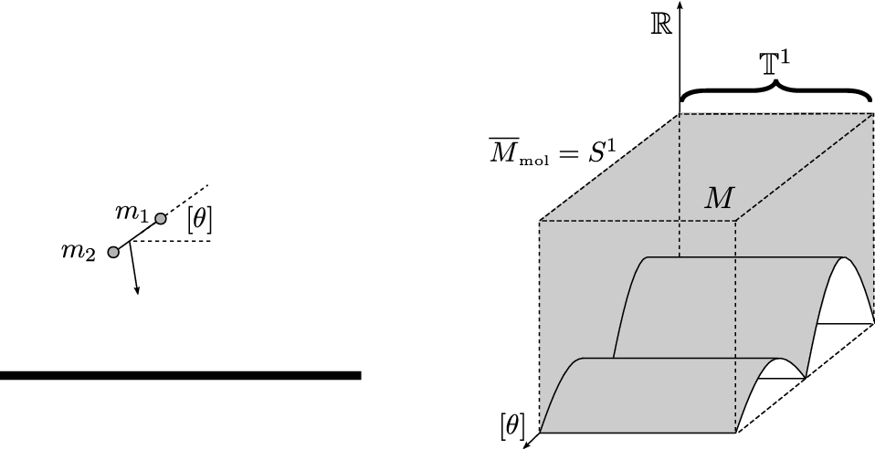
By restricting attention to a cross section ( constant) this -dimensional system can be reduced to a -dimensional system that is very much like the one of Figure 11, with taking the role of the length coordinate on in the first example. If we assume that is random, uniformly distributed, then we have a system that is of essentially of the same kind as that of the previous example.

Letting the normalized speed of the center of mass of the dumbbell molecule be the variable of interest (assuming, for simplicity, that the constant horizontal momentum is zero), then is regarded as a Markov operator with state space , where is the maximal speed that can be attained for a given, fixed, energy value. Writing for , the stationary distribution given by Proposition 8 has the form
It is easily shown that, for any initial probability distribution for , the corresponding Markov chain is (Lebesgue measure)-irreducible and aperiodic, and is the unique stationary probability measure.
Notice that does not depend on the length separating the two masses since changing only produces a homothety change of the rescaled region of Figure 13 (i.e., after the change of variables from to ). So only depends on the mass-ratio. Let . It is convenient to set . With this choice, the billiard cell contour in the coordinate plane is bounded below by the graph of the function
for
Based on the results and arguments from [6] and [8] one should expect to be an integral operator (Hilbert-Schmidt, or at least quasi-compact). We do not attempt to show this here, but only offer the numerical observation about the dependence of the spectral gap of on the mass-ratio parameter shown in Figure 14. The graph exhibits a great deal of structure which, at this moment, we do not know how to interpret.

4.2 Adding potentials
For an example with a non-constant potential function, consider the system on the left-hand side of Figure 15. This is similar to the two-masses system of Section 3 except that we add a linear spring potential acting on mass . Thus we consider a spring-mass with (essentially point) mass , which comprises the wall subsystem, and a point mass corresponding to the molecule subsystem. Suppose for simplicity that the free mass can only move vertically, so the whole set-up should be regarded as one-dimensional. It is assumed that there are no potentials involved other than the elastic potential of the spring. (In particular, no gravity.) Then is an interval, is a single point, the torus component has dimension , and is the subset of indicated on the right-hand side of the figure.
The region of interaction is the interval , where is a positive number. Let , indicate the positions of the masses and in physical space (on the left-hand side of the figure). Using the scaled coordinates
for the respective positions of and , the energy function for the system with linear spring potential is given by
The motion in between two collisions (of the two masses or of with the bottom wall or the semi-permeable wall at ) is given by the functions of :
| (4.2) |

The state variable of the Markov chain in this case is taken to be the speed of . It is assumed that the statistical state of is a Gibbs distribution with parameter . For concreteness, we describe chain transitions in algorithmic fashion:
- 1.
Choose independent, uniform random numbers , in , and a sign with equal probabilities;
- 2.
Let ; thus has probability density ;
- 3.
Let and thus has probability density proportional to over the interval where and is the spring potential in the scaled coordinate;
- 4.
Set to be the state of the mass when enters the region of interaction, and the state of . Let the system evolve, deterministically with this initial condition until is back at position . Along the way, assume that collisions with the boundary of the two dimensional region on the right side of Figure 15 are specular and in between collisions the trajectory satisfies equations 4.2. When reemerges at set equal to its new speed.
By Theorems 1 and 4, this Markov process has stationary probability given by the Maxwell-Boltzmann distribution (after reverting to the variables prior to scaling, with speed )
| (4.3) |

In comparing theses distributions with the corresponding textbook expressions, the reader should keep in mind the distinction between the Maxwell-Boltzmann distribution in the interior of billiard table (the gas container) and the similar distribution on the boundary surface (wall). The latter has density proportional to
in dimension , where is the unit normal to the wall surface.
5 Invariant volume forms
5.1 Definitions
Recall the function introduced in Subsection 1.2. The set is the level set . It will be convenient in this section to disregard the part of given by and consider as a submanifold of the boundary of . Observe that lies in the interior of the product region, where the molecule and wall subsystems are non-interacting. Thus it makes sense to define over a neighborhood of in the unit vector field along the -factor of . We choose the direction of so that it points towards the region of interaction. The restriction of to is then a unit vector field perpendicular to , pointing into . Let and , the pull-back of to under the inclusion map . Also define the subset of consisting of such that , , and . These are all bundles over . We often denote fibers of a bundle using subscripts, as in . When this is inconvenient, we use function form, so that , for example, is the fiber of above . Projection maps for these bundles will be denoted by the same symbol . Projection maps for other fibrations will typically be denoted by .
Clearly, the reflection map maps to and to itself. More generally, we can define as the restriction (pull-back) of to , and as we did in the case of . The notation may also be used when convenient. On regular points of the boundary, the reflection map is defined on . If we wish to emphasize that something is taking place over regular points of the boundary (or regular points of the function ), we may indicate this by adding a subscript such as in .
Let be a Riemannian metric on and the potential function. Unless explicitly stated otherwise, functions and tensor fields are assumed to be smooth on interior and regular boundary points. The Riemannian metric defines the kinetic energy function given by
The (total) energy function of the Newtonian system on with potential is such that
We write . Clearly, the base point projection maps into The intersection of with is denoted . Similar notations are used for the various related sets defined earlier. Whenever convenient, we specify points in simply by instead of . For example, we typically write , , , etc., for .
Let be the Levi-Civita covariant derivative operator. If is a vector field along a differentiable curve such that , the covariant derivative of along at will be written or, when appropriate, . The horizontal bundle over is the subbundle of defined as the kernel of the connection map , which is derived from as follows. Let , where is a differentiable curve in such that ; then
Write and . Let be a smooth section of over a neighborhood of such that and . Then .
Let denote the vertical bundle, which is the vector bundle over whose fiber above a is the tangent space to at . Thus is the kernel of , the projection is a linear isomorphism, and the direct sum decomposition holds. If is a smooth vector field on , then the horizontal lift of is the smooth section of given by
For each with , define the linear isomorphism , called the vertical lift map, by
The alternative notation or will also be used later instead of . If is a smooth vector field on , then the vertical lift of is the smooth section of given by
5.2 Contact, symplectic, and volume forms
The manifold is equipped with the canonical contact form defined by , for . It is well-known that is non-degenerate, hence a symplectic form on . In terms of the Riemannian metric,
| (5.1) |
from which it easily follows that is indeed non-degenerate and that and are Lagrangian subbundles.
The Hamiltonian vector field (associated to the energy function ) is the vector field on such that
| (5.2) |
One easily shows that and are invariant under . Thus and , where indicates the Lie derivative along . The contact form , however, is not in general invariant but satisfies , where is the Lagrangian function . The Hamiltonian vector field can be written as
| (5.3) |
where the geodesic spray is the vector field on defined, at each , as the horizontal lift of to . In particular, and . Observe that is a critical point of exactly when , which can only happen when and is critical for .
The Hamiltonian flow is the (local) flow of , which we denote by . The flow lines project under to curves on that satisfy Newton’s equation, and any solution of Newton’s equation lifts to a flow line in . It will be convenient to let represent a trajectory of the system through its entire history, which may include collisions and reflections with the boundary of . The Hamiltonian vector field is essentially complete, in the sense defined earlier in Section 1.2 (part (iv) of list of assumptions).
Proposition 9.
Let be a regular point for and let be either an interior point of or in the regular boundary . Then consists of such that
| (5.4) |
The projection is surjective. In fact, for each ,
satisfies . The space consists of all such that 5.4 holds and is tangent to .
Proof.
Proposition 10.
Let be the subset of of such that is a regular boundary point of and the inclusion map. Then is a symplectic form on . Furthermore, the reflection map leaves and invariant.
Proof.
Here and in what follows, we assume that all points under consideration are regular for and, if on the boundary, that they are regular boundary points. If , then is necessarily regular for . With this in mind, we omit references to ‘regular’ in the notation from now on.
The main issue is to check that is non-degenerate. Let and assume that for all , where is not tangent to the boundary of . First choose such that is orthogonal to . Then , so is orthogonal to all such that . That is, is a scalar multiple of . By Proposition 9 this vector is tangent to the boundary, thus zero by assumption, and must be a vertical vector. Let now be an arbitrary tangent vector to at . Then as and is tangent to we conclude that is a scalar multiple of the normal vector at , that is, for some . From Proposition 9 it follows that , which implies that . Therefore, ∎
It is useful to introduce the Sasaki metric on , which is the Riemannian metric defined by
for all and . In terms of this metric the vertical and horizontal subbundles are mutually orthogonal and , are isometric to under and , respectively.
Define the vector field
the gradient and norm being associated to the Sasaki metric. Observe that , so that where denotes the local flow of . It is not difficulty to obtain the expressions
where is the canonical vertical vector field, defined by for each .
Let , where . Then is a volume form (i.e., a non-vanishing form of top degree) on . It is also invariant under the Hamiltonian flow since .
Proposition 11.
Let be the Hamiltonian vector field for the energy function , and the vector field introduced in the previous paragraph. Define . Then
- 1.
;
- 2.
;
- 3.
It follows that the restriction of to each level set is non-vanishing (a volume form) and invariant under the Hamiltonian flow, and that the restriction of to the same level sets equals .
Proof.
For part 1, write and take the interior multiplication on both side with to conclude that . As does not vanish, we have . For part 2, observe that
But by the definition of and . Also . For part 3, obtain from that and take the interior multiplication on both sides of this equation with . ∎
5.3 Billiard maps
We fix an energy value and assume that has finite volume relative to . Here we will let denote more generally than before (the regular part of) a submanifold of the boundary of . For any given , define
which is if the flow line never returns to . By Poincaré’s recurrence applied to the Hamiltonian flow, is finite with probability with respect to the flow-invariant probability measure derived from . Now define the return map by being the reflection map. Then is almost everywhere defined, and by one of our standing assumptions it is almost surely smooth. (Section 1.2, assumption (v); see [3] for how this point concerning smoothness is argued in the simpler case of plane billiards.) We denote by the pull-back of to under the inclusion map. By Proposition 11 this form agrees with the pull-back of .
Proposition 12.
The return map preserves almost everywhere.
Proof.
This involves a standard argument, which we briefly recall. Let admit a neighborhood where is smooth. Let be the orbit segment connecting to , and a closed curve contained in . Let be a smooth embedded disc contained in that is bounded by , and denote by the image of under . Then sweeps out a surface under the Hamiltonian flow such that the boundary of is the union of and , where the negative sign indicates orientation. Notice that the restriction of to is as is constant on this surface and the interior multiplication of by the Hamiltonian vector field is . So
As and can be made arbitrarily small, we conclude that . Since also preserves according to Proposition 10, the same holds for . Therefore, leaves invariant as claimed. ∎
5.4 Product systems
We next specialize some of the above facts to product systems. The notation here is independent of that of the rest of the paper. Let . Let and be the tangent bundle maps and let be the projection . The induced projection will also be written , so it makes sense to write . If there is some possibility of confusion we may write, for example, instead of for a given in . Either way, the product Riemannian metric reads
Vertical and horizontal lifts, and the corresponding subbundles of decompose as expected in terms of the respective notions on . In particular, the Sasaki metric is similarly decomposed as . The canonical contact form on becomes , where is the contact form on , and the invariant volume form . Whenever convenient, we omit explicit reference to the projection maps and write, for example, or .
Assuming that the potential function on has the form , where is a smooth function on , the energy function becomes and the Hamiltonian vector field on is written as , where is characterized by being -related to the Hamiltonian vector field on associated to and -related to for . The (Sasaki) gradient of will be written, with slight abuse of notation, as and the vector field becomes
Proposition 13.
Let be the invariant volume form on the energy level and similarly define on level sets . Then the level sets can be measurably partitioned as a disjoint union of product manifolds
where the elements of the partition are the level sets of , and the invariant volume has the decomposition
adapted to this partition.
Proof.
The main point is to verify the stated form of . Define by . Now, can be written as
Since on , is an odd-degree form, and ,
as claimed. ∎
The Gibbs canonical distribution on with temperature parameter is the probability measure on defined by the form
where is a normalization constant. The following trivial but key observation must be noted.
Corollary 2.
If the states of the two subsystems are distributed according to the Gibbs canonical distribution with same parameter , then the state of the product system is also distributed according to the Gibbs canonical distribution with parameter .
Proof.
Let and define . Note that . Due to Proposition 13,
The measure obtained from is already normalized, so is the correct denominator. ∎
Theorem 1 can now be seen to follow from Corollary 2 and Proposition 1. If the state of the wall system has the Gibbs distribution with parameter and the state of the molecule system is given, prior to entering the interaction zone, the Gibbs distribution with the same parameter, then the state of the joint (product) system has a probability distribution which is invariant under the deterministic return map to the non-interaction zone. Thus the molecule factor of the state distribution of the total system upon return to the non-interaction zone remains the same.
5.5 Frame description of the volume forms
Let be the dimension of and an open subset on which is defined a smooth orthonormal frame of vector fields . Let be the subset of elements in with base point in . Define
Thus is an open submanifold of . Let denote the submanifold mapping to under . Let represent the standard basis of and the ordinary inner product. Observe that
is tangent to at a unit vector , and is a basis of for all not perpendicular to . For these , let be the dual basis associated to . In terms of this dual basis, the (standard) Riemannian volume form on is
| (5.5) |
This is obtained from , where the constitute the dual standard basis, by evaluating this form on the vectors . The Riemannian volume form on (up to sign) is
where the form the dual frame on . By identifying with and with , we may think of and as tangent to , and as a frame of -forms on .
We now introduce a diffeomorphism by
| (5.6) |
where . The inverse map is , where and .
Proposition 14.
For any given , define vectors and in by
If is a basis of and for some , then is a basis for , providing decompositions
where and are spanned by vectors of the form and , respectively. Define the forms . Letting , then
The vector field transforms under according to
Proof.
We only obtain and to illustrate the method of calculation. First, equals
where . Before calculating , first note that
where is a differentiable curve such that and , and indicates the parallel translation of along . Keeping in mind that and that , we obtain
The claimed identities are easily obtained from these. ∎
We have so far made no special assumptions about the local orthonormal frame . Since we may want to consider the invariant volume form near boundary points of , it makes sense to introduce the following concept: The orthonormal frame is said to be adapted to a codimension- foliation of if spans the tangent space to each leaf of at any given point . Recall that the set of elements in (respectively, in ) with base point in is denoted by (respectively, ). The set is easily seen to be a frame on . It was noted before that is a local, not necessarily orthonormal, frame on , and it can be shown exactly as in Proposition 9 that for a tangent vector to to actually be tangent to it is necessary and sufficient that its projection be tangent to . In particular, if is an adapted frame, the distribution in spanned by is involutive.
Proposition 15.
Define on the functions
where is an orthonormal frame on . The Hamiltonian vector field has the form
| (5.7) |
The contact form restricted to can be written as
| (5.8) |
where is the dual basis of . The volume form on each over the set can be written as
| (5.9) |
Now suppose that is adapted to a local codimension- foliation and let
| (5.10) |
be the restriction of to the leaves . Then is a symplectic form on each , and it can be written as
| (5.11) |
It follows that
| (5.12) |
The volume form transforms under the diffeomorphism defined by 5.6 according to
The symplectic form on a hypersurface in is expressed under according to
Proof.
All of this follows straightforwardly from the definitions and basic facts. We only make a few comments. Identity 5.9 results by noting that is a -form on , thus it can be written as , where the function is found by applying the interior multiplication with and using that is the coefficient of for the basis element . Item 2 of Proposition 11 is also needed. Identity 5.11 can be derived with little effort by using the identity 5.1, which expresses the symplectic form in terms of the Sasaki metric. Identity 5.12 is a consequence of 5.11 and the identity , where is the identity matrix, are column vectors, and is the row vector associated to after transpose. It should be kept in mind that the span an -dimensional subspace at each point, so they are linearly dependent. In fact, they satisfy the equation . ∎
Theorem 4 is a corollary of the proposition.
References
- [1] L. Breiman, Probability, Classics in Applied Mathematics, 7, SIAM, 1992.
- [2] C. Cercignani and D.H. Sattinger, Scaling Limits and Models in Physical Processes, DMV Seminar Band 28, Birkhäuser, 1998.
- [3] N. Chernov and R. Markarian, Chaotic Billiards, Mathematical Surveys and Monographs, 127, AMS, Providence, RI, 2006.
- [4] N. Chernov, D. Dolgopyat, Hyperbolic billiards and statistical physics, Proc. ICM (Madrid, Spain, 2006), Vol. II, Euro. Math. Soc., Zurich, 2006, 1679-1704.
- [5] F. Comets, S. Popov, G.M. Schutz, M. Vachkovskaia, Billiards in a general domain with random reflections. Arch. Ration. Mech. Anal. 191 (2008), 497-537.
- [6] R. Feres, Random walks derived from billiards, Dynamics, Ergodic Theory, and Geometry, Ed. B. Hasselblatt. Mathematical Sciences Research Institute Publications 54 (2007), 179–222.
- [7] R. Feres, G. Yablonsky, Knudsen’s cosine law and random billiards, Chemical Engineering Science, 59 (2004), 1541-1556.
- [8] R. Feres, H. Zhang, Spectral gap for a class of random billiards, to appear in Comm. of Math. Phys. (http://www.math.wustl.edu/feres/publications.html)
- [9] R. Feres, H. Zhang, The spectrum of the billiard Laplacian of a family of random billiards, Journal of Statistical Physics, V. 141, N. 6 (2010) 1030-1054.
- [10] J. Lee, Introduction to Smooth Manifolds, Springer 2003.
- [11] S. Meyn, R.L. Tweedie, Markov Chains and Stochastic Stability, second edition, Cambridge University Press, 2009.
- [12] W. A. Poor, Differential Geometry Structures, Dover, 2007.
- [13] G.O. Roberts, J.S. Rosenthal, Geometric Ergodicity and Hybrid Markov Chains, Elec. Comm. Prob. 2, 13-25, 1997.
- [14] R.J. Zimmer, Ergodic Theory and Semisimple Groups, Birkhäuser, 1983.