The Supermarket Game

The supermarket game is a simple model for analyzing distributed load balancing in transportation and communication networks. Load balancing ensures efficient resource utilization and improves the quality of service, by evenly distributing the workload across multiple servers. Traditionally, load balancing is fulfilled by a central dispatcher that assigns the newly arriving work to the server with the least workload. As modern or future networks become larger and increasingly distributed, such central dispatcher may not exist, and thus the load balancing has to be carried out by customers themselves. Hence, the supermarket game is relevant in scenarios where (1) customers choose which server to join without directions from a central dispatcher or tracker; (2) global workload or queue length information is not available and customers randomly choose a finite number of servers to probe; (3) there is cost associated with probing a server and waiting in a queue.

Examples of such scenarios are the following:

• •

  Network routing: customers represent traffic flows and servers represent possible routes from a given source to a destination. A traffic flow can find the route with low delay by probing different routes.

• •

  Dynamic wireless spectrum access: customers represent wireless devices and servers represent all the shared spectrum. The wireless devices can find the spectrum band with low interference and congestion by probing multiple spectrum bands.

• •

  Cloud computing service: customers can decide how many servers to probe in seeking the server with low delay.

In this paper, we address the following natural questions for these systems: How many servers will a self-interested customer sample? Is sampling or probing more servers by some customers beneficial or detrimental to the others?

The supermarket game with finite number of servers is difficult to analyze due to the correlation among queues at different servers. Therefore, we study the supermarket game in a mean field model that corresponds to the limit as the number of servers converges to infinity. By assuming: (1) unit exponential service rate at servers; (2) Poisson arrival of customers; (3) homogeneous waiting cost and sampling cost, it is shown that:

• •

  There exists a mixed strategy Nash equilibrium for all arrival rates per server less than one.

• •

  The action of sampling more servers by some customers has a positive externality on the other customers, which further implies that customers sample no more queues for any Nash equilibrium than for the socially optimal strategy.

• •

  Nash equilibrium is unique for arrival rates per server less than or equal to $1/\sqrt{2}$.

• •

  Nash equilibrium is unique if and only if a local monotonicity condition is satisfied. This condition is used to explore the uniqueness numerically for arrival rates per server larger than $1/\sqrt{2}$.

• •

  Multiple Nash equilibria exist for a particular example with arrival rates per server equal to $0.999$.

• •

  Nash equilibrium is unique for arrival rates per server equal to $0.999$ if customers can only sample either one queue or two queues.

Then, we consider the heterogenous waiting cost case and prove the existence of pure strategy Nash equilibrium in that case.

We also show that the mean field model arises naturally as the limit of supermarket game with finite number of servers:

• •

  A propagation of chaos result and a coupling result similar to the ones in [7] and [20] hold, and thus the joint equilibrium distribution of any fixed number of queues converges to a product distribution determined by the mean field model as the number of queues converge to infinity.

• •

  A Nash equilibrium of the supermarket game in the mean field model is an $\epsilon$-Nash equilibrium of the supermarket game for finite number of servers with the number of servers large enough.

Furthermore, in the supermarket game with finite number of servers, we find that sampling more queues by some customers has a nonnegative externality on customers who only sample one queue, but it can have a negative externality for customers sampling more than one queue, which is in sharp contrast to the conclusion in the mean field model.

The supermarket game is formulated based on the classical supermarket model with $N$ parallel queues in which customers sample a fixed number $L$ of queues uniformly at random and join the shortest sampled queue. The supermarket model has been extensively studied in the literature using the mean field approach. Vvedenskaya et. al. [21] shows that in the mean field model, the equilibrium queue sizes decay doubly exponentially for $L\geq 2$. Turner [20] proves an interesting coupling result for fixed $N$, which implies that the load in the network is handled better and more evenly as $L$ increases. Graham [7] proves a chaoticity result on the path space using the idea of propagation of chaos [17], and Mitzenmacher [16] studies the model using Kurtz’s theorem. Furthermore, Luczak and McDiarmid [14] prove that for $L\geq 2$, the maximum queue length scales as $\ln\ln n/\ln L+O(1)$. The recent paper by Bramson et. al. [3] analyzes the supermarket model with general service time distributions. They show that in the case of FCFS discipline and power-law service time, the equilibrium queue sizes will decay doubly exponentially, exponentially, or just polynomially, depending on the power-law exponent and the number of choices $L$. Ganesh et. al. [6] studies a variant of the supermarket model, where the customers initially join an arbitrary server, but may switch to other servers later independently at random. They find that in the mean field model, the average waiting time under the load-oblivious switching strategy is not considerably larger than that under a smarter load-aware switching strategy.

In addition to the supermarket model, the mean field approach has also been used to analyze scheduling in queueing networks, such as the CSMA algorithm in a wireless local area network [2] and downlink transmission scheduling [1]. Also, a recent work [18, 19] investigates the performance tradeoff between centralized and distributed scheduling in a multi-server system for the mean field model. However, none of above work considers a game-theoretic framework.

The supermarket game proposed in this paper falls into a large research area involving equilibrium behavior of customers and servers, known as queueing games. A comprehensive survey can be found in [9]. A particularly relevant paper by Hassin and Haviv [8] studies a two line queueing system, where upon arrival each customer decides whether to purchase the information about which line is shorter, or randomly select one of the lines. It shows how to find a Nash equilibrium and examines the externality imposed by an informed customer on the others. A model in which customers can balk, either before or after sampling the backlog at a single server queue, is considered in [10]. the paper finds benefits to the service operator of offering the possibility to balk after the backlog is sampled.

Finally, the supermarket game is also related to and partially motivated by the theory of mean field games in the context of dynamical games [11, 13]. The mean field game approach studies a weakly coupled, $N$ player game by letting $N\to\infty$. However, we caution that in the supermarket game, we consider an infinite sequence of customers instead of finitely many customers, which is different from an $N$ player game.

Section 2 introduces the precise definition of the supermarket game to be studied and the key notations. The mean field model for the supermarket game is studied in Section 3, and justified in Section 4. Section 5 examines the externality of sampling more queues in the finite $N$ model. Section 6 ends the paper with concluding remarks. Miscellaneous details and proofs are in the Appendix.

Consider a supermarket game with $N$ FCFS queues with exponential service rate one, and global Poisson arrival rate $N\lambda$. Assume $\lambda<1$ and let $\mathcal{L}=\{1,\ldots,L_{\rm max}\}$. Upon arrival, each customer can choose a number $L\in\mathcal{L}$ of queues to be sampled uniformly at random, and the customer joins the sampled queue with the least number of customers, ties being resolved uniformly at random. Customers are assumed to have cost $c$ per unit waiting time and $c_{s}$ for sampling one queue. These cost parameters are the same for all the customers; heterogeneous waiting costs are only considered in Section 3.6.

For a fixed customer $i$, if she chooses $L_{i}$ queues to sample, and all the other customers choose $L_{-i}$, then by PASTA (Poisson arrival sees time average), the expected total cost of customer $i$ is given by

where $\mathbb{E}[W(L_{i},L_{-i})]$ is the expected waiting time (service time included) under the stationary distribution. The goal of customer $i$ is to minimize her own expected total cost by choosing the optimal $L_{i}$.

Since the supermarket game is symmetric in the customers, we limit ourselves to symmetric strategies. We call $L^{\star}\in\mathcal{L}$ a pure strategy Nash equilibrium, if

Since a pure strategy Nash equilibrium does not always exist, we are also interested in mixed strategy Nash equilibria.

Let $\mathcal{P}(\mathcal{L})$ denote the set of all probability distributions over $\mathcal{L}$. The mixed strategy $\mu_{i}$ for customer $i$ is simply a probability distribution in $\mathcal{P}(\mathcal{L})$, i.e., $\mu_{i}(L_{i})$ is the probability that customer $i$ samples $L_{i}$ queues. If all the other customers use the mixed strategy $\mu_{-i}$, then the expected total cost of customer $i$ using $\mu_{i}$ is given by

where $C(L_{i},\mu_{-i})$ is the expected total cost of customer $i$ choosing $L_{i}$ given all the others choose the mixed strategy $\mu_{-i}$.

Define the best response correspondence for customer $i$ as $\text{BR}(\mu_{-i}):=\arg\min_{\mu_{i}}C(\mu_{i},\mu_{-i})$. The correspondence BR is a set-valued function from $\mathcal{P}(\mathcal{L})$ to subsets of $\mathcal{P}(\mathcal{L})$. We call $\mu^{\star}\in\mathcal{P}(\mathcal{L})$ a mixed strategy Nash equilibrium if

In this paper, we are interested in characterizing the Nash equilibria of the supermarket game.

Let $\mathscr{X}$ denote a separable and complete metric space, $\mathcal{M}(\mathscr{X})$ and $\mathcal{P}(\mathscr{X})$ be the space of measures and space of probability measures on $\mathscr{X}$, respectively. In this paper, $\mathscr{X}$ will be $\mathcal{L}$, $\mathbb{N}$, $\mathbb{D}(\mathbb{R}_{+},\mathbb{N})$, or the space of probability measures on these spaces, where $\mathbb{N}$ is the set of natural numbers and $\mathbb{D}$ denotes the Skorokhod space. Let $\mathscr{L}(X)$ denote the law of a random variable $X$ on $\mathscr{X}$ and $\delta_{x}$ denote a point probability measure at $x\in\mathscr{X}$. Weak convergence of probability measures is denoted by $\Longrightarrow$.

Define on $\mathcal{M}(\mathscr{X})$ natural duality brackets with $L^{\infty}(\mathscr{X})$ as: for $\phi\in L^{\infty}(\mathscr{X})$ and $\mu\in\mathcal{M}(\mathscr{X})$, $\langle\phi,\mu\rangle=\int\phi d\mu$. Without ambiguity, brackets are also used to denote the quadratic covariation of continuous time martingales: let $M_{1},M_{2}$ be two continuous time martingales, then $\langle M_{1},M_{2}\rangle$ is the standard quadratic covariation process. Define the total variation norm on $\mathcal{M}(\mathscr{X})$ as $\|\mu\|_{\rm TV}=\sup\{\langle f,\mu\rangle:\|f\|_{\infty}\leq 1\}$. Let $\|\mu_{1}-\mu_{2}\|_{\rm TV}$ be the corresponding total variation distance.

For $\mu_{1},\mu_{2}\in\mathcal{P}(\mathcal{L})$, use $\mu_{1}\leq_{\rm st}\mu_{2}$ to denote that $\mu_{1}$ is first-order stochastically dominated by $\mu_{2}$, i.e., $\sum_{j=l}^{L_{\max}}\mu_{1}(j)\leq\sum_{j=l}^{L_{\max}}\mu_{2}(j),\forall l\in\mathcal{L}$. For $x\in\mathbb{R}$, let $\lfloor x\rfloor$ denote the maximum integer no larger than $x$.

In this subsection, we derive an expression for the expected total cost incurred by a customer in a mean field model, by assuming that queue lengths (including customers in service) are independent and identically distributed.

Suppose all the customers except customer $i$ use the mixed strategy $\mu_{-i}$, and let $r_{t}(k)$ denote the fraction of queues with at least $k$ customers at time $t$ in the mean field model. Then, the mean field equation is given by

which is rigorously derived in Section 4. For now, let us provide some intuition for each of the drift terms in (3.1):

The term $\lambda\mu_{-i}(l)(r_{t}^{l}(k-1)-r_{t}^{l}(k))$ corresponds to the arrivals of customers sampling $l$ queues. Because queue lengths are i.i.d, $r_{t}^{l}(k-1)$ is the probability that the minimum queue length of $l$ uniformly sampled queues is greater than or equal to $k-1$. Thus, $(r_{t}^{l}(k-1)-r_{t}^{l}(k))$ is the probability that the minimum queue length of $l$ uniformly sampled queues is $k-1$, which is the same as the probability that a customer who samples $l$ queues joins a queue with $k-1$ customers. Note that $r_{t}(k)$ is increased if a customer joins a queue with $k-1$ customers. Therefore, $\sum_{l=1}^{L_{\rm max}}\lambda\mu_{-i}(l)\left(r_{t}^{l}(k-1)-r_{t}^{l}(k)\right)$ is the aggregate drift for $r_{t}(k)$ corresponding to arrivals.

The term $(r_{t}(k)-r_{t}(k+1))$ corresponds to departures of customers at queues with exactly $k$ customers.

Since we are interested in the stationary regime, set $\frac{dr_{t}(k)}{dt}=0$ to yield equations for the equilibrium distribution denoted by $r_{\mu_{-i}}(k),k\geq 0$. For $k\geq 1$,

where the random variable $\mathbf{L}$ is distributed as ${\mu_{-i}}$. By summing the above equation for $k_{0}\leq k<+\infty$ using telescoping sums and changing $k_{0}$ to $k$, it follows that

where $u_{\mu_{-i}}(x):=\mathbb{E}_{\mu_{-i}}\left[x^{\mathbf{L}}\right]=\sum_{l=1}^{L_{\max}}x^{l}{\mu_{-i}}(l)$.

Because queues are independent in the mean field model,

where $N(L_{i})$ is the length of the shortest queue among the $L_{i}$ sampled queues. Therefore,

Since $g(L)=x^{L}$ is convex in $L\in\mathbb{R}$ for $x\geq 0$ and strictly convex for $0<x<1$, it follows that $\mathbb{E}[W(L,\mu_{-i})]$ and $C(L,\mu_{-i})$ are strictly convex in $L\in\mathbb{R}$.

Next, we prove several key lemmas which are useful in the sequel.

Let $\mu_{i}\in\text{BR}(\mu_{-i})$. Suppose there exists $L_{1}<L_{2}<L_{3}\in\mathcal{L}$ such that $\mu_{i}(L_{1})>0$ and $\mu_{i}(L_{3})>0$. Then, by the definition of BR,

which contradicts the fact that $C(L,\mu_{-i})$ is strictly convex in $L$ and thus the conclusion follows. ∎

The next lemma translates the stochastic dominance relations between strategies into the stochastic dominance relations between mean field equilibrium distributions.

Since $\mu_{1}\leq_{\rm st}\mu_{2}$, it follows that for all $x\in[0,1]$, $u_{\mu_{1}}(x)\geq u_{\mu_{2}}(x)$. We prove the lemma by induction. If $k=0$, then $r_{\mu_{1}}(0)=r_{\mu_{2}}(0)=1$ and $r_{\mu_{1}}(0)\geq r_{\mu_{2}}(0)$ trivially holds. If $r_{\mu_{1}}(k-1)\geq r_{\mu_{2}}(k-1)$, then

Therefore, for all $k\in\mathbb{N}$, $r_{\mu_{1}}(k)\geq r_{\mu_{2}}(k)$. Moreover, if $\mu_{1}<_{\rm st}\mu_{2}$, it follows that for all $x\in(0,1)$, $u_{\mu_{1}}(x)>u_{\mu_{2}}(x)$. Thus, for all $k\geq 2$, $r_{\mu_{1}}(k)>r_{\mu_{2}}(k)$.

Let $\mu_{1}=\delta_{1}$ be a point measure at singleton $1$. Then, $r_{\mu_{1}}(k)=\lambda^{k}$. Because for any $\mu\in\mathcal{P}(\mathcal{L})$, $\delta_{1}\leq_{\rm st}\mu$, then $r_{\mu}(k)\leq\lambda^{k}$ and $C(L,\mu)\leq c/(1-\lambda)+c_{s}L_{\max}$. ∎

The next lemma states that $C(\mu_{i},\mu_{-i})$ is a continuous function.

See the proof in Appendix A.1. ∎

In this subsection, we show the existence of a mixed strategy Nash equilibrium. It is easy to see that if there exists $\mu^{\star}$ with $\mu^{\star}\in\text{BR}(\mu^{\star})$, i.e., $\mu^{\star}$ is a fixed point of the best response correspondence, then $\mu^{\star}$ is a mixed strategy Nash equilibrium. Thus, it suffices to show the existence of such a fixed point. The Kakutani fixed point theorem is used to prove it.

In our setting, $\mathcal{S}=\mathcal{P}(\mathcal{L})$ and $g=\text{BR}$. It is known that $\mathcal{P}(\mathcal{L})$, as a space of probability distribution on finite set, is a nonempty, compact and convex subset of some Euclidean space. Also, since $C(\mu_{i},\mu_{-i})$ is continuous, by Weierstrass Theorem, $\text{BR}(\mu_{-i})$ is a nonempty set. In addition, $C(\mu_{i},\mu_{-i})$ is linear in $\mu_{i}$, so $\text{BR}(\mu_{-i})$ is a convex set. The last and key step is to prove that BR has a closed graph, i.e., suppose $\mu_{-i}^{(n)}\to\mu_{-i}$, $\mu_{i}^{(n)}\in\text{BR}(\mu_{-i}^{(n)})$ and $\mu_{i}^{(n)}\to\mu_{i}$, we need to show that $\mu_{i}\in\text{BR}(\mu_{-i})$. It is proved in the following theorem using the continuity of $C(\mu_{i},\mu_{-i})$.

See the proof in Appendix A.2. ∎

The uniqueness of mixed strategy Nash equilibrium is proved next in case $\lambda^{2}\leq 1/2$. Some definitions and lemmas are introduced first.

For customer $i$, her marginal value of sampling at an integer $L_{i}$ with all the others adopting $\mu_{-i}$, is defined as

Intuitively, $V(L_{i},\mu_{-i})$ characterizes the reduction of expected waiting time when customer $i$ increases the number of sampled queues from $L_{i}$ to $L_{i}+1$. For ease of notation, define $V(0,\mu_{i})=\infty$ and $V(L_{\max},\mu_{i})=0$. Since $\mathbb{E}[W(L_{i},\mu_{-i})]$ is strictly convex in $L\in\mathbb{R}$, $V(L_{i},\mu_{-i})$ is strictly decreasing in $L_{i}$. The following lemma characterizes the best response using $V(L_{i},\mu_{-i})$.

See the proof in Appendix A.3. ∎

The next lemma proves a global monotonicity property of $V(L_{i},\mu_{-i})$ in case $\lambda^{2}\leq 1/2$, which is useful for showing the uniqueness of Nash equilibrium in that case.

See the proof in Appendix A.4. ∎

Lemma 5 implies that for $\lambda^{2}\leq 1/2$, a customer tends to sample fewer queues when all the other customers sample more queues. This is an instance of avoid the crowd behavior [9], leading to uniqueness of the Nash equilibrium.

A Nash equilibrium exists by Theorem 1. Let $L^{\star},\tilde{L}^{\star}\in[1,L_{\max}]$ denote two possible Nash equilibria; we show that $L^{\star}=\tilde{L}^{\star}$.

Without loss of generality, suppose $L^{\star}<\tilde{L}^{\star}$; by Lemma 5, $L^{\star}\geq\tilde{L}^{\star}$, which is a contradiction and concludes the proof. ∎

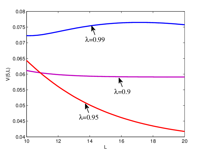
However, the marginal value of sampling $V(L_{i},L_{-i})$ is not always increasing in $L_{-i}\in[1,L_{\max}]$ ($L_{-i}$ refers to a probability distribution here) for all $\lambda<1$. By numerical results, we find that when $\lambda=0.99$ and $L_{i}=5$, $V(L_{i},L_{-i})$ is increasing with $L_{-i}$ for $11\leq L_{-i}\leq 16$, as shown in Fig. 1. This implies that sometimes a customer tends to sample more queues when all the others sample more queues. This follow the crowd behavior can lead to multiple Nash equilibria. Such a scenario is described in the next subsection.

In this subsection, we show how to find a Nash equilibrium and establish the uniqueness of Nash equilibrium if a local monotonicity condition is satisfied. Then, a specific example where multiple Nash equilibria exist is constructed.

The following lemma determines a Nash equilibrium using the marginal value of sampling.

See the proof in Appendix A.5. ∎

Next, we introduce a local monotonicity condition and show the uniqueness of Nash equilibrium for all values of $c$ and $c_{s}$ if and only if the local monotonicity condition is satisfied.

See the proof in Appendix A.6. ∎

The following numerical results, depicted in Fig. 2, show that when $\lambda=0.99$, $V(L,L+q)$ is indeed strictly decreasing with respect to $0\leq q\leq 1$ for $L=1,\ldots,9$. For $L\geq 10$,

which implies that $V(L,L+q)$ is strictly decreasing over $0\leq q\leq 1$, in view of the proof for Lemma 5. Therefore, for $\lambda=0.99$ and any integer $L_{\max}\geq 1$, there exists a unique Nash equilibrium for all values of $c$ and $c_{s}$.

However, when $\lambda=0.999$ and $L_{\max}=25$, $V(L,L+q)$ is strictly increasing in $q$ for $L=18,\ldots,24$. Therefore, multiple Nash equilibria exist if $c_{s}/c=0.0148$, as depicted in Fig. 3. We see that $L=19,\ldots,24$ are pure strategy Nash equilibria and mixed strategy Nash equilibria exist between each two consecutive pure strategy Nash equilibria.

In this subsection, we consider a simple special case where all the customers only have two choices, $1$ or $2$.

Fixing a customer $i$, if $L_{-i}=1+q$, i.e., all the other customers choose one queue to sample with probability $1-q$ and two queues with probability $q$, then the stationary distribution in the mean field model can be derived as

where $u_{q}(x)=x^{2}q+x(1-q)$. Note that this stationary distribution has also been derived in Section 4.4.1 of[15].

Then, the total expected cost of customer $i$ choosing $1+p$ is given by

The marginal value of sampling of customer $i$ at $1$ is given by

It follows that the best response under $L_{-i}=1+q$ is given by

By numerical results depicted in Fig. 4, we find that $V(1,1+q)$ is strictly decreasing in $q$ for a sequence of $\lambda$ up to $0.999$. This is strong numerical evidence that the local monotonicity condition is satisfied for all $\lambda<1$. Therefore, by Theorem 3 and Lemma 4, we conjecture that: (i) if $V(1,1)\leq c_{s}/c$, then $L^{\star}=1$ is the unique Nash equilibrium; (ii) if $V(1,2)\geq c_{s}/c$, then $L^{\star}=2$ is the unique Nash equilibrium; (iii) otherwise, there exists a $p^{\star}\in(0,1)$ such that $V(1,1+p^{\star})=c_{s}/c$, and thus $L^{\star}=1+p^{\star}$ is the unique mixed strategy Nash equilibrium.

The action of sampling more queues by some customers has an effect on the waiting time of others. This effect is called the externality associated with the action and the externality is positive if the action reduces the mean waiting time of the other customers. In this subsection, the externality in the mean field model is analyzed. It is not clear whether the externality is positive at first sight. On one hand, choosing a large number of queues to sample helps a customer find a less loaded queue and hence reduces future arrivals’ opportunity to find lightly loaded queues. On the other hand, it also leads to a well balanced system and reduces the average waiting time.

The following corollary of Lemma 2 implies that the action of sampling more queues by some customers has a positive externality on the other customers in the mean field model. To see it, suppose in system 1, all the customers adopt a strategy $\mu_{1}$; while in system 2, a fraction $0<p\leq 1$ of them samples more queues, i.e., adopts a new strategy $\mu_{3}$ with $\mu_{1}<_{\rm st}\mu_{3}$ and all the others still adopt the strategy $\mu_{1}$. For system $2$, it is equivalent to assume that all the customers adopt a strategy $\mu_{2}$ with $\mu_{2}=p\mu_{3}+(1-p)\mu_{1}$. It follows that $\mu_{1}<_{\rm st}\mu_{2}$. By Corollary 1, system 2 has smaller mean waiting time.

Because $\mu_{1}<_{\rm st}\mu_{2}$, by Lemma 2, $r_{\mu_{1}}(k)>r_{\mu_{2}}(k),\forall k\geq 2$. Hence, the conclusion follows by invoking the definition of $\mathbb{E}[W(L,\mu)]$. ∎

Next, we analyze the social optimum, i.e, the minimum of total cost of all the customers. Suppose all the customers use the mixed strategy $\mu$; the expected total cost per unit time $C_{\rm sum}(\mu)$ is given by

Therefore, a minimizer of the following minimization problem:

is a social optimum.

See the proof in Appendix A.7. ∎

The total cost can be decomposed into two terms as

Suppose the Nash equilibrium $\mu^{\star}>_{\rm st}\mu^{\star}_{\rm soc}$, then by the positive externality result, we have

Also, by definition of $\mu^{\star}$,

Therefore,

which is a contradiction to the definition of $\mu_{\rm soc}^{\star}$. ∎

In this subsection, the heterogeneous waiting cost is considered. In particular, assume that there is a nondegenerate continuous probability density function for waiting cost $c$, i.e., $\int_{0}^{c_{\max}}f(c)dc=1$.

Fix a customer $i$, let $L_{i}(\cdot)$ denote a function from $[0,c_{\max}]$ to $\mathcal{L}$. We call $L_{i}(\cdot)$ the strategy of customer $i$. In particular, if customer $i$ has a waiting cost $c$, then she chooses $L_{i}(c)$ queues to sample uniformly at random. Now suppose all the other customers use $L_{-i}(\cdot)$, the expected total cost for customer $i$ is given by

The goal of customer $i$ is to minimize the expected total cost by choosing the optimal $L_{i}(\cdot)$. Define the best response correspondence as $\text{BR}(L_{-i}(\cdot)):=\arg\min_{L_{i}(\cdot)}C(L_{i},L_{-i})$.

If $L_{i}(\cdot)\in\text{BR}(L_{-i}(\cdot))$, then $L_{i}(\cdot)$ must be a nondecreasing step function with respect to $c$ as depicted in Fig. 5, which is proved in the following lemma.

Suppose $0\leq c<\hat{c}\leq c_{\max}$, since $L_{i}(\cdot)\in\text{BR}(L_{-i}(\cdot))$, we have

Adding the above two inequalities up, we get

Therefore $\mathbb{E}[W(L_{i}(\hat{c}),L_{-i})]\leq\mathbb{E}[W(L_{i}(c),L_{-i})]$ and thus $L_{i}(\hat{c})\geq L_{i}(c)$. ∎

Define the strategy space $\mathcal{S}$ as the collection of all possible nondecreasing step functions from $[0,c_{\max}]$ to $\mathcal{L}$. By Lemma 8, it suffices to consider $\mathcal{S}$ for finding pure strategy Nash equilibrium. There is a bijective mapping between the strategy space $\mathcal{S}$ and probability space $\mathcal{P}(\mathcal{L})$. In particular, suppose $L(\cdot)\in\mathcal{S}$ is given, and let $0=c_{0}<c_{1}<\cdots<c_{L_{\max}}=c_{\max}$ denote the jumping points. Then, define $\mu(l)=\int_{c_{l-1}}^{c_{l}}f(c)dc$. On the other hand, suppose $\mu\in\mathcal{P}(\mathcal{L})$ is given, then the equation $\mu(l)=\int_{c_{l-1}}^{c_{l}}f(c)dc$ is solved to get the unique jumping points $0=c_{0}<c_{1}<\cdots<c_{L_{\max}}=c_{\max}$. Thus, $L(\cdot)$ can be constructed as $L(c)=l$ for $c_{l-1}\leq c<c_{l}$. Define a metric on the strategy space $\mathcal{S}$ as $d(L_{1}(\cdot),L_{2}(\cdot)):=\|\mu_{L_{1}}-\mu_{L_{2}}\|$. Also, Let $F$ denote the bijective mapping from $L(\cdot)$ to $\mu_{L}$ and $F^{-1}$ denote the inverse mapping. It is easy to see that $F$ and $F^{-1}$ are continuous.

References

- [1] Alanyali, M. and Dashouk, M. (2011). Occupancy distributions of homogeneous queueing systems under opportunistic scheduling. IEEE Transactions on Information Theory 57, 1 (Jan.), 256 –266.
- [2] Bordenava, C., McDonald, D., and Proutiere, A. (2010). A particle system in interaction with a rapidly varying environment: Mean field limits and applications. Journal on Networks and Heterogeneous Media 5, 31–62.
- [3] Bramson, M., Lu, Y., and Prabhakar, B. (2010). Randomized load balancing with general service time distributions. In Proceedings of the ACM SIGMETRICS 2010. New York, NY, USA, 275–286.
- [4] Deimling, K. (1977). Ordinary Differential Equations in Banach Spaces. Vol. 96. Springer.
- [5] Ethier, S. and Kurtz, T. (1986). Markov Processes: Characterization and Convergence. John wiley, New York.
- [6] Ganesh, A., Lilienthal, S., Manjunath, D., Proutiere, A., and Simatos, F. (2010). Load balancing via random local search in closed and open systems. SIGMETRICS Perform. Eval. Rev. 38, 287–298.
- [7] Graham, C. (2000). Chaoticity on path space for a queueing network with selection of the shortest queue among several. Appl. Prob. 37, 198–211.
- [8] Hassin, R. and Haviv, M. (1994). Equilibrium strategies and the value of informaiton in a two line queueing system with threshold jockeying. Commun. Statist. Stochastic Models 10(2), 415–435.
- [9] Hassin, R. and Haviv, M. (2003). To queue or not to queue: equilibrium behavior in queueing systems. International series in Operations Research and Management Science, Springer.
- [10] Hassin, R. and Roet-Green, R. Equilibrium in a two dimensional queueing game: When inspecting the queue is costly. preprint (Dec. 2012), available at http://www.math.tau.ac.il/ hassin/ricky.pdf.
- [11] Huang, M., Caines, P., and Malhame, R. (2007). Large-population cost-coupled LQG problems with nonuniform agents: Individual-mass behavior and decentralized -Nash equilibria. IEEE Transactions on Automatic Control 52, 9 (Sept.), 1560 –1571.
- [12] Kingman, J. (1966). Two similar queues in parallel. Annals of Mathematical Statistics 32, 1314–1323.
- [13] Lasry, J. M. and Lions, P. L. (2007). Mean field games. Japanese Journal of Mathematics, 229–260.
- [14] Luczak, M. and McDiarmid, C. (2006). On the maximum queue length in the supermarket model. Ann. Probab. 34, 493–527.
- [15] Mitzenmacher, M. (1996). The power of two choices in randomized load balancing. Ph.D. thesis, Univ. of California, Berkeley.
- [16] Mitzenmacher, M. (2001). The power of two choices in randomized load balancing. IEEE Trans. on Parallel and Distributed Systems 12:10, 1094–1104.
- [17] Sznitman, A. (1991). Topics in propagation of chaos. In Springer Verlag Lecture Notes in Mathematics 1464, P. Hennequin, Ed. Springer-Verlag, 165–251.
- [18] Tsitsiklis, J. N. and Xu, K. (2011). On the power of (even a little) centralization in distributed processing. SIGMETRICS Perform. Eval. Rev. 39, 121–132.
- [19] Tsitsiklis, J. N. and Xu, K. (2012). On the power of (even a little) resource pooling. Stochastic Systems 2, 1–66.
- [20] Turner, S. (1998). The effect of increasing routing choice on resource pooling. Prob. Eng. Inf. Sci. 12, 109–123.
- [21] Vvedenskaya, N. D., Dobrushin, R. L., and Karpelevich, F. I. (1996). Queueing system with selection of the shortest of two queues: An asymptotic approach. Prob. Inf. Trans 32, 15–27.