Models for Modules
The Story of O
Jan Troost
Laboratoire de Physique Théorique11 1 Unité Mixte du CNRS et de l’Ecole Normale Supérieure associée à l’Université Pierre et Marie Curie 6, UMR 8549.
Ecole Normale Supérieure
24 rue Lhomond, 75005 Paris, France
Abstract: We recall the structure of the indecomposable modules in the Bernstein-Gelfand-Gelfand category . We show that all these modules can arise as quantized phase spaces of physical models. In particular, we demonstrate in a path integral discretization how a redefined action of the algebra over the complex numbers can glue finite dimensional and infinite dimensional highest weight representations into indecomposable wholes. Furthermore, we discuss how projective cover representations arise in the tensor product of finite dimensional and Verma modules and give explicit tensor product decomposition rules. The tensor product spaces can be realized in terms of product path integrals. Finally, we discuss relations of our results to brane quantization and cohomological calculations in string theory.
1 Motivations
The study of quantum physics mostly takes place in the arena of unitary Hamiltonian time evolution in a Hilbert space of physical states with positive norm. In many contexts though it turns out to be useful to temporarily extend the arena of analysis to non-unitary systems. This is true for example for open systems or for the extension of unitary field theory Lagrangians to complexified coupling constants. It is also frequently useful to render the action of a symmetry manifestly covariant, and this can also lead to the introduction of null or negative norm states. The latter possibility arises in the study of physical systems with a gauge symmetry, which includes many of the basic theories of nature. Thus we may wish to temporarily study non-unitary state spaces for physical systems.
In this paper, we study state spaces for systems with symmetry, where denotes the three-dimensional Lie algebra over the complex numbers. The state spaces will not necessarily allow for an invariant positive norm. Our goal is to generalize the construction of a classical geometrical system whose path integral quantization gives rise to spin [1, 2, 3]. The geometrical picture of finite dimensional representations was inherited from the mathematical literature on the quantization of coadjoint orbits of Lie groups [4, 5, 6, 7]. It applies to representations that arise in the space of quadratically integrable functions on the group. We broaden the path integral treatment to include more general representations of . The generalization can be viewed as part of a program to render algebra geometric.
We will concentrate on modules with a finite number of highest weight states22 2 We take the mathematics convention here. In physics, we more often discuss representations with a finite number of lowest weight states.. More precisely, we will concentrate on the Bernstein-Gelfand-Gelfand category of modules. These are modules that are finitely generated, that can be decomposed into weight spaces, and that are locally finite with respect to the action of raising operators (see e.g. [8]). These modules are classified. There are examples amongst these modules that appear in various physical contexts. These include the analytic continuation of modules to modules (e.g. in analytically continuing spaces of states on euclidean to Lorentzian [9][10]), and open string representation spaces in the topological A-model on the complexified sphere [11].
We were motivated for this study by the fact that if one considers representations of the conformal group with lowest weight, and a set of supersymmetry generators acting on those representations, one will generate representations of the type that we analyze. Equivalently, they arise from the action of fermionic generators on representations of an isometry group. We provide an opportunity for understanding the appearance of projective modules and a non-diagonalizable action of Casimirs in these contexts, using elementary physical models. These algebraic phenomena are key in determining the space of physical states in Berkovits models of superstrings on backgrounds with Ramond-Ramond flux [12][13][14].
2 Representations
In this section we review the Bernstein-Gelfand-Gelfand (BGG) category of modules. We refer the reader to the book [8] for a detailed and pedagogical exposition.
2.1 The BGG category
The algebra is generated by the three generators that satisfy the commutation relations:
| (2.1) |
We will concentrate on the modules of this algebra that can be generated from a finite set of vectors. Moreover, the modules can be decomposed into modules of given weight with respect to a Cartan subalgebra, and each vector only generates a finite dimensional subspace when we act on it with raising operators only. The indecomposable modules inside this category of modules have been classified (see e.g. [8]). All other modules are direct sums of these. We review the indecomposable modules next.
2.2 The indecomposable modules
For any highest weight , we have a Verma module which is generated by the free action of the lowering operators. It contains weights . When is a positive integer, we have that the module has a finite dimensional simple module of dimension as a quotient. In that case, we have the short exact sequence .
The category also contains the modules dual to the Verma modules. The duality operation is such that it acts within the BGG category . The action of the generators on the vector space dual to the original one is given by: , and where the vector is in the original vector space and is a map in the dual. The modules have the property that one can go from any state to the highest weight state by ascent. This is dual to the property that in a Verma module , we can reach any state from the highest weight state by descent. When is a positive integer, we have the short exact sequence .
Finally, there are non-trivial projective modules for a positive integer. These modules are indecomposable, have a submodule and they fit into the short exact sequence . In fact, they also fit into the dual short exact sequence . They are the largest indecomposable modules that cover the Verma module (when is a positive integer).
For the reader not familiar with these representations or their description in terms of short exact sequences, it may prove useful to study the modules in detail, using the explicit formulas given in appendix A. For more on the construction of the BGG category, on simple, Verma and projective modules, we must refer to [8] and references therein.
3 Quantizations
In this section, we wish to realize the representations of section 2 in terms of phase spaces of models with a path integral formulation. For each of the representations, we will specify the phase space, and the expression of the generators of in the path integral formalism, such that the quantum phase space becomes the desired representation space. We hereby generalize the path integral quantization of spin [1][2][3].
3.1 The finite dimensional representations
We first review the finite dimensional representations of , and their realization in a physical system.
3.1.1 Orbit quantization
The finite dimensional representations are unitary representations of the real form of the algebra . They arise as Hilbert spaces from the geometric quantization of the orbits of the Lie algebra [4, 5, 6, 7]. A path integral quantization of these orbits is known [1][2][3], and gives us the desired phase space quantization. For future generalization, it is useful to review this construction and to add a few details to the literature.
The (co-adjoint) orbits of the Lie algebra are two-spheres (as in figure 1). They come equipped with a symplectic form (where and ). The total phase space volume is , which gives rise to a state space of dimension . The phase space is generated by conjugation by group elements from a (dual) Lie algebra vector of length . The action of the group on the space is transitive, and thus gives rise to an irreducible representation. One considers a particle living on phase space with an action given by . The Lagrangian is locally the integral of the symplectic form. A physical model for this action is an electron bound to a sphere and only interacting electromagnetically with a magnetic monopole located at the center of the sphere in a three-dimensional space. The prefactor is determined by the product of the chosen electric and magnetic charges, which is quantized. The shift in the spin is due to the metaplectic correction, or the improved Bohr-Sommerfeld quantization condition. One way to intuitively understand it is to note that the trivial representation needs a single allowed Bohr-Sommerfeld orbit, embedded in a sphere of total area .
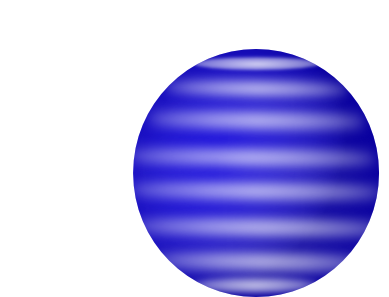
We have the conserved charges33 3 The link with the mathematics notation is: , , .:
| (3.1) |
They Poisson commute into a algebra. We can reparameterize the charges using the variable (where ):
| (3.2) |
The fundamental Poisson bracket reads .
3.1.2 The path integral
To better understand the path integral quantization procedure for the representations at hand, it will be useful to first perform a few explicit calculations with the discretized path integral for the finite dimensional representations. See e.g. [1][2]. We first discuss the calculation of the expectation value of the angular momentum and then that of the raising operator.
The angular momentum
In the quantum theory, it will be useful to add a total derivative term to the Lagrangian:
| (3.3) |
We use the variables which are the angle and the height parameter . The discretized path integral with insertion of the operator at a discrete point in time labelled by is then given by:
| (3.4) | |||||
We integrate over all discrete momenta , and over the intermediate positions , while specifying boundary conditions and on the path integral. We use the Haar measure. These finite dimensional integrals are straightforwardly computed:
| (3.5) |
To render the path integral periodic in the angular variable , we sum over all angles that differ by where . The term in the action proportional to the angle associates a phase to the winding sector labelled by . We obtain:
| (3.6) |
If we Fourier transform the initial condition and the final condition to dual integers and , we find that is equal to both. Indeed, the angular momentum is conserved over the course of the time evolution. We note that the angular momentum is an integer minus . We can therefore postulate that for unitary finite dimensional representations of with integer spin the parameter is zero, while for half-integer spin , the parameter is half-integer. This presupposes that the expression for the angular momentum is unmodified in the quantum theory. (See e.g. [1][2][11][15] for discussions of the parameter .)
The raising operator
We turn to the study of the action of the raising operator in the quantum theory. It is important to know when the raising operator annihilates a state, and therefore to resolve the quantum ambiguities in its definition, and in the choice of regularization. The path integral with an insertion of the raising operator at time can be discretized with a mid-point prescription as follows:
| (3.7) | |||||
with initial value and final condition . The integrals over the variables give rise to as many delta-functions. This leads to the constraints and . Thus, the path integral reduces to:
| (3.8) |
To get a periodic result, we again sum over final conditions where . This gives rise to:
We again Fourier transform the boundary conditions on the path integral:
The result is non-zero only when the initial and final angular momentum differ by one. Again, at integer spin , the parameter is zero, while at half-integer spin, it is half-integer. From standard representation theory, the expected coefficient for the action of the raising operator is:
| (3.9) |
We see that this agrees with our path integral result, with a definition for the raising operator which coincides with the classical operator (when using the mid-point prescription). From now on, we will assume that our quantization procedure agrees with the intuition that the classical vanishing of the raising operator indicates the appearance of a maximal vector in the quantum state space (with quantum eigenvalue just below the classical value).
3.2 The highest weight discrete representations
A path integral description of the quantum system with a Hilbert space consisting of a highest weight discrete representation with real highest weight lower than can also be constructed through the coadjoint orbit method applied to (see e.g. [16][15] and figure 2). The associated action is of the form:
| (3.10) |
where . Instead of integrating the coordinate from to , we integrate from to . For a given positive and a canonical choice of the parameter , the first eigenvalue of the angular momentum operator will be . Thus, the Hilbert space will be the highest weight representation of which is sometimes denoted as . Before we generalize this construction, we draw a few lessons.

Lessons
It should be clear that we can treat the finite dimensional and semi-infinite examples uniformly, by using the variables and to parameterize the phase space. The Poisson bracket of the position and momentum space variables is:
| (3.11) |
in both the above systems. We have a line segment or half-line with coordinate , and a circle bundle over it, with fiber parameterized by . The size of the circle fibered over the line segment depends on the point like on the interval , while it is equal to for points with parameter smaller than . In these variables, the algebra takes the form (up to a factor of ):
| (3.12) |
3.3 The Verma modules
We have reviewed the geometric path integral for spin for finite dimensional representations and certain highest weight representations. Our goal is to construct path integral formulations for more general representations. We first consider a positive integer and the highest weight representations . From the weight spaces of the Verma module it is clear that we can identify its phase space as consisting of the spherical phase space corresponding to a finite dimensional representation , combined with a hyperboloidal phase space of a Verma module (see figures 1, 2 and 3).

If we quantize the unified phase space as we did previously, with the action of the lowering and raising operators that we found before, then the space of states will take the direct sum form. We must make a modification such as to glue the two parts of the phase space into a Verma module . In particular, we must avoid the annihilation of the lowering operator at the bottom of the sphere.
To understand the gluing procedure, we first analyze a classical counterpart. If we suppose that the angular momentum generator still takes the form , then we have for any raising and lowering operator of the form that the Poisson bracket is satisfied. Let’s compute the bracket of two such charges:
| (3.13) |
For given solutions to the commutation relation , we have that any variation in which we multiply both by inverse functions will still satisfy the same Poisson bracket relations. Thus, to glue two representations, we rescale away the zero associated to the size of the circle fiber in either the raising or the lowering operator. In practice, we define the operators as:
| (3.14) |
We consider the path integral which consists of the two path integrals we described in subsections 3.1 and 3.2, but now we integrate over the full region of the variable . It should be clear that, first of all, the angular momentum spectrum will be the spectrum of the direct sum of the finite representation and the Verma module , since the range of integration of now covers both regions that previously gave rise to discretized angular momenta. The symmetry algebra is still realized. And, crucially, the lowering operator will not longer annihilate the state sitting at the bottom of the spherical part of the phase space (see figure 4).

We thus necessarily generate the desired representation . We can indeed check that the raising operator will still annihilate the top state in the representation, as well as the top state in the submodule . This follows from formula (3.9), and the fact that the raising operator in equation (3.14) gives rise to the coefficient (3.9) squared. This achieves the desired goal of a path integral realization of the Verma module .
An Invariant
We note that when we consider the algebra as realized in the direct sum representation, then the step function is an invariant. The step function Poisson-commutes with the charges in the direct sum (as in equation (3.12)) but not with the charges realizing the Verma module (as in equation (3.14)). This accords with intuition since the function assigns one value to one direct summand, and another to the second summand. This is not an invariant if we connect the two summands through the action of the algebra.
Analytic continuation
Finally we note that the operators (3.14) as well as the symplectic structure are analytic in (except at ). They allow for analytic continuation of our construction of Verma modules to all . At , the fixed point of the shifted Weyl reflection , the symplectic structure becomes singular. We treat this special case next.
3.4 The mock discrete representation
We can obtain the exceptional Verma module by quantizing the action:
| (3.15) |
We have the variable . The generators of take the form:
| (3.16) |
Quantizing as we did for finite or discrete highest weight representations (with ) gives rise to angular momenta (because of the choice of parameter and the range of integration of the coordinate – compare to equation (3.6)). The expression for the coefficient of the raising operator will now be – compare to equation (3.9) – which has a double zero. The lowering operator will have coefficient in terms of the same basis of states. This indeed gives rise to the Verma module , or equivalently, the mock discrete representation . This is an exceptional case since it does not arise from coadjoint orbit quantization. It can be obtained by a limiting procedure (in which one rescales both the variable as well as the charges ) from the Verma modules treated in subsection 3.3. The representation plays a special role due to the fact that its highest weight is self-mirror under Weyl reflection (shifted by half the sum of the positive roots).
3.5 The dual Verma modules
It is an easy exercise to show that the dual Verma modules as well are amenable to path integral quantization. It is sufficient to shift the zero from the raising to the lowering operator in the charges in equation (3.14).
3.6 The projective modules
We would like to extend the construction above to cover path integral realizations of the (non-trivial) projective modules of the BGG category . For the projective representations , where is a positive integer, one might expect a (partially) double-sheeted phase space corresponding to weight spaces of dimension two. However, within the projective representation, we would need to be able to move from one such sheet to the other. We need to quantize a geometry that incorporates this feature in its classical guise. Before we discuss this geometric realization, it will be useful to first study how projective representations arise in tensor product modules.
4 Multiplications
In this section, we study how various modules in the BGG category arise from more familiar modules, through the operation of taking tensor products. We will give explicit decomposition rules for some tensor product representations. Tensor products between finite and infinite dimensional modules have been studied in the mathematics literature (see e.g. [17, 18, 19]) but explicit formulas for decompositions of tensor products are hard to find. The decomposition rules can be obtained as in [20] from applying special projective functors to diagram algebras44 4 We would like to thank Catharina Stroppel for pointing this out. – here we follow a more pedestrian approach.
4.1 Tensoring finite dimensional modules
We start out with finite dimensional modules. Those all arise from taking consecutive tensor products of the two-dimensional representation with itself. We have the standard decomposition formula for spin:
| (4.1) |
4.2 Tensoring finite dimensional modules with Verma modules I
The next operation that we wish to study is the tensor product of finite dimensional representations with other indecomposable representations in the category . The result will always lie in the category . Let’s study the tensor product of a finite dimensional representation and an infinite dimensional highest weight representation, the Verma module . Since the tensor product operation is associative, and since all finite dimensional representations can be obtained by taking tensor products of the two-dimensional representation with itself, we can restrict our attention to the tensor product of the two-dimensional representation with a generic Verma module . We can decompose the result in terms of direct summands characterized by their character. A central element of the universal enveloping algebra will act on each such direct summand as a scalar character plus a nilpotent operator (see e.g. [8].
We moreover know [8] that the module permits a standard filtration (i.e. a filtration in terms of Verma modules) where the Verma modules arising as quotients are and . The weights are only linked when (i.e. these Verma modules can only combine into a non-direct sum representation when this condition is satisfied). In all other cases, the tensor product will be a direct sum of the two Verma modules. Note that for we have that is projective. Therefore, the tensor product with the finite dimensional representation will also be projective. The only possibility for the result of the tensor product is then the projective cover . We summarize:
| (4.2) |
We can summarize this in words by saying that any Verma modules appearing in the standard filtration of these tensor products that can team up will. Since we used some abstract nonsense to arrive at these results, it may be good to also demonstrate the non-trivial tensor product hands-on. In appendix B, we demonstrate through explicit calculation that these tensor product formulas hold.
It is clear now that to recursively compute tensor products of Verma modules with finite dimensional representations, we need to analyze the tensor product of projectives with finite dimensional modules first.
4.3 Tensoring finite dimensional with projective modules
We analyze the tensor product of the projective covers where with finite dimensional representations.
The basis for induction
We start out with the calculation of the tensor product . The result is necessarily projective, and therefore permits a filtration with Verma modules. By an analysis of the weight spaces, one sees that the standard filtration contains the Verma modules . These are linked two by two, namely and . The Verma module must appear as a factor in its projective cover , which is a direct summand. Generically, this is also true for the Verma module , which will appear in the summand . The only exception that can occur is when . In that case, we have that the Verma module is projective by itself. It then appears with multiplicity in the decomposition. We summarize:
| (4.3) |
Again, any Verma modules appearing in the standard filtration of the product that can link up must.
Notation
The following notation will be useful. For all , we define
| (4.4) |
where it is understood that the notation stands for the module with multiplicity two, . (This is an abusive notation that will be handy.) We can then compute the tensor product:
| (4.5) |
This can be checked on a case by case basis. The formula find its origin in the fact that Verma modules related by shifted Weyl reflection pair up in projective covers.
The induction step
We are now ready to prove the tensor product decomposition formula of projective modules with the finite dimensional representations. We claim the tensor product formula:
| (4.6) |
The basis for the induction was proven, namely, for arbitrary and for . Suppose now the formula holds for given and (as well as ). Then we tensor multiply on both sides of the decomposition formula. We use the decomposition as well as the fact that the formula holds for arbitrary and . We then subtract the result for from both sides. That proves the induction step, and therefore the tensor product decomposition formula (4.6).
4.4 Tensoring finite dimensional modules with Verma modules II
We turn to applying this insight to the tensor product of Verma modules with finite dimensional modules. Again we prove the decomposition formula by induction. For the induction hypothesis, we use the maxim that anything that can pair up, will (see figure 5). Consider the tensor product . It has a Verma module filtration with modules centered around . In order for a possibility for pairing to occur, we must have that either and , or and is amongst the highest weights of these Verma modules. Otherwise, we have a direct sum of Verma modules. When or are amongst these weights, the result will depend on whether is smaller than or bigger than . We propose:
| (4.7) | |||||
To prove this we use induction on . Suppose the induction step is true for (and smaller weights). Let’s continue the proof in a particular case. The other cases are proved analogously. Suppose that and even, and that is amongst the direct summands of . We have that the decomposition after tensoring in on the right hand side of the induction hypothesis (namely the second line of (4.7)) gives rise to the representations:
| (4.8) |
We then use the induction hypothesis (namely the third line of (4.7)) on the tensor product to take out the direct summands:
| (4.9) |
and we’re left with:
which proves the next step in the induction procedure.

4.5 Tensoring finite dimensional with dual Verma modules
The tensor product of finite dimensional modules with dual Verma modules is dual to the tensor product of finite dimensional modules with ordinary Verma modules. Thus, to obtain the tensor product decomposition formulas, we apply duality to the decomposition formulas we obtained before. Using that both projective and finite dimensional modules are self-dual, we get the desired result.
4.6 The path integral representation for projective modules
Since we have a path integral realization of the Verma modules and the finite dimensional modules in the category, it should be clear that their tensor product representations can be realized by taking products of the corresponding path integrals. Therefore, we now have in hand path integral representations for all (non-trivial) projective modules as well. For concreteness, we sketch the simplest example, in parallel to the discussion of the tensor product decomposition formulas. We start from the path integral representation of the Verma module (as in subsection 3.4) tensored with the path integral corresponding to the two-dimensional module (described in subsection 3.1). It is clear that the latter module will make sure that we can have two-dimensional weight spaces that are non-trivially interconnected in the quantum theory (see figure 6).

We now integrate over two variables and as well as two angle variables . The expressions for the charges are given by the sums:
| (4.10) |
We perform the path integral quantization with the action:
| (4.11) |
and due to the analysis of the factor path integrals given in subsections 3.1 and 3.4, the resulting phase space will correspond to the tensor product which we have proven to be equal to the projective representation . The other projective representations are found as direct summands in other tensor products that can also be obtained by product path integral quantizations. One can for instance isolate a given projective summand appearing in the tensor product of Verma modules with finite dimensional modules by projecting on a particular value of the quadratic Casimir squared.
Summary
For each module in the BGG category of representations, we have found a geometric system whose path integral quantization gives rise to that module.
5 Illustrations
In this section we discuss a few instances where the above representations appear in string theory. In subsection 5.1 we review a connection to the quantization of open strings ending on branes in a topological A-model, and discuss the representations that can be obtained in this context. In subsection 5.2 we discuss a particle model with reparameterization invariance that gives rise to a physical cohomology with features reminiscent of Berkovits cohomology on supercoset sigma-models.
5.1 Comparison to branes and quantization
In [11] a systematic approach to quantization was proposed using the topological A-model on a complexification of phase space admitting a complete hyper-Kähler metric. Essential ingredients are the canonical coisotropic brane [21][22] with support the whole of , as well as a Lagrangian A-brane . The Hilbert or vector space in the quantum theory consists of the strings, and the operators acting on them are obtained from strings which give rise to a non-commutative algebra of operators. These ideas are explained in detail in [11], where a comparison to other approaches to quantization is also made.
The main illustration of [11] is through the A-model on the Eguchi-Hanson space, viewed as the complexification of the two-sphere. It permits a natural action of . The classical equation for the two-sphere is translated into a constraint on the quadratic Casimir valid in the quantization of the algebra of polynomials in three variables . These variables satisfy the commutation relations in the quantum theory. Various choices of Lagrangian A-branes, as well as of parameters in the topological A-model, give rise to a host of representations of on the vector space of strings.
It is shown explicitly in [11] how finite dimensional representations can be associated to a brane wrapping a two-sphere, and how discrete representations arise from semi-infinite Lagrangian branes of cigar shape. It is also discussed how to glue two representations with semi-infinite spectra into a module with infinite spectrum, and that the quantization of branes can produce not only the principal unitary but also the complementary series representations (which are otherwise hard to access via geometric means).
Here, we propose an addendum to the discussion of [11]. Firstly, we remark that our construction of Verma modules (with positive integer ) should correspond to the quantization of spherical branes glued to semi-infinite Lagrangian branes, through turning on a vacuum expectation value for a string between these two branes with one given orientation. The dual Verma modules arise by turning on a vacuum expectation value for the string with opposite orientation. Turning on both expectation values would change the Casimir. This is very close to the discussion of the gluing of semi-infinite representations in [11]. Secondly, we remark that by taking the product of two spaces, and a diagonal algebra of strings, we are also able to produce the projective representations of from branes and their quantization, through the tensor product construction. Furthermore, in this way, we also have access to finite dimensional representations tensored with representations with infinite spectrum. This considerably extends the class of representations discussed both in [11] as well as in the bulk of this paper. All of them are geometrically accessible.
5.2 A reparameterization invariant particle model and its cohomology
Consider a particle living on the product of a hyperboloid (associated to a Verma module) and a sphere (associated to a finite dimensional representation). We define the action to be proportional to the total quadratic Casimir invariant (obtained for instance by taking the sums of charges appearing in the bulk of the paper, and forming the quadratic invariant). We can also add a mass term to the action. Thus, we can consider a reparameterization invariant action of the type (where is an einbein on the worldline of the particle). When we gauge fix reparameterization invariance (choosing ), we add a two-state ghost system to the theory. The BRST operator is then given by . In Siegel gauge, we will then have a cohomology made up of particles satisfying . Since is diagonalizable, we can compute the cohomology in the space of states satisfying . What happens next depends on the initial Casimirs and the mass. Either the space has only one dimensional weight spaces, and the states are in the cohomology. Or, some of the weight spaces are two-dimensional. In that case they will correspond to subspaces of projective representations. Then we will have that the operator maps one state to the other, and the other to zero. Thus, only the second state will be in the cohomology. A concrete example is the cohomology of in the space (times the two-state ghost system) which gives rise to a physical state space corresponding to the Verma module . In this example, we took the mass to be zero. Other examples are easily generated. The resulting cohomologies will generically project projective representations down to highest weight modules . Note that we can define a unitary norm on this phase space – it would not be invariant.
This construction is a simple analogue of the calculation of the cohomology for a reparameterization invariant particle on the supergroup [13]. The calculation is closely related due to the similarity in the action of the quadratic Casimir on the representation space.
A remark on the literature
In [23] a cohomology is defined with respect to the Casimir operator (minus the mass squared) itself. For instance, it is found that the cohomology of the quadratic Casimir on the space is the space . Indeed, the doubly degenerate weight spaces contain one exact and one non-closed state. Neither one is in the cohomology. One is left with the weight spaces of dimension one. The construction of [23] is thus quite different from the one we described above and from the calculation of the physical cohomology in certain reparameterization invariant string models [13].
6 Conclusions and suggestions
We provided a path integral description of generalized spin. Geometric models were proposed that after quantization give rise to all indecomposable representations in the BGG category of modules. In order to do so, we had to propose new models for Verma modules that do not belong to the unitary discrete series of , and provide the path integral realization of the generators of the algebra. To realize the projective representations we used product geometric spaces.
It would be very interesting to supply elementary models for all the brane quantizations described at the end of subsection 5.1, by explicitly combining the ingredients of this paper with those of [11]. It is then possible to give path integral realizations for all simple modules of (beyond category ). Also, although the category is considerably more complicated for algebras (and Casimirs) of higher rank, we are convinced that many of our ideas generalize to a large subset of the representations in those categories.
Acknowledgements
It is a pleasure to thank my colleagues and in particular Samuel Monnier and Catharina Stroppel for interesting discussions. My work was supported in part by the grant ANR-09-BLAN-0157-02.
Appendix A Descriptions
In this appendix we collect some useful details on modules in the BGG category . See [8] for further discussion.
A.1 The finite dimensional representation
The finite dimensional modules with a positive integer have dimension . We can choose basis vectors on which the algebra acts as:
| (A.1) |
The Casimir is a constant equal to . In standard physics notation the spin of this representation is equal to and the Casimir is then .
A.2 The Verma module
The Verma module can be defined as the module generated by the universal enveloping algebra acting on a highest weight vector with highest weight . The weights of the Verma module are . The explicit action of the generators on a basis consisting of vectors is given by the formulas:
| (A.2) |
Note that when is a positive integer, there will be another maximal vector (besides the vector ) inside the Verma module, namely the vector . In that case, the maximal submodule of the module is . The unique simple quotient of the module is then . When is not a positive integer the Verma module is simple. When the parameter is negative, the representation can be viewed as a discrete highest weight representation of , often denoted as , with highest weight and Casimir where .
A.3 The dual Verma module
Duality acting within the category maps the Verma module to its dual . The action of the algebra on basis vectors of the module can be computed via duality. First of all, duality preserves the weight spaces. We can therefore define a dual basis which consists of maps such that . Next, we wish to compute the action of the algebra on this dual vector space. The anti-involution used to define duality acts as: . The action of the generators on the dual basis then follows after a small calculation:
| (A.3) |
Note that when , we have that the basis vector is annihilated by the lowering operator . In that case, there is a non-trivial maximal submodule which is a . If we quotient the dual Verma module by the finite dimensional module , we obtain a module equivalent to the Verma module . This illustrates the fact that duality inverts short exact sequences.
A.4 The projective module
The projective module for a positive integer has weights with multiplicity one, and the weights with multiplicity two. We can choose the action on the weight vectors and to be:
| (A.4) |
We have a Verma submodule , as well as a Verma submodule . It is interesting to compute the action of the quadratic Casimir on the projective representation . The action on the vectors will be diagonal and equal to the constant . The action on the vectors however is equal to:
| (A.5) |
This is neither diagonal nor diagonalizable. If we act with the operator we will find zero. The quadratic Casimir has two-by-two Jordan block structure in the eigenspaces with eigenvalues
Appendix B Decompositions
Let’s analyze the action of the quadratic Casimir in the tensor product space :
One of the last two terms is necessarily zero. Indeed, we have the actions and . On the maximal vector the Casimir acts diagonally with factor . Now we study the level one below. It contains a maximal vector (by the fact that the level above is one-dimensional). Let’s compute the matrix of the action of the Casimir on the vectors and . We obtain:
| (B.1) |
The matrix has a characteristic polynomial with zeros , which are the generalized eigenvalues of the quadratic Casimir. When the eigenvalues are not equal, the matrix is diagonalizable. Due to the structure of the weight space, we then identify two direct summands in the tensor product which are the Verma modules and . On the other hand, the eigenvalues are equal when . In this case, the action of the quadratic central element becomes:
which is equivalent to:
The fact that the action is not diagonalizable demonstrates that we deal with a projective module, which due to the structure of the weight spaces must be . This can be seen a little more explicitly by identifying and as two highest weight vectors, and noting that the top state can be reached from the a non-highest weight vector at the level below. This illustrates the indecomposable nature of the module, and its non-trivial standard filtration in terms of modules and . As a side remark, we note the similarity between the action of the raising and lowering operators on the weight spaces of weight and , and the action of fermionic generators within projective representations of (see e.g. [24]). This similarity in the end leads to an isomorphic action of the quadratic Casimir on weight spaces. (See also subsection 5.2.)
References
- [1] H. Nielsen and D. Rohrlich, “A Path Integral To Quantize Spin,” Nucl. Phys. B 299 (1988) 471.
- [2] K. Johnson, “Functional Integrals For Spin,” Annals Phys. 192 (1989) 104.
- [3] A. Alekseev, L. Faddeev and S. Shatashvili, “Quantization of symplectic orbits of compact Lie groups by means of the functional integral,” J. Geom. Phys. 5 (1988) 391.
- [4] B. Kostant, Quantization and unitary representations, Modern Analysis and Applications, Lecture Notes in Math., Vol. 170, pp. 87-207. Berlin-Heidelberg-New York, Springer 1970.
- [5] J. Souriau, Structure des systèmes dynamiques, Paris, Dunod, 1970.
- [6] N. Woodhouse, Geometric quantization, New York, Clarendon, 1992.
- [7] A. Kirillov, Lectures on the orbit method, Graduate Studies in Mathematics 64, American Mathematical Society, Providence, RI, 2004.
- [8] J. Humphreys, Representations of Semisimple Lie Algebras in the BGG Category O, Grad. Stud. Math., 94, Amer. Math. Soc., Providence, RI, 2008.
- [9] Y. Satoh, “Three point functions and operator product expansion in the SL(2) conformal field theory,” Nucl. Phys. B 629 (2002) 188 [hep-th/0109059].
- [10] J. Maldacena and H. Ooguri, “Strings in AdS(3) and the SL(2,R) WZW model. Part 3. Correlation functions,” Phys. Rev. D 65 (2002) 106006 [hep-th/0111180].
- [11] S. Gukov and E. Witten, “Branes and Quantization,” arXiv:0809.0305 [hep-th].
- [12] G. Gotz, T. Quella and V. Schomerus, “The WZNW model on ,” JHEP 0703 (2007) 003 [hep-th/0610070].
- [13] J. Troost, “Massless particles on supergroups and supergravity,” JHEP 1107 (2011) 042 [arXiv:1102.0153 [hep-th]].
- [14] M. R. Gaberdiel and S. Gerigk, “The massless string spectrum on from the supergroup,” JHEP 1110 (2011) 045 [arXiv:1107.2660 [hep-th]].
- [15] J. Troost and A. Tsuchiya, “Three-dimensional black hole entropy,” JHEP 0306 (2003) 029 [hep-th/0304211].
- [16] E. Witten, “Coadjoint Orbits of the Virasoro Group,” Commun. Math. Phys. 114 (1988) 1.
- [17] B. Kostant, “On the tensor product of a finite and an infinite dimensional representation”, Journal of Functional Analysis 20, 4 (1975), 257-285.
- [18] G. Zuckerman, “Tensor products of finite and infinite dimensional representations of semisimple Lie groups”, Annals of Mathematics 106 (1977), 295-308.
- [19] J. Bernstein and S. Gelfand, “Tensor products of finite and infinite dimensional representations of semisimple Lie algebras”, Compositio Mathematica 41, 2 (1980), 245-285.
- [20] J. Brundan and C. Stroppel, “Highest weight categories arising from Khovanov’s diagram algebra III: category O”, Represent. Theory 15 (2011), 170-243
- [21] A. Kapustin and D. Orlov, “Remarks on A branes, mirror symmetry, and the Fukaya category,” J. Geom. Phys. 48 (2003) 84 [hep-th/0109098].
- [22] A. Kapustin and E. Witten, “Electric-Magnetic Duality And The Geometric Langlands Program,” hep-th/0604151.
- [23] A. van Tonder, “Cohomology and decomposition of tensor product representations of SL(2,R),” Nucl. Phys. B 677 (2004) 614 [hep-th/0212149].
- [24] V. Schomerus and H. Saleur, “The WZW model: From supergeometry to logarithmic CFT,” Nucl. Phys. B 734 (2006) 221 [hep-th/0510032].