跳到论文正文
W Papers独立论文阅读器 arXiv:1202.1912 论文正文 计算阅读时间 · 0%
引用这篇论文根据当前论文元数据生成,正式投稿前建议核对。


License: arXiv.org perpetual non-exclusive license
arXiv:1202.1912v1 [hep-th] 09 Feb 2012

The No-Pole Condition in Landau gauge:
Properties of the Gribov Ghost Form-Factor
and a Constraint on the 2​d2d Gluon Propagator

Attilio Cucchieri Email: attilio@ifsc.usp.br Affiliation: Ghent University, Department of Physics and Astronomy, Krijgslaan 281-S9,
9000 Gent, Belgium
Affiliation: Instituto de Física de São Carlos, Universidade de São Paulo, Caixa Postal 369,
13560-970 São Carlos, SP, Brazil
   David Dudal Email: david.dudal@ugent.be Affiliation: Ghent University, Department of Physics and Astronomy, Krijgslaan 281-S9,
9000 Gent, Belgium
   Nele Vandersickel Email: nele.vandersickel@ugent.be Affiliation: Ghent University, Department of Physics and Astronomy, Krijgslaan 281-S9,
9000 Gent, Belgium
Abstract

We study general properties of the Landau-gauge Gribov ghost form-factor σ⁡(p2)\sigma(p^{2}) for SU(NcN_{c}) Yang-Mills theories in the dd-dimensional case. We find a qualitatively different behavior for d=3,4d=3,4 with respect to the d=2d=2 case. In particular, considering any (sufficiently regular) gluon propagator 𝒟⁡(p2)\mathcal{D}(p^{2}) and the one-loop-corrected ghost propagator, we prove in the 2​d2d case that the function σ⁡(p2)\sigma(p^{2}) blows up in the infrared limit p→0p\to 0 as −𝒟⁡(0)​ln⁡(p2)-\mathcal{D}(0)\ln(p^{2}). Thus, for d=2d=2, the no-pole condition σ⁡(p2)<1\sigma(p^{2})<1 (for p2>0p^{2}>0) can be satisfied only if the gluon propagator vanishes at zero momentum, that is, 𝒟⁡(0)=0\mathcal{D}(0)=0. On the contrary, in d=3d=3 and 4, σ⁡(p2)\sigma(p^{2}) is finite also if 𝒟⁡(0)>0\mathcal{D}(0)>0. The same results are obtained by evaluating the ghost propagator 𝒢⁡(p2)\mathcal{G}(p^{2}) explicitly at one loop, using fitting forms for 𝒟⁡(p2)\mathcal{D}(p^{2}) that describe well the numerical data of the gluon propagator in two, three and four space-time dimensions in the SU(2) case. These evaluations also show that, if one considers the coupling constant g2g^{2} as a free parameter, the ghost propagator admits a one-parameter family of behaviors (labelled by g2g^{2}), in agreement with previous works by Boucaud et al. In this case the condition σ⁡(0)≤1\sigma(0)\leq 1 implies g2≤gc2g^{2}\leq g^{2}_{c}, where gc2g^{2}_{c} is a “critical” value. Moreover, a free-like ghost propagator in the infrared limit is obtained for any value of g2g^{2} smaller than gc2g^{2}_{c}, while for g2=gc2g^{2}=g^{2}_{c} one finds an infrared-enhanced ghost propagator. Finally, we analyze the Dyson-Schwinger equation for σ⁡(p2)\sigma(p^{2}) and show that, for infrared-finite ghost-gluon vertices, one can bound the ghost form-factor σ⁡(p2)\sigma(p^{2}). Using these bounds we find again that only in the d=2d=2 case does one need to impose 𝒟⁡(0)=0\mathcal{D}(0)=0 in order to satisfy the no-pole condition. The d=2d=2 result is also supported by an analysis of the Dyson-Schwinger equation using a spectral representation for the ghost propagator. Thus, if the no-pole condition is imposed, solving the d=2d=2 Dyson-Schwinger equations cannot lead to a massive behavior for the gluon propagator. These results apply to any Gribov copy inside the so-called first Gribov horizon, i.e. the 2​d2d result 𝒟⁡(0)=0\mathcal{D}(0)=0 is not affected by Gribov noise. These findings are also in agreement with lattice data.

I Introduction

Green functions of Yang-Mills theories are gauge-dependent quantities. They can, however, be used as a starting point for the evaluation of hadronic observables (see for example [1, 2, 3, 4]). Thus, the study of the infrared (IR) behavior of propagators and vertices is an important step in our understanding of QCD. In particular, the confinement mechanism for color charges [5] could reveal itself in the IR behavior of (some of) these Green functions. This IR behavior should also be relevant for the description of the deconfinement transition and of the deconfined phase of QCD. Indeed, at high temperature color charges are expected to be Debye-screened and the (electric and magnetic) screening masses should be related to the IR behavior of the gluon propagator (see for example [6, 7, 8]).

Among the gauge-fixing conditions employed in studies of Yang-Mills Green functions, a very popular choice is the Landau gauge, which in momentum space reads pμ​Aμb​(p)=0p_{\mu}A_{\mu}^{b}(p)=0. From the continuum perspective this gauge has various important properties, including its renormalizability, various associated nonrenormalization theorems [9] and a ghost-antighost symmetry [1]. In the past few years many analytic studies of Green functions in Landau gauge have focused on the solution of the Yang-Mills Dyson-Schwinger equations (DSEs), which are the exact quantum equations of motion of the theory (see for example [1, 2, 10, 11]). Since the DSEs are an infinite set of coupled equations, any attempt of solving them requires a truncation scheme. Then, some Green functions (usually the gluon and the ghost propagators) are obtained self-consistently from the considered equations, while all the other Green functions entering the equations are given as an input. For the coupled DSEs of gluon and ghost propagators two solutions have been extensively analyzed (see for example Chapter 10 in Ref. [5] and Ref. [12] for recent short reviews). The scaling solution [1, 13, 14, 15, 16] finds in d=2,3d=2,3 and 4 an IR-enhanced ghost propagator 𝒢⁡(p2)\mathcal{G}(p^{2}) and a vanishing gluon propagator 𝒟⁡(p2)\mathcal{D}(p^{2}) at zero momentum.11 1 For the explanation of color confinement based on the scaling solution see for example Section 3.4 in [17] and references therein. In particular, the IR behavior of the two propagators should be given respectively by 𝒢⁡(p2)∼(p2)−κG−1\mathcal{G}(p^{2})\sim(p^{2})^{-\kappa_{G}-1} and by 𝒟⁡(p2)∼(p2)2​κD+(2−d)/2\mathcal{D}(p^{2})\sim(p^{2})^{2\kappa_{D}+(2-d)/2} with κG=κD≈0.2​(d−1)\kappa_{G}=\kappa_{D}\approx 0.2(d-1) [14, 16]. On the other hand, the massive solution [18, 19, 20, 21, 22, 23, 24, 25, 26] gives (for d=3d=3 and 4) a free-like ghost propagator in the IR limit, i.e. κG=0\kappa_{G}=0, and a massive behavior for the gluon propagator,22 2 The possible existence of a dynamical mass for the gluons, as well as its relation to quark confinement through vortex condensation, has been discussed a long time ago in Ref. [27]. that is, 𝒟⁡(0)>0\mathcal{D}(0)>0 and κD=(d−2)/4\kappa_{D}=(d-2)/4.

The existence of two different types of solution for the coupled gluon and ghost DSEs is now understood as due to the use of different auxiliary boundary conditions.33 3 The possibility of having different non-perturbative solutions for DSEs in relation with different boundary conditions has been discussed for example in Refs. [28, 29] (see also Section 1.4 in [30] and Sections 3 and 3.1 in Ref. [1]). These conditions can be given in terms of the value of the ghost dressing function ℱ⁡(p2)=p2​𝒢​(p2)\mathcal{F}(p^{2})=p^{2}\mathcal{G}(p^{2}) at a given momentum scale pp [22, 31]. In particular, if one considers p=0p=0, it is clear that 1/ℱ⁡(0)=01/\mathcal{F}(0)=0 gives an IR-enhanced ghost propagator 𝒢⁡(p2)\mathcal{G}(p^{2}) while 1/ℱ⁡(0)>01/\mathcal{F}(0)>0 yields a free-like behavior for 𝒢⁡(p2)\mathcal{G}(p^{2}) at small momenta. As stressed in Ref. [22] (see also the discussion in Section 4.2.2 of Ref. [12]), the scaling condition 1/ℱ⁡(0)=01/\mathcal{F}(0)=0 relies on a particular cancellation in the ghost DSE which, in turn, implies a specific “critical” value gc2g^{2}_{c} for the coupling constant g2g^{2} [12, 32]. Thus, at least from the mathematical point of view, there is a one-parameter family of solutions for the gluon and ghost DSEs, labelled by g2g^{2} or, equivalently, by 1/ℱ⁡(0)1/\mathcal{F}(0): in the case g2=gc2g^{2}=g^{2}_{c} one recovers the scaling solution while, for all cases g2<gc2g^{2}<g^{2}_{c}, the solution is a massive one.44 4 If g2>gc2g^{2}>g^{2}_{c} one gets a negative ghost propagator at small momenta. In 4​d4d, the SU(3) physical value of the coupling seems to select55 5 Recently, in Ref. [33], it has also been shown — using a renormalization-group approach — that in three and four space-time dimensions only the decoupling solution is expected to be physically realized. the massive solution [21, 34].

At this point we should recall that, when considering gauge-dependent quantities in non-Abelian gauge theories, one has to deal with the existence of Gribov copies [35] (see also Ref. [36] for a recent review). Indeed, for compact non-Abelian Lie groups defined on the 4-sphere [37] or on the 4-torus [38], it is impossible to find a continuous choice of one (and only one) connection Aμ​(x)A_{\mu}(x) on each gauge orbit. The effect of Gribov copies is not seen in perturbation theory [35], i.e. the usual Faddeev-Popov-quantization procedure is correct at the perturbative level. However, these copies could be relevant at the non-perturbative level, i.e. in studies of the IR properties of Yang-Mills theories.

Different approaches have been proposed in order to quantize a Yang-Mills theory while taking into account the existence of Gribov copies (see for example [35, 39, 40, 41, 43, 42, 44, 45]). The one usually considered, both in the continuum and on the lattice, is based on restricting the functional integration to a subspace of the hyperplane of transverse configurations. The original proposal, made by Gribov [35], was based on the observation that the Landau gauge condition ∂μAμb​(x)=0\partial_{\mu}A_{\mu}^{b}(x)=0 allows for (infinitesimally) gauge-equivalent configurations if the Landau-gauge Faddeev-Popov operator ℳb​c(x,y)=−δ(x−y)∂μDμb​c\mathcal{M}^{bc}(x,y)=-\delta(x-y)\partial_{\mu}D_{\mu}^{bc} has zero modes. (Here Dμb​cD_{\mu}^{bc} is the usual covariant derivative.) Indeed, since an infinitesimal gauge transformation δ​ω​(x)\delta\omega(x) gives Aμb​(x)→Aμb​(x)+Dμb​c​ωc​(x)A_{\mu}^{b}(x)\to A_{\mu}^{b}(x)+D_{\mu}^{bc}\omega^{c}(x), it is clear that the exclusion (in the path-integral measure) of the zero modes of ℳb​c​(x,y)\mathcal{M}^{bc}(x,y) implies that gauge copies connected by such infinitesimal gauge transformations are ignored in the computation of expectation values. In order to exclude these zero modes, Gribov considered a stronger condition by requiring that the functional integration be restricted to the region Ω\Omega of gauge configurations Aμb​(x)A^{b}_{\mu}(x) defined as

Ω≡{Aμb(x):∂μAμb(x)=0,ℳb​c(x,y)>0}.\Omega\,\equiv\,\left\{\,A^{b}_{\mu}(x):\;\partial_{\mu}A^{b}_{\mu}(x)=0\;,\;\mathcal{M}^{bc}(x,y)>0\right\}\;. (1)

This set, known as the (first) Gribov region, clearly includes the vacuum configuration Aμb​(x)=0A^{b}_{\mu}(x)=0, for which the Faddeev-Popov operator is given by −δ(x−y)δb​c∂μ2-\delta(x-y)\delta^{bc}\partial_{\mu}^{2}. The region Ω\Omega can also be defined (see for example [46, 47]) as the whole set of local minima66 6 For this reason this gauge condition is often indicated in the literature as minimal Landau gauge. of the functional ℰ⁡[A]=∫dd​x​Aμb​(x)​Aμb​(x)\mathcal{E}[A]\,=\,\int\,\mathrm{d}^{d}x\,A_{\mu}^{b}(x)\,A_{\mu}^{b}(x). Since usually each orbit allows for more than one local minimum of ℰ⁡[A]\mathcal{E}[A], it is clear that the region Ω\Omega is not free of Gribov copies. On the contrary, in the interior of the so-called fundamental modular region Λ\Lambda, given by the set of the absolute minima of the functional ℰ⁡[A]\mathcal{E}[A], no Gribov copies occur [43, 48].

The characterization of the fundamental modular region Λ\Lambda, i.e. finding the absolute minima of the energy functional ℰ⁡[A]\mathcal{E}[A], is a problem similar to the determination of the ground state of a spin glass system [49, 50]. Thus, a local formulation of a Yang-Mills theory, with the functional measure delimited to Λ\Lambda, is not available, whereas a practical way of restricting the physical configuration space to the region Ω\Omega was introduced by Gribov [35]. To this end, he required that the ghost dressing function ℱ⁡(p2)\mathcal{F}(p^{2}) cannot have a pole at finite nonzero momenta. After setting

𝒢⁡(p2)=ℱ⁡(p2)p2=1p2​11−σ⁡(p2),\mathcal{G}(p^{2})\,=\,\frac{\mathcal{F}(p^{2})}{p^{2}}\,=\,\frac{1}{p^{2}}\frac{1}{1-\sigma(p^{2})}\;, (2)

this condition can be written as

σ⁡(p2)​<1forp2>​0,\sigma(p^{2})<1\qquad\mbox{for}\qquad p^{2}>0\;, (3)

where σ⁡(p2)\sigma(p^{2}) is the so-called Gribov ghost form-factor [35]. Indeed, since the ghost propagator is given by

𝒢⁡(p2)=δb​cNc2−1​⟨p​|(ℳ−1)b​c|​p⟩,\mathcal{G}(p^{2})\,=\,\frac{\delta^{bc}}{N^{2}_{c}-1}\,\left<\,p\,\left|\,\left(\mathcal{M}^{-1}\right)^{bc}\,\right|\,p\,\right>\;, (4)

i.e. it is related to the inverse of the Faddeev-Popov matrix ℳb​c​(x,y)\mathcal{M}^{bc}(x,y), the above inequality — known as the no-pole condition — should be equivalent to the restriction of the functional integration to the Gribov region Ω\Omega, i.e. to the condition ℳb​c​(x,y)>0\mathcal{M}^{bc}(x,y)>0.

From the discussion above, it is clear that both scaling and massive solutions of DSEs satisfy the no-pole condition, i.e. 1/ℱ⁡(p2)=1−σ⁡(p2)>01/\mathcal{F}(p^{2})=1-\sigma(p^{2})>0 for p2>0p^{2}>0. Indeed, in the scaling case [1, 13, 14, 15, 16], this condition [together with the condition 1/ℱ⁡(0)=01/\mathcal{F}(0)=0] is imposed from the beginning to the solution of the DSEs. On the contrary, for the massive solution, the no-pole condition is either verified a posteriori, as in Ref. [20], or used [together with the condition 1/ℱ⁡(0)>01/\mathcal{F}(0)>0] as an input for the solution of the DSEs, as in Refs. [19, 25, 26]. In particular, in Ref. [26], the value of 1/ℱ⁡(0)1/\mathcal{F}(0) is fixed using lattice data.

The restriction to the first Gribov region Ω\Omega is also always implemented in lattice numerical simulations of Green functions in Landau gauge by (numerically) finding local minima of the functional ℰ⁡[A]\mathcal{E}[A]. Results obtained using very large lattice volumes [51, 52, 53, 54] (see also Chapter 10 in Ref. [5], Section 3 in Ref. [12] and Ref. [55] for recent short reviews) have shown that in d=3d=3 and 4 the gluon propagator 𝒟⁡(p2)\mathcal{D}(p^{2}) is finite and nonzero in the limit p→0p\to 0 while the ghost propagator 𝒢⁡(p2)\mathcal{G}(p^{2}) behaves as 1/p21/p^{2}. On the contrary, for d=2d=2 the lattice data [56, 57, 58, 59] are in quantitative agreement with the scaling solution and one finds κD=κG≈0.2\kappa_{D}=\kappa_{G}\approx 0.2.

Since the region Ω\Omega is not free of Gribov copies, their (possible) influence on the numerical evaluation of gluon and ghost propagators has been studied by various groups [61, 62, 63, 64, 65, 66]. It has been found that these effects are usually observable only the IR limit and that any attempt to restrict the functional integration to the fundamental modular region Λ\Lambda gives a stronger suppression at small momenta for both propagators, i.e. reducing the value of 𝒟⁡(0)\mathcal{D}(0) and increasing that of 1/ℱ⁡(0)1/\mathcal{F}(0). More recently, it has been suggested [67, 68, 69, 70] that the one-parameter family of solutions obtained for the gluon and ghost DSEs should be related77 7 This identification is, however, based on several (unproven) hypotheses, as already stressed in Ref. [58]. to Gribov-copy effects and that the value of 1/ℱ⁡(0)1/\mathcal{F}(0) could be used as a gauge-fixing parameter. This analysis finds indeed IR-enhanced ghost propagators (and sometimes a disconcerting over-scaling88 8 Let us recall that the scaling solution is supposed to be unique [31].). On the other hand, the gluon propagator still shows a finite nonzero value at zero momentum, that is, 𝒟⁡(0)>0\mathcal{D}(0)>0. Moreover, this approach does not explain why the numerical results found in d=2d=2 are different from those obtained in d=3d=3 and 4, even though Gribov copies inside the first Gribov region Ω\Omega are clearly present in any space-time dimension d>1d>1.

From the analytical point of view, following Gribov’s approach, Zwanziger modified the usual Yang-Mills action in order to restrict the path integral to the first Gribov region Ω\Omega [71] Although this restriction is obtained using a non-local term, the Gribov-Zwanziger (GZ) action99 9 See again Ref. [36] for a comprehensive review of the GZ action. can be written as a local action and it is proven [72, 73, 74] to be renormalizable. At tree level the GZ gluon propagator is given by 𝒟⁡(p2)=p2/(p4+λ4)\mathcal{D}(p^{2})=p^{2}/(p^{4}+\lambda^{4}), where λ\lambda is a parameter with mass-dimension 1. At the same time, the ghost propagator is given by 𝒢⁡(p2)∼1/p4\mathcal{G}(p^{2})\sim 1/p^{4}. Thus, as in the scaling solution of the gluon and ghost DSEs, the gluon propagator is null at zero momentum1010 10 One can, however, obtain a finite nonzero value for 𝒟⁡(0)\mathcal{D}(0) within the GZ approach by considering a non-analytic behavior for the free energy of the system [75, 76]. and the ghost propagator is IR-enhanced [42]. These tree-level results, also in agreement with the original work by Gribov [35], have been confirmed by one-loop calculations in the three- and four-dimensional cases [77, 78, 79, 80, 81].

More recently, the GZ action has been modified by considering (for d=3d=3 and 4) dimension-two condensates [82, 83, 84, 85]. The corresponding action, called the Refined Gribov-Zwanziger (RGZ) action, still imposes the restriction of the functional integration to the region Ω\Omega and it is renormalizable. However, the RGZ action allows for a finite nonzero value of 𝒟⁡(0)\mathcal{D}(0) and for a free-like ghost propagator 𝒢⁡(p2)\mathcal{G}(p^{2}) in the IR limit. Thus, nonzero values for these dimension-two condensates yield for the gluon and ghost propagators an IR behavior in agreement with the massive solution of the gluon and ghost DSEs.1111 11 Let us note here that a massive behavior for these two propagators has also been obtained in Refs. [86, 87] using different analytic approaches. Indeed, the RGZ tree-level gluon propagator describes well the numerical data in the SU(2) case [59, 60], for d=3d=3 and 4, and in the SU(3) case [88] with d=4d=4. It is also interesting to note that the fitting values for the dimension-two condensates are very similar for the SU(2) and SU(3) gauge groups in the four-dimensional case.

As stressed above, the restriction of the functional integration to the first Gribov region Ω\Omega and the no-pole condition (3) are key ingredients in the study of the IR sector of Yang-Mills theories in Landau gauge. However, to our knowledge, a detailed investigation of the properties of the Gribov form-factor σ⁡(p2)\sigma(p^{2}) as well as of the possible implications of the no-pole condition was missing up to now, although some interesting one-loop results were already presented in Refs. [84, 89, 90, 91]. In particular, in Appendix B.2 of [84] it was shown that, if the gluon propagator 𝒟⁡(p2)\mathcal{D}(p^{2}) is positive, then in the 2​d2d case the derivative ∂σ⁡(p2)/∂p2\partial\sigma(p^{2})/\partial p^{2} is negative for all values of p2p^{2}, i.e. σ⁡(p2)\sigma(p^{2}) is largest at p2=0p^{2}=0. Also, in Ref. [89] it was proven that in the RGZ framework the form-factor σ⁡(p2)\sigma(p^{2}) presents a logarithmic IR singularity −ln⁡(p2)-\ln(p^{2}) for d=2d=2. This result precluded the use of the RGZ action in the two-dimensional case, leading to a first interpretation of the different behavior found in lattice numerical simulations for the 2​d2d case, compared to the d=3d=3 and 4 cases. Similar findings have been (more recently) presented in Refs. [33, 92, 93].

In this work we collect some general properties of the Gribov form-factor σ⁡(p2)\sigma(p^{2}) and we study the consequences of imposing the no-pole condition. In particular, in Section II, using the expression for σ⁡(p2)\sigma(p^{2}) obtained from the evaluation of the ghost propagator at one loop, we prove that σ⁡(p2)\sigma(p^{2}) attains its maximum value at p2=0p^{2}=0 for any dimension d≥2d\geq 2. Since this expression for σ⁡(p2)\sigma(p^{2}) depends on the gluon propagator 𝒟⁡(p2)\mathcal{D}(p^{2}), in the same section we also investigate (for a general dd-dimensional space-time) which IR behavior of the gluon propagator is necessary in order to satisfy the no-pole condition σ⁡(p2)<1\sigma(p^{2})<1. By considering a generic (and sufficiently regular) gluon propagator 𝒟⁡(p2)\mathcal{D}(p^{2}), we find in the d=2d=2 case that σ⁡(p2)\sigma(p^{2}) is unbounded unless the gluon propagator is null at zero momentum. More exactly, we find σ⁡(p2)∼−𝒟⁡(0)​ln⁡(p2)\sigma(p^{2})\sim-\mathcal{D}(0)\ln(p^{2}) in the p→0p\to 0 limit, in agreement with [89]. This result does not apply to the d=3d=3 and 4 cases. Indeed, in these cases one can introduce, for all values of p2p^{2}, simple finite upper bounds for the Gribov form-factor. In Section III we present explicit one-loop calculations for σ⁡(p2)\sigma(p^{2}) using for the gluon propagator 𝒟⁡(p2)\mathcal{D}(p^{2}) linear combinations of Yukawa-like propagators (with real and/or complex-conjugate poles), which have been recently used to model lattice data of the gluon propagator in the SU(2) case [59, 60]. Besides confirming the results obtained in Section II, we also find that the ghost propagator admits a one-parameter family of behaviors [21] labelled by the coupling constant g2g^{2}, considered as a free parameter. Moreover, the massive solution 𝒢⁡(p2)∼1/p2\mathcal{G}(p^{2})\sim 1/p^{2}, corresponding to σ⁡(0)<1\sigma(0)<1, is obtained for all values of g2g^{2} smaller than a “critical” value gc2g^{2}_{c}. At the “critical” value gc2g^{2}_{c}, implying σ⁡(0)=1\sigma(0)=1, one finds an IR-enhanced ghost propagator. (As already stressed above, the case g2>gc2g^{2}>g^{2}_{c} corresponds to σ⁡(0)>1\sigma(0)>1 and one obtains a negative ghost propagator at small momenta.) Finally, in Section IV, we analyze the DSE for σ⁡(p2)\sigma(p^{2}). We stress that in this case we do not try to solve the DSE but we focus only on general properties of this equation. As we will see, considering IR-finite ghost-gluon vertices, we confirm and extend the one-loop analysis of the no-pole condition presented in Section II. In particular, after introducing bounds for the Gribov form-factor, we show again for d=2d=2 that the gluon propagator 𝒟⁡(p2)\mathcal{D}(p^{2}) must vanish at zero momentum in order to keep σ⁡(p2)\sigma(p^{2}) finite. On the contrary, such a constraint does not apply in the three- and four-dimensional cases. We also present alternative evidence for the d=2d=2 result using a spectral representation for the ghost propagator in the DSE.

It is important to note that all our results in Sections II and IV apply irrespective of which set of Gribov copies (inside the region Ω\Omega) is considered, i.e. they are not affected by the so-called Gribov noise. We end with our Conclusion in Section V. Some technical details have been collected in four Appendices. In particular, in Appendix B we present properties of the Gauss hypergeometric function F12​(a,b,c,z){}_{2}F_{1}\left(a,b;c;z\right) that are relevant to prove some of our results.

Refer to caption
Figure 1: Feynman diagrams for the one-loop-corrected Landau-gauge ghost propagator. Dashed lines represent ghosts, the curly line represents gluons.

II The One-Loop-Corrected Ghost Propagator and the Gribov Form-Factor

In this Section, as well as in Section III below, we consider the one-loop-corrected Landau-gauge ghost propagator, diagrammatically represented in Figure 1. This propagator can be written [for the SU(NcN_{c}) gauge group in the dd-dimensional case] as

𝒢⁡(p2)=1p2−δa​bNc2−1​1p4​g2​fa​d​c​fc​d​b​∫dd​q(2​π)d​(p−q)μ​pν​𝒟​(q2)​Pμ​ν​(q)​1(p−q)2,\mathcal{G}(p^{2})\,=\,\frac{1}{p^{2}}\,-\,\frac{\delta^{ab}}{N_{c}^{2}-1}\,\frac{1}{p^{4}}\,g^{2}f^{adc}f^{cdb}\int\frac{\mathrm{d}^{d}q}{(2\pi)^{d}}\,(p-q)_{\mu}\,p_{\nu}\,\mathcal{D}(q^{2})\,P_{\mu\nu}(q)\,\frac{1}{(p-q)^{2}}\;, (5)

where δa​b​𝒟​(q2)​𝒫μ​ν​(q)\delta^{ab}\,\mathcal{D}(q^{2})\,\mathcal{P}_{\mu\nu}(q) is the tree-level gluon propagator [not necessarily given by 𝒟⁡(q)=1/q2\mathcal{D}(q)=1/q^{2}] and 𝒫μ​ν​(q)=(δμ​ν−qμ​qν/q2)\mathcal{P}_{\mu\nu}(q)=\left(\delta_{\mu\nu}-q_{\mu}q_{\nu}/q^{2}\right) is the usual projector onto the transverse sub-space, i.e. qμ​𝒫μ​ν​(q)=0q_{\mu}\mathcal{P}_{\mu\nu}(q)=0. We have also considered the tree-level ghost-gluon vertex i​g​fa​d​c​pν\,igf^{adc}p_{\nu}, where pp is the outgoing ghost momentum. The indices a,d,ca,d,c refer, respectively, to the incoming ghost, to the gluon and to the outcoming ghost. After using fa​d​c​fc​d​b=−Nc​δa​bf^{adc}\,f^{cdb}=-N_{c}\delta^{ab}, valid for the adjoint representation, we obtain

𝒢⁡(p2)=1p2​[ 1+σ⁡(p2)],\mathcal{G}(p^{2})\,=\,\frac{1}{p^{2}}\,\left[\,1\,+\,\sigma(p^{2})\,\right]\;, (6)

where σ⁡(p2)\sigma(p^{2}) is the momentum-dependent function

σ⁡(p2)=g2​Nc​pμ​pνp2​∫dd​q(2​π)d​1(p−q)2​𝒟​(q2)​𝒫μ​ν​(q).\sigma(p^{2})\,=\,g^{2}N_{c}\frac{p_{\mu}p_{\nu}}{p^{2}}\int\frac{\mathrm{d}^{d}q}{(2\pi)^{d}}\frac{1}{(p-q)^{2}}\mathcal{D}(q^{2})\,\mathcal{P}_{\mu\nu}(q)\;. (7)

Finally, we can write [as in Eq. (2)]

𝒢⁡(p2)=1p2​11−σ⁡(p2),\mathcal{G}(p^{2})\,=\,\frac{1}{p^{2}}\frac{1}{1-\sigma(p^{2})}\;, (8)

which corresponds to the usual resummation of an infinite set of diagrams into the self-energy. Note that this resummation makes sense only when σ⁡(k2)<1\sigma(k^{2})<1, i.e. when the no-pole condition (3) is satisfied.

Clearly the function σ⁡(p2)\sigma(p^{2}) is dimensionless and it should go to zero for p→∞p\to\infty, modulo possible logarithmic corrections. Also, this function coincides with the so-called Gribov ghost form-factor [35, 90, 91], even though the latter is obtained in a slightly different way.1212 12 Note that in the Gribov ghost form-factor there is usually an extra factor 1/(Nc2−1)1/(N_{c}^{2}-1) [90, 91] compared to our Eq. (7). However, this is due to the fact that in Eq. (5) above we considered for the Landau-gauge gluon propagator the usual expression Dμ​νa​b​(q2)=δa​b​𝒫μ​ν​(q)​𝒟​(q2)D^{ab}_{\mu\nu}(q^{2})=\delta^{ab}\,\mathcal{P}_{\mu\nu}(q)\,\mathcal{D}(q^{2}) while, in the derivation of the Gribov ghost form-factor, one usually writes Aμa​(q)​Aνa​(−q)=ω⁡(q2)​𝒫μ​ν​(q)A^{a}_{\mu}(q)A^{a}_{\nu}(-q)=\omega(q^{2})\mathcal{P}_{\mu\nu}(q), as in Eq. (255) of Ref. [90]. As discussed in the Introduction, the no-pole condition σ⁡(p2)<1\sigma(p^{2})<1 for p2>0p^{2}>0 should be equivalent to the restriction of the path integral to the first Gribov region Ω\Omega [defined in Eq. (1)]. In this section we will derive general properties of σ⁡(p2)\sigma(p^{2}) in d≥2d\geq 2 space-time dimensions. In particular, as we will see below, the weaker condition σ⁡(p2)<+∞\sigma(p^{2})<+\infty is already sufficient to obtain a strong constraint on the IR behavior of the gluon propagator 𝒟⁡(p2)\mathcal{D}(p^{2}) in the d=2d=2 case.

II.1 First Derivative of σ⁡(p2)\sigma(p^{2}) for d=2d=2

Following Appendix B.2 of Ref. [84] one can show that, if the gluon propagator 𝒟⁡(q2)\mathcal{D}(q^{2}) is positive, then in the 2​d2d case and for all values of p2p^{2} we have

∂σ⁡(p2)∂p2< 0,\frac{\partial\sigma(p^{2})}{\partial p^{2}}\,<\,0\;, (9)

with σ⁡(p2)\sigma(p^{2}) defined in Eq. (7). This implies that σ⁡(p2)\sigma(p^{2}) attains its maximum value at p2=0p^{2}=0. To this end, we choose the positive xx direction parallel to the external momentum pp and write (using polar coordinates)

σ⁡(p2)g2​Nc\displaystyle\frac{\sigma(p^{2})}{g^{2}N_{c}} =\displaystyle= pμ​pνp2​∫d2​q(2​π)2​1(p−q)2​𝒟​(q2)​𝒫μ​ν​(q)=∫0∞q​d​q4​π2​𝒟​(q2)​∫02​πd​θ​1−cos2⁡(θ)p2+q2−2​q​p​cos⁡(θ).\displaystyle\frac{p_{\mu}p_{\nu}}{p^{2}}\int\frac{\mathrm{d}^{2}q}{(2\pi)^{2}}\frac{1}{(p-q)^{2}}\mathcal{D}(q^{2})\,\mathcal{P}_{\mu\nu}(q)\,=\,\int_{0}^{\infty}\frac{q\,\mathrm{d}q}{4\pi^{2}}\,\mathcal{D}(q^{2})\,\int_{0}^{2\pi}\mathrm{d}\theta\,\frac{1-\cos^{2}(\theta)}{p^{2}+q^{2}-2\,q\,p\,\cos(\theta)}\;. (10)

The integral in d​θ\mathrm{d}\theta can be evaluated using contour integration on the unit circle and the residue theorem. This yields

∫02​πd​θ​1−cos2⁡(θ)p2+q2−2​q​p​cos⁡(θ)=∮i​d​z4​p​q​2−z2−z¯2z2−z⁡(p/q+q/p)+1=πp2​θ​(p2−q2)+πq2​θ​(q2−p2),\displaystyle\int_{0}^{2\pi}\mathrm{d}\theta\,\frac{1-\cos^{2}(\theta)}{p^{2}+q^{2}-2\,q\,p\,\cos(\theta)}\,=\,\oint\,\frac{i\,\mathrm{d}z}{4pq}\,\frac{2-z^{2}-\overline{z}^{2}}{z^{2}-z\left(p/q\,+\,q/p\right)+1}\,=\,\frac{\pi}{p^{2}}\,\theta(p^{2}-q^{2})\,+\,\frac{\pi}{q^{2}}\,\theta(q^{2}-p^{2})\;, (11)

where ∮𝑑z\oint\mathrm{d}z represents the integral on the unit circle |z|=1|z|=1, we indicated with z¯\overline{z} the complex-conjugate of z=ei​θz=e^{i\theta} and θ⁡(x)\theta(x) is the step function. This integral is also evaluated in Eqs. (218) and (219) in the Appendix A (for the general dd-dimensional case). Considering also Eq. (227) and Eq. (206), with d=2d=2, we find

σ⁡(p2)g2​Nc\displaystyle\frac{\sigma(p^{2})}{g^{2}N_{c}} =\displaystyle= 14​π​[∫0pd​qp2​q​𝒟​(q2)+∫p∞d​qq​𝒟​(q2)]\displaystyle\frac{1}{4\pi}\left[\,\int_{0}^{p}\frac{\mathrm{d}q}{p^{2}}\,q\,\mathcal{D}(q^{2})\,+\,\int_{p}^{\infty}\frac{\mathrm{d}q}{q}\,\mathcal{D}(q^{2})\,\right] (12)
=\displaystyle= 18​π​[∫0p2d​q2p2​𝒟​(q2)+∫p2∞d​q2q2​𝒟​(q2)]\displaystyle\frac{1}{8\pi}\left[\,\int_{0}^{p^{2}}\frac{\mathrm{d}q^{2}}{p^{2}}\,\mathcal{D}(q^{2})+\,\int_{p^{2}}^{\infty}\frac{\mathrm{d}q^{2}}{q^{2}}\,\mathcal{D}(q^{2})\,\right] (13)
=\displaystyle= 18​π​∫0∞d​q2​𝒟​(q2)​[θ⁡(p2−q2)p2+θ⁡(q2−p2)q2].\displaystyle\frac{1}{8\pi}\int_{0}^{\infty}\,\mathrm{d}q^{2}\,\mathcal{D}(q^{2})\,\left[\,\frac{\theta(p^{2}-q^{2})}{p^{2}}\,+\,\frac{\theta(q^{2}-p^{2})}{q^{2}}\,\right]\;. (14)

Then, by using ∂xθ⁡(x)=δ⁡(x)\partial_{x}\theta(x)=\delta(x), where δ⁡(x)\delta(x) is the Dirac delta function, the derivative of σ⁡(p2)\sigma(p^{2}) with respect to p2p^{2} yields

∂σ⁡(p2)∂p2=−g2​Nc8​π∫0∞dq2𝒟(q2)θ⁡(p2−q2)p4=−g2​Nc8​π​p4∫0p2dq2𝒟(q2),\frac{\partial\sigma(p^{2})}{\partial p^{2}}\,=\,-\,\frac{g^{2}N_{c}}{8\pi}\int_{0}^{\infty}\,\mathrm{d}q^{2}\,\mathcal{D}(q^{2})\,\frac{\theta(p^{2}-q^{2})}{p^{4}}\,=\,-\,\frac{g^{2}N_{c}}{8\pi p^{4}}\int_{0}^{p^{2}}\,\mathrm{d}q^{2}\,\mathcal{D}(q^{2})\;, (15)

which is clearly negative, for any value of p2p^{2}, if 𝒟⁡(q2)\mathcal{D}(q^{2}) is positive. We can evaluate the limit p2→0p^{2}\to 0 of this derivative using, for example, the trapezoidal rule1313 13 The trapezoidal rule gives the numerical approximation ∫abd​x​f​(x)=b−a2​[f⁡(b)+f⁡(a)]+𝒪​(b−a)3,\int_{a}^{b}\,\mathrm{d}x\,f(x)\,=\,\frac{b-a}{2}\,\left[\,f(b)+f(a)\,\right]\,+\,{\cal O}(b-a)^{3}\;, (16) which can be obtained by integrating f⁡(x)≈f⁡(a)+(x−a)​[f⁡(b)−f⁡(a)]/(b−a)f(x)\approx f(a)\,+\,(x-a)\left[\,f(b)-f(a)\,\right]/(b-a). Thus, the trapezoidal rule is equivalent to using a linear Taylor expansion f⁡(a)+(x−a)​f′​(a)f(a)+(x-a)f^{\prime}(a) for f⁡(x)f(x) with the first derivative f′​(a)f^{\prime}(a) approximated by a (first forward) finite difference [f⁡(b)−f⁡(a)]/(b−a)\left[\,f(b)-f(a)\,\right]/(b-a).

limp2→0∂σ⁡(p2)∂p2=−limp2→0g2​Nc8​π​p4p22[𝒟(p2)+𝒟(0)]=−limp2→0g2​Nc​𝒟​(0)8​π​p2.\lim_{p^{2}\to 0}\,\frac{\partial\sigma(p^{2})}{\partial p^{2}}\,=\,-\,\lim_{p^{2}\to 0}\,\frac{g^{2}N_{c}}{8\pi p^{4}}\,\frac{p^{2}}{2}\,\left[\,\mathcal{D}(p^{2})\,+\,\mathcal{D}(0)\,\right]\,=\,-\,\lim_{p^{2}\to 0}\,\frac{g^{2}N_{c}\mathcal{D}(0)}{8\pi p^{2}}\;. (17)

One arrives at the same result after writing Eq. (15) as

∂σ⁡(p2)∂p2=−g2​Nc8​π​p2∫01dx𝒟(xp2)=−g2​Nc8​π​p2D^​(p2)−D^​(0)p2,\frac{\partial\sigma(p^{2})}{\partial p^{2}}\,=\,-\,\frac{g^{2}N_{c}}{8\pi p^{2}}\int_{0}^{1}\,\mathrm{d}x\;\mathcal{D}(xp^{2})\,=\,-\,\frac{g^{2}N_{c}}{8\pi p^{2}}\,\frac{\hat{D}(p^{2})\,-\,\hat{D}(0)}{p^{2}}\;, (18)

where D^​(p2)\hat{D}(p^{2}) is a primitive of 𝒟⁡(p2)\mathcal{D}(p^{2}), that is, D^′​(p2)=𝒟⁡(p2)\hat{D}^{\prime}(p^{2})=\mathcal{D}(p^{2}) where we indicate with ′ the first derivative with respect to the variable p2p^{2}. The limit p2→0p^{2}\to 0 then yields again Eq. (17).

Clearly, one finds an IR singularity at p2=0p^{2}=0, unless 𝒟⁡(0)=0\mathcal{D}(0)=0. If this condition is satisfied, using again the trapezoidal rule, we have from Eq. (17) that

limp2→0∂σ⁡(p2)∂p2\displaystyle\lim_{p^{2}\to 0}\,\frac{\partial\sigma(p^{2})}{\partial p^{2}} =\displaystyle= −limp2→0g2​Nc8​π​p4p22𝒟(p2)=−limp2→0g2​Nc16​π𝒟⁡(p2)−𝒟⁡(0)p2=−g2​Nc16​πlimp2→0𝒟′(p2).\displaystyle-\,\lim_{p^{2}\to 0}\,\frac{g^{2}N_{c}}{8\pi p^{4}}\,\frac{p^{2}}{2}\,\mathcal{D}(p^{2})\,=\,-\,\lim_{p^{2}\to 0}\,\frac{g^{2}N_{c}}{16\pi}\,\frac{\mathcal{D}(p^{2})-\mathcal{D}(0)}{p^{2}}=-\,\frac{g^{2}N_{c}}{16\pi}\,\lim_{p^{2}\to 0}\,\mathcal{D}^{\prime}(p^{2})\;. (19)

For a gluon propagator 𝒟⁡(p2)\mathcal{D}(p^{2}) that is regular at small momenta, i.e. that can be expanded as 𝒟⁡(p2)≈𝒟′​(0)​p2+𝒟′′​(0)​p4/2\mathcal{D}(p^{2})\approx\mathcal{D}^{\prime}(0)\,p^{2}+\mathcal{D}^{\prime\prime}(0)p^{4}/2 at small p2p^{2}, the above limit is finite. On the other hand, if the leading IR behavior of 𝒟⁡(p2)\mathcal{D}(p^{2}) is proportional to p2​ηp^{2\eta} with 1>η>01>\eta>0, as found for example in the 2​d2d case in Refs. [14, 16, 56, 59], then the above limit gives a singular value, due to the non-integer-power (and non-analytic) behavior of 𝒟⁡(p2)\mathcal{D}(p^{2}).

II.2 Infrared Singularity of σ⁡(p2)\sigma(p^{2}) for d=2d=2

Here we prove that — for d=2d=2 and for any gluon propagator 𝒟⁡(p2)\mathcal{D}(p^{2}) that goes to zero sufficiently fast at large momenta, e.g. as 1/p21/p^{2}, and that is reasonably regular at small momenta, e.g. that can be expanded at p=0p=0 as 𝒟⁡(p2)≈𝒟⁡(0)+B​p2​η+C​p2​ξ\mathcal{D}(p^{2})\approx\mathcal{D}(0)+B\,p^{2\eta}+Cp^{2\xi} (with ξ>η>0\xi>\eta>0 and 𝒟⁡(0),B\mathcal{D}(0),B and CC finite)1414 14 For example, in Eq. (118) below, the Taylor expansion of 𝒟⁡(p2)\mathcal{D}(p^{2}) at p2=0p^{2}=0 is of the type considered here with ξ=1\xi=1. — the ghost form-factor (7) displays a logarithmic divergence for p→0p\to 0 proportional to 𝒟⁡(0)\mathcal{D}(0). Indeed, by considering Eq. (12), one obtains

σ⁡(p2)g2​Nc\displaystyle\frac{\sigma(p^{2})}{g^{2}N_{c}} =\displaystyle= 14​π​[∫0pd​qp2​q​𝒟​(q2)+∫p∞d​qq​𝒟​(q2)]\displaystyle\frac{1}{4\pi}\left[\,\int_{0}^{p}\frac{\mathrm{d}q}{p^{2}}\,q\,\mathcal{D}(q^{2})\,+\,\int_{p}^{\infty}\frac{\mathrm{d}q}{q}\,\mathcal{D}(q^{2})\,\right] (20)
=\displaystyle= 18​π​limΛ→∞{∫0p2d​xp2​𝒟​(x)+ 2​∫pΛd​qq​𝒟​(0)+ 2​∫pΛd​qq​[𝒟⁡(q2)−𝒟⁡(0)]}\displaystyle\frac{1}{8\pi}\lim_{\Lambda\to\infty}\left\{\,\int_{0}^{p^{2}}\frac{\mathrm{d}x}{p^{2}}\,\mathcal{D}(x)\,+\,2\,\int_{p}^{\Lambda}\frac{\mathrm{d}q}{q}\,\mathcal{D}(0)\,+\,2\,\int_{p}^{\Lambda}\frac{\mathrm{d}q}{q}\,\left[\mathcal{D}(q^{2})\,-\,\mathcal{D}(0)\right]\,\right\} (21)
=\displaystyle= 18​π​limΛ→∞{∫0p2d​xp2​𝒟​(x)+𝒟⁡(0)​ln⁡(Λ2p2)+ 2​∫pΛd​qq​−q2​ηq2​η+M​[𝒟⁡(q2)−𝒟⁡(0)−q2​η​(q2​η+M)]}\displaystyle\frac{1}{8\pi}\lim_{\Lambda\to\infty}\left\{\,\int_{0}^{p^{2}}\frac{\mathrm{d}x}{p^{2}}\,\mathcal{D}(x)\,+\,\mathcal{D}(0)\,\ln\left(\frac{\Lambda^{2}}{p^{2}}\right)+\,2\,\int_{p}^{\Lambda}\frac{\mathrm{d}q}{q}\,\frac{-q^{2\eta}}{q^{2\eta}+M}\,\left[\frac{\mathcal{D}(q^{2})\,-\,\mathcal{D}(0)}{-q^{2\eta}}\,\left(q^{2\eta}+M\right)\right]\,\right\} (22)
=\displaystyle= 18​π​limΛ→∞{D^​(p2)−D^​(0)p2+𝒟⁡(0)​ln⁡(Λ2p2)−∫p2Λ2d​x​xη−1xη+M​[𝒟⁡(x)−𝒟⁡(0)−xη​(xη+M)]},\displaystyle\frac{1}{8\pi}\lim_{\Lambda\to\infty}\left\{\,\frac{\hat{D}(p^{2})-\hat{D}(0)}{p^{2}}\,+\,\mathcal{D}(0)\,\ln\left(\frac{\Lambda^{2}}{p^{2}}\right)\,-\,\int_{p^{2}}^{\Lambda^{2}}\mathrm{d}x\,\frac{x^{\eta-1}}{x^{\eta}+M}\,\left[\frac{\mathcal{D}(x)\,-\,\mathcal{D}(0)}{-x^{\eta}}\,\left(x^{\eta}+M\right)\right]\,\right\}\;, (23)

where x=q2x=q^{2}, D^​(x)\hat{D}(x) is again a primitive of 𝒟⁡(x)\mathcal{D}(x) and M>0M>0 is a (finite) constant. If we indicate with H⁡(x)H(x) the quantity in square brackets in the last line, then we have

σ⁡(p2)g2​Nc\displaystyle\frac{\sigma(p^{2})}{g^{2}N_{c}} =\displaystyle= 18​πlimΛ→∞{D^​(p2)−D^​(0)p2+𝒟(0)ln(Λ2p2)−1ηH(x)ln(xη+M)|p2Λ2\displaystyle\frac{1}{8\pi}\lim_{\Lambda\to\infty}\Biggl\{\,\frac{\hat{D}(p^{2})-\hat{D}(0)}{p^{2}}\,+\,\mathcal{D}(0)\,\ln\left(\frac{\Lambda^{2}}{p^{2}}\right)-\,\frac{1}{\eta}\,H(x)\,\ln\left(x^{\eta}+M\right)\Bigr|_{p^{2}}^{\Lambda^{2}} (24)
+1η∫p2Λ2dxln(xη+M)H′(x)}.\displaystyle\qquad\qquad\qquad\qquad\;+\,\frac{1}{\eta}\,\int_{p^{2}}^{\Lambda^{2}}\,\mathrm{d}x\,\ln\left(x^{\eta}+M\right)\,H^{\prime}(x)\,\Biggr\}\;.

Note that for 𝒟⁡(x)=1/(xη+M)\mathcal{D}(x)=1/(x^{\eta}+M) we find H⁡(x)=1/M=𝒟⁡(0)H(x)=1/M=\mathcal{D}(0) and the last term in Eq. (24) is zero. Since limx→∞𝒟⁡(x)=0\lim_{x\to\infty}\mathcal{D}(x)=0 we also have that limx→∞H⁡(x)=𝒟⁡(0)\lim_{x\to\infty}H(x)=\mathcal{D}(0) and the two logarithmic singularities for infinite Λ\Lambda cancel each other. Thus, we get

σ⁡(p2)g2​Nc\displaystyle\frac{\sigma(p^{2})}{g^{2}N_{c}} =\displaystyle= 18​π{D^​(p2)−D^​(0)p2−𝒟(0)ln(p2)+1ηH(p2)ln(p2​η+M)\displaystyle\frac{1}{8\pi}\Biggl\{\,\frac{\hat{D}(p^{2})-\hat{D}(0)}{p^{2}}\,-\,\mathcal{D}(0)\,\ln\left(p^{2}\right)\,+\,\frac{1}{\eta}\,H(p^{2})\,\ln\left(p^{2\eta}+M\right) (25)
+1η∫p2∞dxln(xη+M)η​M​[𝒟⁡(x)−𝒟⁡(0)]−x⁡(xη+M)​𝒟′​(x)x1+η}.\displaystyle\qquad\qquad\;+\,\frac{1}{\eta}\,\int_{p^{2}}^{\infty}\,\mathrm{d}x\,\ln\left(x^{\eta}+M\right)\,\frac{\eta M\left[\mathcal{D}(x)\,-\,\mathcal{D}(0)\right]\,-\,x\,\left(x^{\eta}+M\right)\,\mathcal{D}^{\prime}(x)}{x^{1+\eta}}\,\Biggr\}\;.

If 𝒟⁡(x)∼1/x\mathcal{D}(x)\sim 1/x at large xx, it is easy to check1515 15 See details in Appendix C. that σ⁡(p2)\sigma(p^{2}) is null for p2→∞p^{2}\to\infty, as expected. At the same time, in the limit p2→0p^{2}\to 0 we obtain

σ⁡(0)g2​Nc\displaystyle\frac{\sigma(0)}{g^{2}N_{c}} =\displaystyle= 18​π{𝒟(0)−limp2→0𝒟(0)ln(p2)+1ηH(0)ln(M)\displaystyle\,\frac{1}{8\pi}\Biggl\{\,\mathcal{D}(0)\,-\,\lim_{p^{2}\to 0}\,\mathcal{D}(0)\,\ln\left(p^{2}\right)\,+\,\frac{1}{\eta}\,H(0)\,\ln\left(M\right) (26)
+∫0∞dxln(xη+M)η​M​[𝒟⁡(x)−𝒟⁡(0)]−x⁡(xη+M)​𝒟′​(x)x1+η},\displaystyle\quad+\,\int_{0}^{\infty}\,\mathrm{d}x\,\ln\left(x^{\eta}+M\right)\,\frac{\eta M\left[\mathcal{D}(x)\,-\,\mathcal{D}(0)\right]\,-\,x\,\left(x^{\eta}+M\right)\,\mathcal{D}^{\prime}(x)}{x^{1+\eta}}\,\Biggr\}\;,

where we used

limp2→0D^​(p2)−D^​(0)p2=D^′​(0)=𝒟⁡(0)\lim_{p^{2}\to 0}\,\frac{\hat{D}(p^{2})-\hat{D}(0)}{p^{2}}\,=\,\hat{D}^{\prime}(0)\,=\,\mathcal{D}(0) (27)

and H⁡(0)=−M​BH(0)=-MB is a finite constant.1616 16 Note that here we used the IR expansion 𝒟⁡(p2)≈𝒟⁡(0)+B​p2​η+C​p2​ξ\mathcal{D}(p^{2})\approx\mathcal{D}(0)+B\,p^{2\eta}+Cp^{2\xi} for the gluon propagator. Finally, in Appendix C we show that, under the assumptions made for the gluon propagator,1717 17 In the same Appendix we will also show that the hypotheses considered above for the gluon propagator 𝒟⁡(x)\mathcal{D}(x) can be relaxed. the last term on the r.h.s. of Eq. (26) is finite. Thus, the only IR singularity in the ghost form-factor σ⁡(p2)\sigma(p^{2}) is proportional to −𝒟⁡(0)​ln⁡(p2)-\mathcal{D}(0)\,\ln(p^{2}). This result is in qualitative agreement with [89]. An IR singularity plaguing the 2​d2d calculation has also been recently obtained in Ref. [92].

An alternative (equivalent) proof1818 18 Note that both proofs are singling out the singularity −𝒟⁡(0)​ln⁡(p2)-\mathcal{D}(0)\,\ln(p^{2}) by essentially doing a Taylor expansion of 𝒟⁡(p2)\mathcal{D}(p^{2}) at p2=0p^{2}=0. can be done by performing an integration by parts. Then, Eq. (12) becomes

σ⁡(p2)g2​Nc\displaystyle\frac{\sigma(p^{2})}{g^{2}N_{c}} =\displaystyle= 18​π​[∫0p2d​xp2​𝒟​(x)+∫p2∞d​xx​𝒟​(x)]\displaystyle\frac{1}{8\pi}\left[\,\int_{0}^{p^{2}}\frac{\mathrm{d}x}{p^{2}}\,\mathcal{D}(x)\,+\,\int_{p^{2}}^{\infty}\frac{\mathrm{d}x}{x}\,\mathcal{D}(x)\,\right] (28)
=\displaystyle= 18​π​[D^​(p2)−D^​(0)p2+ln⁡(x)​𝒟​(x)|p2∞−∫p2∞d​x​ln⁡(x)​𝒟′​(x)]\displaystyle\frac{1}{8\pi}\left[\,\frac{\hat{D}(p^{2})-\hat{D}(0)}{p^{2}}\,+\,\ln\left(x\right)\,\mathcal{D}(x)\,\Bigr|_{p^{2}}^{\infty}\,-\,\int_{p^{2}}^{\infty}\mathrm{d}x\,\ln\left(x\right)\,\mathcal{D}^{\prime}(x)\,\right] (29)
=\displaystyle= 18​π​[D^​(p2)−D^​(0)p2−ln⁡(p2)​𝒟​(p2)−∫p2∞d​x​ln⁡(x)​𝒟′​(x)],\displaystyle\frac{1}{8\pi}\left[\,\frac{\hat{D}(p^{2})-\hat{D}(0)}{p^{2}}\,-\,\ln\left(p^{2}\right)\,\mathcal{D}(p^{2})\,-\,\int_{p^{2}}^{\infty}\mathrm{d}x\,\ln\left(x\right)\,\mathcal{D}^{\prime}(x)\,\right]\;, (30)

where we used the assumption 𝒟⁡(x)∼1/x\mathcal{D}(x)\sim 1/x at large xx. Note that the above result coincides with Eq. (25) when M=0M=0, which implies H⁡(x)=𝒟⁡(0)−𝒟⁡(x)H(x)=\mathcal{D}(0)-\mathcal{D}(x). A second integration by parts yields

σ⁡(p2)g2​Nc\displaystyle\!\!\!\!\!\!\!\!\!\frac{\sigma(p^{2})}{g^{2}N_{c}}\! =\displaystyle= 18​π​{D^​(p2)−D^​(0)p2−ln⁡(p2)​𝒟​(p2)−[x​ln⁡(x)−x]​𝒟′​(x)|p2∞+∫p2∞d​x​[x​ln⁡(x)−x]​𝒟′′​(x)}\displaystyle\!\frac{1}{8\pi}\Biggl\{\,\frac{\hat{D}(p^{2})-\hat{D}(0)}{p^{2}}\,-\,\ln\left(p^{2}\right)\,\mathcal{D}(p^{2})\,-\,\left[\,x\,\ln\left(x\right)\,-\,x\,\right]\,\mathcal{D}^{\prime}(x)\,\Bigr|_{p^{2}}^{\infty}\,+\,\int_{p^{2}}^{\infty}\mathrm{d}x\,\left[\,x\,\ln\left(x\right)\,-\,x\,\right]\,\mathcal{D}^{\prime\prime}(x)\,\Biggr\} (31)
=\displaystyle= 18​π​{D^​(p2)−D^​(0)p2−ln⁡(p2)​𝒟​(p2)+[p2​ln⁡(p2)−p2]​𝒟′​(p2)+∫p2∞d​x​[x​ln⁡(x)−x]​𝒟′′​(x)}.\displaystyle\!\frac{1}{8\pi}\Biggl\{\,\frac{\hat{D}(p^{2})-\hat{D}(0)}{p^{2}}\,-\,\ln\left(p^{2}\right)\,\mathcal{D}(p^{2})\,+\,\left[\,p^{2}\,\ln\left(p^{2}\right)\,-\,p^{2}\,\right]\,\mathcal{D}^{\prime}(p^{2})\,+\,\int_{p^{2}}^{\infty}\mathrm{d}x\,\left[\,x\,\ln\left(x\right)\,-\,x\,\right]\,\mathcal{D}^{\prime\prime}(x)\,\Biggr\}\;. (32)

Here we used the hypothesis that 𝒟′​(x)\mathcal{D}^{\prime}(x) goes to zero sufficiently fast at large momenta, e.g. as 1/x21/x^{2}. As before, one easily sees that σ⁡(p2)\sigma(p^{2}) is null for p2→∞p^{2}\to\infty (see Appendix C). At the same time, under the assumptions made for the gluon propagator 𝒟⁡(p2)\mathcal{D}(p^{2}), in the limit p2→0p^{2}\to 0 we obtain

σ⁡(0)g2​Nc=18​π​{𝒟⁡(0)−limp2→0ln⁡(p2)​𝒟​(0)+∫0∞d​x​[x​ln⁡(x)−x]​𝒟′′​(x)}\frac{\sigma(0)}{g^{2}N_{c}}\,=\,\frac{1}{8\pi}\,\Biggl\{\,\mathcal{D}(0)\,-\,\lim_{p^{2}\to 0}\,\ln\left(p^{2}\right)\,\mathcal{D}(0)\,+\,\int_{0}^{\infty}\mathrm{d}x\,\left[\,x\,\ln\left(x\right)\,-\,x\,\right]\,\mathcal{D}^{\prime\prime}(x)\,\Biggr\} (33)

and we again find1919 19 In Appendix C we will prove that the integral on the r.h.s. of Eq. (33) is finite under the hypotheses made for the gluon propagator 𝒟⁡(p2)\mathcal{D}(p^{2}). In the same Appendix we will also show how these hypotheses can be relaxed in this case. an IR singularity proportional to −𝒟⁡(0)​ln⁡(p2)-\mathcal{D}(0)\ln(p^{2}), unless one has 𝒟⁡(0)=0\mathcal{D}(0)=0.

Thus, in the 2​d2d case and using a generic (sufficiently regular) gluon propagator, a null value for 𝒟⁡(0)\mathcal{D}(0) is a necessary condition to obtain a finite value for σ⁡(0)\sigma(0) at one loop. As a consequence, the condition 𝒟⁡(0)=0\mathcal{D}(0)=0 must be imposed if one wants to satisfy the no-pole condition (3) and keep the functional integration inside the first Gribov region Ω\Omega. It is important to stress again that our proofs apply to any Gribov copy inside the first Gribov horizon, i.e. the result 𝒟⁡(0)=0\mathcal{D}(0)=0 is not affected by the Gribov noise.

II.3 Properties of σ⁡(p2)\sigma(p^{2}) in dd Dimensions: Approximate Calculation

We can easily extend the result

∂σ⁡(p2)∂p2< 0\frac{\partial\sigma(p^{2})}{\partial p^{2}}\,<\,0 (34)

to the dd-dimensional case by using for the integral in dd​q\mathrm{d}^{d}q the so-called yy-max approximation or angular approximation (see for example [13, 94, 18]). The same approach allows us to show that the IR singularity −𝒟⁡(0)​ln⁡(p2)-\mathcal{D}(0)\ln(p^{2}) is present only in the two-dimensional case. Indeed, by using hyperspherical coordinates (see Appendix A) and by considering the positive x1x_{1} direction parallel to the external momentum pp, we can write the dd-dimensional ghost form-factor (7) as

σ⁡(p2)g2​Nc=pμ​pνp2​∫dd​q(2​π)d​1(p−q)2​𝒟​(q2)​𝒫μ​ν​(q)=∫0∞d​q​qd−1(2​π)d​𝒟​(q2)​∫d​Ωd​1−cos2⁡(ϕ1)(p−q)2.\frac{\sigma(p^{2})}{g^{2}N_{c}}\,=\,\frac{p_{\mu}p_{\nu}}{p^{2}}\int\frac{\mathrm{d}^{d}q}{(2\pi)^{d}}\frac{1}{(p-q)^{2}}\mathcal{D}(q^{2})\,\mathcal{P}_{\mu\nu}(q)\,=\,\int_{0}^{\infty}\,\mathrm{d}q\,\frac{q^{d-1}}{(2\pi)^{d}}\,\mathcal{D}(q^{2})\,\int\,\mathrm{d}\Omega_{d}\,\frac{1-\cos^{2}(\phi_{1})}{(p-q)^{2}}\;. (35)

In the yy-max approximation one substitutes 1/(p−q)21/(p-q)^{2} with 1/p21/p^{2}, for q2<p2q^{2}<p^{2}, and with 1/q21/q^{2}, for p2<q2p^{2}<q^{2}. Then, we obtain

σ⁡(p2)g2​Nc\displaystyle\frac{\sigma(p^{2})}{g^{2}N_{c}} =\displaystyle= 1(2​π)d​[∫0pd​q​qd−1p2​𝒟​(q2)+∫p∞d​q​qd−1q2​𝒟​(q2)]​∫[1−cos2⁡(ϕ1)]​d​Ωd\displaystyle\frac{1}{(2\pi)^{d}}\,\left[\,\int_{0}^{p}\,\mathrm{d}q\,\frac{q^{d-1}}{p^{2}}\,\mathcal{D}(q^{2})\,+\,\int_{p}^{\infty}\,\mathrm{d}q\,\frac{q^{d-1}}{q^{2}}\,\mathcal{D}(q^{2})\,\right]\,\int\,\left[1-\cos^{2}(\phi_{1})\right]\,\mathrm{d}\Omega_{d} (36)
=\displaystyle= Ωd(2​π)d​d−12​d​[∫0p2d​q2​qd−2p2​𝒟​(q2)+∫p2∞d​q2​qd−2q2​𝒟​(q2)]\displaystyle\frac{\Omega_{d}}{(2\pi)^{d}}\,\frac{d-1}{2\,d}\,\left[\,\int_{0}^{p^{2}}\,\mathrm{d}q^{2}\,\frac{q^{d-2}}{p^{2}}\,\mathcal{D}(q^{2})\,+\,\int_{p^{2}}^{\infty}\,\mathrm{d}q^{2}\,\frac{q^{d-2}}{q^{2}}\,\mathcal{D}(q^{2})\,\right] (37)
=\displaystyle= Ωd(2​π)d​d−12​d​∫0∞d​q2​qd−2​𝒟​(q2)​[θ⁡(p2−q2)p2+θ⁡(q2−p2)q2],\displaystyle\frac{\Omega_{d}}{(2\pi)^{d}}\,\frac{d-1}{2\,d}\,\int_{0}^{\infty}\,\mathrm{d}q^{2}\,q^{d-2}\,\mathcal{D}(q^{2})\,\left[\,\frac{\theta(p^{2}-q^{2})}{p^{2}}\,+\,\frac{\theta(q^{2}-p^{2})}{q^{2}}\,\right]\;, (38)

where we used Eq. (213). Note that, for d=2d=2 and using Eq. (206) one gets the exact result (14). By repeating the argument shown in the Section II.1, the proof of the inequality (34) follows directly from Eq. (38).

At the same time, we can write Eq. (37) as

σ⁡(p2)g2​Nc=Ωd(2​π)d​d−1d​[∫0pd​q​qd−1​𝒟⁡(q2)p2+∫p∞d​q​qd−3​𝒟​(q2)]=Id​(p2,∞),\frac{\sigma(p^{2})}{g^{2}N_{c}}\,=\,\frac{\Omega_{d}}{(2\pi)^{d}}\,\frac{d-1}{d}\,\left[\,\int_{0}^{p}\,\mathrm{d}q\,q^{d-1}\,\frac{\mathcal{D}(q^{2})}{p^{2}}\,+\,\int_{p}^{\infty}\,\mathrm{d}q\,q^{d-3}\,\mathcal{D}(q^{2})\,\right]\,=\,I_{d}(p^{2},\infty)\;, (39)

where the integral Id​(p2,ℓ)I_{d}(p^{2},\ell) is defined in Eq. (253). In Appendix B we have also shown that, for d>2d>2, this integral is finite when the gluon propagator 𝒟⁡(p2)\mathcal{D}(p^{2}) is finite and nonzero at p2=0p^{2}=0. Thus, using the yy-max approximation, we find that only in the 2​d2d case the condition 𝒟⁡(0)=0\mathcal{D}(0)=0 is necessary in order to obtain a finite value for the Gribov form-factor σ⁡(p2)\sigma(p^{2}) for all values of p2p^{2}.

Of course, in case of ultraviolet (UV) divergences we should regularize the integral defining σ⁡(p2)\sigma(p^{2}), as done for example in Section III.3 below for the 4​d4d case using the modified minimal subtraction (MS¯\overline{\mbox{MS}}) scheme and dimensional regularization. One can also consider a fixed momentum μ\mu and subtract2020 20 This is equivalent to a momentum-subtraction (MOM) renormalization scheme defined by the condition 𝒢⁡(μ2)=1/μ2\mathcal{G}(\mu^{2})=1/\mu^{2}. the value σ⁡(μ2)\sigma(\mu^{2}) from the Gribov form-factor σ⁡(p2)\sigma(p^{2}). Due to the use of the yy-max approximation the result of the subtraction is very simple. Indeed, instead of Eq. (39) we have the relation

σ⁡(p2)−σ⁡(μ2)g2​Nc=Ωd(2​π)d​d−12​d​[∫0p2d​x​xd/2−1p2​𝒟​(x)+∫p2μ2d​x​xd/2−2​𝒟​(x)−∫0μ2d​x​xd/2−1μ2​𝒟​(x)],\frac{\sigma(p^{2})\,-\,\sigma(\mu^{2})}{g^{2}N_{c}}\,=\,\frac{\Omega_{d}}{(2\pi)^{d}}\,\frac{d-1}{2\,d}\,\left[\,\int_{0}^{p^{2}}\,\mathrm{d}x\,\frac{x^{d/2-1}}{p^{2}}\,\mathcal{D}(x)\,+\,\int_{p^{2}}^{\mu^{2}}\,\mathrm{d}x\,x^{d/2-2}\,\mathcal{D}(x)\,-\,\int_{0}^{\mu^{2}}\,\mathrm{d}x\,\frac{x^{d/2-1}}{\mu^{2}}\,\mathcal{D}(x)\,\right]\;, (40)

which is valid for p2≤μ2p^{2}\leq\mu^{2} as well as for μ2<p2\mu^{2}<p^{2}. Then, we find again

∂σ⁡(p2)∂p2=−g2NcΩd(2​π)dd−12​d∫0p2dxxd/2−1p4𝒟(x)< 0\frac{\partial\sigma(p^{2})}{\partial p^{2}}\,=\,-\,g^{2}N_{c}\,\frac{\Omega_{d}}{(2\pi)^{d}}\,\frac{d-1}{2\,d}\,\int_{0}^{p^{2}}\,\mathrm{d}x\,\frac{x^{d/2-1}}{p^{4}}\,\mathcal{D}(x)\,<\,0 (41)

if 𝒟⁡(x)\mathcal{D}(x) is positive. We can also easily check that, for 𝒟⁡(0)>0\mathcal{D}(0)>0 and d>2d>2, the Gribov form-factor σ⁡(p2)\sigma(p^{2}) in Eq. (40) does not display an IR singularity.

II.4 Properties of σ⁡(p2)\sigma(p^{2}) in dd Dimensions: Exact Calculation

One can improve the results obtained in the previous Section by considering the formulae reported in Appendices A and B, which allow us to perform the angular integration in Eq. (35) without approximations. Indeed, we have2121 21 Again we make the hypothesis that a regularization is introduced in the case of UV divergences. In Appendix D we explicitly show how to extend the proof to a MOM scheme, i.e. by subtracting the value σ⁡(μ2)\sigma(\mu^{2}) from σ⁡(p2)\sigma(p^{2}) where μ\mu is a fixed momentum.

σ⁡(p2)g2​Nc=∫0∞d​q​qd−1(2​π)d​𝒟​(q2)​∫d​Ωd​1−cos2⁡(ϕ1)p2+q2− 2​p​q​cos⁡(ϕ1)=I⁡(p2,1,d,∞),\frac{\sigma(p^{2})}{g^{2}N_{c}}\,=\,\int_{0}^{\infty}\,\mathrm{d}q\,\frac{q^{d-1}}{(2\pi)^{d}}\,\mathcal{D}(q^{2})\,\int\,\mathrm{d}\Omega_{d}\,\frac{1-\cos^{2}(\phi_{1})}{p^{2}\,+\,q^{2}\,-\,2\,p\,q\,\cos(\phi_{1})}\,=\,I(p^{2},1,d,\infty)\;, (42)

with I⁡(p2,ν,d,ℓ)I(p^{2},\nu,d,\ell) defined in Eq. (250). Since ν=1\nu=1 in this case, for d≥2d\geq 2 we can also make use of the inequalities (255) and write

d2​(d−1)​Id​(p2,∞)≤I⁡(p2,1,d,∞)≤Id​(p2,∞).\frac{d}{2\,(d-1)}\,I_{d}(p^{2},\infty)\,\leq\,I(p^{2},1,d,\infty)\,\leq\,I_{d}(p^{2},\infty)\;. (43)

Note that Id​(p2,∞)I_{d}(p^{2},\infty) is the same integral obtained on the right-hand side of Eq. (39). Thus, the yy-max approximation of the previous Section provides, for d=3d=3 and 4, an upper bound for the Gribov ghost factor. On the contrary, for d=2d=2, the above inequalities become equalities. At the same time, as one can see in Appendix B, the integral Id​(p2,∞)I_{d}(p^{2},\infty) is finite (for d>2d>2) also if 𝒟⁡(0)\mathcal{D}(0) is nonzero, i.e. we do not need to impose the condition 𝒟⁡(0)=0\mathcal{D}(0)=0 in order to attain a finite value for σ⁡(p2)\sigma(p^{2}) in the IR limit.

By evaluating the derivative with respect to p2p^{2} of the result (251) we also obtain

1g2​Nc​∂σ⁡(p2)∂p2\displaystyle\frac{1}{g^{2}N_{c}}\,\frac{\partial\sigma(p^{2})}{\partial p^{2}} =\displaystyle= Ωd(2​π)dd−1d∫0∞dqqd−1𝒟(q2)[−θ⁡(p2−q2)p42F1(1,1−d/2;1+d/2;q2/p2)\displaystyle\frac{\Omega_{d}}{(2\pi)^{d}}\,\frac{d-1}{d}\,\int_{0}^{\infty}\,\mathrm{d}q\,q^{d-1}\,\mathcal{D}(q^{2})\,\left[\,-\frac{\theta(p^{2}-q^{2})}{p^{4}}\,_{2}F_{1}\left(1,1-d/2;1+d/2;q^{2}/p^{2}\right)\right. (44)
−q2​θ​(p2−q2)p62​F1′​(1,1−d/2,1+d/2,q2/p2)\displaystyle\qquad\qquad\qquad\qquad\qquad\;-\,\frac{q^{2}\,\theta(p^{2}-q^{2})}{p^{6}}\,_{2}F^{\prime}_{1}\left(1,1-d/2;1+d/2;q^{2}/p^{2}\right)
+θ⁡(q2−p2)q42F1′(1,1−d/2;1+d/2;p2/q2)],\displaystyle\left.\qquad\qquad\qquad\qquad\qquad\;+\,\frac{\theta(q^{2}-p^{2})}{q^{4}}\,_{2}F^{\prime}_{1}\left(1,1-d/2;1+d/2;p^{2}/q^{2}\right)\,\right]\;,

where F1′2​(a,b,c,z){}_{2}F^{\prime}_{1}\left(a,b;c;z\right) indicates the derivative with respect to the variable zz of the Gauss hypergeometric function F12​(a,b,c,z){}_{2}F_{1}\left(a,b;c;z\right) (see Appendix B). Here we used again the properties of the theta and of the Dirac delta functions and Eq. (225). For d=2d=2, the last two terms in Eq. (44) are null [see Eq. (242)] and, using the result (227), we find again Eq. (15). In the 4​d4d case one can use the expression (228) for the Gauss hypergeometric function F12​(1,1−d/2,1+d/2,z){}_{2}F_{1}\left(1,1-d/2;1+d/2;z\right). Then, from Eq. (44) — or, equivalently, by evaluating the derivative with respect to p2p^{2} of Eq. (272) in Appendix D — we find that

∂σ⁡(p2)∂p2\displaystyle\frac{\partial\sigma(p^{2})}{\partial p^{2}} =\displaystyle= g2​Nc32​π2​[∫0pd​q​𝒟​(q2)​2​q5− 3​p2​q3p6−∫p∞d​q​𝒟⁡(q2)q]\displaystyle\frac{g^{2}N_{c}}{32\,\pi^{2}}\,\left[\,\int_{0}^{p}\,\mathrm{d}q\,\mathcal{D}(q^{2})\,\frac{2q^{5}\,-\,3p^{2}q^{3}}{p^{6}}\,-\,\int_{p}^{\infty}\,\mathrm{d}q\,\frac{\mathcal{D}(q^{2})}{q}\,\right] (45)
=\displaystyle= g2​Nc32​π2​[∫01d​y​𝒟​(y2​p2)​(2​y5− 3​y3)−∫p∞d​q​𝒟⁡(q2)q],\displaystyle\frac{g^{2}N_{c}}{32\,\pi^{2}}\,\left[\,\int_{0}^{1}\,\mathrm{d}y\;\mathcal{D}(y^{2}p^{2})\,\left(2y^{5}\,-\,3y^{3}\right)\,-\,\int_{p}^{\infty}\,\mathrm{d}q\,\frac{\mathcal{D}(q^{2})}{q}\,\right]\;, (46)

where y=q/py=q/p and we have used Eq. (206). For 𝒟⁡(p2)>0\mathcal{D}(p^{2})>0 both terms in square brackets are negative, i.e. the derivative ∂σ⁡(p2)/∂p2\partial\sigma(p^{2})/\partial{p^{2}} is negative for all values of the momentum pp. Let us note that in the original work by Gribov [35] the same result was proven [see comment after Eq. (37) in the same reference] under the much stronger hypothesis of a gluon propagator 𝒟⁡(q2)\mathcal{D}(q^{2}) decreasing monotonically with q2q^{2} over the main range of integration.

A similar analysis can be done in the 3​d3d case using Eq. (236). In order to simplify the notation we define

Ψ(z)=2F1(1,−1/2;5/2;z)=34+3​(1−z)8​z[ 1−1−zzarcsinh(z1−z)].\Psi(z)\,=\,_{2}F_{1}\left(1,-1/2;5/2;z\right)\,=\,\frac{3}{4}\,+\,\frac{3\,\left(1-z\right)}{8z}\,\left[\,1\,-\,\frac{1-z}{\sqrt{z}}\,\text{arcsinh}\left(\sqrt{\frac{z}{1-z}}\,\right)\,\right]\;. (47)

This gives

Ψ′​(z)=316​z3​[z⁡(z−3)+z​(3−2​z−z2)​arcsinh​(z1−z)].\Psi^{\prime}(z)\,=\,\frac{3}{16z^{3}}\,\left[\,z\,\left(z-3\right)\,+\,\sqrt{z}\,\left(3-2z-z^{2}\right)\,\text{arcsinh}\left(\sqrt{\frac{z}{1-z}}\right)\,\right]\;. (48)

Then, after setting d=3d=3 in Eq. (44) and using Eq. (206), we obtain

∂σ⁡(p2)∂p2\displaystyle\frac{\partial\sigma(p^{2})}{\partial p^{2}} =\displaystyle= g2​Nc3​π2{∫0∞dqq2𝒟(q2)[−θ⁡(p2−q2)p4Ψ(q2p2)−q2​θ​(p2−q2)p6Ψ′(q2p2)\displaystyle\frac{g^{2}N_{c}}{3\pi^{2}}\,\Biggl\{\,\int_{0}^{\infty}\,\mathrm{d}q\,q^{2}\,\mathcal{D}(q^{2})\,\Biggl[\,-\frac{\theta(p^{2}-q^{2})}{p^{4}}\,\Psi\left(\frac{q^{2}}{p^{2}}\right)\,-\,\frac{q^{2}\theta(p^{2}-q^{2})}{p^{6}}\,\Psi^{\prime}\left(\frac{q^{2}}{p^{2}}\right) (49)
+θ⁡(q2−p2)q4Ψ′(p2q2)]}\displaystyle\qquad\qquad\qquad\qquad\qquad\qquad\qquad\qquad+\,\frac{\theta(q^{2}-p^{2})}{q^{4}}\,\Psi^{\prime}\left(\frac{p^{2}}{q^{2}}\right)\,\Biggr]\,\Biggr\}
=\displaystyle= g2​Nc6​π2​{∫0p2d​x​x​𝒟​(x)​[−1p4​Ψ​(xp2)−xp6​Ψ′​(xp2)]+∫p2∞d​xx3/2​𝒟​(x)​Ψ′​(p2x)},\displaystyle\frac{g^{2}N_{c}}{6\pi^{2}}\,\Biggl\{\,\int_{0}^{p^{2}}\,\mathrm{d}x\,\sqrt{x}\,\mathcal{D}(x)\,\Biggl[\,-\frac{1}{p^{4}}\,\Psi\left(\frac{x}{p^{2}}\right)\,-\,\frac{x}{p^{6}}\,\Psi^{\prime}\left(\frac{x}{p^{2}}\right)\,\Biggr]\,+\,\int_{p^{2}}^{\infty}\,\frac{\mathrm{d}x}{x^{3/2}}\,\mathcal{D}(x)\,\Psi^{\prime}\left(\frac{p^{2}}{x}\right)\,\Biggr\}\;, (50)

where we also made the substitution x=q2x=q^{2}. Next, the change of variable x=y​p2x=yp^{2} in the first integral and x=p2/yx=p^{2}/y in the second integral yield

∂σ⁡(p2)∂p2\displaystyle\frac{\partial\sigma(p^{2})}{\partial p^{2}} =\displaystyle= g2​Nc6​π2{−∫01dyyp𝒟(yp2)[Ψ(y)+yΨ′(y)]+∫01d​yp1y𝒟(p2/y)Ψ′(y)}.\displaystyle\frac{g^{2}N_{c}}{6\pi^{2}}\,\Biggl\{\,-\,\int_{0}^{1}\,\mathrm{d}y\,\frac{\sqrt{y}}{p}\,\mathcal{D}(yp^{2})\,\Biggl[\,\Psi(y)\,+\,y\,\Psi^{\prime}(y)\,\Biggr]\,+\,\int_{0}^{1}\,\frac{\mathrm{d}y}{p}\,\frac{1}{\sqrt{y}}\,\mathcal{D}(p^{2}/y)\,\Psi^{\prime}(y)\,\Biggr\}\;. (51)

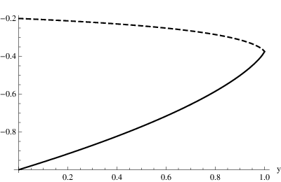
As one can see in Figure 2, the factor −[Ψ⁡(y)+y​Ψ′​(y)]-\left[\,\Psi(y)\,+\,y\,\Psi^{\prime}(y)\,\right] is negative for y∈[0,1]y\in[0,1]. At the same time, from Eq. (243) we know that Ψ′​(y)\Psi^{\prime}(y) is negative for y≥0y\geq 0 (see also the corresponding plot in Figure 2). Thus, for a positive gluon propagator 𝒟⁡(p2)\mathcal{D}(p^{2}), the 3​d3d derivative ∂σ⁡(p2)/∂p2\partial\sigma(p^{2})/\partial p^{2} is negative for p2>0p^{2}>0.

Refer to caption
Figure 2: The functions −[Ψ⁡(y)+y​Ψ′​(y)]-\left[\,\Psi(y)\,+\,y\,\Psi^{\prime}(y)\,\right] (full line) and Ψ′​(y)\Psi^{\prime}(y) (dashed line) for y∈[0,1]y\in[0,1].

Finally, we can consider a general d>2d>2 and, after suitable changes of variables (for p2>0p^{2}>0), we write

1g2​Nc​∂σ⁡(p2)∂p2\displaystyle\frac{1}{g^{2}N_{c}}\,\frac{\partial\sigma(p^{2})}{\partial p^{2}} =\displaystyle= Ωd(2​π)dd−1dpd−42{∫01dyy2−d/2𝒟(p2/y)2F1′(1,1−d/2;1+d/2;y)\displaystyle\frac{\Omega_{d}}{(2\pi)^{d}}\,\frac{d-1}{d}\,\frac{p^{d-4}}{2}\,\left\{\int_{0}^{1}\,\mathrm{d}y\,y^{2-d/2}\;\mathcal{D}(p^{2}/y)\;\;_{2}F^{\prime}_{1}\left(1,1-d/2;1+d/2;y\right)\right. (52)
−∫01dyyd/2−1𝒟(yp2)[2F1(1,1−d/2;1+d/2;y)+y2F1′(1,1−d/2;1+d/2;y)]}.\displaystyle\left.\;\;\;-\,\int_{0}^{1}\,\mathrm{d}y\,y^{d/2-1}\;\mathcal{D}(yp^{2})\,\Bigl[\;_{2}F_{1}\left(1,1-d/2;1+d/2;y\right)\,+\,y\;_{2}F^{\prime}_{1}\left(1,1-d/2;1+d/2;y\right)\,\Bigr]\right\}\;.

Note that the dependence on p2p^{2} is only in the global factor pd−4p^{d-4} and in the argument of the gluon propagator. From Appendix B we know that the derivative F1′2​(1,1−d/2,1+d/2,x){}_{2}F^{\prime}_{1}\left(1,1-d/2;1+d/2;x\right) is negative for x∈[0,1]x\in[0,1] and d>2d>2 and that, under the same hypotheses, the expression in square brackets is positive. Thus, for a positive gluon propagator, both term in the r.h.s. of the above expression are negative and we have proven that, for any dimension d≥2d\geq 2, the Gribov form-factor σ⁡(p2)\sigma(p^{2}) (at one loop) is monotonically decreasing with p2p^{2}, i.e. it gets its maximum value at p2=0p^{2}=0.

III Evaluation of the One-Loop Corrected Ghost Propagator Using (Linear Combinations of) Yukawa-Like Gluon Propagators

In the previous Section we have proven that, at one-loop level and for a sufficiently regular gluon propagator 𝒟⁡(p2)\mathcal{D}(p^{2}), the Gribov ghost form-factor σ⁡(p2)\sigma(p^{2}) is always finite in three and four space-time dimensions while, in d=2d=2, one needs to impose 𝒟⁡(0)=0\mathcal{D}(0)=0 in order to avoid an IR singularity of the type −𝒟⁡(0)​ln⁡(p2)-\mathcal{D}(0)\,\ln(p^{2}). In this Section we present an explicit calculation of σ⁡(p2)\sigma(p^{2}) at one loop for d=2,3d=2,3 and 4 using, for the gluon propagator, results recently presented in Ref. [59, 60] from fits to lattice data of 𝒟⁡(p2)\mathcal{D}(p^{2}) in the SU(2) case. The expressions obtained below for the ghost propagator 𝒢⁡(p2)\mathcal{G}(p^{2}) will be used in a subsequent work [95] to model lattice data of SU(2) ghost propagators.

In this Section, besides recovering the same results reported in Section II, we also find that the ghost propagator 𝒢⁡(p2)\mathcal{G}(p^{2}) admits a one-parameter family of behaviors [21, 34] labelled by the coupling constant g2g^{2}, considered as a free parameter. The no-pole condition σ⁡(0)≤1\sigma(0)\leq 1 implies g2≤gc2g^{2}\leq g^{2}_{c}, where gc2g^{2}_{c} is a “critical” value. Moreover, for g2g^{2} smaller than gc2g^{2}_{c} one has σ⁡(0)<1\sigma(0)<1 and the ghost propagator shows a free-like behavior in the IR limit, in agreement with the so-called massive solution of gluon and ghost DSEs [18, 19, 20, 21, 22, 23, 24, 25]. On the contrary, for g2=gc2g^{2}=g^{2}_{c} one finds σ⁡(0)=1\sigma(0)=1 and the ghost propagator is IR enhanced [1, 13, 14, 15, 16].

III.1 Yukawa-Like Gluon Propagators and Set Up

In Ref. [59, 60] the SU(2) gluon propagator was fitted in 2, 3 and 4 space-time dimensions using, respectively, the functions2222 22 Note that, for consistency with the notation used in Ref. [59], in this Section the non-integer power of the momentum pp is η\eta and not 2​η2\eta as in the rest of the manuscript.

𝒟⁡(p2)=C​p2+l​pη+sp4+u2​p2+t2,\mathcal{D}(p^{2})\,=\,C\,\frac{p^{2}+l\,p^{\eta}+s}{p^{4}+u^{2}\,p^{2}+t^{2}}\;, (53)
𝒟⁡(p2)=C​p4+(s+1)​p2+sp6+(k+u2)​p4+(k​u2+t2)​p2+k​t2\mathcal{D}(p^{2})\,=\,C\,\frac{p^{4}+(s+1)p^{2}+s}{p^{6}+(k+u^{2})p^{4}+(ku^{2}+t^{2})p^{2}+kt^{2}} (54)

and

𝒟⁡(p2)=C​p2+sp4+u2​p2+t2.\mathcal{D}(p^{2})\,=\,C\,\frac{p^{2}+s}{p^{4}+u^{2}\,p^{2}+t^{2}}\;. (55)

The last two propagators are tree-level gluon propagators that arise in the study of the RGZ action [82, 83, 84, 85]. The first one is a simple generalization of the form (55) that fits well the 2​d2d data. Note that these three functions can be written as a linear combination of propagators of the type 1/(p2+ω2)1/(p^{2}+\omega^{2}), where ω2\omega^{2} is in general a complex number. [In the 2​d2d case we need to consider the more general form pη/(p2+ω2)p^{\eta}/(p^{2}+\omega^{2}) with η≥0\eta\geq 0.] Thus, in order to evaluate σ⁡(p2)\sigma(p^{2}) in Eq. (7) using the above gluon propagators 𝒟⁡(p2)\mathcal{D}(p^{2}), we first consider the integral

f⁡(p,ω2)=pμ​pνp2​∫dd​q(2​π)d​1(p−q)2​1q2+ω2​(δμ​ν−qμ​qνq2).f(p,\omega^{2})\,=\,\frac{p_{\mu}p_{\nu}}{p^{2}}\int\frac{\mathrm{d}^{d}q}{(2\pi)^{d}}\frac{1}{(p-q)^{2}}\frac{1}{q^{2}+\omega^{2}}\left(\delta_{\mu\nu}-\frac{q_{\mu}q_{\nu}}{q^{2}}\right)\;. (56)

The evaluation of f⁡(p,ω2)f(p,\omega^{2}) can be done in three and four space-time dimensions by introducing Feynman parameters and applying the usual shift in the momentum qq. The integration then yields

f⁡(p2,ω2)\displaystyle f(p^{2},\omega^{2}) =\displaystyle= 1(4​π)d/2​∫01d​x​[Δd/2−2​Γ​(2−d/2)]\displaystyle\frac{1}{(4\pi)^{d/2}}\int_{0}^{1}\mathrm{d}x\left[\Delta^{d/2-2}\,\Gamma(2-d/2)\right] (57)
−1(4​π)d/2∫01dx∫01−xdy[12Θd/2−2Γ(2−d/2)+x2p2Θd/2−3Γ(3−d/2)]\displaystyle\;-\frac{1}{(4\pi)^{d/2}}\int_{0}^{1}\mathrm{d}x\int_{0}^{1-x}\mathrm{d}y\left[\frac{1}{2}\Theta^{d/2-2}\,\Gamma(2-d/2)\,+\,x^{2}p^{2}\,\Theta^{d/2-3}\,\Gamma(3-d/2)\right]

with

Δ\displaystyle\Delta =−x2​p2+x​p2+(1−x)​ω2,\displaystyle=-x^{2}p^{2}+xp^{2}+(1-x)\omega^{2}\;, Θ\displaystyle\Theta =−x2​p2+x​p2+y​ω2.\displaystyle=-x^{2}p^{2}+xp^{2}+y\omega^{2}\;. (58)

Since the Gamma function has the behavior Γ⁡(x)≈1/x\Gamma(x)\approx 1/x for small xx, it is clear that the first two integrals are UV finite for d<4d<4 while the third one is UV finite for d<6d<6. Below we will calculate the integral (57) for d=d= 3 and 4. We start from the case d=3d=3, where all terms are finite, and then we evaluate the integral for the case d=d= 4, using the MS¯\overline{\mbox{MS}} scheme. On the contrary, as stressed above, in the 2​d2d case one needs to evaluate the more general function

f⁡(p,ω2,η)=pμ​pνp2​∫d2​q(2​π)d​1(p−q)2​qηq2+ω2​(δμ​ν−qμ​qνq2)f(p,\omega^{2},\eta)\,=\,\frac{p_{\mu}p_{\nu}}{p^{2}}\int\frac{\mathrm{d}^{2}q}{(2\pi)^{d}}\frac{1}{(p-q)^{2}}\frac{q^{\eta}}{q^{2}+\omega^{2}}\left(\delta_{\mu\nu}-\frac{q_{\mu}q_{\nu}}{q^{2}}\right) (59)

with η≥0\eta\geq 0. This case will be treated (in a slightly different way) in Section III.4.

Most of the analytic results reported in this Section have been checked using Mathematica and/or Maple.

III.2 Ghost Propagator in the 3dd Case

In the 3​d3d case the residual xx- and yy-integrations in Eq. (57) are straightforward and give

f⁡(p2,ω2)\displaystyle f(p^{2},\omega^{2}) =\displaystyle= [14​π​p​arctan⁡(pω2)]+[−(p2−ω2)​ω232​π​p2​ω2+π​p64​π​ω2−(p2+ω2)232​π​p3​ω2​arctan⁡(pω2)]\displaystyle\left[\,\frac{1}{4\pi p}\arctan\left(\frac{p}{\sqrt{\omega^{2}}}\right)\,\right]\,+\,\left[\,-\frac{(p^{2}-\omega^{2})\sqrt{\omega^{2}}}{32\pi p^{2}\omega^{2}}+\frac{\pi p}{64\pi\omega^{2}}-\frac{(p^{2}+\omega^{2})^{2}}{32\pi p^{3}\omega^{2}}\arctan\left(\frac{p}{\sqrt{\omega^{2}}}\right)\,\right] (60)
+[3​(p2−ω2)​ω232​π​p2​ω2+3​p4−2​p2​ω2+3​(ω2)232​π​p3​ω2​arctan⁡(pω2)−3​π​p64​π​ω2],\displaystyle\quad+\,\left[\,\frac{3\,(p^{2}-\omega^{2})\sqrt{\omega^{2}}}{32\pi p^{2}\omega^{2}}+\frac{3p^{4}-2p^{2}\omega^{2}+3(\omega^{2})^{2}}{32\pi p^{3}\omega^{2}}\arctan\left(\frac{p}{\sqrt{\omega^{2}}}\right)-\frac{3\pi p}{64\pi\omega^{2}}\,\right]\;,

where the three square brackets highlight the contribution from the three terms in Eq. (57). Here we have only made the assumption p2>0p^{2}>0. By simplifying the above result, we find

f⁡(p2,ω2)\displaystyle f(p^{2},\omega^{2}) =\displaystyle= 14​π​p​arctan⁡(pω2)+(p2−ω2)​ω216​π​p2​ω2−π​p32​π​ω2+(p2−ω2)216​π​p3​ω2​arctan⁡(pω2)\displaystyle\frac{1}{4\pi p}\arctan\left(\frac{p}{\sqrt{\omega^{2}}}\right)\,+\,\frac{(p^{2}-\omega^{2})\sqrt{\omega^{2}}}{16\pi p^{2}\omega^{2}}\,-\,\frac{\pi p}{32\pi\omega^{2}}\,+\,\frac{(p^{2}-\omega^{2})^{2}}{16\pi p^{3}\omega^{2}}\arctan\left(\frac{p}{\sqrt{\omega^{2}}}\right) (61)
=\displaystyle= 132​π​p3​ω2​g​(p2,ω2)\displaystyle\frac{1}{32\pi p^{3}\omega^{2}}\,g(p^{2},\omega^{2})

where

g⁡(p2,ω2)=−π​p4+ 2​p3​ω2− 2​p​(ω2)3/2+ 2​(p2+ω2)2​arctan⁡(pω2).g(p^{2},\omega^{2})\,=\,-\pi\,p^{4}\,+\,2\,p^{3}\,\sqrt{\omega^{2}}\,-\,2\,p\,(\omega^{2})^{3/2}\,+\,2\,(p^{2}\,+\,\omega^{2})^{2}\,\arctan\left(\frac{p}{\sqrt{\omega^{2}}}\right)\;. (62)

In order to use the result (61) we need to write the gluon propagator (54) as

𝒟⁡(p2)=αp2+ω12+βp2+ω22+γp2+ω32.\mathcal{D}(p^{2})\,=\,\frac{\alpha}{p^{2}+\omega_{1}^{2}}+\frac{\beta}{p^{2}+\omega_{2}^{2}}+\frac{\gamma}{p^{2}+\omega_{3}^{2}}\;. (63)

Here ω12\omega_{1}^{2}, ω22\omega_{2}^{2} and ω32\omega_{3}^{2} are the three roots of the cubic equation, with respect to the variable p2p^{2}, obtained by setting equal to zero the denominator of Eq. (54). Thus, by combining Eqs. (7), (63) and (56) we can write for the function σ⁡(p2)\sigma(p^{2}) in the 3​d3d case the expression

σ⁡(p2)=g2​Nc​[α​f​(p2,ω12)+β​f​(p2,ω22)+γ​f​(p2,ω32)]\sigma(p^{2})\,=\,g^{2}N_{c}\,\left[\alpha f(p^{2},\omega_{1}^{2})\,+\,\beta f(p^{2},\omega_{2}^{2})\,+\,\gamma f(p^{2},\omega_{3}^{2})\right] (64)

or

σ⁡(p2)=g2​Nc32​π​ω2​p3​[α​g​(p2,ω12)+β​g​(p2,ω22)+γ​g​(p2,ω32)]\sigma(p^{2})\,=\,\frac{g^{2}N_{c}}{32\,\pi\,\omega^{2}\,p^{3}}\,\left[\alpha\,g(p^{2},\omega_{1}^{2})\,+\,\beta\,g(p^{2},\omega_{2}^{2})\,+\,\gamma\,g(p^{2},\omega_{3}^{2})\right] (65)

with g⁡(p2,ω2)g(p^{2},\omega^{2}) given in Eq. (62). In general, the roots ω12\omega_{1}^{2}, ω22\omega_{2}^{2} and ω32\omega_{3}^{2} are all real or there is one real root, for example ω12\omega_{1}^{2}, and two complex-conjugate roots, i.e. (ω22)∗=ω32(\omega_{2}^{2})^{*}=\omega_{3}^{2}, implying also β=γ∗\beta=\gamma^{*}. Since the fits in Ref. [59, 60] support the latter case we write

β=a+i​b,γ=a−i​b\beta\,=\,a+ib\;,\qquad\gamma\,=\,a-ib (66)

and

ω22=v+i​w,ω32=v−i​w.\omega_{2}^{2}\,=\,v+iw\;,\qquad\omega_{3}^{2}\,=\,v-iw\;. (67)

Then, following for example [96], we find for ω22\omega_{2}^{2} the relations

ω22\displaystyle\sqrt{\omega_{2}^{2}} =v+i​w=12​v2+w2+v+i2​v2+w2−v,\displaystyle\,=\,\sqrt{v+iw}\,=\,\frac{1}{\sqrt{2}}\sqrt{\sqrt{v^{2}+w^{2}}+v}+\frac{i}{\sqrt{2}}\sqrt{\sqrt{v^{2}+w^{2}}-v}\;, (68)
(ω22)3/2\displaystyle\left(\omega_{2}^{2}\right)^{3/2} =(v+i​w)3/2=(v+i​w)​v+i​w,\displaystyle\,=\,(v+iw)^{3/2}\,=\,(v+iw)\sqrt{v+iw}\;, (69)
pω22\displaystyle\frac{p}{\sqrt{\omega_{2}^{2}}} =pv+i​w=pv2+w2​v−i​w\displaystyle\,=\,\frac{p}{\sqrt{v+iw}}\,=\,\frac{p}{\sqrt{v^{2}+w^{2}}}\,\sqrt{v-iw} (70)

and similar results for ω32\omega_{3}^{2}. We also use the expression (see for example [97])

arctan⁡(z)=12​arg⁡(i−zi+z)−i2​ln⁡|i−zi+z|∀z≠{i,−i}.\arctan\left(z\right)\,=\,\frac{1}{2}\arg\left(\frac{i-z}{i+z}\right)-\frac{i}{2}\ln\left|\frac{i-z}{i+z}\right|\qquad\forall z\not=\{i,-i\}\;. (71)

This allows us to write the function σ⁡(p2)\sigma(p^{2}) only in term of real quantities, i.e.

σ⁡(p2)=g2​Nc8​[α​g​(p2,ω12)4​π​ω12​p3+fR​(p2)]\sigma(p^{2})\,=\,\frac{g^{2}N_{c}}{8}\left[\frac{\alpha g(p^{2},\omega_{1}^{2})}{4\,\pi\,\omega_{1}^{2}\,p^{3}}\,+\,f_{R}(p^{2})\right] (72)

where g⁡(p2,ω2)g(p^{2},\omega^{2}) is given in Eq. (62) above. Also, we have

fR​(p2)=f1​(p2)+f2​(p2)+f3​(p2)+f4​(p2)+f5​(p2)f_{R}(p^{2})\,=\,f_{1}(p^{2})\,+\,f_{2}(p^{2})\,+\,f_{3}(p^{2})\,+\,f_{4}(p^{2})\,+\,f_{5}(p^{2}) (73)

with

f1​(p2)\displaystyle f_{1}(p^{2}) =\displaystyle= −p​a​v+b​w2​R2,\displaystyle-p\;\frac{av\,+\,bw}{2\,R^{2}}\;, (74)
f2​(p2)\displaystyle f_{2}(p^{2}) =\displaystyle= (a​v+b​w)​R+v−(b​v−a​w)​R−v2​π​R2,\displaystyle\frac{\left(av\,+\,bw\right)\sqrt{R+v}\,-\,\left(bv\,-\,aw\right)\sqrt{R-v}}{\sqrt{2}\,\pi\,R^{2}}\;, (75)
f3​(p2)\displaystyle f_{3}(p^{2}) =\displaystyle= −1p2​a​R+v−b​R−v2​π,\displaystyle-\frac{1}{p^{2}}\,\frac{a\sqrt{R+v}\,-\,b\sqrt{R-v}}{\sqrt{2}\,\pi}\;, (76)
f4​(p2)\displaystyle f_{4}(p^{2}) =\displaystyle= A⁡(p2)​p4​(a​v+b​w)+ 2​a​p2​R2+R2​(a​v−b​w)2​π​R2​p3,\displaystyle A(p^{2})\;\frac{p^{4}\left(av\,+\,bw\right)\,+\,2\,a\,p^{2}\,R^{2}\,+\,R^{2}\left(av\,-\,bw\right)}{2\,\pi\,R^{2}\,p^{3}}\;, (77)
f5​(p2)\displaystyle f_{5}(p^{2}) =\displaystyle= −L⁡(p2)​p4​(b​v−a​w)+ 2​b​p2​R2+R2​(b​v+a​w)2​π​R2​p3\displaystyle-L(p^{2})\;\frac{p^{4}\left(bv\,-\,aw\right)\,+\,2\,b\,p^{2}\,R^{2}\,+\,R^{2}\left(bv\,+\,aw\right)}{2\,\pi\,R^{2}\,p^{3}} (78)

and

A⁡(p2)\displaystyle A(p^{2}) =\displaystyle= {arctan⁡(2​p​R+vR−p2)if​R−p2>0π+arctan⁡(2​p​R+vR−p2)if​R−p2<0,\displaystyle\left\{\begin{array}[]{ll}\arctan\left(\frac{\sqrt{2}\,p\,\sqrt{R+v}}{R\,-\,p^{2}}\right)&\mbox{if}\;\;\;R\,-\,p^{2}>0\\[8.53581pt] \pi\,+\,\arctan\left(\frac{\sqrt{2}\,p\,\sqrt{R+v}}{R\,-\,p^{2}}\right)&\mbox{if}\;\;\;R\,-\,p^{2}<0\end{array}\right.\;,
L⁡(p2)\displaystyle L(p^{2}) =\displaystyle= ln⁡[p4+ 2​p2​v+R2R+p⁡(p+2​R−v)],\displaystyle\ln\left[\frac{\sqrt{p^{4}\,+\,2\,p^{2}\,v\,+\,R^{2}}}{R\,+\,p\,\left(p\,+\,\sqrt{2}\,\sqrt{R-v}\right)}\right]\;, (82)
R\displaystyle R =\displaystyle= v2+w2.\displaystyle\sqrt{v^{2}+w^{2}}\;. (83)

One can check that σ⁡(p2)\sigma(p^{2}) is null in the limit p→∞p\to\infty. Finally, by expanding σ⁡(p2)\sigma(p^{2}) around p2=0p^{2}=0 in Eqs. (72)–(83) we find

σ⁡(p2)g2​Nc\displaystyle\frac{\sigma(p^{2})}{g^{2}N_{c}} =\displaystyle= α6​π​ω12+R+v​9​a​R2−(a​v−b​w)​(2​v−R)24​2​π​R3\displaystyle\frac{\alpha}{6\pi\sqrt{\omega_{1}^{2}}}\,+\,\sqrt{R+v}\;\frac{9\,a\,R^{2}-\left(a\,v-b\,w\right)\,\left(2\,v-R\right)}{24\,\sqrt{2}\,\pi\,R^{3}} (84)
+R−v​9​b​R2−(b​v+a​w)​(2​v+R)24​2​π​R3−α​R2+2​(a​v+b​w)​ω1232​ω12​R2​p+O⁡(p2),\displaystyle\quad+\sqrt{R-v}\;\frac{9\,b\,R^{2}-\left(b\,v+a\,w\right)\,\left(2\,v+R\right)}{24\,\sqrt{2}\,\pi\,R^{3}}\,-\,\frac{\alpha\,R^{2}+2\,(a\,v+b\,w)\omega_{1}^{2}}{32\,\omega_{1}^{2}\,R^{2}}\,p\,+\,O\left(p^{2}\right)\;,

which implies 𝒢⁡(p2)∝p−2\mathcal{G}(p^{2})\propto p^{-2} at very small momenta. However, if the constant term in the above expression is equal to 1/(g2​Nc)1/(g^{2}N_{c}), yielding σ⁡(0)=1\sigma(0)=1, then one gets in the IR limit 𝒢⁡(p2)∝p−4\mathcal{G}(p^{2})\propto p^{-4} or 𝒢⁡(p2)∝p−3\mathcal{G}(p^{2})\propto p^{-3}, depending on whether the term α​R2+2​(a​v+b​w)​ω12\alpha\,R^{2}+2\,(a\,v+b\,w)\omega_{1}^{2} vanishes or not. In particular, in the original GZ case, i.e. when the terms containing ω12\omega_{1}^{2} and α\alpha are absent, we do recover the usual 1/p41/p^{4} behavior. Also note that for purely imaginary poles, i.e. when v=b=0v=b=0 (and R=wR=w), the condition σ⁡(0)=1\sigma(0)=1 simplifies to

αω12+2​aw=6​πg2​Nc.\frac{\alpha}{\sqrt{\omega_{1}^{2}}}\,+\,\frac{\sqrt{2}\,a}{\sqrt{w}}\,=\,\frac{6\pi}{g^{2}N_{c}}\;. (85)

Clearly, for a given value of NcN_{c} and with a suitable choice of g2g^{2}, one can always set σ⁡(0)=1\sigma(0)=1 in Eq. (84). For example, using the numerical data in the second column of Table XI of Ref. [59] and Nc=2N_{c}=2, we find from Eq. (84) the result2323 23 The errors in brackets have been evaluated using a Monte Carlo analysis with 10000 samples (see Ref. [59] for details).

σ⁡(p2)2​g2≈ 0.039​(0.001)−0.017​(0.003)​p+O⁡(p2)\frac{\sigma(p^{2})}{2\,g^{2}}\,\approx\,0.039(0.001)-0.017(0.003)\,p\,+\,O\left(p^{2}\right) (86)

and we have σ⁡(0)=1\sigma(0)=1 if g2≈12.82g^{2}\approx 12.82. Thus, if one considers g2g^{2} as a free parameter, then Eq. (84) gives a one-parameter family of behaviors, labeled by g2g^{2}. For a specific value of g2=gc2g^{2}=g^{2}_{c} we have σ⁡(0)=1\sigma(0)=1 and one finds an IR-enhanced ghost propagator at one loop. On the contrary, for g2<gc2g^{2}<g^{2}_{c} we obtain σ⁡(0)<1\sigma(0)<1 and 𝒢⁡(p2)∝p−2\mathcal{G}(p^{2})\propto p^{-2} in the IR limit. Finally, for g2>gc2g^{2}>g^{2}_{c} the no-pole condition σ⁡(0)≤1\sigma(0)\leq 1 is not satisfied, i.e. the ghost propagator is negative in the IR limit. These findings are in qualitative agreement with the DSE results obtained in Refs. [21, 34]. Finally, note that at small momenta the function σ⁡(p2)\sigma(p^{2}) in the above formula (86) is decreasing as p2p^{2} increases, as expected from Section II.4.

III.3 Ghost Propagator in the 4dd Case

We want now to evaluate f⁡(p2,ω2)f(p^{2},\omega^{2}) in Eq. (57) for d=4d=4. As stressed above, in this case we have to deal with UV divergences. We do the calculation in the MS¯\overline{\mbox{MS}} renormalization scheme using dimensional regularization with d=4−εd=4-\varepsilon. For the first term in Eq. (57) we have

(4​π)2−d/216​π2​∫01d​x​[Δd/2−2​Γ​(2−d/2)]=116​π2​∫01d​x​[2ε−γE+ln⁡(4​π)−ln⁡(Δ)],\frac{(4\pi)^{2-d/2}}{16\pi^{2}}\int_{0}^{1}\mathrm{d}x\left[\Delta^{d/2-2}\,\Gamma(2-d/2)\right]\,=\,\frac{1}{16\pi^{2}}\int_{0}^{1}\mathrm{d}x\left[\frac{2}{\varepsilon}\,-\,\gamma_{E}\,+\,\ln\left(4\pi\right)\,-\,\ln\left(\Delta\right)\right]\;, (87)

where γE\gamma_{E} is the Euler constant. Then, using the usual MS¯\overline{\mbox{MS}} prescription, we find

−116​π2​∫01d​x​ln⁡[−x2​p2+x​p2+(1−x)​ω2μ¯2]=−116​π2​∫01d​x​[ln⁡(p2μ¯2)+ln⁡(1−x)+ln⁡(x+ω2p2)]\frac{-1}{16\pi^{2}}\int_{0}^{1}\mathrm{d}x\,\ln\left[\frac{-x^{2}p^{2}+xp^{2}+(1-x)\omega^{2}}{\overline{\mu}^{2}}\right]\,=\,\frac{-1}{16\pi^{2}}\int_{0}^{1}\mathrm{d}x\left[\ln\left(\frac{p^{2}}{\overline{\mu}^{2}}\right)\,+\,\ln\left(1-x\right)\,+\,\ln\left(x+\frac{\omega^{2}}{p^{2}}\right)\right] (88)

and the d​x\mathrm{d}x integration yields

−116​π2​[ln⁡(p2μ¯2)− 2−ω2p2​ln⁡(ω2p2)+(1+ω2p2)​ln⁡(1+ω2p2)]\displaystyle\frac{-1}{16\pi^{2}}\left[\ln\left(\frac{p^{2}}{\overline{\mu}^{2}}\right)\,-\,2\,-\,\frac{\omega^{2}}{p^{2}}\ln\left(\frac{\omega^{2}}{p^{2}}\right)\,+\,\left(1+\frac{\omega^{2}}{p^{2}}\right)\ln\left(1+\frac{\omega^{2}}{p^{2}}\right)\right] (89)
=\displaystyle= −116​p2​π2​[−2​p2+p2​ln⁡(p2+ω2μ¯2)+ω2​ln⁡(p2+ω2ω2)],\displaystyle\frac{-1}{16\,p^{2}\pi^{2}}\left[-2p^{2}\,+\,p^{2}\,\ln\left(\frac{p^{2}+\omega^{2}}{\overline{\mu}^{2}}\right)\,+\,\omega^{2}\,\ln\left(\frac{p^{2}+\omega^{2}}{\omega^{2}}\right)\right]\;,

where μ¯\overline{\mu} is the renormalization scale. For the second term in Eq. (57), which is also divergent, we first perform the yy integration exactly, obtaining

−Γ⁡(2−d/2)(4​π)d/2​ω2​(d−2)∫01dx(−x2p2+xp2)d/2−1[(1+ω2x​p2)d/2−1− 1].-\frac{\Gamma(2-d/2)}{(4\pi)^{d/2}\,\omega^{2}\,\left(d-2\right)}\int_{0}^{1}\mathrm{d}x\,\left(-x^{2}p^{2}+xp^{2}\right)^{d/2-1}\,\left[\left(1+\frac{\omega^{2}}{xp^{2}}\right)^{d/2-1}\,-\,1\right]\;. (90)

The ε\varepsilon expansion then gives

132​π2​∫01d​x​(1−x)​[ln⁡(−x2​p2+x​p2μ¯2)+(1+x​p2ω2)​ln⁡(1+ω2x​p2)−1],\frac{1}{32\pi^{2}}\int_{0}^{1}\mathrm{d}x\,\left(1-x\right)\,\left[\ln\left(\frac{-x^{2}p^{2}+xp^{2}}{\overline{\mu}^{2}}\right)\,+\,\left(1+\frac{xp^{2}}{\omega^{2}}\right)\ln\left(1+\frac{\omega^{2}}{xp^{2}}\right)\,-1\,\right]\;, (91)

where we have already applied the MS¯\overline{\mbox{MS}} prescription, and after integrating in d​x\mathrm{d}x we find

1192​p4​ω2​π2​{p4​(p2+3​ω2)​ln⁡(ω2p2)+(p2+ω2)3​ln⁡(p2+ω2ω2)+p2​ω2​[−7​p2−ω2+3​p2​ln⁡(p2μ¯2)]}.\frac{1}{192p^{4}\omega^{2}\pi^{2}}\,\left\{p^{4}\left(p^{2}+3\omega^{2}\right)\ln\left(\frac{\omega^{2}}{p^{2}}\right)\,+\,\left(p^{2}+\omega^{2}\right)^{3}\ln\left(\frac{p^{2}+\omega^{2}}{\omega^{2}}\right)\,+\,p^{2}\omega^{2}\left[-7p^{2}-\omega^{2}+3p^{2}\ln\left(\frac{p^{2}}{\overline{\mu}^{2}}\right)\right]\right\}\;. (92)

Finally, the third term, which is finite, yields

−116​π2∫01dx∫01−xdy[x2p2Θ−1]=−116​π2​ω2∫01dxx2p2[ln(x+ω2p2)−ln(x)]\displaystyle-\frac{1}{16\pi^{2}}\int_{0}^{1}\mathrm{d}x\int_{0}^{1-x}\mathrm{d}y\left[x^{2}p^{2}\,\Theta^{-1}\right]\,=\,-\frac{1}{16\pi^{2}\omega^{2}}\int_{0}^{1}\mathrm{d}x\,x^{2}p^{2}\,\left[\ln\left(x+\frac{\omega^{2}}{p^{2}}\right)\,-\,\ln\left(x\right)\right] (93)
=\displaystyle= −196​p4​ω2​π2​[p2​ω2​(p2−2​ω2)+ 2​p6​ln⁡(ω2p2)+ 2​(p6+ω6)​ln⁡(p2+ω2ω2)].\displaystyle-\frac{1}{96p^{4}\omega^{2}\pi^{2}}\,\left[\,p^{2}\omega^{2}(p^{2}-2\omega^{2})\,+\,2\,p^{6}\ln\left(\frac{\omega^{2}}{p^{2}}\right)\,+\,2\left(p^{6}+\omega^{6}\right)\ln\left(\frac{p^{2}+\omega^{2}}{\omega^{2}}\right)\,\right]\;. (94)

By summing the three results above we ultimately find (in the MS¯\overline{\mbox{MS}} scheme)

f⁡(p2,ω2)=164​p4​ω2​π2​[f1​(p2,ω)+f2​(p2,ω2)+f3​(p2,ω2)]f(p^{2},\omega^{2})\,=\,\frac{1}{64p^{4}\omega^{2}\pi^{2}}\,\left[\,f_{1}(p^{2},\omega)\,+\,f_{2}(p^{2},\omega^{2})\,+\,f_{3}(p^{2},\omega^{2})\,\right] (95)

with

f1​(p2,ω)\displaystyle f_{1}(p^{2},\omega) =\displaystyle= p4​(ω2−p2)​ln⁡(ω2p2),\displaystyle p^{4}\left(\omega^{2}-p^{2}\right)\ln\left(\frac{\omega^{2}}{p^{2}}\right)\;, (96)
f2​(p2,ω)\displaystyle f_{2}(p^{2},\omega) =\displaystyle= −(p6−p4​ω2+3​p2​ω4+ω6)​ln⁡(p2+ω2ω2),\displaystyle-\,\left(p^{6}-p^{4}\omega^{2}+3\,p^{2}\omega^{4}+\omega^{6}\right)\ln\left(\frac{p^{2}+\omega^{2}}{\omega^{2}}\right)\;, (97)
f3​(p2,ω)\displaystyle f_{3}(p^{2},\omega) =\displaystyle= p2​ω2​[5​p2+ω2+p2​ln⁡(p2μ¯2)−4​p2​ln⁡(p2+ω2μ¯2)].\displaystyle p^{2}\omega^{2}\left[5\,p^{2}+\omega^{2}+p^{2}\,\ln\left(\frac{p^{2}}{\overline{\mu}^{2}}\right)-4\,p^{2}\,\ln\left(\frac{p^{2}+\omega^{2}}{\overline{\mu}^{2}}\right)\right]\;. (98)

As shown in Ref. [59, 60], in the 4​d4d case the fit of the gluon-propagator data is done using the expression (55). Thus, in order to use the above result (95)–(98), we need to write the gluon propagator as

𝒟⁡(p2)=α+p2+ω+2+α−p2+ω−2,\mathcal{D}(p^{2})\,=\,\frac{\alpha_{+}}{p^{2}+\omega_{+}^{2}}+\frac{\alpha_{-}}{p^{2}+\omega_{-}^{2}}\;, (99)

where ω±\omega_{\pm} are the roots of the quadratic equation, with respect to the variable p2p^{2}, obtained by setting equal to zero the denominator of Eq. (55). Then, the ghost form-factor in the MS¯\overline{\mbox{MS}} scheme is given by

σMS¯​(p2)=g2​Nc​[α+​f​(p2,ω+2)+α−​f​(p2,ω−2)]\sigma^{\overline{\mbox{\tiny{MS}}}}(p^{2})\,=\,g^{2}N_{c}\,\left[\,\alpha_{+}\,f(p^{2},\omega_{+}^{2})\,+\,\alpha_{-}\,f(p^{2},\omega_{-}^{2})\,\right] (100)

and we have

𝒢MS¯​(p2)=1p2​[ 1−σMS¯​(p2)]−1.\mathcal{G}^{\overline{\mbox{\tiny{MS}}}}(p^{2})\,=\,\frac{1}{p^{2}}\,\left[\,1\,-\,\sigma^{\overline{\mbox{\tiny{MS}}}}(p^{2})\,\right]^{-1}\;. (101)

Note that the function σMS¯​(p2)\sigma^{\overline{\mbox{\tiny{MS}}}}(p^{2}) is real. From [59, 60] we know that ω±2\omega_{\pm}^{2} are complex-conjugate roots, i.e. ω−2=(ω+2)∗\omega_{-}^{2}=(\omega_{+}^{2})^{*} and α−=α+∗\alpha_{-}=\alpha_{+}^{*}. By writing α±=a±i​b\alpha_{\pm}=a\pm ib and ω±2=v±i​w\omega_{\pm}^{2}=v\pm iw we find

σMS¯​(p2)=g2​Nc32​π2​R2​[−p2​t1​(p2)+R2​t2​(p2)+p−2​t3​(p2)−p−4​t4​(p2)]\sigma^{\overline{\mbox{\tiny{MS}}}}(p^{2})\,=\,\frac{g^{2}N_{c}}{32\pi^{2}R^{2}}\left[-p^{2}t_{1}(p^{2})\,+\,R^{2}t_{2}(p^{2})\,+\,p^{-2}t_{3}(p^{2})\,-\,p^{-4}t_{4}(p^{2})\right] (102)

with

t1​(p2)\displaystyle t_{1}(p^{2}) =\displaystyle= (a​v+b​w)​[ℓ2​(p2)+ℓ3​(p2)]−(b​v−a​w)​[a1​(p2)−a2​(p2)],\displaystyle(av+bw)[\ell_{2}(p^{2})+\ell_{3}(p^{2})]\,-\,(bv-aw)[a_{1}(p^{2})-a_{2}(p^{2})]\;, (103)
t2​(p2)\displaystyle t_{2}(p^{2}) =\displaystyle= a⁡[5+ℓ1​(p2)+ℓ2​(p2)+ℓ3​(p2)−4​ℓ4​(p2)]−b⁡[a1​(p2)−a2​(p2)−4​a3​(p2)],\displaystyle a[5+\ell_{1}(p^{2})+\ell_{2}(p^{2})+\ell_{3}(p^{2})-4\ell_{4}(p^{2})]\,-\,b[a_{1}(p^{2})-a_{2}(p^{2})-4a_{3}(p^{2})]\;, (104)
t3​(p2)\displaystyle t_{3}(p^{2}) =\displaystyle= [1−3​ℓ3​(p2)]​(a​v3−b​w​v2+v​a​w2−b​w3)− 3​a2​(p2)​(b​v3+a​w​v2+v​b​w2+a​w3),\displaystyle[1-3\ell_{3}(p^{2})](av^{3}-bwv^{2}+vaw^{2}-bw^{3})\,-\,3a_{2}(p^{2})(bv^{3}+awv^{2}+vbw^{2}+aw^{3})\;, (105)
t4​(p2)\displaystyle t_{4}(p^{2}) =\displaystyle= ℓ3​(p2)​(a​v4−2​w​b​v3−2​v​b​w3−a​w4)+a2​(p2)​(b​v4+2​a​w​v3+2​v​a​w3−b​w4)\displaystyle\ell_{3}(p^{2})(av^{4}-2wbv^{3}-2vbw^{3}-aw^{4})\,+\,a_{2}(p^{2})(bv^{4}+2awv^{3}+2vaw^{3}-bw^{4}) (106)

and

ℓ1​(p2)\displaystyle\ell_{1}(p^{2}) =\displaystyle= ln⁡(p2μ¯2),\displaystyle\ln\left(\frac{p^{2}}{\overline{\mu}^{2}}\right)\;, (107)
ℓ2​(p2)\displaystyle\ell_{2}(p^{2}) =\displaystyle= ln⁡(Rp2),\displaystyle\ln\left(\frac{R}{p^{2}}\right)\;, (108)
ℓ3​(p2)\displaystyle\ell_{3}(p^{2}) =\displaystyle= ln⁡(R2​p4+R4+2​v​R2​p2R2),\displaystyle\ln\left(\frac{\sqrt{R^{2}p^{4}+R^{4}+2vR^{2}p^{2}}}{R^{2}}\right)\;, (109)
ℓ4​(p2)\displaystyle\ell_{4}(p^{2}) =\displaystyle= ln⁡(p4+2​v​p2+R2μ¯2),\displaystyle\ln\left(\frac{\sqrt{p^{4}+2vp^{2}+R^{2}}}{\overline{\mu}^{2}}\right)\;, (110)
a1​(p2)\displaystyle a_{1}(p^{2}) =\displaystyle= arctan⁡(wv),\displaystyle\arctan\left(\frac{w}{v}\right)\;, (111)
a2​(p2)\displaystyle a_{2}(p^{2}) =\displaystyle= arctan⁡(w​p2R2+v​p2),\displaystyle\arctan\left(\frac{wp^{2}}{R^{2}+vp^{2}}\right)\;, (112)
a3​(p2)\displaystyle a_{3}(p^{2}) =\displaystyle= arctan⁡(wv+p2),\displaystyle\arctan\left(\frac{w}{v+p^{2}}\right)\;, (113)
R\displaystyle R =\displaystyle= v2+w2.\displaystyle\sqrt{v^{2}+w^{2}}\;. (114)

Also note that, at large momenta, one gets

σMS¯​(p2)≈−3​a​g2​Nc32​π2​ln⁡(p2μ¯2).\sigma^{\overline{\mbox{\tiny{MS}}}}(p^{2})\approx-\frac{3\,a\,g^{2}\,N_{c}}{32\,\pi^{2}}\,\ln\left(\frac{p^{2}}{\overline{\mu}^{2}}\right)\;. (115)

Finally, by expanding σMS¯​(p2)\sigma^{\overline{\mbox{\tiny{MS}}}}(p^{2}) around p2=0p^{2}=0 in Eqs. (102)–(114) we obtain

σMS¯​(p2)g2​Nc\displaystyle\frac{\sigma^{\overline{\mbox{\tiny{MS}}}}(p^{2})}{g^{2}N_{c}} =\displaystyle= −6​a​ln⁡(Rμ¯2)−6​b​arctan⁡(wv)−5​a64​π2\displaystyle-\frac{6\,a\,\ln\left(\frac{R}{\overline{\mu}^{2}}\right)-6\,b\,\arctan\left(\frac{w}{v}\right)-5\,a}{64\,\pi^{2}} (116)
+[−11+6​ln⁡(p2R)]​(a​v+w​b)+6​(b​v−a​w)​arctan⁡(wv)192​π2​R2​p2+O⁡(p4).\displaystyle\quad+\frac{\left[-11+6\ln\left(\frac{p^{2}}{R}\right)\right]\,\left(a\,v+w\,b\right)+6(b\,v-a\,w)\,\arctan\left({\frac{w}{v}}\right)}{192\,\pi^{2}\,R^{2}}\,p^{2}\,+\,O\left({p}^{4}\right)\;.

Thus, if σMS¯​(0)=1\sigma^{\overline{\mbox{\tiny{MS}}}}(0)=1 we have that 𝒢MS¯​(p2)∼1/p4\mathcal{G}^{\overline{\mbox{\tiny{MS}}}}(p^{2})\sim 1/p^{4} at small momenta (plus logarithmic corrections). Clearly, also in 4​d4d, we obtain a one-parameter family of behaviors, labelled by the value of g2g^{2}, and the IR-enhanced ghost propagator corresponds to the upper value of g2g^{2} allowed by the no-pole condition (3). With the numerical values reported in the second column of Table IV of Ref. [59] and Nc=2N_{c}=2 we find2424 24 Again, the error in parentheses have been evaluated using a Monte Carlo analysis with 10000 samples.

σMS¯​(p2)2​g2= 0.0240​(0.0007)+[−0.0082​(0.0003)+ 0.0060​(0.0002)​ln⁡(p2)]​p2\frac{\sigma^{\overline{\mbox{\tiny{MS}}}}(p^{2})}{2\,g^{2}}\,=\,0.0240(0.0007)\,+\,\left[-0.0082(0.0003)\,+\,0.0060(0.0002)\ln\left(p^{2}\right)\right]\,p^{2} (117)

and the condition σMS¯​(0)=1\sigma^{\overline{\mbox{\tiny{MS}}}}(0)=1 corresponds2525 25 Clearly, different renormalization schemes will modify the constant term in Eq. (117) and the value of gc2g^{2}_{c}. to gc2≈20.83g^{2}_{c}\approx 20.83. Note again the negative sign of the leading order corrections at small momenta (see Section II.4).

III.4 Ghost Propagator in the 2dd Case

As stressed in Section III.1 above, Ref. [59] has shown that the fit of the gluon-propagator data in the 2​d2d case can be done using the expression

𝒟⁡(p2)=α++i​c​pηp2+ω+2+α−−i​c​pηp2+ω−2,\mathcal{D}(p^{2})\,=\,\frac{\alpha_{+}\,+\,icp^{\eta}}{p^{2}+\omega_{+}^{2}}\,+\,\frac{\alpha_{-}\,-\,icp^{\eta}}{p^{2}+\omega_{-}^{2}}\;, (118)

where cc is real, α−=α+∗\alpha_{-}=\alpha_{+}^{*}, ω−2=(ω+2)∗\omega_{-}^{2}=(\omega_{+}^{2})^{*} and ω±\omega_{\pm} are the roots of the quadratic equation, with respect to the variable p2p^{2}, obtained by setting equal to zero the denominator of Eq. (53). Thus, in order to evaluate the ghost form-factor σ⁡(p2)\sigma(p^{2}) we need to consider the function f⁡(p,ω2,η)f(p,\omega^{2},\eta), defined in Eq. (59) above. To this end, we can choose again the positive xx direction parallel to the external momentum pp and consider polar coordinates. Then, after evaluating the angular integral we find

f⁡(p,ω2,η)=14​π​[∫0pd​qp2​q1+ηq2+ω2+∫p∞d​qq1−η​1q2+ω2],f(p,\omega^{2},\eta)\,=\,\frac{1}{4\pi}\left[\,\int_{0}^{p}\frac{\mathrm{d}q}{p^{2}}\,\frac{q^{1+\eta}}{q^{2}+\omega^{2}}\,+\,\int_{p}^{\infty}\frac{\mathrm{d}q}{q^{1-\eta}}\,\frac{1}{q^{2}+\omega^{2}}\,\right]\;, (119)

valid both for η=0\eta=0 and for η>0\eta>0.

In the case η=0\eta=0 the momentum integration is straightforward giving

f⁡(p,ω2)\displaystyle f(p,\omega^{2}) =\displaystyle= limΛ→∞14​π​[∫0pd​qp2​qq2+ω2+∫pΛd​qq​1q2+ω2]\displaystyle\lim_{\Lambda\to\infty}\,\frac{1}{4\pi}\left[\,\int_{0}^{p}\frac{\mathrm{d}q}{p^{2}}\,\frac{q}{q^{2}+\omega^{2}}\,+\,\int_{p}^{\Lambda}\frac{\mathrm{d}q}{q}\,\frac{1}{q^{2}+\omega^{2}}\,\right] (120)
=\displaystyle= limΛ→∞14​π​{12​p2​ln⁡(1+p2ω2)+1ω2​[ln⁡(Λ)−ln⁡(p)−12​ln⁡(Λ2+ω2)+12​ln⁡(p2+ω2)]}\displaystyle\lim_{\Lambda\to\infty}\,\frac{1}{4\pi}\left\{\,\frac{1}{2p^{2}}\,\ln\left(1+\frac{p^{2}}{\omega^{2}}\right)\,+\,\frac{1}{\omega^{2}}\,\left[\ln\left(\Lambda\right)\,-\,\ln\left(p\right)\,-\,\frac{1}{2}\ln\left(\Lambda^{2}+\omega^{2}\right)\,+\,\frac{1}{2}\ln\left(p^{2}+\omega^{2}\right)\right]\,\right\} (121)
=\displaystyle= 18​π​[1p2​ln⁡(1+p2ω2)+1ω2​ln⁡(1+ω2p2)].\displaystyle\frac{1}{8\pi}\left[\,\frac{1}{p^{2}}\,\ln\left(1+\frac{p^{2}}{\omega^{2}}\right)\,+\,\frac{1}{\omega^{2}}\,\ln\left(1+\frac{\omega^{2}}{p^{2}}\right)\,\right]\;. (122)

Note that the second term above blows up logarithmically in the IR limit p→0p\to 0, in agreement with the result obtained in Section II.2.

For η>0\eta>0 the second integral in Eq. (119) can be written, after the change of variable t=ω2/(q2+ω2)t=\omega^{2}/(q^{2}+\omega^{2}), as

∫p∞d​qq1−η​1q2+ω2=12​(ω2)1−η/2​B​(ω2p2+ω2,1−η2,η2),\int_{p}^{\infty}\frac{\mathrm{d}q}{q^{1-\eta}}\,\frac{1}{q^{2}+\omega^{2}}\,=\,\frac{1}{2(\omega^{2})^{1-\eta/2}}\,B\left(\frac{\omega^{2}}{p^{2}+\omega^{2}};1-\frac{\eta}{2},\frac{\eta}{2}\right)\;, (123)

where

B⁡(x,a,b)=∫0xd​t​ta−1​(1−t)b−1B\left(x;a,b\right)\,=\,\int_{0}^{x}\,\mathrm{d}t\,t^{a-1}\,\left(1-t\right)^{b-1} (124)

is the incomplete Beta function, which is defined for a,b>0a,b>0 [97], implying 2>η>02>\eta>0 in our case. For the first integral in Eq. (119) we cannot use directly the changes of variable v=1/qv=1/q and t=1/(1+ω2​v2)t=1/(1+\omega^{2}v^{2}) because we get an incomplete Beta function (124) with b<0b<0. In this case it is convenient to introduce a Feynman parameter (using non-integer exponents) and write

∫0pd​qp2​q3q2−η​1q2+ω2\displaystyle\int_{0}^{p}\frac{\mathrm{d}q}{p^{2}}\,\frac{q^{3}}{q^{2-\eta}}\,\frac{1}{q^{2}+\omega^{2}} =\displaystyle= 1p2(1−η2)∫01dxx−η/2∫0pq3​d​q[q2+(1−x)​ω2]2−η/2\displaystyle\frac{1}{p^{2}}\left(1-\frac{\eta}{2}\right)\int_{0}^{1}\mathrm{d}x\,x^{-\eta/2}\,\int_{0}^{p}\frac{q^{3}\,\mathrm{d}q}{\left[q^{2}+(1-x)\omega^{2}\right]^{2-\eta/2}} (126)
=\displaystyle= 12​p2∫01dxx−η/2{−p2[p2+(1−x)​ω2]1−η/2\displaystyle\frac{1}{2p^{2}}\int_{0}^{1}\mathrm{d}x\,x^{-\eta/2}\,\Biggl\{\,-\frac{p^{2}}{\left[p^{2}+(1-x)\omega^{2}\right]^{1-\eta/2}}
+2η[p2+(1−x)ω2]η/2−2η[(1−x)ω2]η/2},\displaystyle\qquad\qquad+\,\frac{2}{\eta}\left[p^{2}+(1-x)\omega^{2}\right]^{\eta/2}\,-\,\frac{2}{\eta}\left[(1-x)\omega^{2}\right]^{\eta/2}\,\Biggr\}\;,

where we have also done the integration in d​q\mathrm{d}q. After suitable changes of variables, the last formula can be written as

∫0pd​qp2​q3q2−η​1q2+ω2\displaystyle\!\!\!\!\!\!\!\!\!\int_{0}^{p}\frac{\mathrm{d}q}{p^{2}}\,\frac{q^{3}}{q^{2-\eta}}\,\frac{1}{q^{2}+\omega^{2}} =\displaystyle= −12​(ω2)1−η/2​B​(ω2p2+ω2,1−η2,η2)\displaystyle-\,\frac{1}{2(\omega^{2})^{1-\eta/2}}\,B\left(\frac{\omega^{2}}{p^{2}+\omega^{2}};1-\frac{\eta}{2},\frac{\eta}{2}\right) (127)
+p2+ω2η​p2​(ω2)1−η/2​B​(ω2p2+ω2,1−η2,1+η2)−1ηp2(ω2)−η/2​B​(1−η2,1+η2),\displaystyle\quad\,+\,\frac{p^{2}+\omega^{2}}{\eta\,p^{2}\,(\omega^{2})^{1-\eta/2}}\,B\left(\frac{\omega^{2}}{p^{2}+\omega^{2}};1-\frac{\eta}{2},1+\frac{\eta}{2}\right)\,-\,\frac{1}{\eta\,p^{2}\,(\omega^{2})^{-\eta/2}}\,B\left(1-\frac{\eta}{2},1+\frac{\eta}{2}\right)\;,

where B⁡(a,b)=B⁡(1,a,b)=Γ⁡(a)​Γ​(b)/Γ⁡(a+b)B\left(a,b\right)=B\left(1;a,b\right)=\Gamma(a)\,\Gamma(b)/\Gamma(a+b) is the Beta function. Thus, by summing the two results above, we find

f⁡(p,ω2,η)\displaystyle f(p,\omega^{2},\eta) =\displaystyle= (ω2)η/24​π​η​p2​[p2+ω2ω2​B​(ω2p2+ω2,1−η2,1+η2)−B⁡(1−η2,1+η2)]\displaystyle\frac{(\omega^{2})^{\eta/2}}{4\pi\,\eta\,p^{2}}\,\left[\frac{p^{2}+\omega^{2}}{\omega^{2}}\,B\left(\frac{\omega^{2}}{p^{2}+\omega^{2}};1-\frac{\eta}{2},1+\frac{\eta}{2}\right)\,-\,B\left(1-\frac{\eta}{2},1+\frac{\eta}{2}\right)\right] (128)
=\displaystyle= (ω2)η/2−14​π​η​B​(1−η2,1+η2)\displaystyle\frac{(\omega^{2})^{\eta/2-1}}{4\pi\,\eta}\,B\left(1-\frac{\eta}{2},1+\frac{\eta}{2}\right)
+(ω2)η/24​π​η​p2​p2+ω2ω2​[B⁡(ω2p2+ω2,1−η2,1+η2)−B⁡(1−η2,1+η2)].\displaystyle\quad+\,\frac{(\omega^{2})^{\eta/2}}{4\pi\,\eta\,p^{2}}\,\frac{p^{2}+\omega^{2}}{\omega^{2}}\,\left[B\left(\frac{\omega^{2}}{p^{2}+\omega^{2}};1-\frac{\eta}{2},1+\frac{\eta}{2}\right)\,-\,B\left(1-\frac{\eta}{2},1+\frac{\eta}{2}\right)\right]\;. (129)

Note that for p=0p=0 the incomplete Beta function B⁡(ω2/(p2+ω2),1−η/2,1+η/2)B\left(\omega^{2}/(p^{2}+\omega^{2});1-\eta/2,1+\eta/2\right) becomes the Beta function B⁡(1−η2,1+η2)B\left(1-\frac{\eta}{2},1+\frac{\eta}{2}\right). Then, by Taylor expanding f⁡(p,ω2,η)f(p,\omega^{2},\eta) for small momenta pp, we obtain

f⁡(p,ω2,η)=(ω2)η/2−14​π​η​B​(1−η2,1+η2)−pη4​π​η​(1+η/2)​ω2​[1−O⁡(p2)],f(p,\omega^{2},\eta)\,=\,\frac{(\omega^{2})^{\eta/2-1}}{4\pi\,\eta}\,B\left(1-\frac{\eta}{2},1+\frac{\eta}{2}\right)\,-\,\frac{p^{\eta}}{4\pi\,\eta\,(1+\eta/2)\,\omega^{2}}\left[1-O\left({p}^{2}\right)\right]\;, (130)

yielding a constant contribution at p=0p=0.

Using the expression (118), the ghost form-factor in the 2​d2d case is given by

σ⁡(p2)=g2​Nc​[α+​f​(p2,ω+2)+α−​f​(p2,ω−2)+i​c​f​(p2,ω+2,η)−i​c​f​(p2,ω−2,η)],\sigma(p^{2})\,=\,g^{2}N_{c}\,\left[\,\alpha_{+}\,f(p^{2},\omega_{+}^{2})\,+\,\alpha_{-}\,f(p^{2},\omega_{-}^{2})\,+\,icf(p^{2},\omega_{+}^{2},\eta)\,-\,icf(p^{2},\omega_{-}^{2},\eta)\,\right]\;, (131)

with f⁡(p2,ω2)f(p^{2},\omega^{2}) and f⁡(p2,ω2,η)f(p^{2},\omega^{2},\eta) defined, respectively, in Eqs. (122) and (129). Of course, the function σ⁡(p2)\sigma(p^{2}) is real. By writing α±=a±i​b\alpha_{\pm}=a\pm ib and ω±2=v±i​w\omega_{\pm}^{2}=v\pm iw we get for the first two terms above

α+​f​(p2,ω+2)+α−​f​(p2,ω−2)\displaystyle\alpha_{+}\,f(p^{2},\omega_{+}^{2})\,+\,\alpha_{-}\,f(p^{2},\omega_{-}^{2}) =\displaystyle= 18​π{1p2[aℓ3(p2)+ba2(p2)]\displaystyle\frac{1}{8\pi}\,\left\{\,\frac{1}{p^{2}}\,\left[a\,\ell_{3}(p^{2})\,+\,b\,a_{2}(p^{2})\right]\right. (132)
+1R2[(av+bw)ℓ5(p2)−(bv−aw)a3(p2)]},\displaystyle\left.\qquad\,+\,\frac{1}{R^{2}}\,\left[\left(av+bw\right)\ell_{5}(p^{2})\,-\,\left(bv-aw\right)a_{3}(p^{2})\right]\,\right\}\;,

where ℓ3​(p2)\ell_{3}(p^{2}), a2​(p2)a_{2}(p^{2}), a3​(p2)a_{3}(p^{2}) and RR have already been defined in Eqs. (109), (112), (113) and (114) and

ℓ5​(p2)=ln⁡(p4+2​v​p2+R2p2).\ell_{5}(p^{2})\,=\,\ln\left(\frac{\sqrt{p^{4}+2vp^{2}+R^{2}}}{p^{2}}\right)\;. (133)

As shown in Section II.2, there is a logarithmic singularity ℓ5​(p2)∼−ln⁡(p2)\ell_{5}(p^{2})\sim-\ln(p^{2}) at small momenta proportional to the gluon propagator at zero momentum, that is, 𝒟⁡(0)=2​(a​v+b​w)/R2\mathcal{D}(0)=2(av+bw)/R^{2}. We also have

i​c​f​(p2,ω+2,η)−i​c​f​(p2,ω−2,η)=−2​c​ℑ⁡[f⁡(p2,ω+2,η)],icf(p^{2},\omega_{+}^{2},\eta)\,-\,icf(p^{2},\omega_{-}^{2},\eta)\,=\,-2\,c\,\Im\left[\,f(p^{2},\omega_{+}^{2},\eta)\,\right]\;, (134)

where we have indicated with ℑ\Im the imaginary part of the expression in square brackets.

One can easily check that σ⁡(p2)\sigma(p^{2}) is null at large momenta. Finally, the results (132) and (134), together with the expressions (130) and (131), allow us to evaluate the behavior of the ghost propagator at small momenta. We obtain

σ⁡(p2)g2​Nc\displaystyle\frac{\sigma(p^{2})}{g^{2}N_{c}} =\displaystyle= 18​π​{a​p22​R2+a​v+b​wR2​[ 1+ln⁡(Rp2)]−b​v−a​wR2​[arctan⁡(wv)−w​p2R2]+O⁡(p4)}\displaystyle\frac{1}{8\pi}\left\{\,\frac{ap^{2}}{2R^{2}}\,+\,\frac{av+bw}{R^{2}}\left[\,1\,+\,\ln\left(\frac{R}{p^{2}}\right)\,\right]\,-\,\frac{bv-aw}{R^{2}}\left[\,\arctan\left(\frac{w}{v}\right)\,-\,\frac{wp^{2}}{R^{2}}\,\right]\,+\,O\left({p}^{4}\right)\right\} (135)
−2​c​ℑ⁡[(ω+2)η/2−14​π​η​B​(1−η2,1+η2)−pη4​π​η​(1+η/2)​ω+2+O⁡(p2+η)]\displaystyle\qquad-2\,c\,\Im\left[\frac{(\omega_{+}^{2})^{\eta/2-1}}{4\pi\,\eta}\,B\left(1-\frac{\eta}{2},1+\frac{\eta}{2}\right)\,-\,\frac{p^{\eta}}{4\pi\,\eta\,(1+\eta/2)\,\omega^{2}_{+}}\,+\,O\left({p}^{2+\eta}\right)\right]
=\displaystyle= 18​π​{a​p22​R2+a​v+b​wR2​[ 1+ln⁡(Rp2)]−b​v−a​wR2​[arctan⁡(wv)−w​p2R2]}\displaystyle\frac{1}{8\pi}\left\{\,\frac{ap^{2}}{2R^{2}}\,+\,\frac{av+bw}{R^{2}}\left[\,1\,+\,\ln\left(\frac{R}{p^{2}}\right)\,\right]\,-\,\frac{bv-aw}{R^{2}}\left[\,\arctan\left(\frac{w}{v}\right)\,-\,\frac{wp^{2}}{R^{2}}\,\right]\,\right\}
−2​c​sin⁡[(η2−1)​arctan⁡(wv)]​Rη/2−14​π​η​B​(1−η2,1+η2)−2​c​w​pη4​π​η​(1+η/2)​R2+O⁡(p2+η).\displaystyle\quad-2\,c\,\sin\left[\left(\frac{\eta}{2}-1\right)\arctan\left(\frac{w}{v}\right)\right]\frac{R^{\eta/2-1}}{4\pi\,\eta}\,B\left(1-\frac{\eta}{2},1+\frac{\eta}{2}\right)\,-\,\frac{2\,c\,w\,p^{\eta}}{4\pi\,\eta\,(1+\eta/2)\,R^{2}}\,+\,O\left({p}^{2+\eta}\right)\;. (136)

Note that, if σ⁡(0)=1\sigma(0)=1, one finds a ghost propagator with a behavior 1/p2+η1/p^{2+\eta} in the IR limit. As in 3​d3d and in 4​d4d we have a one parameter family of solutions labelled by the value of g2g^{2}.

As explained in Ref. [59], the 2​d2d data for the gluon propagator suggest the relations a=−ba=-b and v=wv=w, implying a​v+b​w=0av+bw=0 and R2=2​v2R^{2}=2v^{2}. Then, we find

σ⁡(p2)g2​Nc=a32​v−2​c​sin⁡[(η2−1)​π4]​(2​v2)η/2−14​π​η​B​(1−η2,1+η2)−c​pη4​π​η​(1+η/2)​v−a​p232​π​v2+O⁡(p2+η).\frac{\sigma(p^{2})}{g^{2}N_{c}}\,=\,\frac{a}{32v}\,-2\,c\,\sin\left[\left(\frac{\eta}{2}-1\right)\frac{\pi}{4}\right]\frac{(2v^{2})^{\eta/2-1}}{4\pi\,\eta}\,B\left(1-\frac{\eta}{2},1+\frac{\eta}{2}\right)\,-\,\frac{c\,p^{\eta}}{4\pi\,\eta\,(1+\eta/2)\,v}\,-\,\frac{ap^{2}}{32\pi v^{2}}\,+\,O\left({p}^{2+\eta}\right)\;. (137)

Using the approximate result η≈1\eta\approx 1 (see again Ref. [59]) this formula simplifies to

σ⁡(p2)g2​Nc=a+4​c​1−1/232​v−c​p6​π​v−a​p232​π​v2+O⁡(p2+η).\frac{\sigma(p^{2})}{g^{2}N_{c}}\,=\,\frac{a+4c\sqrt{1-1/\sqrt{2}}}{32v}\,-\,\frac{c\,p}{6\pi\,v}\,-\,\frac{ap^{2}}{32\pi v^{2}}\,+\,O\left({p}^{2+\eta}\right)\;. (138)

On the contrary, for Nc=2N_{c}=2 and with the numerical values reported in [59] — see the second column of Table XIV and, for the exponent η\eta, the last line of Table XIII — we find for Eq. (136) the numerical results

σ⁡(p2)2​g2≈ 0.029​(0.004)− 0.029​(0.005)​p0.909​(0.049)− 0.023​(0.004)​p2.\frac{\sigma(p^{2})}{2\,g^{2}}\,\approx\,0.029(0.004)\,-\,0.029(0.005)\,p^{0.909(0.049)}\,-\,0.023(0.004)\,p^{2}\;. (139)

The coefficient (a​v+b​w)/R2∝𝒟⁡(0)(av+bw)/R^{2}\propto\mathcal{D}(0), multiplying the logarithmic IR singularity, is zero within error and we have omitted the corresponding term. Note that σ⁡(p2)\sigma(p^{2}) decreases for increasing momenta p2p^{2}, as proven in Section II.1 above. Also note that we have σ⁡(0)=1\sigma(0)=1 for gc2≈17.24g^{2}_{c}\approx 17.24 and in this case the ghost propagator behaves as ∼1/p2.9\sim 1/p^{2.9} in the IR limit.

IV The Ghost Propagator Beyond Perturbation Theory

The one-loop analysis above has shown that, in the 2​d2d case, an IR singularity −𝒟⁡(0)​ln⁡(p2)-\mathcal{D}(0)\,\ln(p^{2}) appears in the Gribov form-factor σ⁡(p2)\sigma(p^{2}) when p2→0p^{2}\to 0. Thus, one needs a null gluon propagator at zero momentum in order to satisfy the no-pole condition σ⁡(0)≤1\sigma(0)\leq 1. On the contrary, for d=3d=3 and 4, we found that σ⁡(p2)\sigma(p^{2}) is finite also for 𝒟⁡(p2)>0\mathcal{D}(p^{2})>0.

In this section we improve our analysis by considering the DSE for the ghost propagator 𝒢⁡(p2)\mathcal{G}(p^{2}) (see for example [13, 94, 18]). As stressed in the Introduction, here we do not try to solve the ghost propagator DSE, but instead we concentrate on general properties of this equation for different space-time dimensions. In particular, the results obtained in Section II are confirmed by considering a generic (sufficiently regular) gluon propagator 𝒟⁡(p2)\mathcal{D}(p^{2}) and an IR-finite ghost-gluon vertex i​g​fa​d​c​pλ​Γλ​ν​(p,q)igf^{adc}p_{\lambda}\Gamma_{\lambda\nu}(p,q).

IV.1 The 2dd Case

In the 2​d2d Landau gauge the DSE for the ghost propagator is written as

1𝒢⁡(p2)=p2−g2​Nc​∫d2​q(2​π)2​pλ​Γλ​ν​(p,q)​sμ​𝒟​(q2)​Pμ​ν​(q)​𝒢​(s2),\frac{1}{\mathcal{G}(p^{2})}\,=\,p^{2}\,-\,g^{2}\,N_{c}\,\int\frac{\mathrm{d}^{2}q}{(2\pi)^{2}}\,p_{\lambda}\,\Gamma_{\lambda\nu}(p,q)\,s_{\mu}\,\mathcal{D}(q^{2})\,P_{\mu\nu}(q)\,\mathcal{G}(s^{2})\;, (140)

where s=p−qs=p-q, the gluon and the ghost propagators — respectively 𝒟⁡(p2)\mathcal{D}(p^{2}) and 𝒢⁡(p2)\mathcal{G}(p^{2}) — are full propagators and we indicated with i​g​fa​d​c​pλ​Γλ​ν​(p,q)igf^{adc}p_{\lambda}\Gamma_{\lambda\nu}(p,q) the full ghost-gluon vertex. The above result implies

σ⁡(p2)=g2​Ncp2​∫d2​q(2​π)2​pλ​Γλ​ν​(p,q)​sν​𝒟​(q2)​Pμ​ν​(q)​1s2​11−σ⁡(s2)\sigma(p^{2})\,=\,\frac{g^{2}\,N_{c}}{p^{2}}\,\int\frac{\mathrm{d}^{2}q}{(2\pi)^{2}}\,p_{\lambda}\,\Gamma_{\lambda\nu}(p,q)\,s_{\nu}\,\mathcal{D}(q^{2})\,P_{\mu\nu}(q)\,\frac{1}{s^{2}}\frac{1}{1-\sigma(s^{2})} (141)

if one uses Eq. (8). For a tree-level ghost-gluon vertex Γλ​ν​(p,q)=δλ​ν\Gamma_{\lambda\nu}(p,q)=\delta_{\lambda\nu} and using the transversality of the gluon propagator we finally find

σ⁡(p2)=g2​Nc​pμ​pνp2​∫d2​q(2​π)2​𝒟​(q2)​Pμ​ν​(q)​1s2​11−σ⁡(s2),\sigma(p^{2})\,=\,g^{2}\,N_{c}\,\frac{p_{\mu}p_{\nu}}{p^{2}}\,\int\frac{\mathrm{d}^{2}q}{(2\pi)^{2}}\,\mathcal{D}(q^{2})\,P_{\mu\nu}(q)\,\frac{1}{s^{2}}\frac{1}{1-\sigma(s^{2})}\;, (142)

which should be compared to the one-loop result (7). As in Section II.1 above, we can choose the xx direction along the external momentum pp obtaining (using polar coordinates)

σ⁡(p2)g2​Nc=∫0∞q​d​q4​π2​𝒟​(q2)​∫02​πd​θ​1−cos2⁡(θ)s2​[1−σ⁡(s2)],\frac{\sigma(p^{2})}{g^{2}N_{c}}\,=\,\int_{0}^{\infty}\frac{q\,\mathrm{d}q}{4\pi^{2}}\,\mathcal{D}(q^{2})\,\int_{0}^{2\pi}\mathrm{d}\theta\,\frac{1-\cos^{2}(\theta)}{s^{2}\,\left[1-\sigma(s^{2})\right]}\;, (143)

with s2=p2+q2−2​p​q​cos⁡(θ)s^{2}=p^{2}+q^{2}-2\,p\,q\,\cos(\theta).

This equation will be analyzed below using two different approaches. A first result can, however, be easily obtained using again the yy-max approximation, as in Section II.3 above. This gives us

σ⁡(p2)g2​Nc=18​π​{∫0p2d​x​𝒟⁡(x)p2​[1−σ⁡(p2)]+∫p2∞d​x​𝒟⁡(x)x⁡[1−σ⁡(x)]},\frac{\sigma(p^{2})}{g^{2}N_{c}}\,=\,\frac{1}{8\pi}\,\left\{\,\int_{0}^{p^{2}}\,\mathrm{d}x\,\frac{\mathcal{D}(x)}{p^{2}\,\left[1-\sigma(p^{2})\right]}\,+\,\int_{p^{2}}^{\infty}\,\mathrm{d}x\,\frac{\mathcal{D}(x)}{x\,\left[1-\sigma(x)\right]}\,\right\}\;, (144)

where we have done the angular integration and set x=q2x=q^{2}. In the limit of small momenta p2p^{2} we then obtain

σ⁡(p2)g2​Nc=18​π​{limp2→0p22​𝒟⁡(p2)+𝒟⁡(0)p2​[1−σ⁡(p2)]+∫0∞d​x​𝒟⁡(x)x⁡[1−σ⁡(x)]}.\frac{\sigma(p^{2})}{g^{2}N_{c}}\,=\,\frac{1}{8\pi}\,\left\{\,\lim_{p^{2}\to 0}\,\frac{p^{2}}{2}\,\frac{\mathcal{D}(p^{2})+\mathcal{D}(0)}{p^{2}\,\left[1-\sigma(p^{2})\right]}\,+\,\int_{0}^{\infty}\,\mathrm{d}x\,\frac{\mathcal{D}(x)}{x\,\left[1-\sigma(x)\right]}\,\right\}\;. (145)

In order to avoid IR singularities in the above equation we have to impose 𝒟⁡(p2)≈B​p2​η\mathcal{D}(p^{2})\approx Bp^{2\eta}, i.e. the gluon propagator should be null at zero momentum. In particular, if σ⁡(0)<1\sigma(0)<1, i.e. for a free-like ghost propagator at small momenta, it is sufficient to have η>0\eta>0. On the contrary, if the ghost propagator is IR enhanced and 1−σ⁡(0)∝xκ1-\sigma(0)\propto x^{\kappa} for small xx with κ>0\kappa>0, then the condition η>κ\eta>\kappa should be satisfied. Note that the predictions of the scaling solution [14, 15, 16], i.e. η=0.4\eta=0.4 and κ=0.2\kappa=0.2, are consistent with the above inequality. The same results can also be obtained by setting p2=0p^{2}=0 directly in Eq. (143). This makes the θ\theta integral trivial and gives

σ⁡(0)g2​Nc=∫0∞q​d​q4​π​𝒟⁡(q2)q2​[1−σ⁡(q2)].\frac{\sigma(0)}{g^{2}N_{c}}\,=\,\int_{0}^{\infty}\frac{q\,\mathrm{d}q}{4\pi}\,\frac{\mathcal{D}(q^{2})}{q^{2}\,\left[1-\sigma(q^{2})\right]}\;. (146)

Note, however, that in both cases we essentially miss the logarithmic IR singularity −ln⁡(p2)-\ln(p^{2}) which is found below. In the first case this is probably related to the very crude yy-max approximation. On the contrary, in Eq. (146), this is due to the (improper) exchange of the qq integration with the p2→0p^{2}\to 0 limit [89].

IV.1.1 Bounds on the Gribov Form-Factor

Since the Gribov form-factor is non-negative, we can easily construct a lower bound for the l.h.s. of Eq. (143) by writing

σ⁡(p2)g2​Nc\displaystyle\frac{\sigma(p^{2})}{g^{2}N_{c}} ≥\displaystyle\geq ∫0∞q​d​q4​π2​𝒟​(q2)​∫02​πd​θ​1−cos2⁡(θ)s2=I⁡(p2,1,2,∞)\displaystyle\int_{0}^{\infty}\frac{q\,\mathrm{d}q}{4\pi^{2}}\,\mathcal{D}(q^{2})\,\int_{0}^{2\pi}\mathrm{d}\theta\,\frac{1-\cos^{2}(\theta)}{s^{2}}\,=\,I(p^{2},1,2,\infty) (147)
=\displaystyle= I2​(p2,∞)=14​π​[∫0pd​qp2​q​𝒟​(q2)+∫p∞d​qq​𝒟​(q2)],\displaystyle I_{2}(p^{2},\infty)\,=\,\frac{1}{4\pi}\left[\,\int_{0}^{p}\frac{\mathrm{d}q}{p^{2}}\,q\,\mathcal{D}(q^{2})\,+\,\int_{p}^{\infty}\frac{\mathrm{d}q}{q}\,\mathcal{D}(q^{2})\,\right]\;,

where we use the definitions (250), (253) and the relations (255). The last integral in the above equation has already been analyzed in Section II.2, where it was shown that I2​(p2,∞)I_{2}(p^{2},\infty) develops an IR singularity proportional to −ln⁡(p2)-\ln(p^{2}) if 𝒟⁡(0)≠0\mathcal{D}(0)\neq 0. Thus, σ⁡(p2)\sigma(p^{2}) also is IR singular, unless 𝒟⁡(0)=0\mathcal{D}(0)=0.

One can also find an upper bound for σ⁡(p2)\sigma(p^{2}) and check that the IR singularity is indeed only logarithmic. To this end we can notice that, if σ⁡(0)<1\sigma(0)<1, one can write2626 26 Recall that, in the 2​d2d case and in the one-loop approximation, the function σ⁡(p2)\sigma(p^{2}) is decreasing as p2p^{2} increases, i.e. the maximum value of σ⁡(p2)\sigma(p^{2}) is obtained for p2=0p^{2}=0 (see Section II.1). However, the proof presented here can be easily modified for the case when σ⁡(p2)<1\sigma(p^{2})<1 for all momenta pp and the maximum value of σ⁡(p2)\sigma(p^{2}) is not attained at p=0p=0. Finally, one should note that in the DSE (142) one uses explicitly Eq. (8). Thus, when estimating the integral in Eq. (143), we cannot simply impose σ⁡(p2)<+∞\sigma(p^{2})<+\infty but we have to consider the stronger condition σ⁡(p2)≤1\sigma(p^{2})\leq 1.

σ⁡(p2)g2​Nc≤∫0∞q​d​q4​π2​𝒟​(q2)​∫02​πd​θ​1−cos2⁡(θ)s2​[ 1−σ​(0)]=I2​(p2,∞)1−σ⁡(0),\frac{\sigma(p^{2})}{g^{2}N_{c}}\,\leq\,\int_{0}^{\infty}\frac{q\,\mathrm{d}q}{4\pi^{2}}\,\mathcal{D}(q^{2})\,\int_{0}^{2\pi}\mathrm{d}\theta\,\frac{1-\cos^{2}(\theta)}{s^{2}\,\left[\,1-\sigma(0)\,\right]}\,=\,\frac{I_{2}(p^{2},\infty)}{1-\sigma(0)}\;, (148)

where we have also used Eqs. (147) and (147) above. Therefore, the upper bound also blows up as −ln⁡(p2)-\ln(p^{2}) in the IR limit. At the same time, if σ⁡(0)=1\sigma(0)=1, with σ⁡(p2)≈1−c​p2​κ\sigma(p^{2})\approx 1-cp^{2\kappa} at small momenta we find

σ⁡(p2)g2​Nc\displaystyle\frac{\sigma(p^{2})}{g^{2}N_{c}} =\displaystyle= ∫0∞q​d​q4​π2​𝒟​(q2)​∫02​πd​θ​1−cos2⁡(θ)c​s2+2​κ\displaystyle\int_{0}^{\infty}\frac{q\,\mathrm{d}q}{4\pi^{2}}\,\mathcal{D}(q^{2})\,\int_{0}^{2\pi}\mathrm{d}\theta\,\frac{1-\cos^{2}(\theta)}{c\,s^{2+2\kappa}} (149)
+∫0∞q​d​q4​π2𝒟(q2)∫02​πdθ1−cos2⁡(θ)s2[11−σ⁡(s2)−1c​s2​κ].\displaystyle\qquad\quad+\,\int_{0}^{\infty}\frac{q\,\mathrm{d}q}{4\pi^{2}}\,\mathcal{D}(q^{2})\,\int_{0}^{2\pi}\mathrm{d}\theta\,\frac{1-\cos^{2}(\theta)}{s^{2}}\,\left[\,\frac{1}{1-\sigma(s^{2})}\,-\,\frac{1}{c\,s^{2\kappa}}\,\right]\;.

Note that the quantity in square brackets in the last integral is finite at s=0s=0 if the behavior of σ⁡(p2)\sigma(p^{2}) is given by 1−c​p2​κ+𝒪⁡(pτ)1-cp^{2\kappa}+{\cal O}(p^{\tau}) with τ≥4​κ\tau\geq 4\kappa. Moreover, this quantity goes to 1 at large momenta and its absolute value is clearly bounded from above by some positive constant MM if σ⁡(p2)∈[0,1]\sigma(p^{2})\in[0,1]. Hence, we have

σ⁡(p2)g2​Nc≤∫0∞q​d​q4​π2​𝒟​(q2)​∫02​πd​θ​1−cos2⁡(θ)c​s2+2​κ+M​I2​(p2,∞)=1c​I​(p2,1+κ,2,∞)+M​I2​(p2,∞).\frac{\sigma(p^{2})}{g^{2}N_{c}}\,\leq\,\int_{0}^{\infty}\frac{q\,\mathrm{d}q}{4\pi^{2}}\,\mathcal{D}(q^{2})\,\int_{0}^{2\pi}\mathrm{d}\theta\,\frac{1-\cos^{2}(\theta)}{cs^{2+2\kappa}}\,+\,M\,I_{2}(p^{2},\infty)\,=\,\frac{1}{c}\,I(p^{2},1+\kappa,2,\infty)\,+\,M\,I_{2}(p^{2},\infty)\;. (150)

For 1/2>κ1/2>\kappa we can also use the upper bound in Eq. (252) and write

σ⁡(p2)g2​Nc≤(M′′c+M)​I2​(p2,∞),\frac{\sigma(p^{2})}{g^{2}N_{c}}\,\leq\,\left(\,\frac{M^{\prime\prime}}{c}\,+\,M\,\right)\,I_{2}(p^{2},\infty)\;, (151)

where M′′M^{\prime\prime} is a positive constant. Thus, we have again an IR singularity proportional to −ln⁡(p2)-\ln(p^{2}) if 𝒟⁡(0)\mathcal{D}(0) is not zero. We conclude that σ⁡(p2)\sigma(p^{2}) can be finite solely if 𝒟⁡(0)=0\mathcal{D}(0)=0.

Let us remark that the only hypothesis considered in this case is the IR expansion σ⁡(p2)=1−c​p2​κ+𝒪⁡(pτ)\sigma(p^{2})=1-cp^{2\kappa}+{\cal O}(p^{\tau}) with 1>2​κ1>2\kappa and τ≥4​κ\tau\geq 4\kappa. Also note that the 2​d2d lattice data [56] show for the ghost propagator an IR behavior in good agreement with the so-called scaling solution [14, 15, 16] that predicts κ=0.2\kappa=0.2. Thus, the condition 1>2​κ1>2\kappa is verified in both cases. One can also note that, by considering in Eq. (141) the full ghost-gluon vertex Γλ​ν​(p,q)\Gamma_{\lambda\nu}(p,q), instead of the tree-level one δλ​ν\delta_{\lambda\nu}, the above results still applies for an IR-finite vertex. This hypothesis is usually adopted in DSE studies of gluon and ghost propagators [12, 20, 25, 31] and it is confirmed by lattice data [98, 99, 100, 101].

IV.1.2 Analysis of the Gribov Form-Factor Using a Spectral Representation

In this section we analyze the DSE (143) in an alternative way, also avoiding the yy-max approximation. To this end, let us first consider the θ\theta-integral using contour integration. After setting z=ei​θz=e^{i\theta} we find

∫02​πd​θ​1−cos2⁡(θ)p2​[1−σ⁡(p2)]=i4​∮d​z​(z2−1)2z2​(−q+k​z)​(k−q​z)​11−σ⁡[(−q+k​z)​(k−q​z)​z−1],\int_{0}^{2\pi}\mathrm{d}\theta\,\frac{1-\cos^{2}(\theta)}{p^{2}\,\left[1-\sigma(p^{2})\right]}\,=\,\frac{i}{4}\oint\mathrm{d}z\,\frac{(z^{2}-1)^{2}}{z^{2}\,(-q+kz)\,(k-qz)}\,\frac{1}{1\,-\,\sigma\left[\,(-q+kz)\,(k-qz)z^{-1}\,\right]}\;, (152)

where the integral ∮𝑑z\oint\mathrm{d}z is again taken on the unit circle |z|=1|z|=1. Clearly, besides the poles at q=k/zq=k/z and at q=k​zq=kz in the first denominator on the r.h.s. of the above equation, one has to consider possible divergences in the function

f⁡(z)≡11−σ⁡[(−q+k​z)​(k−q​z)​z−1].f(z)\,\equiv\,\frac{1}{1\,-\,\sigma\left[\,(-q+kz)\,(k-qz)z^{-1}\,\right]}\;. (153)

In particular, if we assume ghost enhancement, i.e. σ⁡(0)=1\sigma(0)=1, then f⁡(z)f(z) is divergent at z=q/kz=q/k and at z=k/qz=k/q. Note that these divergences are not necessarily poles of the function f⁡(z)f(z). Indeed, f⁡(z)f(z) could display a branch cut in the unit disc or one passing through it. For example, the usual d=2d=2 DSE scaling solution has 𝒢⁡(k2)∼1/(k2)ν\mathcal{G}(k^{2})\sim 1/(k^{2})^{\nu} in the limit k2→0k^{2}\to 0, where ν\nu is a fractional number. This behavior signals a non-analyticity for 𝒢⁡(k2)\mathcal{G}(k^{2}) at the origin and implies a non-analyticity for the function f⁡(z)f(z) at z=k/qz=k/q or at z=q/kz=q/k. Also, since the ghost is “massless” we should expect that the ghost propagator develops a branch cut along the real axis for k2<0k^{2}<0. Then, z=q/kz=q/k or z=k/qz=k/q would correspond to branch points of the function f⁡(z)f(z), making quite difficult the evaluation of the contour integral in the above expression.

In order to overcome this problem, we make the hypothesis that a spectral representation for the ghost propagator can be introduced, i.e. we write2727 27 Since we are working in the d=2d=2 case, the theory should be UV finite and we do not need to consider renormalization factors here.

𝒢⁡(p2)=1p2​11−σ⁡(p2)=∫0∞d​t​ρ⁡(t)t+p2,\mathcal{G}(p^{2})\,=\,\frac{1}{p^{2}}\frac{1}{1-\sigma(p^{2})}\,=\,\int_{0}^{\infty}\,\mathrm{d}t\,\frac{\rho(t)}{t+p^{2}}\;, (154)

which reproduces the branch cut in 𝒢⁡(k2)\mathcal{G}(k^{2}) for k2<0k^{2}<0 (see for example [102]). If we assume σ⁡(∞)=0\sigma(\infty)=0 and write

𝒢⁡(p2)=1p2​∫0∞d​t​ρ⁡(t)1+t/p2\mathcal{G}(p^{2})\,=\,\frac{1}{p^{2}}\,\int_{0}^{\infty}\,\mathrm{d}t\,\frac{\rho(t)}{1+t/p^{2}} (155)

it is clear that the spectral density ρ⁡(t)\rho(t) must satisfy the normalization condition

1=∫0∞d​t​ρ​(t).1=\int_{0}^{\infty}\mathrm{d}t\,\rho(t)\;. (156)

Also note that the tree-level ghost propagator 𝒢⁡(p2)=1/p2\mathcal{G}(p^{2})=1/p^{2} corresponds to the spectral density ρ⁡(t)=2​δ​(t)\rho(t)=2\delta(t), where δ⁡(t)\delta(t) is the Dirac delta function. This case will be used below to recover results obtained in the one-loop analysis carried on in Sections II.1 and II.2. In the general case, the spectral density ρ⁡(t)\rho(t) is proportional to the discontinuity of the ghost propagator along the cut.2828 28 Note that, if 𝒢⁡(k2)\mathcal{G}(k^{2}) has a branch cut along a curve 𝒞\mathcal{C} in the complex plane and if it goes to zero sufficiently fast at infinity, using Cauchy’s theorem we could write down an integral relation similar to Eq. (154) with the variable tt running over the curve −𝒞-\mathcal{C}, with z∈−𝒞⇔−z∈𝒞z\in-\mathcal{C}\Leftrightarrow-z\in\mathcal{C}. Also, possible poles can be included by adding δ\delta-functions to the spectral density ρ⁡(t)\rho(t) or, equivalently, by pulling the pole terms out of the spectral integral.

Considering Eqs. (143) and (154) we can write

∫02​πd​θ​1−cos2⁡(θ)s2​[1−σ⁡(s2)]\displaystyle\ \int_{0}^{2\pi}\mathrm{d}\theta\,\frac{1-\cos^{2}(\theta)}{s^{2}\,\left[1-\sigma(s^{2})\right]} =\displaystyle= i4​∫0∞d​t​ρ​(t)​∮d​z​z2+z¯2− 2−p​q​z2+(p2+q2+t)​z−p​q\displaystyle\frac{i}{4}\,\int_{0}^{\infty}\,\mathrm{d}t\,\rho(t)\,\oint\mathrm{d}z\,\frac{z^{2}\,+\,\overline{z}^{2}\,-\,2}{-pqz^{2}\,+\,\left(p^{2}+q^{2}+t\right)z-pq} (157)
=\displaystyle= −i4​p​q∫0∞dtρ(t)∮d​zz2(z2−1)2z2−(p2+q2+t)​z/(p​q)+1,\displaystyle-\frac{i}{4pq}\,\int_{0}^{\infty}\,\mathrm{d}t\,\rho(t)\,\oint\frac{\mathrm{d}z}{z^{2}}\,\frac{(z^{2}-1)^{2}}{z^{2}\,-\,\left(p^{2}+q^{2}+t\right)z/\left(pq\right)+1}\;, (158)

where we indicated with z¯\overline{z} the complex-conjugate of z=ei​θz=e^{i\theta}. Thus, using the representation (158) we can avoid dealing directly with the integral of an unknown function along the branch cut. In exchange, we have in our formulae an extra integration of the (also unknown) spectral density ρ⁡(t)\rho(t). Nevertheless, as we will see below, the above equation will allow us to control the p2→0p^{2}\to 0 limit [at least in the case ρ⁡(t)>0\rho(t)>0]. To this end, let us first note that in the contour integral (158) there is a double pole at z=0z=0 and there are single poles at

z±=(p2+q2+t)±(p2+q2+t)2− 4​p2​q22​p​q.z_{\pm}\,=\,\frac{\left(p^{2}+q^{2}+t\right)\pm\sqrt{\left(p^{2}+q^{2}+t\right)^{2}\,-\,4p^{2}q^{2}}}{2pq}\;. (159)

Since p,q,t≥0p,q,t\geq 0 we have that p2+q2+t≥2​p​q≥0p^{2}+q^{2}+t\geq 2pq\geq 0\, and one can check that the pole z−z_{-} lies within the unit disc while z+z_{+} lies outside of it. Moreover, for p2+q2+t=2​p​qp^{2}+q^{2}+t=2pq (which implies t=0t=0 and p=qp=q) the two poles coincide and we have z±=1z_{\pm}=1. It is also easy to check that the residues, inside the unit circle, for the zz-integrand are

ℛ​esz=0\displaystyle\mathcal{R}\text{es}_{z=0} =\displaystyle= −p2+q2+tp2​q2,\displaystyle-\frac{p^{2}+q^{2}+t}{p^{2}q^{2}}\;, (160)
ℛ​esz=z−\displaystyle\mathcal{R}\text{es}_{z=z_{-}} =\displaystyle= [(p+q)2+t]​[(p−q)2+t]p2​q2.\displaystyle\frac{\sqrt{\left[(p+q)^{2}+t\right]\,\left[(p-q)^{2}+t\right]}}{p^{2}q^{2}}\;. (161)

Then, using the residue theorem, we find

∫02​πd​θ​1−cos2⁡(θ)s2​[1−σ⁡(s2)]=π2​∫0∞d​t​ρ​(t)​p2+q2+t−[(p+q)2+t]​[(p−q)2+t]p2​q2\int_{0}^{2\pi}\mathrm{d}\theta\,\frac{1-\cos^{2}(\theta)}{s^{2}\,\left[1-\sigma(s^{2})\right]}\,=\,\frac{\pi}{2}\,\int_{0}^{\infty}\,\mathrm{d}t\,\rho(t)\,\frac{p^{2}+q^{2}+t\,-\,\sqrt{\left[(p+q)^{2}+t\right]\,\left[(p-q)^{2}+t\right]}}{p^{2}q^{2}} (162)

and we can write the ghost DSE (143) as

σ⁡(p2)g2​Nc\displaystyle\frac{\sigma(p^{2})}{g^{2}N_{c}} =\displaystyle= ∫0∞q​d​q8​π​𝒟​(q2)​∫0∞d​t​ρ​(t)​p2+q2+t−[(p+q)2+t]​[(p−q)2+t]p2​q2\displaystyle\int_{0}^{\infty}\frac{q\,\mathrm{d}q}{8\pi}\,\mathcal{D}(q^{2})\,\int_{0}^{\infty}\,\mathrm{d}t\,\rho(t)\,\frac{p^{2}+q^{2}+t\,-\,\sqrt{\left[(p+q)^{2}+t\right]\,\left[(p-q)^{2}+t\right]}}{p^{2}q^{2}} (163)
=\displaystyle= ∫0∞d​x16​π​𝒟​(x)​∫0∞d​t​ρ​(t)​p2+x+t−t2+ 2​t​(p2+x)+(p2−x)2p2​x.\displaystyle\int_{0}^{\infty}\frac{\mathrm{d}x}{16\pi}\,\mathcal{D}(x)\,\int_{0}^{\infty}\,\mathrm{d}t\,\rho(t)\,\frac{p^{2}+x+t\,-\,\sqrt{t^{2}\,+\,2t\left(p^{2}+x\right)\,+\,\left(p^{2}-x\right)^{2}}}{p^{2}x}\;. (164)

Note that, for ρ⁡(t)=2​δ​(t)\rho(t)=2\delta(t) and using

[(p+q)2]​[(p−q)2]={p2−q2ifp2>q2q2−p2ifq2>p2\sqrt{\left[(p+q)^{2}\right]\,\left[(p-q)^{2}\right]}=\left\{\begin{array}[]{ll}p^{2}\,-\,q^{2}&\mbox{if}\quad p^{2}>q^{2}\\[8.53581pt] q^{2}\,-\,p^{2}&\mbox{if}\quad q^{2}>p^{2}\end{array}\right. (165)

we find from Eq. (162) the one-loop result (11). Also note that, by Taylor expanding the integrand at p2=0p^{2}=0, one finds

σ⁡(0)g2​Nc=18​π​∫0∞d​x​𝒟​(x)​∫0∞d​t​ρ⁡(t)t+x=18​π​∫0∞d​x​𝒟⁡(x)x⁡[ 1−σ⁡(x)],\frac{\sigma(0)}{g^{2}N_{c}}\,=\,\frac{1}{8\pi}\,\int_{0}^{\infty}\,\mathrm{d}x\,\mathcal{D}(x)\,\int_{0}^{\infty}\,\mathrm{d}t\,\frac{\rho(t)}{t+x}\,=\,\frac{1}{8\pi}\,\int_{0}^{\infty}\,\mathrm{d}x\,\frac{\mathcal{D}(x)}{x\,\left[\,1-\sigma(x)\,\right]}\;, (166)

where we used the definition (154). As shown above [see Eq. (146)], this result can also be obtained immediately by setting p2=0p^{2}=0 in Eq. (143). However, as already pointed out below Eq. (146) and in Ref. [89], one should not exchange the qq integration and the p2→0p^{2}\to 0 limit. Therefore, in order to properly evaluate σ⁡(p2)\sigma(p^{2}) for small momenta p2p^{2}, we write Eq. (164) as

σ⁡(0)g2​Nc\displaystyle\frac{\sigma(0)}{g^{2}N_{c}} =\displaystyle= limp2→0∫0p2d​x16​π​𝒟​(x)​∫0∞d​t​ρ​(t)​p2+x+t−t2+ 2​t​(p2+x)+(p2−x)2p2​x\displaystyle\lim_{p^{2}\to 0}\,\int_{0}^{p^{2}}\frac{\mathrm{d}x}{16\pi}\,\mathcal{D}(x)\,\int_{0}^{\infty}\,\mathrm{d}t\,\rho(t)\,\frac{p^{2}+x+t\,-\,\sqrt{t^{2}\,+\,2t\left(p^{2}+x\right)\,+\,\left(p^{2}-x\right)^{2}}}{p^{2}x} (167)
+limp2→0∫p2∞d​x16​π𝒟(x)∫0∞dtρ(t)p2+x+t−t2+ 2​t​(p2+x)+(p2−x)2p2​x.\displaystyle\quad\,+\,\lim_{p^{2}\to 0}\,\int_{p^{2}}^{\infty}\frac{\mathrm{d}x}{16\pi}\,\mathcal{D}(x)\,\int_{0}^{\infty}\,\mathrm{d}t\,\rho(t)\,\frac{p^{2}+x+t\,-\,\sqrt{t^{2}\,+\,2t\left(p^{2}+x\right)\,+\,\left(p^{2}-x\right)^{2}}}{p^{2}x}\;.

The first integral can be estimated using the the trapezoidal rule. We then obtain

limp2→0∫0p2d​x16​π​𝒟​(x)​∫0∞d​t​ρ​(t)​p2+x+t−t2+ 2​t​(p2+x)+(p2−x)2p2​x\displaystyle\lim_{p^{2}\to 0}\,\int_{0}^{p^{2}}\frac{\mathrm{d}x}{16\pi}\,\mathcal{D}(x)\,\int_{0}^{\infty}\,\mathrm{d}t\,\rho(t)\,\frac{p^{2}+x+t\,-\,\sqrt{t^{2}\,+\,2t\left(p^{2}+x\right)\,+\,\left(p^{2}-x\right)^{2}}}{p^{2}x} (168)
=\displaystyle= limp2→0p232​π​∫0∞d​t​ρ​(t)​[𝒟⁡(p2)​2​p2+t−t2+ 4​t​p2p4+2​𝒟​(0)p2+t]\displaystyle\lim_{p^{2}\to 0}\,\frac{p^{2}}{32\pi}\,\int_{0}^{\infty}\,\mathrm{d}t\,\rho(t)\,\left[\,\mathcal{D}(p^{2})\,\frac{2p^{2}+t\,-\,\sqrt{t^{2}\,+\,4tp^{2}}}{p^{4}}\,+\,\frac{2\,\mathcal{D}(0)}{p^{2}+t}\,\right] (169)
=\displaystyle= limp2→0132​π​∫0∞d​t​ρ​(t)​[𝒟⁡(p2)​2​p2+t−t2+ 4​t​p2p2]+limp2→0𝒟⁡(0)16​π​[ 1−σ⁡(p2)],\displaystyle\lim_{p^{2}\to 0}\,\frac{1}{32\pi}\,\int_{0}^{\infty}\,\mathrm{d}t\,\rho(t)\,\left[\,\mathcal{D}(p^{2})\,\frac{2p^{2}+t\,-\,\sqrt{t^{2}\,+\,4tp^{2}}}{p^{2}}\,\right]\,+\,\lim_{p^{2}\to 0}\frac{\mathcal{D}(0)}{16\pi\left[\,1-\sigma(p^{2})\right]}\;, (170)

where we used again Eq. (154). For the second integral we define

𝒢⁡(x,p2)=𝒟⁡(x)16​π​∫0∞d​t​ρ​(t)​p2+x+t−t2+ 2​t​(p2+x)+(p2−x)2p2\mathcal{G}(x,p^{2})\,=\,\frac{\mathcal{D}(x)}{16\pi}\,\int_{0}^{\infty}\mathrm{d}t\,\rho(t)\,\frac{p^{2}+x+t\,-\,\sqrt{t^{2}\,+\,2t\left(p^{2}+x\right)\,+\,\left(p^{2}-x\right)^{2}}}{p^{2}} (171)

and find

∫p2∞d​x​𝒢⁡(x,p2)x\displaystyle\int_{p^{2}}^{\infty}\,\mathrm{d}x\,\frac{\mathcal{G}(x,p^{2})}{x} =\displaystyle= ln⁡(x)​𝒢​(x,p2)|p2∞−∫p2∞d​x​ln⁡(x)​𝒢′​(x,p2)\displaystyle\left.\ln(x)\,\mathcal{G}(x,p^{2})\,\right|_{p^{2}}^{\infty}\,-\,\int_{p^{2}}^{\infty}\,\mathrm{d}x\,\ln(x)\,\mathcal{G}^{\prime}(x,p^{2}) (172)
=\displaystyle= −ln(p2)𝒟⁡(p2)16​π∫0∞dtρ(t)2​p2+t−t2+ 4​t​p2p2−∫p2∞dxln(x)𝒢′(x,p2),\displaystyle-\ln(p^{2})\,\frac{\mathcal{D}(p^{2})}{16\pi}\,\int_{0}^{\infty}\mathrm{d}t\,\rho(t)\,\frac{2p^{2}+t\,-\,\sqrt{t^{2}\,+\,4tp^{2}}}{p^{2}}\,-\,\int_{p^{2}}^{\infty}\,\mathrm{d}x\,\ln(x)\,\mathcal{G}^{\prime}(x,p^{2})\;, (173)

where ′ refers to the derivative w.r.t. the xx variable and we used the fact that 𝒟⁡(x)\mathcal{D}(x) goes to zero at large xx. Note that, in the one-loop case ρ⁡(t)=2​δ​(t)\rho(t)=2\delta(t), we have 𝒢⁡(x,p2)=𝒟⁡(x)/(8​π)\mathcal{G}(x,p^{2})=\mathcal{D}(x)/(8\pi) and Eq. (173) becomes

∫p2∞d​x8​π​𝒟⁡(x)x=−ln⁡(p2)​𝒟⁡(p2)8​π−∫p2∞d​x8​π​ln⁡(x)​𝒟′​(x),\int_{p^{2}}^{\infty}\,\frac{\mathrm{d}x}{8\pi}\,\frac{\mathcal{D}(x)}{x}\,=\,-\ln(p^{2})\,\frac{\mathcal{D}(p^{2})}{8\pi}\,-\,\int_{p^{2}}^{\infty}\,\frac{\mathrm{d}x}{8\pi}\,\ln(x)\,\mathcal{D}^{\prime}(x)\;, (174)

in agreement with Eqs. (28) and (30).

By collecting the above results we can therefore write

σ⁡(0)g2​Nc\displaystyle\frac{\sigma(0)}{g^{2}N_{c}} =\displaystyle= 116​πlimp2→0{𝒟⁡(0)1−σ⁡(p2)+𝒟(p2)[12−ln(p2)]∫0∞dtρ(t)2​p2+t−t2+ 4​t​p2p2\displaystyle\frac{1}{16\pi}\,\lim_{p^{2}\to 0}\,\Biggl\{\,\frac{\mathcal{D}(0)}{1-\sigma(p^{2})}\,+\,\mathcal{D}(p^{2})\,\left[\,\frac{1}{2}\,-\,\ln(p^{2})\,\right]\,\int_{0}^{\infty}\,\mathrm{d}t\,\rho(t)\,\frac{2p^{2}+t\,-\,\sqrt{t^{2}\,+\,4tp^{2}}}{p^{2}} (175)
−∫p2∞dxln(x)𝒢′(x,p2)}.\displaystyle\qquad\qquad\qquad\qquad-\,\int_{p^{2}}^{\infty}\,\mathrm{d}x\,\ln(x)\,\mathcal{G}^{\prime}(x,p^{2})\,\Biggr\}\;.

We can now verify that the last integral in the above expression is finite. Indeed, we have

𝒢′​(x,p2)\displaystyle\mathcal{G}^{\prime}(x,p^{2}) =\displaystyle= 𝒟′​(x)16​π​∫0∞d​t​ρ​(t)​p2+x+t−t2+ 2​t​(p2+x)+(p2−x)2p2\displaystyle\frac{\mathcal{D}^{\prime}(x)}{16\pi}\,\int_{0}^{\infty}\mathrm{d}t\,\rho(t)\,\frac{p^{2}+x+t\,-\,\sqrt{t^{2}\,+\,2t\left(p^{2}+x\right)\,+\,\left(p^{2}-x\right)^{2}}}{p^{2}} (176)
+\displaystyle+ 𝒟⁡(x)16​π​∫0∞d​t​ρ​(t)​[1p2−x+t−p2p2​t2+ 2​t​(p2+x)+(p2−x)2].\displaystyle\frac{\mathcal{D}(x)}{16\pi}\,\int_{0}^{\infty}\mathrm{d}t\,\rho(t)\,\left[\,\frac{1}{p^{2}}\,-\,\frac{x+t-p^{2}}{p^{2}\,\sqrt{t^{2}\,+\,2t\left(p^{2}+x\right)\,+\,\left(p^{2}-x\right)^{2}}}\,\right]\;.

Then, for large xx we find

𝒢′​(x,p2)∼𝒟′​(x)8​π​∫0∞d​t​ρ​(t)+𝒟⁡(x)8​π​x2​∫0∞d​t​ρ​(t)​t=18​π​[𝒟′​(x)+𝒟⁡(x)x2​∫0∞d​t​ρ​(t)​t],\mathcal{G}^{\prime}(x,p^{2})\,\sim\,\frac{\mathcal{D}^{\prime}(x)}{8\pi}\,\int_{0}^{\infty}\mathrm{d}t\,\rho(t)\,+\,\frac{\mathcal{D}(x)}{8\pi x^{2}}\,\int_{0}^{\infty}\mathrm{d}t\,\rho(t)\,t\,=\,\frac{1}{8\pi}\,\left[\,\mathcal{D}^{\prime}(x)\,+\,\frac{\mathcal{D}(x)}{x^{2}}\,\int_{0}^{\infty}\mathrm{d}t\,\rho(t)\,t\,\right]\;, (177)

where we used the normalization condition (156), while for small xx we have

𝒢′​(x,p2)∼x​𝒟′​(x)8​π​∫0∞d​t​ρ⁡(t)t+p2+𝒟⁡(x)8​π​∫0∞d​t​ρ⁡(t)t+p2=𝒢⁡(p2)8​π​[x​𝒟′​(x)+𝒟⁡(x)],\mathcal{G}^{\prime}(x,p^{2})\,\sim\,\frac{x\,\mathcal{D}^{\prime}(x)}{8\pi}\,\int_{0}^{\infty}\mathrm{d}t\,\frac{\rho(t)}{t+p^{2}}\,+\,\frac{\mathcal{D}(x)}{8\pi}\,\int_{0}^{\infty}\mathrm{d}t\,\frac{\rho(t)}{t+p^{2}}\,=\,\frac{\mathcal{G}(p^{2})}{8\pi}\,\left[\,x\,\mathcal{D}^{\prime}(x)\,+\,\mathcal{D}(x)\,\right]\;, (178)

where we used the definition (155). Thus, the integral ∫0∞d​x​ln⁡(x)​𝒢′​(x,p2)\int_{0}^{\infty}\,\mathrm{d}x\,\ln(x)\,\mathcal{G}^{\prime}(x,p^{2}) has no IR and UV singularities if 𝒟⁡(x)\mathcal{D}(x) and 𝒟′​(x)\mathcal{D}^{\prime}(x) goes to zero sufficiently fast when xx goes to zero and to infinity. At the same time we need the integral

∫0∞d​t​ρ​(t)​t\int_{0}^{\infty}\mathrm{d}t\,\rho(t)\,t (179)

to be finite. We can also check that the integral

∫0∞d​t​ρ​(t)​2​p2+t−t2+ 4​t​p2p2\int_{0}^{\infty}\,\mathrm{d}t\,\rho(t)\,\frac{2p^{2}+t\,-\,\sqrt{t^{2}\,+\,4tp^{2}}}{p^{2}} (180)

is finite and nonzero if ρ⁡(t)\rho(t) is non-negative.2929 29 Our results cannot be easily extended to the general case of a spectral density ρ⁡(t)\rho(t) that is negative for some values of tt. However, they apply if one can explicitly verify that the integral in Eq. (180) is indeed finite and nonzero. Also note that we cannot simply consider the limit p→0p\to 0 of the integral (180), since the factor multiplying ρ⁡(t)\rho(t) vanishes in this limit and we might erroneously conclude that the above expression is equal to zero. Indeed, already in the tree-level case, i.e. for ρ⁡(t)=2​δ​(t)\rho(t)=2\delta(t), one finds that the integral (180) is non-zero and equal to 2. Finally, one could also formally expand the integrand in powers of p2p^{2} leading to 2​p2+t−t2+ 4​t​p2p2=−4∑n=2∞(1/2n)(4​p2t)n−1,\frac{2p^{2}+t\,-\,\sqrt{t^{2}\,+\,4tp^{2}}}{p^{2}}\,=\,-4\,\sum_{n=2}^{\infty}\,\left(\begin{array}[]{c}1/2\\ n\\ \end{array}\right)\,\left(\frac{4p^{2}}{t}\right)^{n-1}\;, (181) where (ab)=Γ⁡(a+1)Γ⁡(b+1)​Γ​(a−b+1)\displaystyle\left(\begin{array}[]{c}a\\ b\\ \end{array}\right)=\frac{\Gamma(a+1)}{\Gamma(b+1)\Gamma(a-b+1)} is the usual binomial coefficient. However, this series is not converging for all values of t∈[0,+∞)t\in[0,+\infty). Moreover, for n=2n=2 we have a term proportional to ∫0∞d​t​ρ⁡(t)t\int_{0}^{\infty}\,\mathrm{d}t\;\frac{\rho(t)}{t} (182) and this integral is divergent. Indeed, by (formally) setting p2=0p^{2}=0 in Eq. (154) we find ∫0∞d​t​ρ⁡(t)t=∞.\int_{0}^{\infty}\mathrm{d}t\;\frac{\rho(t)}{t}=\infty\;. (183) To this end let us first note that the numerator 2​p2+t−t2+ 4​t​p22p^{2}+t\,-\,\sqrt{t^{2}\,+\,4tp^{2}} is non-negative since 2​p2+t≥t2+ 4​t​p22p^{2}+t\geq\sqrt{t^{2}\,+\,4tp^{2}} when t,p2≥0t,p^{2}\geq 0. Moreover, if we define

Φ⁡(t,p2)=2​p2+t−t2+ 4​t​p2p2\Phi(t,p^{2})\,=\,\frac{2p^{2}\,+\,t\,-\,\sqrt{t^{2}\,+\,4tp^{2}}}{p^{2}} (184)

it is clear that 2=Φ⁡(0,p2)≥Φ⁡(t,p2)≥02=\Phi(0,p^{2})\geq\Phi(t,p^{2})\geq 0, since the quantity t−t2+ 4​t​p2t\,-\,\sqrt{t^{2}\,+\,4tp^{2}} is negative for t>0t>0. This implies

∫0∞d​t​ρ​(t)​Φ​(t,p2)< 2​∫0∞d​t​ρ​(t)= 2,\int_{0}^{\infty}\,\mathrm{d}t\,\rho(t)\,\Phi(t,p^{2})\,<\,2\int_{0}^{\infty}\,\mathrm{d}t\,\rho(t)\,=\,2\;, (185)

where we used again the normalization condition (156). At the same time we can write

∫0∞d​t​ρ​(t)​Φ​(t,p2)=∫0∞d​t​p2​ρ​(t)t+p2​(t+p2)​Φ​(t,p2)p2>32​∫0∞d​t​p2​ρ​(t)t+p2,\int_{0}^{\infty}\,\mathrm{d}t\,\rho(t)\,\Phi(t,p^{2})\,=\,\int_{0}^{\infty}\,\mathrm{d}t\,\frac{p^{2}\,\rho(t)}{t+p^{2}}\,\frac{(t+p^{2})\,\Phi(t,p^{2})}{p^{2}}\,>\,\frac{3}{2}\,\int_{0}^{\infty}\,\mathrm{d}t\,\frac{p^{2}\,\rho(t)}{t+p^{2}}\;, (186)

where we use the fact that the function (t+p2)​Φ​(t,p2)/p2(t+p^{2})\Phi(t,p^{2})/p^{2} is positive and gets its minimum value, equal to 3/23/2, for t/p2=1/2t/p^{2}=1/2. Then, using the definition (155) and the condition σ⁡(p2)≥0\sigma(p^{2})\geq 0, we can write

∫0∞d​t​ρ​(t)​Φ​(t,p2)>32​[1−σ​(p2)]≥32.\int_{0}^{\infty}\,\mathrm{d}t\,\rho(t)\,\Phi(t,p^{2})\,>\,\frac{3}{2[1-\sigma(p^{2})]}\,\geq\,\frac{3}{2}\;. (187)

From the above results we conclude that in Eq. (175) we have two possible IR singularities, i.e. the term 𝒟⁡(0)/[1−σ⁡(p2)]\mathcal{D}(0)/[1-\sigma(p^{2})], if σ⁡(0)=1\sigma(0)=1, and the term proportional to −𝒟⁡(p2)​ln⁡(p2)-\mathcal{D}(p^{2})\,\ln(p^{2}). In both cases we need to impose the condition 𝒟⁡(0)=0\mathcal{D}(0)=0 in order to avoid the singularity. Thus, we find again that a massive gluon propagator in the d=2d=2 case is not compatible with the restriction of the functional integration to the first Gribov region.

IV.2 The 3dd Case

In the 3​d3d case we expect no UV divergences when using dimensional regularization3030 30 As shown in Section III.2 above at one-loop level, the evaluation of the ghost propagator in 3​d3d usually involves Gamma functions with half-integer arguments, which do not generate infinities. Indeed, for nonnegative values of nn with nn integer, one has [97] Γ⁡(n+1/2)=π​ 2−n​(2​n−1)!!\Gamma\left(n+1/2\right)=\sqrt{\pi}\,2^{-n}\,\left(2n-1\right)!!\, and Γ⁡(−n+1/2)=(−2)n​π/(2​n−1)!!\Gamma\left(-n+1/2\right)=\left(-2\right)^{n}\,\sqrt{\pi}/\left(2n-1\right)!!\,, where n!!n!! denotes the double factorial. and the DSE for the Gribov form-factor is simply

σ⁡(p2)g2​Nc\displaystyle\frac{\sigma(p^{2})}{g^{2}N_{c}} =\displaystyle= 1p2​∫d3​q(2​π)3​pλ​Γλ​ν​(p,q)​sν​𝒟​(q2)​Pμ​ν​(q)​1s2​11−σ⁡(s2)\displaystyle\frac{1}{p^{2}}\,\int\frac{\mathrm{d}^{3}q}{(2\pi)^{3}}\,p_{\lambda}\,\Gamma_{\lambda\nu}(p,q)\,s_{\nu}\,\mathcal{D}(q^{2})\,P_{\mu\nu}(q)\,\frac{1}{s^{2}}\frac{1}{1-\sigma(s^{2})} (188)
=\displaystyle= ∫0∞d​q​q2(2​π)3​𝒟​(q2)​∫d​Ω3​1−cos2⁡(ϕ1)s2​[ 1−σ⁡(s2)],\displaystyle\int_{0}^{\infty}\,\mathrm{d}q\,\frac{q^{2}}{(2\pi)^{3}}\,\mathcal{D}(q^{2})\,\int\,\mathrm{d}\Omega_{3}\,\frac{1-\cos^{2}(\phi_{1})}{s^{2}\,\left[\,1\,-\,\sigma(s^{2})\,\right]}\;, (189)

where we used the tree-level ghost-gluon vertex Γλ​ν​(p,q)=δλ​ν\Gamma_{\lambda\nu}(p,q)=\delta_{\lambda\nu} and s2=p2+q2−2​p​q​cos⁡(ϕ1)s^{2}=p^{2}+q^{2}-2\,p\,q\,\cos(\phi_{1}). We can now work as in Section IV.1.1 and use the results of Appendix B. In this way we obtain the upper bounds

σ⁡(p2)g2​Nc≤I3​(p2,∞)1−σ⁡(0),\frac{\sigma(p^{2})}{g^{2}N_{c}}\,\leq\,\frac{I_{3}(p^{2},\infty)}{1\,-\,\sigma(0)}\;, (190)

if σ⁡(p2)≤σ⁡(0)<1\sigma(p^{2})\leq\sigma(0)<1, and

σ⁡(p2)g2​Nc≤(M′′c+M)​I3​(p2,∞),\frac{\sigma(p^{2})}{g^{2}N_{c}}\,\leq\,\left(\,\frac{M^{\prime\prime}}{c}\,+\,M\,\right)\,I_{3}(p^{2},\infty)\;, (191)

if σ⁡(p2)≤σ⁡(0)=1\sigma(p^{2})\leq\sigma(0)=1 with σ⁡(p2)≈1−c​p2​κ+𝒪⁡(pτ)\sigma(p^{2})\approx 1-cp^{2\kappa}+{\cal O}(p^{\tau}) for small p2p^{2}. In the latter case we also need the conditions 1>κ1>\kappa and τ≥4​κ\tau\geq 4\kappa. As we saw in Eq. (254), under simple assumptions for the gluon propagator 𝒟⁡(q2)\mathcal{D}(q^{2}), the integral I3​(p2,∞)I_{3}(p^{2},\infty) is finite in the IR limit p→0p\to 0. Thus, in both cases the upper bound of σ⁡(p2)\sigma(p^{2}) is also finite3131 31 Using the fact that σ⁡(p2)\sigma(p^{2}) is nonnegative and Eqs. (250) and (255), the lower bound 34​I3​(p2,∞)≤I⁡(p2,1,3,∞)≤σ⁡(p2)g2​Nc\frac{3}{4}\,I_{3}(p^{2},\infty)\,\leq\,I(p^{2},1,3,\infty)\,\leq\,\frac{\sigma(p^{2})}{g^{2}N_{c}} (192) clearly applies. However, since σ⁡(p2)\sigma(p^{2}) is finite, this bound does not add any relevant information to our analysis. Note that this observation can be made also for the 4​d4d case described in Section IV.3. and, in order to have a finite value for σ⁡(0)\sigma(0) in the 3​d3d case we do not need to set 𝒟⁡(0)=0\mathcal{D}(0)=0. This result also applies when an IR-finite ghost-gluon vertex is included in the ghost DSE (188). Let us also note that the scaling solution predicts in the 3d case [14, 15, 16] a value κ≈0.4\kappa\approx 0.4 for which the condition 1>κ>01>\kappa>0 is satisfied.

IV.3 The 4dd Case

In 4​d4d the DSE for σ⁡(p2)\sigma(p^{2}) is given by (see for example [94])

σ⁡(p2)= 1−𝒵~3+𝒵~1​g2​Nc​∫0∞d​q​q3(2​π)4​𝒟​(q2)​∫d​Ω4​1−cos2⁡(ϕ1)s2​[ 1−σ⁡(s2)],\sigma(p^{2})\,=\,1\,-\,\widetilde{\mathcal{Z}}_{3}\,+\,\widetilde{\mathcal{Z}}_{1}\,g^{2}N_{c}\int_{0}^{\infty}\,\mathrm{d}q\,\frac{q^{3}}{(2\pi)^{4}}\,\mathcal{D}(q^{2})\,\int\,\mathrm{d}\Omega_{4}\,\frac{1-\cos^{2}(\phi_{1})}{s^{2}\,\left[\,1\,-\,\sigma(s^{2})\,\right]}\;, (193)

where 𝒵~3\widetilde{\mathcal{Z}}_{3} and 𝒵~1\widetilde{\mathcal{Z}}_{1} are the renormalization constants for the ghost propagator and the ghost-gluon vertex respectively3232 32 Note that we are again considering a tree-level ghost-gluon vertex Γλ​ν​(p,q)=δλ​ν\Gamma_{\lambda\nu}(p,q)=\delta_{\lambda\nu}. and s2=p2+q2−2​p​q​cos⁡(ϕ1)s^{2}=p^{2}+q^{2}-2\,p\,q\,\cos(\phi_{1}). In order to eliminate these constants from the expression for σ⁡(p2)\sigma(p^{2}) we can subtract3333 33 Again, this corresponds to a MOM scheme with the condition 𝒢⁡(μ2)=1/μ2\mathcal{G}(\mu^{2})=1/\mu^{2}. the same equation for some fixed value p2=μ2p^{2}=\mu^{2} and set 𝒵~1=1\widetilde{\mathcal{Z}}_{1}=1, using the non-renormalization of the ghost-gluon vertex in Landau gauge [103]. This gives

σ⁡(p2)g2​Nc\displaystyle\frac{\sigma(p^{2})}{g^{2}N_{c}} =\displaystyle= σ⁡(μ2)g2​Nc+∫0∞d​q​q3(2​π)4​𝒟​(q2)​∫d​Ω4​1−cos2⁡(ϕ1)s2​[ 1−σ⁡(s2)]\displaystyle\frac{\sigma(\mu^{2})}{g^{2}N_{c}}\,+\,\int_{0}^{\infty}\,\mathrm{d}q\,\frac{q^{3}}{(2\pi)^{4}}\,\mathcal{D}(q^{2})\,\int\,\mathrm{d}\Omega_{4}\,\frac{1-\cos^{2}(\phi_{1})}{s^{2}\,\left[\,1\,-\,\sigma(s^{2})\,\right]} (194)
−∫0∞dqq3(2​π)4𝒟(q2)∫dΩ41−cos2⁡(ϕ1)t2​[ 1−σ⁡(t2)],\displaystyle\qquad\qquad\;-\,\int_{0}^{\infty}\,\mathrm{d}q\,\frac{q^{3}}{(2\pi)^{4}}\,\mathcal{D}(q^{2})\,\int\,\mathrm{d}\Omega_{4}\,\frac{1-\cos^{2}(\phi_{1})}{t^{2}\,\left[\,1\,-\,\sigma(t^{2})\,\right]}\;,

with t2=μ2+q2−2​μ​q​cos⁡(ϕ1)t^{2}=\mu^{2}+q^{2}-2\,\mu\,q\,\cos(\phi_{1}). Clearly, considering 𝒟⁡(q2)∼1/q2\mathcal{D}(q^{2})\sim 1/q^{2} at large momenta, the UV (logarithmic) divergence of the two integrals cancels out. In order to derive upper bounds for the above expression without spoiling the cancellation of UV divergences and since we are interested in the IR limit p→0p\to 0, we can consider a momentum scale ℓ\ell sufficiently large and write

σ⁡(p2)g2​Nc\displaystyle\frac{\sigma(p^{2})}{g^{2}N_{c}} =\displaystyle= σ⁡(μ2)g2​Nc+∫0ℓd​q​q3(2​π)4​𝒟​(q2)​∫d​Ω4​1−cos2⁡(ϕ1)s2​[ 1−σ⁡(s2)]\displaystyle\frac{\sigma(\mu^{2})}{g^{2}N_{c}}\,+\,\int_{0}^{\ell}\,\mathrm{d}q\,\frac{q^{3}}{(2\pi)^{4}}\,\mathcal{D}(q^{2})\,\int\,\mathrm{d}\Omega_{4}\,\frac{1-\cos^{2}(\phi_{1})}{s^{2}\,\left[\,1\,-\,\sigma(s^{2})\,\right]} (195)
+∫ℓ∞dqq3(2​π)4𝒟(q2)∫dΩ41−cos2⁡(ϕ1)s2​[ 1−σ⁡(s2)]−∫0∞dqq3(2​π)4𝒟(q2)∫dΩ41−cos2⁡(ϕ1)t2​[ 1−σ⁡(t2)].\displaystyle\;\;+\,\int_{\ell}^{\infty}\,\mathrm{d}q\,\frac{q^{3}}{(2\pi)^{4}}\,\mathcal{D}(q^{2})\,\int\,\mathrm{d}\Omega_{4}\,\frac{1-\cos^{2}(\phi_{1})}{s^{2}\,\left[\,1\,-\,\sigma(s^{2})\,\right]}\,-\,\int_{0}^{\infty}\,\mathrm{d}q\,\frac{q^{3}}{(2\pi)^{4}}\,\mathcal{D}(q^{2})\,\int\,\mathrm{d}\Omega_{4}\,\frac{1-\cos^{2}(\phi_{1})}{t^{2}\,\left[\,1\,-\,\sigma(t^{2})\,\right]}\;.

For small momenta pp only the first integral on the r.h.s. of the above equation can produce an IR singularity. Following the analysis presented in the 3d case above we can then write

∫0ℓd​q​q3(2​π)4​𝒟​(q2)​∫d​Ω4​1−cos2⁡(ϕ1)s2​[ 1−σ⁡(s2)]≤I4​(p2,ℓ)1−σ⁡(0),\int_{0}^{\ell}\,\mathrm{d}q\,\frac{q^{3}}{(2\pi)^{4}}\,\mathcal{D}(q^{2})\,\int\,\mathrm{d}\Omega_{4}\,\frac{1-\cos^{2}(\phi_{1})}{s^{2}\,\left[\,1\,-\,\sigma(s^{2})\,\right]}\,\leq\,\frac{I_{4}(p^{2},\ell)}{1\,-\,\sigma(0)}\;, (196)

if σ⁡(p2)≤σ⁡(0)<1\sigma(p^{2})\leq\sigma(0)<1, and

∫0ℓd​q​q3(2​π)4​𝒟​(q2)​∫d​Ω4​1−cos2⁡(ϕ1)s2​[ 1−σ⁡(s2)]≤(M′′c+M)​I4​(p2,ℓ),\int_{0}^{\ell}\,\mathrm{d}q\,\frac{q^{3}}{(2\pi)^{4}}\,\mathcal{D}(q^{2})\,\int\,\mathrm{d}\Omega_{4}\,\frac{1-\cos^{2}(\phi_{1})}{s^{2}\,\left[\,1\,-\,\sigma(s^{2})\,\right]}\,\leq\,\left(\,\frac{M^{\prime\prime}}{c}\,+\,M\,\right)\,I_{4}(p^{2},\ell)\;, (197)

if σ⁡(p2)=1−c​p2​κ+𝒪⁡(pτ)\sigma(p^{2})=1-cp^{2\kappa}+{\cal O}(p^{\tau}) with τ≥4​κ\tau\geq 4\kappa and 3/2>κ3/2>\kappa. Again, thanks to the result (254), both upper bounds are finite in the IR limit p→0p\to 0 also for 𝒟⁡(0)>0\mathcal{D}(0)>0.

An alternative proof can be given by working directly with Eq. (193) and using dimensional regularization, i.e. considering a dimension d=4−εd=4-\varepsilon. In this case we can write

σ⁡(p2)= 1−𝒵~3+𝒵~1​σd​(p2)\sigma(p^{2})\,=\,1\,-\,\widetilde{\mathcal{Z}}_{3}\,+\,\widetilde{\mathcal{Z}}_{1}\,\sigma_{d}(p^{2}) (198)

with3434 34 Of course, with d=4−εd=4-\varepsilon and ε>0\varepsilon>0, the integral in Eq. (199) is no longer dimensionless. To keep the dimensionality correct we should, as always, scale out a dimensional factor m4−dm^{4-d} where mm is a mass scale, which could then be combined with the coupling constant g2g^{2}, making σ⁡(p2)\sigma(p^{2}) dimensionless also for ε>0\varepsilon>0. This is important when evaluating the ε\varepsilon expansion in order to single out UV divergencies. Since here we are mainly interested in the IR behavior of σ⁡(p2)\sigma(p^{2}), we do not keep track explicitly of all the terms depending on ε\varepsilon and we simply consider the coupling g2g^{2} dimensionful.

σd​(p2)g2​Nc=∫0∞d​q​qd−1(2​π)d​𝒟​(q2)​∫d​Ωd​1−cos2⁡(ϕ1)s2​[ 1−σd​(s2)].\frac{\sigma_{d}(p^{2})}{g^{2}N_{c}}\,=\,\int_{0}^{\infty}\,\mathrm{d}q\,\frac{q^{d-1}}{(2\pi)^{d}}\,\mathcal{D}(q^{2})\,\int\,\mathrm{d}\Omega_{d}\,\frac{1-\cos^{2}(\phi_{1})}{s^{2}\,\left[\,1\,-\,\sigma_{d}(s^{2})\,\right]}\;. (199)

Then, if we can show that no IR singularities occur for 2<d≤42<d\leq 4, the UV infinity that appears for d→4d\to 4 is taken care of by the renormalization factors. In order to show that σd​(p2)\sigma_{d}(p^{2}) is IR finite we can work as done above and write

σd​(p2)g2​Nc≤I4​(p2,∞)1−σ⁡(0),\frac{\sigma_{d}(p^{2})}{g^{2}N_{c}}\,\leq\,\frac{I_{4}(p^{2},\infty)}{1\,-\,\sigma(0)}\;, (200)

or

σd​(p2)g2​Nc≤(M′′c+M)​I4​(p2,ℓ),\frac{\sigma_{d}(p^{2})}{g^{2}N_{c}}\,\leq\,\left(\,\frac{M^{\prime\prime}}{c}\,+\,M\,\right)\,I_{4}(p^{2},\ell)\;, (201)

depending on the value of σd​(0)\sigma_{d}(0). In the latter case we considered again the IR expansion σd​(p2)≈1−c​p2​κ+𝒪⁡(pτ)\sigma_{d}(p^{2})\approx 1-cp^{2\kappa}+{\cal O}(p^{\tau}) and the conditions τ≥4​κ\tau\geq 4\kappa and 3/2>κ3/2>\kappa . We conclude that also in the 4​d4d case, σ⁡(0)\sigma(0) is finite if 𝒟⁡(0)\mathcal{D}(0) is also finite (but not necessarily null).

Let us remark that the IR exponent usually obtained in the scaling solution [14, 15, 16] is κ≈0.6\kappa\approx 0.6 in the 4​d4d case, i.e. the condition κ<3/2\kappa<3/2 is satisfied. Also note that when (d−1)/2≤κ(d-1)/2\leq\kappa the hypergeometric function F12​(1+κ,1+κ−d/2,1+d/2,z){}_{2}F_{1}\left(1+\kappa,1+\kappa-d/2;1+d/2;z\right) is not convergent at z=1z=1 and we cannot use the above proofs in order to derive properties of the Gribov form-factor. However, these large values of κ\kappa imply for the ghost propagator 𝒢⁡(p2)\mathcal{G}(p^{2}) a very strong IR enhancement with a behavior at least as singular as 1/k51/k^{5} in 4​d4d and at least as singular as 1/k41/k^{4} for d=3d=3.

V Conclusion

Summarizing, in this manuscript we have considered general properties of the Landau-gauge Gribov ghost form-factor σ⁡(p2)\sigma(p^{2}) for SU(NcN_{c}) Euclidean Yang-Mills theories in d≥2d\geq 2 space-time dimensions. This form-factor is in a one-to-one correspondence with the ghost propagator 𝒢⁡(p2)\mathcal{G}(p^{2}) via Eq. (2). Also, σ⁡(p2)\sigma(p^{2}) is bounded by 1 if the no-pole condition (3) is imposed, i.e. if one restricts the functional integration to the first Gribov region Ω\Omega. The main result of this work is an exact proof of qualitatively different behavior of σ⁡(p2)\sigma(p^{2}) for d=3,4d=3,4 with respect to d=2d=2. In particular, for d=2d=2, the gluon propagator 𝒟⁡(p2)\mathcal{D}(p^{2}) needs to vanish at zero momentum in order to avoid in σ⁡(p2)\sigma(p^{2}) an IR singularity proportional to −𝒟⁡(0)​ln⁡(p2)-\mathcal{D}(0)\,\ln(p^{2}). On the contrary, for d=3d=3 and 4, an IR-finite ghost form-factor σ⁡(p2)\sigma(p^{2}) is obtained also when 𝒟⁡(0)>0\mathcal{D}(0)>0. These results were proven, in Section II, using perturbation theory at one loop and, in Section IV, by considering the DSE for the ghost propagator. Let us stress again that in DSE studies of correlation functions in minimal Landau gauge, besides using the no-pole condition, a specific boundary condition is usually imposed on the Gribov ghost form-factor at zero momentum. Here, instead, we have tried to prove general properties of the Gribov ghost form-factor σ⁡(p2)\sigma(p^{2}) when the restriction to the first Gribov horizon is considered.

At the same time, in Section III, we have presented closed analytic expressions for the Gribov form-factor σ⁡(p2)\sigma(p^{2}) at one loop, considering for the gluon propagator linear combinations of Yukawa-like propagators (with real and/or complex-conjugate poles). These functional forms, briefly described in Eqs. (53)–(55), were recently used to fit lattice data of the gluon propagator in the SU(2) case [59, 60]. The expressions obtained for σ⁡(p2)\sigma(p^{2}) confirm the results presented in Section II. These expressions also show that, for the ghost propagator 𝒢⁡(p2)\mathcal{G}(p^{2}), there is a one-parameter family of behaviors [21, 34] labelled by the coupling constant g2g^{2}, when it is considered as a free parameter. The no-pole condition σ⁡(0)≤1\sigma(0)\leq 1 then implies g2≤gc2g^{2}\leq g^{2}_{c}, where gc2g^{2}_{c} is a “critical” value. For g2g^{2} smaller than gc2g^{2}_{c} one has σ⁡(0)<1\sigma(0)<1 and the ghost propagator is a massive one. On the contrary, at the “critical” value gc2g^{2}_{c}, i.e. for σ⁡(0)=1\sigma(0)=1, one finds an IR-enhanced ghost propagator. As stressed in the Introduction, the physical value of the coupling is expected to select the actual value of σ⁡(0)\sigma(0). Present results [21, 34] give σ⁡(0)<1\sigma(0)<1 in the four-dimensional SU(3) case.

Our findings imply that a massive gluon propagator cannot be obtained in the two-dimensional case, in disagreement with some of the results presented in Ref. [16] (see their Table 2).3535 35 A massive solution in the 2​d2d case was also obtained in Ref. [14]. On the other hand, the author of [14] stressed that a full understanding of the 2​d2d case would require a more detailed investigation. A possible massive behavior for the gluon propagator in the 2​d2d case was also explicitly conjectured in Ref. [65] as a Gribov-copy effect. However, since our 2​d2d result is valid for any Gribov copy inside the first Gribov region, we have shown that, at least for the 2​d2d gluon propagator 𝒟⁡(p2)\mathcal{D}(p^{2}) in the minimal Landau gauge, Gribov-copy effects do not alter our conclusion for the value of the gluon propagator at zero momentum, i.e. 𝒟⁡(0)\mathcal{D}(0) must vanish. This observation also represents an explicit counterexample to the identification of the one-parameter family of solutions for the gluon and ghost DSEs [22, 31] with different Gribov copies, as suggested in [65, 67, 68].

Acknowledgments

D. Dudal and N. Vandersickel are supported by the Research-Foundation Flanders (FWO). A. Cucchieri acknowledges financial support from the Special Research Fund of Ghent University (BOF UGent) and thanks CNPq and FAPESP for partial support. We thank T. Mendes, J. Rodriguez-Quintero and S. P. Sorella for fruitful comments.

Appendix A Angular Integration in the dd-Dimensional Case

Following Appendix B in Ref. [15] one can easily perform, using hyperspherical coordinates, the angular integrations necessary for our calculations. To this end let us recall that, in dd dimensions, one has the following relations between Cartesian coordinates xix_{i} (with i=1,2,…,di=1,2,\ldots,d) and hyperspherical coordinates r,ϕjr,\phi_{j} (with j=1,2,…,d−1j=1,2,\ldots,d-1):

x1\displaystyle x_{1} =\displaystyle= r​cos⁡(ϕ1),\displaystyle r\,\cos(\phi_{1})\;,
x2\displaystyle x_{2} =\displaystyle= r​sin⁡(ϕ1)​cos⁡(ϕ2),\displaystyle r\,\sin(\phi_{1})\,\cos(\phi_{2})\;,
x3\displaystyle x_{3} =\displaystyle= r​sin⁡(ϕ1)​sin⁡(ϕ2)​cos⁡(ϕ3),\displaystyle r\,\sin(\phi_{1})\,\sin(\phi_{2})\,\cos(\phi_{3})\;,
…\displaystyle\quad\ldots
xd−1\displaystyle x_{d-1} =\displaystyle= r​sin⁡(ϕ1)​sin⁡(ϕ2)​…​sin⁡(ϕd−2)​cos⁡(ϕd−1),\displaystyle r\,\sin(\phi_{1})\,\sin(\phi_{2})\,\ldots\,\sin(\phi_{d-2})\,\cos(\phi_{d-1})\;,
xd\displaystyle x_{d} =\displaystyle= r​sin⁡(ϕ1)​sin⁡(ϕ2)​…​sin⁡(ϕd−2)​sin⁡(ϕd−1).\displaystyle r\,\sin(\phi_{1})\,\sin(\phi_{2})\,\ldots\,\sin(\phi_{d-2})\,\sin(\phi_{d-1})\;. (202)

The hyperspherical coordinates take values, respectively, r∈[0,∞)r\in[0,\infty), ϕi∈[0,π]\phi_{i}\in[0,\pi] for i=1,2,…,d−2i=1,2,\ldots,d-2 and ϕd−1∈[0,2​π)\phi_{d-1}\in[0,2\pi). At the same time, the volume measure is given by

d​V=rd−1​d​r​d​Ωd\mathrm{d}V\,=\,r^{d-1}\,\mathrm{d}r\,\mathrm{d}\Omega_{d} (203)

with

d​Ωd=sind−2⁡(ϕ1)​sind−3⁡(ϕ2)​…​sin⁡(ϕd−2)​d​ϕ1​d​ϕ2​…​d​ϕd−2​d​ϕd−1.\mathrm{d}\Omega_{d}\,=\,\sin^{d-2}(\phi_{1})\,\sin^{d-3}(\phi_{2})\,\ldots\,\sin(\phi_{d-2})\,\mathrm{d}\phi_{1}\,\mathrm{d}\phi_{2}\,\ldots\mathrm{d}\phi_{d-2}\,\mathrm{d}\phi_{d-1}\;. (204)

Note that, in the usual three-dimensional case, this notation correspond to x1=zx_{1}=z, x2=xx_{2}=x and x3=yx_{3}=y.

Here we want to evaluate the integral

∫d​Ωd​f​(ϕ1).\int\,\mathrm{d}\Omega_{d}\,f\left(\phi_{1}\right)\;. (205)

If we indicate with Ωd\Omega_{d} the well-known result

Ωd=∫d​Ωd=2​πd/2Γ⁡(d2),\Omega_{d}\,=\,\int\,\mathrm{d}\Omega_{d}\,=\,\frac{2\,\pi^{d/2}}{\Gamma\left(\frac{d}{2}\right)}\;, (206)

where Γ⁡(x)\Gamma\left(x\right) is the Gamma function, then we have

∫f⁡(ϕ1)​d​Ωd=Ωd∫0πsind−2⁡(ϕ1)​d​ϕ1​∫0πsind−2⁡(ϕ1)​f​(ϕ1)​d​ϕ1,\int\,f\left(\phi_{1}\right)\,\mathrm{d}\Omega_{d}\,=\,\frac{\Omega_{d}}{\int_{0}^{\pi}\,\sin^{d-2}(\phi_{1})\,\mathrm{d}\phi_{1}}\,\int_{0}^{\pi}\,\sin^{d-2}(\phi_{1})\,f\left(\phi_{1}\right)\,\mathrm{d}\phi_{1}\;, (207)

where all other angular integrations have already been evaluated. The integral in the denominator can be written as

∫0πsind−2(ϕ1)dϕ1=∫−11(1−z2)(d−3)/2dz=∫01t−1/2(1−t)(d−3)/2dt=B(d−12,12),\int_{0}^{\pi}\,\sin^{d-2}(\phi_{1})\,\mathrm{d}\phi_{1}\,=\,\int_{-1}^{1}\,\left(1-z^{2}\right)^{(d-3)/2}\,\mathrm{d}z\,=\,\int_{0}^{1}\,t^{-1/2}\,\left(1-t\right)^{(d-3)/2}\,\mathrm{d}t\,=\,B\left(\frac{d-1}{2},\frac{1}{2}\right)\;, (208)

where B⁡(a,b)=Γ⁡(a)​Γ​(b)/Γ⁡(a+b)B\left(a,b\right)=\Gamma(a)\,\Gamma(b)/\Gamma(a+b) is the Beta function.

In our calculations we consider two different functions f⁡(ϕ1)f\left(\phi_{1}\right), i.e.

f⁡(ϕ1)= 1−cos2⁡(ϕ1)f\left(\phi_{1}\right)\,=\,1-\cos^{2}(\phi_{1}) (209)

and

f⁡(ϕ1)=1−cos2⁡(ϕ1)[p2+q2− 2​p​q​cos⁡(ϕ1)]ν.f\left(\phi_{1}\right)\,=\,\frac{1-\cos^{2}(\phi_{1})}{\left[\,p^{2}\,+\,q^{2}\,-\,2\,p\,q\,\cos(\phi_{1})\,\right]^{\nu}}\;. (210)

In the first case the integration gives

∫[1−cos2⁡(ϕ1)]​d​Ωd=ΩdB⁡(d−12,12)​∫0πsind−2⁡(ϕ1)​[1−cos2⁡(ϕ1)]​d​ϕ1\int\,\left[1-\cos^{2}(\phi_{1})\right]\,\mathrm{d}\Omega_{d}\,=\,\frac{\Omega_{d}}{B\left(\frac{d-1}{2},\frac{1}{2}\right)}\,\int_{0}^{\pi}\,\sin^{d-2}(\phi_{1})\,\left[1-\cos^{2}(\phi_{1})\right]\,\mathrm{d}\phi_{1} (211)

and the integral in the numerator is

∫−11(1−z2)(d−1)/2dz=∫01t−1/2(1−t)(d−1)/2dt=B(d+12,12).\int_{-1}^{1}\,\left(1-z^{2}\right)^{(d-1)/2}\,\mathrm{d}z\,=\,\int_{0}^{1}\,t^{-1/2}\,\left(1-t\right)^{(d-1)/2}\,\mathrm{d}t\,=\,B\left(\frac{d+1}{2},\frac{1}{2}\right)\;. (212)

Collecting these results we find

∫[1−cos2⁡(ϕ1)]​d​Ωd=Ωd​B⁡(d+12,12)B⁡(d−12,12)=Ωd​d−1d,\int\,\left[1-\cos^{2}(\phi_{1})\right]\,\mathrm{d}\Omega_{d}\,=\,\Omega_{d}\,\frac{B\left(\frac{d+1}{2},\frac{1}{2}\right)}{B\left(\frac{d-1}{2},\frac{1}{2}\right)}\,=\,\Omega_{d}\,\frac{d-1}{d}\;, (213)

where we used x​Γ​(x)=Γ⁡(x+1)x\,\Gamma(x)=\Gamma(x+1). In the second case, i.e. when considering the integral

∫1−cos2⁡(ϕ1)[p2+q2− 2​p​q​cos⁡(ϕ1)]ν​d​Ωd,\int\,\frac{1-\cos^{2}(\phi_{1})}{\left[\,p^{2}\,+\,q^{2}\,-\,2\,p\,q\,\cos(\phi_{1})\,\right]^{\nu}}\,\mathrm{d}\Omega_{d}\;, (214)

we have

ΩdB⁡(d−12,12)​∫0πsind⁡(ϕ1)[p2+q2− 2​p​q​cos⁡(ϕ1)]ν​d​ϕ1.\frac{\Omega_{d}}{B\left(\frac{d-1}{2},\frac{1}{2}\right)}\,\int_{0}^{\pi}\,\frac{\sin^{d}(\phi_{1})}{\left[\,p^{2}\,+\,q^{2}\,-\,2\,p\,q\,\cos(\phi_{1})\,\right]^{\nu}}\,\mathrm{d}\phi_{1}\;. (215)

We can now use the result (see for example formula 3.665.23.665.2 in [97])

∫0πsin2​μ−1⁡(θ)[1+a2± 2​a​cos⁡(θ)]ν​𝑑θ=B​(μ,1/2)2​F1​(ν,ν−μ+1/2,μ+1/2,a2),\int_{0}^{\pi}\,\frac{\sin^{2\mu-1}(\theta)}{\left[1\,+\,a^{2}\,\pm\,2\,a\,\cos(\theta)\right]^{\nu}}\,\mathrm{d}\theta\,=\,B(\mu,1/2)\;_{2}F_{1}\left(\nu,\nu-\mu+1/2;\mu+1/2;a^{2}\right)\;, (216)

which is valid for |a|<1|a|<1 and Re​(μ)>0\text{Re}(\mu)>0. Here F12​(a,b,c,z){}_{2}F_{1}(a,b;c;z) is the Gauss hypergeometric function (see Appendix B). Then, we find

∫1−cos2⁡(ϕ1)[p2+q2− 2​p​q​cos⁡(ϕ1)]ν​d​Ωd\displaystyle\int\,\frac{1-\cos^{2}(\phi_{1})}{\left[\,p^{2}\,+\,q^{2}\,-\,2\,p\,q\,\cos(\phi_{1})\,\right]^{\nu}}\,\mathrm{d}\Omega_{d} =\displaystyle= ΩdB⁡(d−12,12)​1q2​B​(d+12,12)2​F1​(ν,ν−d/2,1+d/2,p2/q2)\displaystyle\frac{\Omega_{d}}{B\left(\frac{d-1}{2},\frac{1}{2}\right)}\,\frac{1}{q^{2}}\,B\left(\frac{d+1}{2},\frac{1}{2}\right)\;_{2}F_{1}\left(\nu,\nu-d/2;1+d/2;p^{2}/q^{2}\right) (217)
=\displaystyle= Ωdq2​d−1d2​F1​(ν,ν−d/2,1+d/2,p2/q2)\displaystyle\frac{\Omega_{d}}{q^{2}}\,\frac{d-1}{d}\;_{2}F_{1}\left(\nu,\nu-d/2;1+d/2;p^{2}/q^{2}\right) (218)

if p2<q2p^{2}<q^{2} and

∫1−cos2⁡(ϕ1)[p2+q2− 2​p​q​cos⁡(ϕ1)]ν​d​Ωd=Ωdp2​d−1d2​F1​(ν,ν−d/2,1+d/2,q2/p2)\int\,\frac{1-\cos^{2}(\phi_{1})}{\left[\,p^{2}\,+\,q^{2}\,-\,2\,p\,q\,\cos(\phi_{1})\,\right]^{\nu}}\,\mathrm{d}\Omega_{d}\,=\,\frac{\Omega_{d}}{p^{2}}\,\frac{d-1}{d}\;_{2}F_{1}\left(\nu,\nu-d/2;1+d/2;q^{2}/p^{2}\right) (219)

if q2<p2q^{2}<p^{2}.

Appendix B Properties of the Gauss Hypergeometric Function

Let us recall that the Gauss hypergeometric function F12​(a,b,c,z){}_{2}F_{1}(a,b;c;z) is defined [97] for |z|<1|z|<1 by the series

F12​(a,b,c,z)=∑n=0∞(a)n​(b)n(c)n​znn!= 1+a​bc​z+a⁡(a+1)​b​(b+1)c⁡(c+1)​z22​…,{}_{2}F_{1}(a,b;c;z)\,=\,\sum_{n=0}^{\infty}\,\frac{(a)_{n}\,(b)_{n}}{(c)_{n}}\,\frac{z^{n}}{n!}\,=\,1\,+\,\frac{a\,b}{c}\,z\,+\,\frac{a(a+1)b(b+1)}{c(c+1)}\,\frac{z^{2}}{2}\,\ldots\;, (220)

where

(a)n=Γ⁡(a+n)Γ⁡(a)(a)_{n}=\frac{\Gamma(a+n)}{\Gamma(a)} (221)

is a so-called Pochhammer symbol. This series is converging for c≠0,−1,−2,…c\neq 0,-1,-2,\ldots. It is also converging for |z|=1|z|=1 if ℜ⁡(c−a−b)>0\Re(c-a-b)>0, where ℜ\Re indicates the real part. When this condition is satisfied one can use, for z=1z=1, the result (see formula 9.122.1 in Ref. [97])

F12​(a,b,c,1)=Γ⁡(c)​Γ​(c−a−b)Γ⁡(c−b)​Γ​(c−a).{}_{2}F_{1}\left(a,b;c;1\right)\,=\,\frac{\Gamma(c)\,\Gamma(c-a-b)}{\Gamma(c-b)\,\Gamma(c-a)}\;. (222)

In Eqs. (218) and (219) the hypergeometric function appears with c=1+d/2c=1+d/2. Therefore, the corresponding series is converging inside the unit circle for any dimension d>0d>0. At the same time we have c−a−b=d+1−2​νc-a-b=d+1-2\nu and F12​(ν,ν−d/2,1+d/2,z){}_{2}F_{1}(\nu,\nu-d/2;1+d/2;z) is finite on the unit circle for (d+1)/2>ν(d+1)/2>\nu. Also, using the relation (see equation 9.131.1 in Ref. [97])

F12​(a,b,c,z)=(1−z)2c−a−b​F1​(c−a,c−b,c,z){}_{2}F_{1}(a,b;c;z)\,=\,(1-z)^{c-a-b}\,_{2}F_{1}(c-a,c-b;c;z) (223)

we can write

F12​(ν,ν−d/2,1+d/2,z)=(1−z)2d+1−2​ν​F1​(1+d/2−ν,1+d−ν,1+d/2,z){}_{2}F_{1}(\nu,\nu-d/2;1+d/2;z)\,=\,(1-z)^{d+1-2\nu}\,_{2}F_{1}(1+d/2-\nu,1+d-\nu;1+d/2;z) (224)

and for (d+1)/2−ν>0(d+1)/2-\nu>0 we have that 1+d/2−ν,1+d−ν>01+d/2-\nu,1+d-\nu>0, i.e. the hypergeometric function F12​(ν,ν−d/2,1+d/2,z){}_{2}F_{1}(\nu,\nu-d/2;1+d/2;z) is clearly positive for z∈[0,1]z\in[0,1].

In the case ν=1\nu=1 the above results simplify. In particular, we have convergence of the series on the unit circle for any dimension d>1d>1. Then Eq. (222) yields

F12​(1,1−d/2,1+d/2,1)=Γ⁡(1+d/2)​Γ​(d−1)Γ⁡(d)​Γ​(d/2)=d/2d−1,{}_{2}F_{1}\left(1,1-d/2;1+d/2;1\right)\,=\,\frac{\Gamma(1+d/2)\,\Gamma(d-1)}{\Gamma(d)\,\Gamma(d/2)}\,=\,\frac{d/2}{d-1}\;, (225)

which is positive. Note that for d=2d=2 the above result gives F12​(1,0,2,1)=1{}_{2}F_{1}\left(1,0;2;1\right)=1. One can actually check that, when d=2d=2, the function F12(1,1−d/2;1+d/2;z)=2F1(1,0;2;z){}_{2}F_{1}\left(1,1-d/2;1+d/2;z\right)\,=\,_{2}F_{1}\left(1,0;2;z\right) is simply equal to 1 for any value |z|≤1|z|\leq 1. Indeed, from the series representation (220) it is obvious that F12​(a,b,c,z)=1{}_{2}F_{1}(a,b;c;z)=1 for b=0b=0 (and/or for a=0a=0). The same result can be obtained by considering Eq. (223) and the relation (see equation 9.121.1 in Ref. [97])

F12​(n,c,c,z)=(1−z)−n,{}_{2}F_{1}(n,c;c;z)\,=\,(1-z)^{-n}\;, (226)

yielding

F12​(a,0,c,z)=(1−z)2c−a​F1​(c−a,c,c,z)=(1−z)c−a​(1−z)a−c= 1.{}_{2}F_{1}(a,0;c;z)\,=\,(1-z)^{c-a}\,_{2}F_{1}(c-a,c;c;z)\,=\,(1-z)^{c-a}\,(1-z)^{a-c}\,=\,1\;. (227)

The hypergeometric function F12​(1,1−d/2,1+d/2,z){}_{2}F_{1}\left(1,1-d/2;1+d/2;z\right) is actually very simple for any even dimension d=2​nd=2n, with n≥1n\geq 1. Indeed, in this case we are considering the function F12​(1,1−n,1+n,z){}_{2}F_{1}\left(1,1-n;1+n;z\right) and the coefficient bb is either zero or negative. This implies that the series (220) is actually a polynomial in zz. For example, for d=4d=4 we have the very simple expression

F12​(1,−1,3,z)= 1−z3.{}_{2}F_{1}(1,-1;3;z)\,=\,1\,-\,\frac{z}{3}\;. (228)

Note that it is also possible to find a closed form for the hypergeometric function F12​(1,1−d/2,1+d/2,z){}_{2}F_{1}\left(1,1-d/2;1+d/2;z\right) in the 3​d3d case. Indeed, by considering the relations (see equations 9.137.8 and 9.137.1 in Ref. [97])

0\displaystyle 0\, =\displaystyle= F12(a,b;c;z)c+2F1(a+1,b;c+1;z)(b−c)−2F1(a+1,b+1;c+1;z)b(1−z)\,{}_{2}F_{1}(a,b;c;z)\,c\,+\,_{2}F_{1}(a+1,b;c+1;z)\,\left(b-c\right)\,-\,_{2}F_{1}(a+1,b+1;c+1;z)\,b\,\left(1-z\right) (229)
0\displaystyle 0\, =\displaystyle= F12(a,b;c;z)c[c−1−(2c−a−b−1)z]+2F1(a,b;c+1;z)(c−a)(c−b)z\,{}_{2}F_{1}(a,b;c;z)\,c\,\left[\,c-1-\left(2c-a-b-1\right)\,z\,\right]\,+\,_{2}F_{1}(a,b;c+1;z)\,\left(c-a\right)\,\left(c-b\right)\,z (230)
+2F1(a,b;c−1;z)c(c−1)(z−1)\displaystyle\qquad\qquad\qquad\qquad\qquad\qquad\qquad+\,_{2}F_{1}(a,b;c-1;z)\,c\,\left(c-1\right)\,\left(z-1\right)

and (see equation 9.131.1 in [97])

F12​(a,b,c,z)=(1−z)2−b​F1​(b,c−a,c,zz−1){}_{2}F_{1}(a,b;c;z)\,=\,\left(1-z\right)^{-b}\,_{2}F_{1}\left(b,c-a;c;\frac{z}{z-1}\right) (231)

we can write

F12(1,−1/2;5/2;z){}_{2}F_{1}\left(1,-1/2;5/2;z\right) =\displaystyle= 342F1(0,−1/2;3/2;z)+1−z42F1(1,1/2;5/2;z)\displaystyle\frac{3}{4}\,_{2}F_{1}\left(0,-1/2;3/2;z\right)\,+\,\frac{1-z}{4}\,_{2}F_{1}\left(1,1/2;5/2;z\right) (232)
=\displaystyle= 34+1−z43​(1−z)2​z[F12(1,1/2;1/2;z)−2F1(1,1/2;3/2;z)]\displaystyle\frac{3}{4}\,+\,\frac{1-z}{4}\,\frac{3\,\left(1-z\right)}{2z}\,\left[\,{}_{2}F_{1}\left(1,1/2;1/2;z\right)\,-\,_{2}F_{1}\left(1,1/2;3/2;z\right)\,\right] (233)
=\displaystyle= 34+3​(1−z)8​z​[ 1−(1−z)2​F1​(1,1/2,3/2,z)]\displaystyle\frac{3}{4}\,+\,\frac{3\,\left(1-z\right)}{8z}\,\left[\,1\,-\,\left(1-z\right)\,_{2}F_{1}\left(1,1/2;3/2;z\right)\,\right] (234)
=\displaystyle= 34+3​(1−z)8​z​[ 1−1−z2​F1​(1/2,1/2,3/2,zz−1)]\displaystyle\frac{3}{4}\,+\,\frac{3\,\left(1-z\right)}{8z}\,\left[\,1\,-\,\sqrt{1-z}\;_{2}F_{1}\left(1/2,1/2;3/2;\frac{z}{z-1}\right)\,\right] (235)
=\displaystyle= 34+3​(1−z)8​z​[ 1−1−zz​arcsinh​(z1−z)],\displaystyle\frac{3}{4}\,+\,\frac{3\,\left(1-z\right)}{8z}\,\left[\,1\,-\,\frac{1-z}{\sqrt{z}}\,\text{arcsinh}\left(\sqrt{\frac{z}{1-z}}\,\right)\,\right]\;, (236)

where we have also used Eq. (226), the relations F12​(0,b,c,z)=0{}_{2}F_{1}(0,b;c;z)=0 and (see 9.121.27 in [97])

F12​(1/2,1/2,3/2,−z2)=arcsinh​zz.{}_{2}F_{1}(1/2,1/2;3/2;-z^{2})\,=\,\frac{\text{arcsinh}z}{z}\;. (237)

From the expression (236) it is easy to check that F12(1,−1/2;5/2;1)=3/4{}_{2}F_{1}(1,-1/2;5/2;1)=3/4 and that F12(1,−1/2;5/2;0)=1{}_{2}F_{1}(1,-1/2;5/2;0)=1, as expected.

Using the above series (220) one can verify that the derivative of F12​(a,b,c,z){}_{2}F_{1}(a,b;c;z), with respect to the variable zz, is given by

∂∂z2​F1​(a,b,c,z)=a​bc2​F1​(a+1,b+1,c+1,z).\frac{\partial}{\partial z}\,_{2}F_{1}(a,b;c;z)\,=\,\frac{a\,b}{c}\,_{2}F_{1}(a+1,b+1;c+1;z)\;. (238)

Thus, in the case of interest for us, we have

∂∂z2​F1​(ν,ν−d/2,1+d/2,z)=ν⁡(ν−d/2)1+d/22​F1​(ν+1,ν+1−d/2,2+d/2,z).\frac{\partial}{\partial z}\,_{2}F_{1}(\nu,\nu-d/2;1+d/2;z)\,=\,\frac{\nu\,\left(\nu-d/2\right)}{1+d/2}\,_{2}F_{1}(\nu+1,\nu+1-d/2;2+d/2;z)\;. (239)

These results can be written as

∂∂z2​F1​(ν,ν−d/2,1+d/2,z)=ν⁡(ν−d/2)1+d/2​(1−z)2d−2​ν​F1​(1+d/2−ν,1+d−ν,2+d/2,z),\frac{\partial}{\partial z}\,_{2}F_{1}(\nu,\nu-d/2;1+d/2;z)\,=\,\frac{\nu\,\left(\nu-d/2\right)}{1+d/2}\,\left(1-z\right)^{d-2\nu}\,_{2}F_{1}(1+d/2-\nu,1+d-\nu;2+d/2;z)\;, (240)

where we made use of Eq. (223). When the hypergeometric function F12​(ν,ν−d/2,1+d/2,z){}_{2}F_{1}(\nu,\nu-d/2;1+d/2;z) is finite in the unit circle, i.e. for (d+1)/2>ν(d+1)/2>\nu, it is clear that this derivative is positive for ν>d/2\nu>d/2 and F12​(ν,ν−d/2,1+d/2,z){}_{2}F_{1}(\nu,\nu-d/2;1+d/2;z) attains its maximum value at z=1z=1, equal to

F12​(ν,ν−d/2,1+d/2,1)=Γ⁡(1+d/2)​Γ​(1+d−2​ν)Γ⁡(1+d−ν)​Γ​(1+d/2−ν),{}_{2}F_{1}(\nu,\nu-d/2;1+d/2;1)\,=\,\frac{\Gamma(1+d/2)\,\Gamma(1+d-2\nu)}{\Gamma(1+d-\nu)\,\Gamma(1+d/2-\nu)}\;, (241)

and its minimum value, equal to 1, at z=0z=0. On the contrary, the same derivative is negative when ν<d/2\nu<d/2. In this case F12​(ν,ν−d/2,1+d/2,z){}_{2}F_{1}(\nu,\nu-d/2;1+d/2;z) is largest at z=0z=0, with F12​(ν,ν−d/2,1+d/2,0)=1{}_{2}F_{1}(\nu,\nu-d/2;1+d/2;0)=1, and smallest at z=1z=1 with a value given by Eq. (241). Finally, for ν=d/2\nu=d/2 the derivative is null and the hypergeometric function F12​(ν,ν−d/2,1+d/2,z){}_{2}F_{1}(\nu,\nu-d/2;1+d/2;z) is equal to 1 for all values of z∈[0,1]z\in[0,1]. Thus, for (d+1)/2>ν(d+1)/2>\nu we can always write M′<F12​(ν,ν−d/2,1+d/2,z)<M′′M^{\prime}<{}_{2}F_{1}(\nu,\nu-d/2;1+d/2;z)<M^{\prime\prime}, for some positive constants M′M^{\prime} and M′′M^{\prime\prime} and with zz taking values in the interval [0,1][0,1].

For ν=1\nu=1 these results again simplify, yielding

∂∂z2​F1​(1,1−d/2,1+d/2,z)=2−d2+d2​F1​(2,2−d/2,2+d/2,z).\frac{\partial}{\partial z}\,_{2}F_{1}(1,1-d/2;1+d/2;z)\,=\,\frac{2-d}{2+d}\,_{2}F_{1}(2,2-d/2;2+d/2;z)\;. (242)

As expected, for d=2d=2 this derivative is zero since F12​(1,0,2,z)=1{}_{2}F_{1}\left(1,0;2;z\right)=1. The result above also simplifies for d=4d=4, for which we find on the right-hand side of Eq. (242) the value −2F1(2,0;4;z)/3=−1/3-\,_{2}F_{1}(2,0;4;z)/3=-1/3, as already known from Eq. (228). At the same time, for d=3d=3 we can write

∂∂z2F1(1,−1/2;5/2;z)=−152F1(2,1/2;7/2;z)=−15( 1+2​z7+z214…)\frac{\partial}{\partial z}\,_{2}F_{1}(1,-1/2;5/2;z)\,=\,-\frac{1}{5}\;_{2}F_{1}(2,1/2;7/2;z)\,=\,-\frac{1}{5}\,\left(\,1\,+\,\frac{2\,z}{7}\,+\,\frac{z^{2}}{14}\,\ldots\,\right) (243)

and the derivative is clearly negative for any value z≥0z\geq 0. The same result can actually be proven for any dimension dd larger than 2. Indeed, the hypergeometric function F12​(2,2−d/2,2+d/2,z){}_{2}F_{1}(2,2-d/2;2+d/2;z) is finite in the unit circle for d>2d>2 and using Eq. (223) we can easily verify that it is also positive for z∈[0,1]z\in[0,1]. Thus, the derivative in Eq. (242) is negative for d>2d>2 (and z∈[0,1]z\in[0,1]). As a consequence, under the same hypotheses, we have that the hypergeometric function F12​(1,1−d/2,1+d/2,z){}_{2}F_{1}(1,1-d/2;1+d/2;z) has its maximum value, equal to 1, at z=0z=0, and its minimum value, equal to d/(2​(d−1))d/(2(d-1)), at z=1z=1 [see Eq. (225)].

Using the definition (221) of the Pochhammer symbol (a)n(a)_{n} it is also easy to verify that

(a)n=a⁡(a+1)​(a+2)​…​(a+n−1)(a)_{n}\,=\,a\,(a+1)\,(a+2)\,\ldots\,(a+n-1) (244)

which implies

n​(a)n=a⁡[(a+1)n−(a)n].n\,(a)_{n}\,=\,a\,\left[\,(a+1)_{n}\,-\,(a)_{n}\,\right]\;. (245)

Then, using Eq. (220), one can prove the relation [104]

z​∂∂z2​F1​(a,b,c,z)\displaystyle z\,\frac{\partial}{\partial z}\,_{2}F_{1}(a,b;c;z) =\displaystyle= ∑n=0∞(a)n​(b)n(c)n​n​znn!\displaystyle\sum_{n=0}^{\infty}\,\frac{(a)_{n}\,(b)_{n}}{(c)_{n}}\,n\,\frac{z^{n}}{n!} (246)
=\displaystyle= a⁡[∑n=0∞(a+1)n​(b)n(c)n​znn!−∑n=0∞(a)n​(b)n(c)n​znn!]\displaystyle a\,\left[\,\sum_{n=0}^{\infty}\,\frac{(a+1)_{n}\,(b)_{n}}{(c)_{n}}\,\frac{z^{n}}{n!}\,-\,\sum_{n=0}^{\infty}\,\frac{(a)_{n}\,(b)_{n}}{(c)_{n}}\,\frac{z^{n}}{n!}\,\right] (247)
=\displaystyle= a[F12(a+1,b;c;z)−2F1(a,b;c;z)].\displaystyle a\,\left[\,{}_{2}F_{1}(a+1,b;c;z)\,-\,_{2}F_{1}(a,b;c;z)\,\right]\;. (248)

In particular, we can write

z∂∂z2F1(1,1−d/2;1+d/2;z)+2F1(1,1−d/2;1+d/2;z)=2F1(2,1−d/2;1+d/2;z).z\,\frac{\partial}{\partial z}\,_{2}F_{1}(1,1-d/2;1+d/2;z)\,+\,_{2}F_{1}(1,1-d/2;1+d/2;z)\,=\,_{2}F_{1}(2,1-d/2;1+d/2;z)\;. (249)

Note that the r.h.s. in the above relation is finite in the unit circle for d>2d>2 and, using again Eq. (223), we can verify that it is also positive for z∈[0,1]z\in[0,1].

The above results, together with the Eqs. (218) and (219), allow to write a lower and an upper bound for the integral

I⁡(p2,ν,d,ℓ)=∫0ℓd​q​qd−1(2​π)d​𝒟​(q2)​∫d​Ωd​1−cos2⁡(ϕ1)[p2+q2−2​p​q​cos⁡(ϕ1)]ν.I(p^{2},\nu,d,\ell)\,=\,\int_{0}^{\ell}\,\mathrm{d}q\,\frac{q^{d-1}}{(2\pi)^{d}}\,\mathcal{D}(q^{2})\,\int\,\mathrm{d}\Omega_{d}\,\frac{1-\cos^{2}(\phi_{1})}{\left[p^{2}+q^{2}-2\,p\,q\,\cos(\phi_{1})\right]^{\nu}}\;. (250)

Indeed, after considering the angular integration, we have (for ℓ>p\ell>p)

I⁡(p2,ν,d,ℓ)\displaystyle I(p^{2},\nu,d,\ell) =\displaystyle= Ωd(2​π)dd−1d[∫0pdqqd−1𝒟⁡(q2)p22F1(ν,ν−d/2;1+d/2;q2/p2)\displaystyle\frac{\Omega_{d}}{(2\pi)^{d}}\,\frac{d-1}{d}\,\left[\,\int_{0}^{p}\,\mathrm{d}q\,q^{d-1}\,\frac{\mathcal{D}(q^{2})}{p^{2}}\,_{2}F_{1}(\nu,\nu-d/2;1+d/2;q^{2}/p^{2})\right. (251)
+∫pℓdqqd−3𝒟(q2)2F1(ν,ν−d/2;1+d/2;p2/q2)].\displaystyle\qquad\qquad\qquad\;\left.+\,\int_{p}^{\ell}\,\mathrm{d}q\,q^{d-3}\,\mathcal{D}(q^{2})\,_{2}F_{1}(\nu,\nu-d/2;1+d/2;p^{2}/q^{2})\,\right]\;.

Then, for 1+d−2​ν>01+d-2\nu>0 we obtain

M′​Id​(p2,ℓ)≤I⁡(p2,ν,d,ℓ)≤M′′​Id​(p2,ℓ)M^{\prime}\,I_{d}(p^{2},\ell)\,\leq\,I(p^{2},\nu,d,\ell)\,\leq\,M^{\prime\prime}\,I_{d}(p^{2},\ell) (252)

with3636 36 Note that, for a gluon propagator 𝒟⁡(q2)\mathcal{D}(q^{2}) with a behavior 1/q21/q^{2} at large momenta, the second integral in Eq. (253) is UV divergent if d≥4d\geq 4 and ℓ=∞\ell=\infty.

Id​(p2,ℓ)=Ωd(2​π)d​d−1d​[∫0pd​q​qd−1​𝒟⁡(q2)p2+∫pℓd​q​qd−3​𝒟​(q2)].I_{d}(p^{2},\ell)\,=\,\frac{\Omega_{d}}{(2\pi)^{d}}\,\frac{d-1}{d}\,\left[\,\int_{0}^{p}\,\mathrm{d}q\,q^{d-1}\,\frac{\mathcal{D}(q^{2})}{p^{2}}\,+\,\int_{p}^{\ell}\,\mathrm{d}q\,q^{d-3}\,\mathcal{D}(q^{2})\,\right]\;. (253)

Also, in the limit p→0p\to 0, we find (for d>1d>1)

limp→0Id​(p2,ℓ)=Ωd(2​π)d​d−1d​[limp→0pd−2​𝒟​(p2)2+∫0ℓd​q​qd−3​𝒟​(q2)],\lim_{p\to 0}I_{d}(p^{2},\ell)\,=\,\frac{\Omega_{d}}{(2\pi)^{d}}\,\frac{d-1}{d}\,\left[\,\lim_{p\to 0}\frac{p^{d-2}\,\mathcal{D}(p^{2})}{2}\,+\,\int_{0}^{\ell}\,\mathrm{d}q\,q^{d-3}\,\mathcal{D}(q^{2})\,\right]\;, (254)

where we used the trapezoidal rule. Clearly, for 𝒟⁡(0)>0\mathcal{D}(0)>0, the first term is IR-finite if d≥2d\geq 2 while the second term is finite for d>2d>2. Finally, note that for ν=1\nu=1 the condition 1+d−2​ν>01+d-2\nu>0 simplifies to d>1d>1. At the same time, for d≥2d\geq 2 the inequalities (252) become

d2​(d−1)​Id​(p2,ℓ)≤I⁡(p2,ν,d,ℓ)≤Id​(p2,ℓ)\frac{d}{2\,(d-1)}\,I_{d}(p^{2},\ell)\,\leq\,I(p^{2},\nu,d,\ell)\,\leq\,I_{d}(p^{2},\ell) (255)

and for d=2d=2 we have I⁡(p2,ν,2,ℓ)=I2​(p2,ℓ)I(p^{2},\nu,2,\ell)=I_{2}(p^{2},\ell).

Appendix C Hypotheses on the 2​d2d Gluon Propagator

In Section II.2 we have proven, using two different approaches, that in the 2​d2d case one needs to set 𝒟⁡(0)=0\mathcal{D}(0)=0 in order to have σ⁡(p2)<+∞\sigma(p^{2})<+\infty. The assumptions made for the gluon propagator were rather general. Indeed, for the first proof one needs, for small momenta p2p^{2}, an expansion of the gluon propagator of the type 𝒟⁡(p2)≈𝒟⁡(0)+B​p2​η+C​p2​ξ\mathcal{D}(p^{2})\approx\mathcal{D}(0)+B\,p^{2\eta}+Cp^{2\xi}, with ξ>η>0\xi>\eta>0 and 𝒟⁡(0),B\mathcal{D}(0),B and CC finite. At the same time, for large momenta p2p^{2}, we required

limp2→∞𝒟⁡(p2)=limp2→∞D^​(p2)p2= 0.\lim_{p^{2}\to\infty}\,\mathcal{D}(p^{2})=\lim_{p^{2}\to\infty}\,\frac{\hat{D}(p^{2})}{p^{2}}\,=\,0\;. (256)

Let us recall that we are indicating with D^​(p2)\hat{D}(p^{2}) a primitive of 𝒟⁡(p2)\mathcal{D}(p^{2}) and that 𝒟′​(p2)\mathcal{D}^{\prime}(p^{2}) is the first derivative with respect to the variable p2p^{2}. In Section II.2 above we considered for 𝒟⁡(p2)\mathcal{D}(p^{2}) a large p2p^{2} behavior of the type 1/p21/p^{2}. However, it is clear that a weaker condition can also be used. Indeed, the behavior 𝒟⁡(p2)∼1/p2​ϵ\mathcal{D}(p^{2})\sim 1/p^{2\epsilon} with 1>ϵ>01>\epsilon>0 also allows to satisfy the above conditions. In order to check this, one should recall that 𝒟⁡(p2)∼1/p2​ϵ\mathcal{D}(p^{2})\sim 1/p^{2\epsilon} implies3737 37 Let us recall that, while this (Abelian theorem) is a correct statement, the converse (also called Tauberian theorem), i.e. D^​(p2)∼p2−2​ϵ\hat{D}(p^{2})\sim p^{2-2\epsilon} implies 𝒟⁡(p2)∼1/p2​ϵ\mathcal{D}(p^{2})\sim 1/p^{2\epsilon}, is not always true (see for example Ref. [105] and Section 7.3 in Ref. [106]). This is why the so-called de l’Hôpital’s rule does not always apply (see also footnote 39). D^​(p2)∼p2−2​ϵ+constant\hat{D}(p^{2})\sim p^{2-2\epsilon}+\text{constant} and these two asymptotic behaviors yield the limits in Eq. (256). Under the same hypothesis we can also verify that the integral [see Eq. (26)]

∫0∞d​x​ln⁡(xη+M)​η​M​[𝒟⁡(x)−𝒟⁡(0)]−x⁡(xη+M)​𝒟′​(x)x1+η\int_{0}^{\infty}\,\mathrm{d}x\,\ln\left(x^{\eta}+M\right)\,\frac{\eta M\left[\mathcal{D}(x)\,-\,\mathcal{D}(0)\right]\,-\,x\,\left(x^{\eta}+M\right)\,\mathcal{D}^{\prime}(x)}{x^{1+\eta}} (257)

is finite. To this end, let us first consider the integral

∫0p2d​x​ln⁡(xη+M)​η​M​[𝒟⁡(x)−𝒟⁡(0)]−x⁡(xη+M)​𝒟′​(x)x1+η\int_{0}^{p^{2}}\,\mathrm{d}x\,\ln\left(x^{\eta}+M\right)\,\frac{\eta M\left[\mathcal{D}(x)\,-\,\mathcal{D}(0)\right]\,-\,x\,\left(x^{\eta}+M\right)\,\mathcal{D}^{\prime}(x)}{x^{1+\eta}} (258)

with 0<p0<p and pp small. In the limit x→0x\to 0 the integrand behaves as

ln⁡(M)​[M​C​(η−ξ)​xξ−η−1−B​η​xη−1]\ln(M)\,\left[\,MC\,\left(\eta-\xi\right)\,x^{\xi-\eta-1}\,-\,B\,\eta\,x^{\eta-1}\,\right] (259)

and no singularity arises in the integration from x=0x=0 to x=p2x=p^{2} (if ξ>η>0\xi>\eta>0). At the same time, for large xx the same integrand behaves as

ln⁡(x)​[η​M​𝒟​(0)x1+η−𝒟′​(x)].\ln(x)\,\left[\,\frac{\eta M\mathcal{D}(0)}{x^{1+\eta}}\,-\,\mathcal{D}^{\prime}(x)\,\right]\;. (260)

Thus, for sufficiently large ℓ2\ell^{2}, the integral

∫ℓ2∞d​x​ln⁡(xη+M)​η​M​[𝒟⁡(x)−𝒟⁡(0)]−x⁡(xη+M)​𝒟′​(x)x1+η\int_{\ell^{2}}^{\infty}\,\mathrm{d}x\,\ln\left(x^{\eta}+M\right)\,\frac{\eta M\left[\mathcal{D}(x)\,-\,\mathcal{D}(0)\right]\,-\,x\,\left(x^{\eta}+M\right)\,\mathcal{D}^{\prime}(x)}{x^{1+\eta}} (261)

can be approximated by

Ia​(ℓ2)=∫ℓ2∞d​x​ln⁡(x)​[η​M​𝒟​(0)x1+η−𝒟′​(x)].I_{a}(\ell^{2})\,=\,\int_{\ell^{2}}^{\infty}\,\mathrm{d}x\,\ln(x)\,\left[\,\frac{\eta M\mathcal{D}(0)}{x^{1+\eta}}\,-\,\mathcal{D}^{\prime}(x)\,\right]\;. (262)

After integrating by parts3838 38 Of course, one could also make hypotheses on the first derivative 𝒟′​(x)\mathcal{D}^{\prime}(x) and avoid the partial integration. we then find

Ia​(ℓ2)=−ln⁡(x)​[M​𝒟​(0)xη+𝒟⁡(x)]|ℓ2∞+∫ℓ2∞d​x​[M​𝒟​(0)x1+η+𝒟⁡(x)x],I_{a}(\ell^{2})\,=\,-\ln(x)\,\left.\left[\,\frac{M\mathcal{D}(0)}{x^{\eta}}\,+\,\mathcal{D}(x)\,\right]\,\right|_{\ell^{2}}^{\infty}\,+\,\int_{\ell^{2}}^{\infty}\,\mathrm{d}x\,\left[\,\frac{M\mathcal{D}(0)}{x^{1+\eta}}\,+\,\frac{\mathcal{D}(x)}{x}\,\right]\;, (263)

which is clearly finite under the assumptions made for the gluon propagator 𝒟⁡(p2)\mathcal{D}(p^{2}). Finally, the remaining term

∫p2ℓ2d​x​ln⁡(xη+M)​η​M​[𝒟⁡(x)−𝒟⁡(0)]−x⁡(xη+M)​𝒟′​(x)x1+η,\int_{p^{2}}^{\ell^{2}}\,\mathrm{d}x\,\ln\left(x^{\eta}+M\right)\,\frac{\eta M\left[\mathcal{D}(x)\,-\,\mathcal{D}(0)\right]\,-\,x\,\left(x^{\eta}+M\right)\,\mathcal{D}^{\prime}(x)}{x^{1+\eta}}\;, (264)

with p≪ℓp\ll\ell, can be easily bounded by making the assumption that neither 𝒟⁡(x)\mathcal{D}(x) nor 𝒟′​(x)\mathcal{D}^{\prime}(x) display a singularity for x∈[p2,ℓ2]x\in[p^{2},\ell^{2}]. Thus, we can conclude that the integral (257) is indeed finite. We further notice that Ia​(ℓ2)I_{a}(\ell^{2}) is null in the limit ℓ2→∞\ell^{2}\to\infty. Going back to the first proof in Section II.2, one can verify that the above conditions allow to show that the Gribov form-factor σ⁡(p2)\sigma(p^{2}) goes to zero for p2p^{2} going to infinity and that the term −𝒟⁡(0)​ln⁡(p2)-\mathcal{D}(0)\,\ln(p^{2}) is the only singularity of σ⁡(p2)\sigma(p^{2}) in the IR limit p2→0p^{2}\to 0.

The situation is, of course, very similar in the second proof. In this case we considered a finite value for 𝒟⁡(0)\mathcal{D}(0) and the limit

limp2→0[p2​ln⁡(p2)−p2]​𝒟′​(p2)= 0.\lim_{p^{2}\to 0}\,\left[\,p^{2}\,\ln(p^{2})\,-\,p^{2}\,\right]\,\mathcal{D}^{\prime}(p^{2})\,=\,0\;. (265)

We also imposed, for large momenta p2p^{2}, the limits

limp2→∞[p2​ln⁡(p2)−p2]​𝒟′​(p2)=limp2→∞ln⁡(p2)​𝒟​(p2)=limp2→∞D^​(p2)p2= 0.\lim_{p^{2}\to\infty}\,\left[\,p^{2}\,\ln(p^{2})\,-\,p^{2}\,\right]\,\mathcal{D}^{\prime}(p^{2})=\lim_{p^{2}\to\infty}\,\ln(p^{2})\,\mathcal{D}(p^{2})=\lim_{p^{2}\to\infty}\,\frac{\hat{D}(p^{2})}{p^{2}}\,=\,0\;. (266)

Clearly, any gluon propagator with an IR behavior of the type 𝒟⁡(p2)≈𝒟⁡(0)+B​p2​η\mathcal{D}(p^{2})\approx\mathcal{D}(0)+B\,p^{2\eta}, with η>0\eta>0 and with 𝒟⁡(0)\mathcal{D}(0) and BB finite satisfies the limit (265). Also, if we make the hypothesis 𝒟′​(p2)∼1/p2+2​ϵ\mathcal{D}^{\prime}(p^{2})\sim 1/p^{2+2\epsilon}, with 1>ϵ>01>\epsilon>0 for large values of p2p^{2} we have, in the same limit,3939 39 As before, one needs to be careful and make hypotheses on 𝒟′​(p2)\mathcal{D}^{\prime}(p^{2}) and not on 𝒟⁡(p2)\mathcal{D}(p^{2}). For example, after making assumptions on the UV behavior of 𝒟⁡(p2)\mathcal{D}(p^{2}) one could employ de l’Hôpital’s rule in order to obtain 0=limp2→∞𝒟(p2)ln(p2)=limp2→∞𝒟⁡(p2)1ln⁡(p2)=limp2→∞𝒟′​(p2)−1p2​ln2⁡(p2)=−limp2→∞p2ln2(p2)𝒟′(p2)0\,=\,\lim_{p^{2}\to\infty}\mathcal{D}(p^{2})\ln(p^{2})\,=\,\lim_{p^{2}\to\infty}\frac{\mathcal{D}(p^{2})}{\frac{1}{\ln(p^{2})}}\,=\,\lim_{p^{2}\to\infty}\frac{\mathcal{D}^{\prime}(p^{2})}{-\frac{1}{p^{2}\,\ln^{2}(p^{2})}}\,=\,-\lim_{p^{2}\to\infty}p^{2}\,\ln^{2}(p^{2})\,\mathcal{D}^{\prime}(p^{2}) (267) and conclude that limp2→∞[p2​ln⁡(p2)−p2]​𝒟′​(p2)=0\lim_{p^{2}\to\infty}\,\left[\,p^{2}\,\ln(p^{2})\,-\,p^{2}\,\right]\,\mathcal{D}^{\prime}(p^{2})=0 follows from the condition limp2→∞ln⁡(p2)​𝒟​(p2)=0\lim_{p^{2}\to\infty}\,\ln(p^{2})\,\mathcal{D}(p^{2})=0. However, it is easy to find counterexamples to this result. A classical one is 𝒟⁡(p2)=sin⁡(p2)/p2\mathcal{D}(p^{2})=\sin(p^{2})/p^{2} for which limp2→∞[p2​ln⁡(p2)−p2]​𝒟′​(p2)\lim_{p^{2}\to\infty}\,\left[\,p^{2}\,\ln(p^{2})\,-\,p^{2}\,\right]\,\mathcal{D}^{\prime}(p^{2}) is undetermined even though limp2→∞ln⁡(p2)​𝒟​(p2)=0\lim_{p^{2}\to\infty}\,\ln(p^{2})\,\mathcal{D}(p^{2})=0 clearly holds. Thus, in order to apply the result in Eq. (267), additional auxiliary (also called Tauberian) conditions have to be imposed to the function 𝒟⁡(p2)\mathcal{D}(p^{2}), for example on 𝒟′​(x)\mathcal{D}^{\prime}(x) or on 𝒟′′​(x)\mathcal{D}^{\prime\prime}(x) (see again Ref. [106]). In particular, imposing 𝒟⁡(p2)>0\mathcal{D}(p^{2})>0 is not sufficient since 𝒟⁡(p2)=[2+sin⁡(p2)]/p2\mathcal{D}(p^{2})=\left[2+\sin(p^{2})\right]/p^{2} is also a counterexample. Here we find it simpler to make hypotheses directly on the asymptotic behavior of 𝒟′​(p2)\mathcal{D}^{\prime}(p^{2}). However, one should also notice that the large-xx behavior 𝒟′​(p2)∼1/p2+2​ϵ\mathcal{D}^{\prime}(p^{2})\sim 1/p^{2+2\epsilon}, with 1>ϵ>01>\epsilon>0, could also imply 𝒟⁡(p2)∼1/p2​ϵ+constant\mathcal{D}(p^{2})\sim 1/p^{2\epsilon}+\text{constant} (see for example Ref. [105]). Thus, we also have to impose explicitly the condition 𝒟⁡(p2)→0\mathcal{D}(p^{2})\to 0 for p2→∞p^{2}\to\infty. 𝒟⁡(p2)∼1/p2​ϵ\mathcal{D}(p^{2})\sim 1/p^{2\epsilon} and D^​(p2)∼p2−2​ϵ\hat{D}(p^{2})\sim p^{2-2\epsilon} and one can easily prove the results in Eq. (266). As a consequence, we can also verify that the integral [see Eq. (33)]

Ib​(p2)=∫p2∞d​x​[x​ln⁡(x)−x]​𝒟′′​(x)I_{b}(p^{2})\,=\,\int_{p^{2}}^{\infty}\,\mathrm{d}x\,\left[\,x\,\ln(x)\,-\,x\,\right]\,\mathcal{D}^{\prime\prime}(x) (268)

is finite for any p2≥0p^{2}\geq 0. Indeed, we can integrate by parts4040 40 Again, instead of integrating by parts, we could also make hypotheses on the second derivative 𝒟′′​(x)\mathcal{D}^{\prime\prime}(x). obtaining

Ib​(p2)\displaystyle I_{b}(p^{2}) =\displaystyle= [x​ln⁡(x)−x]​𝒟′​(x)|p2∞−∫p2∞d​x​ln⁡(x)​𝒟′​(x)\displaystyle\left[\,x\,\ln(x)\,-\,x\,\right]\,\mathcal{D}^{\prime}(x)\Bigr|_{p^{2}}^{\infty}\,-\,\int_{p^{2}}^{\infty}\,\mathrm{d}x\,\ln(x)\,\mathcal{D}^{\prime}(x) (269)
=\displaystyle= [p2​ln⁡(p2)−p2]​𝒟′​(p2)−∫p2∞d​x​ln⁡(x)​𝒟′​(x).\displaystyle\left[\,p^{2}\,\ln(p^{2})\,-\,p^{2}\,\right]\,\mathcal{D}^{\prime}(p^{2})\,-\,\int_{p^{2}}^{\infty}\,\mathrm{d}x\,\ln(x)\,\mathcal{D}^{\prime}(x)\;. (270)

Note that the integral on the r.h.s. of Eq. (270) also appears in the second term of Eq. (262). Thus, using Eqs. (263) and (266) we have that, for large p2p^{2}, the integral Ib​(p2)I_{b}(p^{2}) is finite and limp2→∞Ib​(p2)=0\lim_{p^{2}\to\infty}I_{b}(p^{2})=0. At the same time, for p2p^{2} going to zero we have 𝒟′′​(p2)∼p2​η−4\mathcal{D}^{\prime\prime}(p^{2})\sim p^{2\eta-4} and the integrand in Eq. (268) behaves as [ln⁡(x)− 1]​xη−1\left[\,\ln(x)\,-\,1\,\right]x^{\eta-1}. Thus, with η>0\eta>0, no singularity arises4141 41 For the first term this can be easily shown by integrating by parts. from the integration at x=0x=0. This result completes the conditions necessary (in the second proof) to show that σ⁡(p2)\sigma(p^{2}) goes to zero at large momenta and that the IR singularity −𝒟⁡(0)​ln⁡(p2)-\mathcal{D}(0)\,\ln(p^{2}) appears in the limit p2→0p^{2}\to 0.

Finally, due to the well-known results

limx→0xϵ​lna⁡(x)=limx→∞lna⁡(x)xϵ= 0\lim_{x\to 0}\,x^{\epsilon}\,\ln^{a}(x)\,=\,\lim_{x\to\infty}\,\frac{\ln^{a}(x)}{x^{\epsilon}}\,=\,0 (271)

for ϵ>0\epsilon>0, it is clear that the above proofs can also be generalized to asymptotic behaviors that include logarithmic functions. At large momenta these logarithmic corrections could be present, for example, if one uses, as an input in the evaluation of σ⁡(p2)\sigma(p^{2}), a gluon propagator obtained in perturbation theory beyond the tree-level term.

Appendix D The d=4d=4 Case Using a MOM Scheme

Let us start from Eq. (251), with ν=1\nu=1 and ℓ=∞\ell=\infty, and subtract σ⁡(μ2)\sigma(\mu^{2}) from σ⁡(p2)\sigma(p^{2}), where μ\mu is a fixed momentum. Then we can write

σ⁡(p2)−σ⁡(μ2)g2​Nc\displaystyle\frac{\sigma(p^{2})\,-\,\sigma(\mu^{2})}{g^{2}N_{c}} =\displaystyle= Ωd(2​π)dd−1d{∫0pdqqd−1𝒟(q2)F12​(1,1−d/2,1+d/2,q2/p2)p2\displaystyle\frac{\Omega_{d}}{(2\pi)^{d}}\,\frac{d-1}{d}\,\Biggl\{\,\int_{0}^{p}\,\mathrm{d}q\,q^{d-1}\,\mathcal{D}(q^{2})\,\frac{{}_{2}F_{1}\left(1,1-d/2;1+d/2;q^{2}/p^{2}\right)}{p^{2}} (272)
−∫0μdqqd−1𝒟(q2)F12​(1,1−d/2,1+d/2,q2/μ2)μ2\displaystyle\qquad\qquad\quad\,-\,\int_{0}^{\mu}\,\mathrm{d}q\,q^{d-1}\,\mathcal{D}(q^{2})\,\frac{{}_{2}F_{1}\left(1,1-d/2;1+d/2;q^{2}/\mu^{2}\right)}{\mu^{2}}
+∫pμdqqd−3𝒟(q2)2F1(1,1−d/2;1+d/2;p2/q2)\displaystyle\qquad\qquad\quad\,+\,\int_{p}^{\mu}\,\mathrm{d}q\,q^{d-3}\,\mathcal{D}(q^{2})\,_{2}F_{1}\left(1,1-d/2;1+d/2;p^{2}/q^{2}\right)
+∫μ∞dqqd−3𝒟(q2)[F12(1,1−d/2;1+d/2;p2/q2)\displaystyle\qquad\qquad\quad\,+\,\int_{\mu}^{\infty}\,\mathrm{d}q\,q^{d-3}\,\mathcal{D}(q^{2})\,\left[\,{}_{2}F_{1}\left(1,1-d/2;1+d/2;p^{2}/q^{2}\right)\right.
−F12(1,1−d/2;1+d/2;μ2/q2)]}.\displaystyle\qquad\qquad\qquad\qquad\qquad\,-\,\left.{}_{2}F_{1}\left(1,1-d/2;1+d/2;\mu^{2}/q^{2}\right)\,\right]\,\Biggr\}\;.

In the case d=4d=4 we can use the result (228) in Appendix B. Thus, the last integral in the above expression becomes

μ2−p23​∫μ∞d​q​𝒟⁡(q2)q,\frac{\mu^{2}\,-\,p^{2}}{3}\,\int_{\mu}^{\infty}\,\mathrm{d}q\,\frac{\mathcal{D}(q^{2})}{q}\;, (273)

which is UV-finite for any gluon propagator that goes to zero at large momenta. The apparent linear divergence for large p2p^{2} in the above integral is of course canceled by the third integral in Eq. (272) above, i.e. by

∫pμd​q​q​𝒟​(q2)​(1−p23​q2)=∫μpd​q​𝒟⁡(q2)3​q​(p2−q2).\int_{p}^{\mu}\,\mathrm{d}q\,q\,\mathcal{D}(q^{2})\,\left(1\,-\,\frac{p^{2}}{3q^{2}}\,\right)\,=\,\int_{\mu}^{p}\,\mathrm{d}q\,\frac{\mathcal{D}(q^{2})}{3q}\,\left(p^{2}\,-\,q^{2}\right)\;. (274)

Then, for p2→∞p^{2}\to\infty and for 𝒟⁡(q2)∼1/q2\mathcal{D}(q^{2})\sim 1/q^{2} at large momenta one only gets a logarithmic contribution −ln⁡(p)-\ln(p), as expected.

Using the above formula (272), the proof that σ⁡(p2)\sigma(p^{2}) is IR-finite for 𝒟⁡(p2)>0\mathcal{D}(p^{2})>0 can be obtained as in Section II.4. Indeed, for p2p^{2} going to zero we have to consider only the first and the third integrals4242 42 Clearly, the second integral does not depend on p2p^{2} and the last one is regular at p2=0p^{2}=0 [see Eq. (273)]. in Eq. (272). Then, using again the result (228) we can write

∫0pd​q​q3​𝒟⁡(q2)p2​(1−q23​p2)+∫pμd​q​q​𝒟​(q2)​(1−p23​q2)≤∫0pd​q​q3​𝒟⁡(q2)p2+∫pμd​q​q​𝒟​(q2)\int_{0}^{p}\,\mathrm{d}q\,q^{3}\,\frac{\mathcal{D}(q^{2})}{p^{2}}\,\left(1\,-\,\frac{q^{2}}{3p^{2}}\,\right)\,+\,\int_{p}^{\mu}\,\mathrm{d}q\,q\,\mathcal{D}(q^{2})\,\left(1\,-\,\frac{p^{2}}{3q^{2}}\,\right)\,\leq\,\int_{0}^{p}\,\mathrm{d}q\,q^{3}\,\frac{\mathcal{D}(q^{2})}{p^{2}}\,+\,\int_{p}^{\mu}\,\mathrm{d}q\,q\,\mathcal{D}(q^{2}) (275)

and no singularity arises in the limit p2→0p^{2}\to 0 if 𝒟⁡(0)>0\mathcal{D}(0)>0. At the same result one arrives by setting 𝒟⁡(q2)=𝒟⁡(0)\mathcal{D}(q^{2})=\mathcal{D}(0) and by integrating explicitly the l.h.s. in the above equation.

References

  • [1] R. Alkofer, L. von Smekal, Phys. Rept. 353, 281 (2001).
  • [2] P. Maris, C. D. Roberts, Int. J. Mod. Phys. E12, 297 (2003).
  • [3] A. A. Natale, Braz. J. Phys. 37, 306 (2007).
  • [4] D. Dudal, M. S. Guimaraes, S. P. Sorella, Phys. Rev. Lett. 106, 062003 (2011).
  • [5] J. Greensite, Lect. Notes Phys. 821, 1 (2011).
  • [6] D. J. Gross, R. D. Pisarski, L. G. Yaffe, Rev. Mod. Phys. 53, 43 (1981).
  • [7] U. Kraemmer, A. Rebhan, Rept. Prog. Phys. 67, 351 (2004).
  • [8] T. Schafer, [hep-ph/0509068].
  • [9] O. Piguet, S. P. Sorella, Lect. Notes Phys. M28, 1 (1995).
  • [10] A. G. Williams, “Dyson-Schwinger equations in nonperturbative field theory,” ADP-94-8-T-150.
  • [11] E. S. Swanson, AIP Conf. Proc. 1296, 75 (2010).
  • [12] P. Boucaud et al., [arXiv:1109.1936 [hep-ph]].
  • [13] L. von Smekal, A. Hauck, R. Alkofer, Annals Phys. 267, 1 (1998).
  • [14] D. Zwanziger, Phys. Rev. D65, 094039 (2002).
  • [15] C. Lerche, L. von Smekal, Phys. Rev. D65, 125006 (2002).
  • [16] M. Q. Huber, R. Alkofer, C. S. Fischer, K. Schwenzer, Phys. Lett. B659, 434 (2008).
  • [17] R. Alkofer, J. Greensite, J. Phys. G34, S3 (2007).
  • [18] A. C. Aguilar, A. A. Natale, JHEP 0408, 057 (2004).
  • [19] P. Boucaud et al., JHEP 0606, 001 (2006).
  • [20] A. C. Aguilar, D. Binosi, J. Papavassiliou, Phys. Rev. D78, 025010 (2008).
  • [21] P. Boucaud et al., JHEP 0806, 012 (2008).
  • [22] P. Boucaud et al., JHEP 0806, 099 (2008).
  • [23] D. Binosi, J. Papavassiliou, Phys. Rept. 479, 1 (2009).
  • [24] A. C. Aguilar, D. Binosi, J. Papavassiliou, Phys. Rev. D81, 125025 (2010).
  • [25] M. R. Pennington, D. J. Wilson, Phys. Rev. D84, 119901 (2011).
  • [26] A. C. Aguilar, D. Ibanez, V. Mathieu, J. Papavassiliou, Phys. Rev. D85, 014018 (2012).
  • [27] J. M. Cornwall, Phys. Rev. D26, 1453 (1982).
  • [28] E. R. Caianiello, G. Scarpetta, Nuovo Cim. A22, 448 (1974).
  • [29] C. M. Bender, F. Cooper, L. M. Simmons, Phys. Rev. D39, 2343 (1989).
  • [30] “Path Integral Methods in Quantum Field Theory”, R. J. Rivers, (Cambridge University Press, 1987).
  • [31] C. S. Fischer, A. Maas, J. M. Pawlowski, Annals Phys. 324, 2408 (2009).
  • [32] J. C. R. Bloch, Few Body Syst. 33, 111 (2003).
  • [33] A. Weber, arXiv:1112.1157 [hep-th].
  • [34] J. Rodriguez-Quintero, AIP Conf. Proc. 1354, 118 (2011).
  • [35] V. N. Gribov, Nucl. Phys. B139, 1 (1978).
  • [36] N. Vandersickel and D. Zwanziger, arXiv:1202.1491 [hep-th].
  • [37] I. M. Singer, Commun. Math. Phys. 60, 7 (1978).
  • [38] T. P. Killingback, Phys. Lett. B138, 87 (1984).
  • [39] P. Hirschfeld, Nucl. Phys. B157, 37 (1979).
  • [40] D. Zwanziger, Nucl. Phys. B192, 259 (1981).
  • [41] C. Parrinello, G. Jona-Lasinio, Phys. Lett. B251, 175 (1990).
  • [42] D. Zwanziger, Nucl. Phys. B412, 657 (1994).
  • [43] G. Dell’Antonio, D. Zwanziger, Commun. Math. Phys. 138, 291 (1991).
  • [44] R. Friedberg, T. D. Lee, Y. Pang, H. C. Ren, Annals Phys. 246, 381 (1996).
  • [45] L. Baulieu, D. Zwanziger, JHEP 0108, 016 (2001).
  • [46] D. Zwanziger, Nucl. Phys. B209, 336 (1982).
  • [47] G. Dell’Antonio, D. Zwanziger, Nucl. Phys. B326, 333 (1989).
  • [48] P. van Baal, Nucl. Phys. B369, 259 (1992).
  • [49] E. Marinari, C. Parrinello, R. Ricci, Nucl. Phys. B362, 487 (1991).
  • [50] G. Parisi, arXiv:cond-mat/9411115.
  • [51] I. L. Bogolubsky, E. M. Ilgenfritz, M. Muller-Preussker, A. Sternbeck, PoS LAT2007, 290 (2007).
  • [52] A. Cucchieri, T. Mendes, PoS LAT2007, 297 (2007).
  • [53] A. Sternbeck, L. von Smekal, D. B. Leinweber, A. G. Williams, PoS LAT2007, 340 (2007).
  • [54] I. L. Bogolubsky, E. M. Ilgenfritz, M. Muller-Preussker, A. Sternbeck, Phys. Lett. B676, 69 (2009).
  • [55] A. Cucchieri, T. Mendes, PoS QCD-TNT09, 026 (2009).
  • [56] A. Maas, Phys. Rev. D75, 116004 (2007).
  • [57] A. Cucchieri, T. Mendes, Phys. Rev. Lett. 100, 241601 (2008).
  • [58] A. Cucchieri, T. Mendes, AIP Conf. Proc. 1343, 185 (2011).
  • [59] A. Cucchieri, D. Dudal, T. Mendes, N. Vandersickel, [arXiv:1111.2327 [hep-lat]].
  • [60] A. Cucchieri, D. Dudal, T. Mendes, N. Vandersickel, PoS QCD-TNT-II, 030 (2011).
  • [61] A. Cucchieri, Nucl. Phys. B 508, 353 (1997).
  • [62] P. J. Silva, O. Oliveira, Nucl. Phys. B 690, 177 (2004).
  • [63] I. L. Bogolubsky, G. Burgio, M. Muller-Preussker, V. K. Mitrjushkin, Phys. Rev. D 74, 034503 (2006).
  • [64] V. G. Bornyakov, V. K. Mitrjushkin, M. Muller-Preussker, Phys. Rev. D 79, 074504 (2009).
  • [65] A. Maas, Phys. Rev. D 79, 014505 (2009).
  • [66] V. G. Bornyakov, V. K. Mitrjushkin, R. N. Rogalyov, [arXiv:1112.4975 [hep-lat]].
  • [67] A. Maas, Phys. Lett. B689, 107 (2010).
  • [68] A. Maas, J. M. Pawlowski, D. Spielmann, A. Sternbeck, L. von Smekal, Eur. Phys. J. C68, 183 (2010).
  • [69] A. Maas, PoS LATTICE2010, 279 (2010).
  • [70] A. Maas, PoS QCD-TNT-II, 028 (2011).
  • [71] D. Zwanziger, Nucl. Phys. B323, 513 (1989).
  • [72] D. Zwanziger, Nucl. Phys. B399, 477 (1993).
  • [73] N. Maggiore, M. Schaden, Phys. Rev. D50 , 6616 (1994).
  • [74] D. Dudal, S. P. Sorella, N. Vandersickel, Eur. Phys. J. C68, 283 (2010).
  • [75] D. Zwanziger, AIP Conf. Proc. 1343, 176 (2011).
  • [76] D. Zwanziger, PoS FACESQCD, 023 (2010).
  • [77] J. A. Gracey, Phys. Lett. B 632, 282 (2006) [Erratum-ibid. 686, 319 (2010)].
  • [78] J. A. Gracey, JHEP 0605, 052 (2006).
  • [79] J. A. Gracey, Braz. J. Phys. 37, 226 (2007).
  • [80] F. R. Ford, J. A. Gracey, J. Phys. A42, 325402 (2009).
  • [81] J. A. Gracey, Eur. Phys. J. C70, 451 (2010).
  • [82] D. Dudal, J. A. Gracey, S. P. Sorella, N. Vandersickel, H. Verschelde, Phys. Rev. D78, 065047 (2008).
  • [83] D. Dudal, J. A. Gracey, S. P. Sorella, N. Vandersickel, H. Verschelde, Phys. Rev. D78, 125012 (2008).
  • [84] N. Vandersickel, [arXiv:1104.1315 [hep-th]].
  • [85] D. Dudal, S. P. Sorella, N. Vandersickel, Phys. Rev. D84, 065039 (2011).
  • [86] M. Frasca, Phys. Lett. B670, 73 (2008).
  • [87] K. -I. Kondo, Phys. Lett. B678, 322 (2009).
  • [88] D. Dudal, O. Oliveira, N. Vandersickel, Phys. Rev. D81, 074505 (2010).
  • [89] D. Dudal, S. P. Sorella, N. Vandersickel, H. Verschelde, Phys. Lett. B680, 377 (2009).
  • [90] R. F. Sobreiro, S. P. Sorella, [hep-th/0504095].
  • [91] A. J. Gomez, M. S. Guimaraes, R. F. Sobreiro, S. P. Sorella, Phys. Lett. B683, 217 (2010).
  • [92] M. Tissier, N. Wschebor, Phys. Rev. D82, 101701 (2010).
  • [93] M. Tissier, N. Wschebor, Phys. Rev. D84, 045018 (2011).
  • [94] D. Atkinson, J. C. R. Bloch, Phys. Rev. D58, 094036 (1998).
  • [95] A. Cucchieri, D. Dudal, T. Mendes, N. Vandersickel, in preparation.
  • [96] http://www.mathpropress.com/stan/bibliography/complexSquareRoot.pdf
  • [97] “Table of Integrals, Series, and Products”, I. S. Gradshteyn and I. M. Ryzhik, Edited by Alan Jeffrey and Daniel Zwillinger (Academic Press, 2007), 7th ed.
  • [98] A. Cucchieri, T. Mendes, A. Mihara, JHEP 0412, 012 (2004).
  • [99] A. Cucchieri, A. Maas, T. Mendes, Phys. Rev. D74, 014503 (2006).
  • [100] E. -M. Ilgenfritz, M. Muller-Preussker, A. Sternbeck, A. Schiller, I. L. Bogolubsky, Braz. J. Phys. 37, 193 (2007).
  • [101] A. Cucchieri, A. Maas, T. Mendes, Phys. Rev. D77, 094510 (2008).
  • [102] D. Dudal, M. S. Guimaraes, Phys. Rev. D83, 045013 (2011).
  • [103] J. C. Taylor, Nucl. Phys. B33, 436 (1971).
  • [104] http://www.famaf.unc.edu.ar/publicaciones/documents/serie_b/BMat48-2.pdf
  • [105] http://eaton.math.rpi.edu/faculty/Kapila/COURSES/S05/CVITA/ch2.pdf
  • [106] “Asymptotic Methods in Analysis”, N. G. De Bruijn (North-Holland Publishing Co., 1958).