跳到论文正文
W Papers独立论文阅读器 arXiv:1202.1773 论文正文 计算阅读时间 · 0%
引用这篇论文根据当前论文元数据生成,正式投稿前建议核对。


License: arXiv.org perpetual non-exclusive license
arXiv:1202.1773v2 [math.NA] 23 Jul 2014

Fast Finite Shearlet Transform: a tutorial

Sören Häuser ††thanks: Fachbereich für Mathematik, Technische Universität Kaiserslautern, Paul-Ehrlich-Str. 31, 67663 Kaiserslautern, Germany, {haeuser,steidl}@mathematik.uni-kl.de    Gabriele Steidl 11footnotemark: 1
Abstract

1 Introduction

Directional multiscale representation of images to address curved singularities has received much attention in harmonic analysis in the last 25 years. In particular, shearlets [13] and curvelets [1] provide an optimally sparse approximation of carton-like images, that is

∥f−fN∥L22≤C​N−2​(log⁡N)3as ​N→∞,\lVert f-f_{N}\rVert_{L_{2}}^{2}\leq CN^{-2}(\log N)^{3}\quad\text{as }N\to\infty,

where fNf_{N} is the nonlinear shearlet approximation of a function ff from this class obtained by taking the NN largest shearlet coefficients in absolute value. Shearlets possess a uniform construction for both the continuous and the discrete setting. They further stand out since they stem from a square-integrable group representation [4] and have the corresponding useful mathematical properties. Moreover, similarly as wavelets are related to Besov spaces via atomic decompositions, shearlets correspond to certain function spaces, the so-called shearlet coorbit spaces [5].

Figure 1 illustrates the directional information contained in the shearlet coefficients. Shearlets have been applied to a wide field of image processing tasks, e.g., denoising [10, 6], inversion of the Radon transform [3, 8], inverse halftoning [12], deconvolution [26], geometric separation [7], inpainting [17] and many more. A detailed summary can be found in [9]. In [16] the authors show how the directional information encoded by the shearlet transform can be used in image segmentation. To this end, we introduce a simple discrete shearlet transform which translates the shearlets over the full grid at each scale and for each direction. Using the FFT this transform can be still realized in a fast way.

This tutorial explains the details behind the Matlab-implementation of the transform and shows how to apply the transform. The software is available for free under the GPL-license at

http://www.mathematik.uni-kl.de/imagepro/software/

In analogy with other transforms we named the software FFST—Fast Finite Shearlet Transform. The package provides a fast implementation of the finite (discrete) shearlet transform.

For shearlets there are currently three toolboxes available. They are

Local Shearlet Toolbox11footnotemark: 1

developed by Easley, Labate and Lim. This was the first shearlet implementation, for details see [11].

ShearLab33footnotemark: 3

developed by Donoho, Kutyniok, Lim, Shahram, Zhuang and Reisenhofer. This package consists of three different implementations: One is implemented on pseudo-polar grids, one on Cartesian grids and the newest one using compactly supported shearlets, for details see [19, 21, 20, 18].

Fast Finite Shearlet Transform (FFST)55footnotemark: 5

developed by the authors. The first fully finite and translation invariant shearlet implementation, described in [16, 15] and in this tutorial.

Refer to caption
((a)) Geometric shapes with different edge orientations.
Refer to caption
((b)) Sum of shearlet coefficients for j=3j=3 (a=164a=\frac{1}{64}) over all kk (ss).
Refer to caption
((c)) Shearlet coefficients for j=3j=3 (a=164a=\frac{1}{64}) and k=−8k=-8 (s=−1s=-1).
Refer to caption
((d)) Shearlet coefficients for j=3j=3 (a=164a=\frac{1}{64}) and k=6k=6 (s=34s=\tfrac{3}{4}).
Figure 1: Shearlet coefficients can detect edges with different orientations.

Recall that the Fourier transform ℱ:L2​(ℝ2)→L2​(ℝ2)\mathcal{F}\colon L_{2}(\mathbb{R}^{2})\to L_{2}(\mathbb{R}^{2}) and the inverse transform are defined by

ℱ​f​(ω)\displaystyle\mathcal{F}f(\omega) =f^​(ω)\displaystyle=\hat{f}(\omega) :⁣=\displaystyle:= ∫ℝ2f⁡(t)​e−2​π​i​⟨ω,t⟩​𝑑t,\displaystyle\int_{\mathbb{R}^{2}}f(t)e^{-2\pi i\langle\omega,t\rangle}dt,
ℱ−1​f^​(ω)\displaystyle\mathcal{F}^{-1}\hat{f}(\omega) =f⁡(t)\displaystyle=f(t) =\displaystyle= ∫ℝ2f^​(ω)​e2​π​i​⟨ω,t⟩​𝑑ω.\displaystyle\int_{\mathbb{R}^{2}}\hat{f}(\omega)e^{2\pi i\langle\omega,t\rangle}d\omega.

This tutorial is organized as follows: In Section 2 we introduce the continuous shearlet transform and prove the properties of the involved shearlets. We follow in Section 3 the path via the continuous shearlet transform, its counterpart on cones and finally its discretization on the full grid to obtain the translation invariant discrete shearlet transform. This is different to other implementations as, e.g., in ShearLab, see [20]. Our discrete shearlet transform can be efficiently computed by the fast Fourier transform (FFT). The discrete shearlets constitute a Parseval frame of the finite Euclidean space such that the inversion of the shearlet transform can be simply done by applying the adjoint transform. The second part of the section covers the implementation and installation details and provides some performance measures.

2 Closer Look at the Continuous Shearlet Transform in ℝ2\mathbb{R}^{2}

In this section we combine some mostly well-known results from different authors. To make this tutorial self-contained and to obtain a complete documentation we also include the proofs. The functions are taken from [25, 24]. The construction of the shearlets is based on ideas from [11] and [22]. The shearlet transform and the concept of shearlets on the cone were introduced in [13].

2.1 Some Functions and their Properties

To define usable shearlets we need functions with special properties. We begin with defining these functions and prove their necessary properties. The results will be used later.

We start by defining an auxiliary function v:ℝ→ℝv\colon\mathbb{R}\to\mathbb{R} as

v⁡(x):={0for ​x<0,35​x4−84​x5+70​x6−20​x7for ​0≤x≤1,1for ​x>1.v(x):=\begin{cases}0&\text{for }x<0,\\ 35x^{4}-84x^{5}+70x^{6}-20x^{7}&\text{for }0\leq x\leq 1,\\ 1&\text{for }x>1.\end{cases} (1)

This function was proposed by Y. Meyer in [25, 24], see Remark 3.2 for more information on the construction of vv. Other choices of vv are possible, in [20] the simpler function

v~​(x)={0for ​x<0,2​x2for ​0≤x≤12,1−2​(1−x)2for ​12≤x≤1,1for ​x>1,\widetilde{v}(x)=\begin{cases}0&\text{for }x<0,\\ 2x^{2}&\text{for }0\leq x\leq\frac{1}{2},\\ 1-2(1-x)^{2}&\text{for }\frac{1}{2}\leq x\leq 1,\\ 1&\text{for }x>1,\end{cases}

was chosen.

As we will see, the useful properties of vv for our purposes are its symmetry around (12,12)\left(\frac{1}{2},\frac{1}{2}\right) and the values at 00 and 11 with increase in between. A plot of vv is shown in Figure 2(a).

Next we define the function b:ℝ→ℝb:\mathbb{R}\to\mathbb{R} with

b⁡(ω):={sin⁡(π2​v​(|ω|−1))for ​1≤|ω|≤2,cos⁡(π2​v​(12​|ω|−1))for ​2<|ω|≤4,0otherwise.b(\omega):=\begin{cases}\sin\left(\frac{\pi}{2}v(\lvert\omega\rvert-1)\right)&\text{for }1\leq\lvert\omega\rvert\leq 2,\\ \cos\left(\frac{\pi}{2}v\left(\frac{1}{2}\lvert\omega\rvert-1\right)\right)&\text{for }2<\lvert\omega\rvert\leq 4,\\ 0&\text{otherwise}.\end{cases} (2)

Note that bb is symmetric, positive, real-valued and supp⁡b=[−4,−1]∪[1,4]\supp b=[-4,-1]\cup[1,4]. We further have that b⁡(±2)=1b(\pm 2)=1. A plot of bb is shown in Figure 2(b).

((a)) v⁡(x)v(x).

((b)) solid: b⁡(ω)b(\omega), dashed: b⁡(2​ω)b(2\omega).
Figure 2: The two auxiliary functions vv (see (1)) and bb (see (2)).

Because of the symmetry we restrict ourselves in the following analysis to the case ω>0\omega>0. Let bj:=b(2−j⋅)b_{j}:=b(2^{-j}\,\cdot\,), j∈ℕ0j\in\mathbb{N}_{0}, thus, supp⁡bj=2j​[1,4]=[2j,2j+2]\supp b_{j}=2^{j}[1,4]=[2^{j},2^{j+2}] and bj​(2j+1)=1b_{j}(2^{j+1})=1. Observe that bjb_{j} is increasing for ω∈[2j,2j+1]\omega\in[2^{j},2^{j+1}] and decreasing for ω∈[2j+1,2j+2]\omega\in[2^{j+1},2^{j+2}]. Obviously all these properties carry over to bj2b_{j}^{2}. These facts are illustrated in the following diagram

ω2j2j+12j+22j+3bj0↗1↘0bj+10↗1↘0\begin{array}[]{c|ccccccc}\omega&2^{j}&&2^{j+1}&&2^{j+2}&&2^{j+3}\\ b_{j}&0&\nearrow&1&\searrow&0&&\\ b_{j+1}&&&0&\nearrow&1&\searrow&0\\ \end{array}

where ↗\nearrow stands for the increasing and ↘\searrow for the decreasing function.

For j1≠j2j_{1}\neq j_{2} the overlap between the support of bj12b_{j_{1}}^{2} and bj22b_{j_{2}}^{2} is empty except for |j1−j2|=1\lvert j_{1}-j_{2}\rvert=1. Thus, for bj2b_{j}^{2} and bj+12b_{j+1}^{2} we have that supp⁡bj2∩supp⁡bj+12=[2j+1,2j+2]\supp b_{j}^{2}\cap\supp b_{j+1}^{2}=[2^{j+1},2^{j+2}]. In this interval bj2b_{j}^{2} is decreasing with bj2=cos2⁡(π2​v​(2−j2​|ω|−1))b_{j}^{2}=\cos^{2}\left(\frac{\pi}{2}v\left(\frac{2^{-j}}{2}\lvert\omega\rvert-1\right)\right) and bj+12b_{j+1}^{2} is increasing with bj+12=sin2⁡(π2​v​(2−(j+1)​|ω|−1))b_{j+1}^{2}=\sin^{2}\left(\frac{\pi}{2}v(2^{-(j+1)}\lvert\omega\rvert-1)\right). Their sum in this interval is

bj2​(ω)+bj+12​(ω)=cos2⁡(π2​v​(2−j−1​|ω|−1))+sin2⁡(π2​v​(2−j−1​|ω|−1))=1.b_{j}^{2}(\omega)+b_{j+1}^{2}(\omega)=\cos^{2}\left(\frac{\pi}{2}v(2^{-j-1}\lvert\omega\rvert-1)\right)+\sin^{2}\left(\frac{\pi}{2}v(2^{-j-1}\lvert\omega\rvert-1)\right)=1.

Hence, we can summarize

(bj2+bj+12)​(ω)={bj2for ​ω<2j+1,1for ​2j+1≤ω≤2j+2,bj+12for ​ω>2j+2.(b_{j}^{2}+b_{j+1}^{2})(\omega)=\begin{cases}b_{j}^{2}&\text{for }\omega<2^{j+1},\\ 1&\text{for }2^{j+1}\leq\omega\leq 2^{j+2},\\ b_{j+1}^{2}&\text{for }\omega>2^{j+2}.\end{cases}

Consequently, we have the following lemma.

Lemma 2.1.

For bjb_{j} defined as above, the relations

∑j=−1∞bj2​(ω)=∑j=−1∞b2​(2−j​ω)=1for ​|ω|≥1\sum_{j=-1}^{\infty}b_{j}^{2}(\omega)=\sum_{j=-1}^{\infty}b^{2}(2^{-j}\omega)=1\quad\text{for }\lvert\omega\rvert\geq 1

and

∑j=−1∞bj2​(ω)={0for ​|ω|≤12,sin2⁡(π2​v​(2​ω−1))for ​12<|ω|<1,1for ​|ω|≥1\sum_{j=-1}^{\infty}b_{j}^{2}(\omega)=\begin{cases}0&\text{for }\lvert\omega\rvert\leq\frac{1}{2},\\ \sin^{2}\left(\frac{\pi}{2}v(2\omega-1)\right)&\text{for }\frac{1}{2}<\lvert\omega\rvert<1,\\ 1&\text{for }\lvert\omega\rvert\geq 1\end{cases} (3)

hold true.

Proof.

In each interval [2j+1,2j+2][2^{j+1},2^{j+2}] only bjb_{j} and bj+1b_{j+1}, j≥−1j\geq-1, are not equal to zero. Thus, it is sufficient to prove that bj2+bj+12≡1b_{j}^{2}+b_{j+1}^{2}\equiv 1 in this interval. We get that

(bj2+bj+12)​(ω)\displaystyle(b_{j}^{2}+b_{j+1}^{2})(\omega) =b2(2−j​ω⏟ ∈2−j​[2j+1,2j+2]=[2,4] )+b2(2−j−1​ω⏟  ∈2−j−1​[2j+1,2j+2]=[1,2]  )\displaystyle=\quad b^{2}(\underbrace{2^{-j}\omega}_{\makebox[0.0pt][c]{ \tiny$\in 2^{-j}[2^{j+1},2^{j+2}]=[2,4]$ }})\qquad+\qquad b^{2}(\underbrace{2^{-j-1}\omega}_{\makebox[0.0pt][c]{ \tiny $\in 2^{-j-1}[2^{j+1},2^{j+2}]=[1,2]$ }})
=cos2⁡(π2​v​(12⋅2−j​ω−1))+sin2⁡(π2​v​(2−j−1​ω−1))\displaystyle=\cos^{2}\left(\frac{\pi}{2}v\left(\frac{1}{2}\cdot 2^{-j}\omega-1\right)\right)+\sin^{2}\left(\frac{\pi}{2}v(2^{-j-1}\omega-1)\right)
=cos2⁡(π2​v​(2−j−1​ω−1))+sin2⁡(π2​v​(2−j−1​ω−1))\displaystyle=\cos^{2}\left(\frac{\pi}{2}v(2^{-j-1}\omega-1)\right)+\sin^{2}\left(\frac{\pi}{2}v(2^{-j-1}\omega-1)\right)
=1.\displaystyle=1.

The second relation follows by straightforward computation. ∎

We define the function ψ1:ℝ→ℝ\psi_{1}\colon\mathbb{R}\to\mathbb{R} via its Fourier transform as

ψ^1​(ω):=b2​(2​ω)+b2​(ω).\hat{\psi}_{1}(\omega):=\sqrt{b^{2}(2\omega)+b^{2}(\omega)}. (4)

Figure 3(a) shows the function ψ^1\hat{\psi}_{1}. The following theorem states an important property of ψ1\psi_{1}.

Theorem 2.2.

The above defined function ψ^1\hat{\psi}_{1} has supp⁡ψ^1=[−4,−12]∪[12,4]\supp\hat{\psi}_{1}=[-4,-\frac{1}{2}]\cup[\frac{1}{2},4] and fulfills

∑j≥0|ψ^1​(2−2​j​ω)|2=1for ​|ω|>1.\sum_{j\geq 0}\lvert\hat{\psi}_{1}(2^{-2j}\omega)\rvert^{2}=1\quad\text{for }\lvert\omega\rvert>1.
Proof.

The assumption on the support follows from the definition of bb. For the sum we have

∑j≥0|ψ^1​(2−2​j​ω)|2=∑j=0∞b2​(2⋅2−2​j​ω)+b2​(2−2​j​ω)=∑j=0∞b2​(2−2​j+1​ω)+b2​(2−2​j​ω)\sum_{j\geq 0}\lvert\hat{\psi}_{1}(2^{-2j}\omega)\rvert^{2}=\sum_{j=0}^{\infty}b^{2}(2\cdot 2^{-2j}\omega)+b^{2}(2^{-2j}\omega)=\sum_{j=0}^{\infty}b^{2}(2^{-2j+1}\omega)+b^{2}(2^{-2j}\omega)

where −2​j+1∈{+1,−1,−3,…}-2j+1\in\{+1,-1,-3,\ldots\} (odd) and −2​j∈{0,−2,−4,…}-2j\in\{0,-2,-4,\ldots\} (even). Thus, by Lemma 2.1, we get

∑j≥0|ψ^1​(2−2​j​ω)|2=∑j=−1∞b2​(2−j​ω)=1.∎\sum_{j\geq 0}\lvert\hat{\psi}_{1}(2^{-2j}\omega)\rvert^{2}=\sum_{j=-1}^{\infty}b^{2}(2^{-j}\omega)=1.\qed

By (3) we have that

∑j≥0|ψ^1​(2−2​j​ω)|2={0for ​|ω|≤12,sin2⁡(π2​v​(2​ω−1))for ​12<|ω|<1,1for ​|ω|≥1.\sum_{j\geq 0}\lvert\hat{\psi}_{1}(2^{-2j}\omega)\rvert^{2}=\begin{cases}0&\text{for }\lvert\omega\rvert\leq\frac{1}{2},\\ \sin^{2}\left(\frac{\pi}{2}v(2\omega-1)\right)&\text{for }\frac{1}{2}<\lvert\omega\rvert<1,\\ 1&\text{for }\lvert\omega\rvert\geq 1.\end{cases} (5)

Next we define a second function ψ2:ℝ→ℝ\psi_{2}\colon\mathbb{R}\to\mathbb{R}—again in Fourier domain—by

ψ^2​(ω):={v⁡(1+ω)for ​ω≤0,v⁡(1−ω)for ​ω>0.\hat{\psi}_{2}(\omega):=\begin{cases}\sqrt{v(1+\omega)}&\text{for }\omega\leq 0,\\ \sqrt{v(1-\omega)}&\text{for }\omega>0.\end{cases} (6)

The function ψ^2\hat{\psi}_{2} is shown in Figure 3(b). Before stating a theorem about the properties of ψ^2\hat{\psi}_{2} we need the following two auxiliary lemmas.

((a)) ψ^1\hat{\psi}_{1}.
((b)) ψ^2\hat{\psi}_{2}.
Figure 3: The functions ψ^1\hat{\psi}_{1} (see (4)) and ψ^2\hat{\psi}_{2} (see (6)).

Recall that a function f:ℝ→ℝf\colon\mathbb{R}\to\mathbb{R} is point symmetric with respect to (a,b)(a,b) if and only if

f⁡(a+x)−b=−f⁡(a−x)+bfor all ​x∈ℝ.f(a+x)-b=-f(a-x)+b\quad\text{for all }x\in\mathbb{R}.

With the substitution x+a→xx+a\to x this is equivalent to

f⁡(x)+f⁡(2​a−x)=2​bfor all ​x∈ℝ.f(x)+f(2a-x)=2b\quad\text{for all }x\in\mathbb{R}.

Thus, for a function symmetric to (0.5,0.5)(0.5,0.5) we have that f⁡(x)+f⁡(1−x)=1f(x)+f(1-x)=1.

Lemma 2.3.

The function vv in (1) is symmetric with respect to (0.5,0.5)(0.5,0.5), in particular, v⁡(x)+v⁡(1−x)=1v(x)+v(1-x)=1 for all x∈ℝx\in\mathbb{R}.

Proof.

The symmetry is obvious for x<0x<0 and x>1x>1. It remains to prove the symmetry for 0≤x≤10\leq x\leq 1. We will see in Remark 3.2 that v′​(x)=−140​x3​(x−1)3v^{\prime}(x)=-140x^{3}(x-1)^{3}. With the fundamental theorem of calculus this implies that

v(x)=−140∫0xt3(t−1)3d​t.v(x)=-140\int_{0}^{x}t^{3}(t-1)^{3}\mathop{\mathrm{d}t}.

Since v⁡(1)=1v(1)=1 we know that v(1)=−140∫01t3(t−1)3d​t=1v(1)=-140\int_{0}^{1}t^{3}(t-1)^{3}\mathop{\mathrm{d}t}=1. Next, consider v(1−x)=−140∫01−xt3(t−1)3d​tv(1-x)=-140\int_{0}^{1-x}t^{3}(t-1)^{3}\mathop{\mathrm{d}t}. Substituting t→1−tt\to 1-t yields

v(1−x)=140∫1x(1−t3)(−t)3d​t=−140∫x1t3(t−1)3d​t.v(1-x)=140\int_{1}^{x}(1-t^{3})(-t)^{3}\mathop{\mathrm{d}t}=-140\int_{x}^{1}t^{3}(t-1)^{3}\mathop{\mathrm{d}t}.

Finally, we obtain for the sum

v(x)+v(1−x)=−140∫0xt3(t−1)3d​t−140∫x1t3(t−1)3d​t=−140∫01t3(t−1)3d​t=1.∎v(x)+v(1-x)=-140\int_{0}^{x}t^{3}(t-1)^{3}\mathop{\mathrm{d}t}-140\int_{x}^{1}t^{3}(t-1)^{3}\mathop{\mathrm{d}t}=-140\int_{0}^{1}t^{3}(t-1)^{3}\mathop{\mathrm{d}t}=1.\qed

Note that ψ^2\hat{\psi}_{2} is axially symmetric to the yy-axis.

Lemma 2.4.

The function ψ^2\hat{\psi}_{2} fulfills

ψ^22​(ω−1)+ψ^22​(ω)+ψ^22​(ω+1)=1for ​|ω|≤1.\hat{\psi}_{2}^{2}(\omega-1)+\hat{\psi}^{2}_{2}(\omega)+\hat{\psi}^{2}_{2}(\omega+1)=1\quad\text{for }\lvert\omega\rvert\leq 1.
Proof.

We have

ψ^22​(ω)={v⁡(1+ω)for ​ω≤0,v⁡(1−ω)for ​ω>0.\hat{\psi}^{2}_{2}(\omega)=\begin{cases}v(1+\omega)&\text{for }\omega\leq 0,\\ v(1-\omega)&\text{for }\omega>0.\end{cases}

Consequently, we get for 0≤ω≤10\leq\omega\leq 1 that

ψ^22​(ω−1)+ψ^22​(ω)+ψ^22​(ω+1)\displaystyle\hat{\psi}^{2}_{2}(\omega-1)+\hat{\psi}^{2}_{2}(\omega)+\hat{\psi}^{2}_{2}(\omega+1) =v⁡(1+ω−1)+v⁡(1−ω)+v⁡(1−ω−1)\displaystyle=v(1+\omega-1)+v(1-\omega)+v(1-\omega-1)
=v⁡(ω)+v⁡(1−ω)+v⁡(−ω)⏟=0=1,\displaystyle=v(\omega)+v(1-\omega)+\underbrace{v(-\omega)}_{=0}=1,

and for −1≤ω<0-1\leq\omega<0 we obtain similarly

ψ^22​(ω−1)+ψ^22​(ω)+ψ^22​(ω+1)\displaystyle\hat{\psi}^{2}_{2}(\omega-1)+\hat{\psi}^{2}_{2}(\omega)+\hat{\psi}^{2}_{2}(\omega+1) =v⁡(1+ω−1)+v⁡(1−ω)+v⁡(1−ω−1)\displaystyle=v(1+\omega-1)+v(1-\omega)+v(1-\omega-1)
=v⁡(−|ω|)⏟=0+v⁡(1−|ω|)+v⁡(|ω|)=1.∎\displaystyle=\underbrace{v(-\lvert\omega\rvert)}_{=0}+v(1-\lvert\omega\rvert)+v(\lvert\omega\rvert)=1.\qed

It can be seen in the proof that the sum reduces in both cases to two (different) summands, in particular

1=ψ^22​(ω−1)+ψ^22​(ω)+ψ^22​(ω+1)={ψ^22​(ω−1)+ψ^22​(ω)for ​0≤ω≤1,ψ^22​(ω)+ψ^22​(ω+1)for −1≤ω<0.1=\hat{\psi}_{2}^{2}(\omega-1)+\hat{\psi}^{2}_{2}(\omega)+\hat{\psi}^{2}_{2}(\omega+1)=\begin{cases}\hat{\psi}_{2}^{2}(\omega-1)+\hat{\psi}^{2}_{2}(\omega)&\text{for }0\leq\omega\leq 1,\\ \hat{\psi}^{2}_{2}(\omega)+\hat{\psi}^{2}_{2}(\omega+1)&\text{for }-1\leq\omega<0.\end{cases}

With these lemmas we can prove the next theorem.

Theorem 2.5.

The function ψ^2\hat{\psi}_{2} defined in (6) fulfills

∑k=−2j2j|ψ^2​(k+2j​ω)|2=1for ​|ω|≤1,j≥0.\sum_{k=-2^{j}}^{2^{j}}\lvert\hat{\psi}_{2}(k+2^{j}\omega)\rvert^{2}=1\quad\text{for }\lvert\omega\rvert\leq 1,\ j\geq 0. (7)
Proof.

With ω~:=2j​ω\widetilde{\omega}:=2^{j}\omega the assertion in (7) becomes

∑k=−2j2j|ψ^2​(k+ω~)|2=1for ​|ω~|≤2j,j≥0.\sum_{k=-2^{j}}^{2^{j}}\lvert\hat{\psi}_{2}(k+\tilde{\omega})\rvert^{2}=1\quad\text{for }\lvert\tilde{\omega}\rvert\leq 2^{j},\ j\geq 0.

For a fixed (but arbitrary) ω⋆∈[−2j,2j]⊂ℝ\omega^{\star}\in[-2^{j},2^{j}]\subset\mathbb{R} we need −1≤ω⋆+k≤1-1\leq\omega^{\star}+k\leq 1 for ψ^2​(ω⋆+k)≠0\hat{\psi}_{2}(\omega^{\star}+k)\neq 0 since supp⁡ψ^2=[−1,1]\supp\hat{\psi}_{2}=[-1,1]. Thus, for ω⋆∈ℤ\omega^{\star}\in\mathbb{Z}, only the summands for k∈{−ω⋆−1,−ω⋆,−ω⋆+1}k\in\{-\omega^{\star}-1,-\omega^{\star},-\omega^{\star}+1\} do not vanish. But for k=−ω⋆±1k=-\omega^{\star}\pm 1 we have ω⋆+k=±1\omega^{\star}+k=\pm 1 and ψ^2​(±1)=0\hat{\psi}_{2}(\pm 1)=0. In this case the entire sum reduces to one summand k=−ω⋆k=-\omega^{\star} such that

∑k=−2j2j|ψ^2​(k+ω⋆)|2=|ψ^2​(−ω⋆+ω⋆)|2=|ψ^2​(0)|2=1.\sum_{k=-2^{j}}^{2^{j}}\lvert\hat{\psi}_{2}(k+\omega^{\star})\rvert^{2}=\lvert\hat{\psi}_{2}(-\omega^{\star}+\omega^{\star})\rvert^{2}=\lvert\hat{\psi}_{2}(0)\rvert^{2}=1.

If ω⋆∉ℤ\omega^{\star}\not\in\mathbb{Z} and ω⋆>0\omega^{\star}>0 the only non-zero summands appear for k∈{⌊ω⋆⌋,⌊ω⋆⌋−1}k\in\{\lfloor\omega^{\star}\rfloor,\lfloor\omega^{\star}\rfloor-1\}. Thus, 0<r+:=ω⋆−⌊ω⋆⌋<10<r^{+}:=\omega^{\star}-\lfloor\omega^{\star}\rfloor<1, yields

∑k=−2j2j|ψ^2​(k+ω⋆)|2=|ψ^2​(−⌊ω⋆⌋+ω⋆)|2+|ψ^2​(−⌊ω⋆⌋−1+ω⋆)|2=|ψ^2​(r+)|2+|ψ^2​(1−r+)|2\sum_{k=-2^{j}}^{2^{j}}\lvert\hat{\psi}_{2}(k+\omega^{\star})\rvert^{2}=\lvert\hat{\psi}_{2}(-\lfloor\omega^{\star}\rfloor+\omega^{\star})\rvert^{2}+\lvert\hat{\psi}_{2}(-\lfloor\omega^{\star}\rfloor-1+\omega^{\star})\rvert^{2}=\lvert\hat{\psi}_{2}(r^{+})\rvert^{2}+\lvert\hat{\psi}_{2}(1-r^{+})\rvert^{2}

which is equal to 11 by Lemma 2.4. Analogously we obtain for ω⋆∉ℤ\omega^{\star}\not\in\mathbb{Z}, ω⋆<0\omega^{\star}<0 that the remaining non-zero summands are those for k∈{⌈ω⋆⌉,⌈ω⋆⌉+1}k\in\{\lceil\omega^{\star}\rceil,\lceil\omega^{\star}\rceil+1\}. With −1<r−:=⌈ω⋆⌉+ω⋆<0-1<r^{-}:=\lceil\omega^{\star}\rceil+\omega^{\star}<0 we get

∑k=−2j2j|ψ^2​(k+ω⋆)|2=|ψ^2​(⌈ω⋆⌉+ω⋆)|2+|ψ^2​(⌈ω⋆⌉+1+ω⋆)|2=|ψ^2​(r−)|2+|ψ^2​(1+r−)|2.\sum_{k=-2^{j}}^{2^{j}}\lvert\hat{\psi}_{2}(k+\omega^{\star})\rvert^{2}=\lvert\hat{\psi}_{2}(\lceil\omega^{\star}\rceil+\omega^{\star})\rvert^{2}+\lvert\hat{\psi}_{2}(\lceil\omega^{\star}\rceil+1+\omega^{\star})\rvert^{2}=\lvert\hat{\psi}_{2}(r^{-})\rvert^{2}+\lvert\hat{\psi}_{2}(1+r^{-})\rvert^{2}.

By Lemma 2.4 and since ψ^2​(x)=ψ^2​(−x)\hat{\psi}_{2}(x)=\hat{\psi}_{2}(-x), we finally conclude

|ψ^2​(r−)|2+|ψ^2​(1+r−)|2=|ψ^2​(|r−|)|2+|ψ^2​(1−|r−|)|2=1.∎\lvert\hat{\psi}_{2}(r^{-})\rvert^{2}+\lvert\hat{\psi}_{2}(1+r^{-})\rvert^{2}=\lvert\hat{\psi}_{2}(\lvert r^{-}\rvert)\rvert^{2}+\lvert\hat{\psi}_{2}(1-\lvert r^{-}\rvert)\rvert^{2}=1.\qed

2.2 The Continuous Shearlet Transform

For the shearlet transform we use the dilation matrix AaA_{a} and shear matrix SsS_{s} For d=2d=2 and γ=12\gamma=\frac{1}{2} they read

Aa=(a00a),a∈ℝ+,Ss=(1s01),s∈ℝ.A_{a}=\begin{pmatrix}a&0\\ 0&\sqrt{a}\end{pmatrix},\quad a\in\mathbb{R}^{+},\qquad S_{s}=\begin{pmatrix}1&s\\ 0&1\end{pmatrix},\quad s\in\mathbb{R}. (8)

The shearlets ψa,s,t\psi_{a,s,t} emerge by dilation, shear and translation of a function ψ∈L2​(ℝ2)\psi\in L_{2}(\mathbb{R}^{2}) as before

ψa,s,t​(x)=a−34​ψ​(Aa−1​Ss−1​(x−t))=a−34​ψ​((1a−sa01a)⁡(x−t)).\psi_{a,s,t}(x)=a^{-\frac{3}{4}}\psi(A_{a}^{-1}S_{s}^{-1}(x-t))=a^{-\frac{3}{4}}\psi\left(\begin{pmatrix}\frac{1}{a}&-\frac{s}{a}\\ 0&\frac{1}{\sqrt{a}}\end{pmatrix}(x-t)\right). (9)

We assume that ψ^\hat{\psi} can be written as

ψ^​(ω1,ω2)=ψ1^​(ω1)​ψ2^​(ω2ω1).{\@index{\@indexphrase{shearlet}}}\hat{\psi}(\omega_{1},\omega_{2})=\hat{\psi_{1}}(\omega_{1})\hat{\psi_{2}}\left(\frac{\omega_{2}}{\omega_{1}}\right). (10)

Consequently, we obtain for the Fourier transform

ψ^a,s,t​(ω)\displaystyle\hat{\psi}_{a,s,t}(\omega) =a−34ℱ(ψ((1a−sa01a)(⋅−t)))(ω)\displaystyle=a^{-\frac{3}{4}}\mathcal{F}\left(\psi\left(\begin{pmatrix}\frac{1}{a}&-\frac{s}{a}\\ 0&\frac{1}{\sqrt{a}}\end{pmatrix}(\cdot-t)\right)\right)(\omega)
=a−34e−2​π​i​⟨ω,t⟩ℱ(ψ((1a−sa01a)⋅))(ω)\displaystyle=a^{-\frac{3}{4}}\operatorname{e}^{-2\pi i\langle\omega,t\rangle}\mathcal{F}\left(\psi\left(\begin{pmatrix}\frac{1}{a}&-\frac{s}{a}\\ 0&\frac{1}{\sqrt{a}}\end{pmatrix}\cdot\right)\right)(\omega)
=a−34​e−2​π​i​⟨ω,t⟩​(a−32)−1​ψ^​((a0s​aa)​ω)\displaystyle=a^{-\frac{3}{4}}\operatorname{e}^{-2\pi i\langle\omega,t\rangle}(a^{-\frac{3}{2}})^{-1}\hat{\psi}\left(\begin{pmatrix}a&0\\ s\sqrt{a}&\sqrt{a}\end{pmatrix}\omega\right)
=a34​e−2​π​i​⟨ω,t⟩​ψ^​(a​ω1,a​(s​ω1+ω2))\displaystyle=a^{\frac{3}{4}}\operatorname{e}^{-2\pi i\langle\omega,t\rangle}\hat{\psi}\left(a\omega_{1},\sqrt{a}(s\omega_{1}+\omega_{2})\right)
=a34​e−2​π​i​⟨ω,t⟩​ψ^1​(a​ω1)​ψ^2​(a−12​(ω2ω1+s)).\displaystyle=a^{\frac{3}{4}}\operatorname{e}^{-2\pi i\langle\omega,t\rangle}\hat{\psi}_{1}\left(a\omega_{1}\right)\hat{\psi}_{2}\left(a^{-\frac{1}{2}}\left(\frac{\omega_{2}}{\omega_{1}}+s\right)\right).

The shearlet transform 𝒮​ℋψ​(f)\mathcal{SH}_{\psi}(f) of f∈L2​(ℝ)f\in L^{2}(\mathbb{R}) is given as

𝒮​ℋψ​(f)​(a,s,t)\displaystyle\mathcal{SH}_{\psi}(f)(a,s,t) =⟨f,ψa,s,t⟩\displaystyle=\langle f,\psi_{a,s,t}\rangle
=⟨f^,ψ^a,s,t⟩\displaystyle=\langle\hat{f},\hat{\psi}_{a,s,t}\rangle
=∫ℝ2f^(ω)ψ^a,s,t​(ω)¯d​ω\displaystyle=\int_{\mathbb{R}^{2}}\hat{f}(\omega)\overline{\hat{\psi}_{a,s,t}(\omega)}\mathop{\mathrm{d}\omega}
=a34∫ℝ2f^(ω)ψ^1(aω1)ψ^2(a−12(ω2ω1+s))e2​π​i​⟨ω,t⟩d​ω\displaystyle=a^{\frac{3}{4}}\int_{\mathbb{R}^{2}}\hat{f}(\omega)\hat{\psi}_{1}(a\omega_{1})\hat{\psi}_{2}\left(a^{-\frac{1}{2}}\left(\frac{\omega_{2}}{\omega_{1}}+s\right)\right)\operatorname{e}^{2\pi i\langle\omega,t\rangle}\mathop{\mathrm{d}\omega}
=a34​ℱ−1​(f^​(ω)​ψ^1​(a​ω1)​ψ^2​(a−12​(ω2ω1+s)))​(t).\displaystyle=a^{\frac{3}{4}}\mathcal{F}^{-1}\left(\hat{f}(\omega)\hat{\psi}_{1}(a\omega_{1})\hat{\psi}_{2}\left(a^{-\frac{1}{2}}\left(\frac{\omega_{2}}{\omega_{1}}+s\right)\right)\right)(t).

The same formula is derived by interpreting the shearlet transform as a convolution with the function ψa,s​(x)=ψ¯​(−Aa−1​Ss−1​x)\psi_{a,s}(x)=\overline{\psi}(-A_{a}^{-1}S_{s}^{-1}x) and using the convolution theorem.

The shearlet transform is invertible if the function ψ\psi fulfills the admissibility property

∫ℝ2|ψ^​(ω1,ω2)|2|ω1|2d​ω1d​ω2<∞.\int_{\mathbb{R}^{2}}\frac{\lvert\hat{\psi}(\omega_{1},\omega_{2})\rvert^{2}}{\lvert\omega_{1}\rvert^{2}}\mathop{\mathrm{d}\omega_{1}}\mathop{\mathrm{d}\omega_{2}}<\infty.

Easy calculations show that any shearlet of the form (10), where ψ^1\hat{\psi}_{1} and ψ^2\hat{\psi}_{2} are continuous and supp⁡(ψ^1)⊂[−b,−a]∪[a,b]\supp(\hat{\psi}_{1})\subset[-b,-a]\cup[a,b] and supp⁡(ψ^2)⊂[−c,c]\supp(\hat{\psi}_{2})\subset[-c,c], a,b,c>0a,b,c>0, is admissible. Figure 4 shows a dilated and sheared shearlet in Fourier and time domain.

Refer to caption
((a)) Shearlet in Fourier domain
for a=14a=\frac{1}{4} and s=−12s=-\frac{1}{2}.
Refer to caption
((b)) Same shearlet in time domain (zoomed).
Refer to caption
((c)) 3D-view of time domain shearlet.
Figure 4: Shearlet in Fourier and time domain.

2.3 Shearlets on the Cone

Up to now we have said nothing about the support of our shearlet ψ\psi. We use band-limited shearlets, thus, we have compact support in Fourier domain. In the previous section we assumed that ψ^​(ω1,ω2)=ψ1^​(ω1)​ψ^2​(ω2ω1)\hat{\psi}(\omega_{1},\omega_{2})=\hat{\psi_{1}}(\omega_{1})\hat{\psi}_{2}\left(\frac{\omega_{2}}{\omega_{1}}\right), where we now define ψ1\psi_{1} and ψ2\psi_{2} as in (4) and (6), respectively. With the results shown for ψ^1\hat{\psi}_{1} for |ω1|≥12\lvert\omega_{1}\rvert\geq\frac{1}{2} and ψ^2\hat{\psi}_{2} for |ω|<1\lvert\omega\rvert<1, i.e., |ω2|<|ω1|\lvert\omega_{2}\rvert<\lvert\omega_{1}\rvert, it is natural to define the area

𝒞h:={(ω1,ω2)∈ℝ2:|ω1|≥12,|ω2|<|ω1|}.\mathcal{C}^{h}:=\left\{(\omega_{1},\omega_{2})\in\mathbb{R}^{2}:\lvert\omega_{1}\rvert\geq\tfrac{1}{2},\lvert\omega_{2}\rvert<\lvert\omega_{1}\rvert\right\}.

We will refer to this set as the horizontal cone (see Figure 5). Analogously we define the vertical cone as

𝒞v:={(ω1,ω2)∈ℝ2:|ω2|≥12,|ω2|>|ω1|}.\mathcal{C}^{v}:=\left\{(\omega_{1},\omega_{2})\in\mathbb{R}^{2}:\lvert\omega_{2}\rvert\geq\tfrac{1}{2},\lvert\omega_{2}\rvert>\lvert\omega_{1}\rvert\right\}.

To cover the entire ℝ2\mathbb{R}^{2} we define two more sets

𝒞×\displaystyle\mathcal{C}^{\times} :={(ω1,ω2)∈ℝ2:|ω1|≥12,|ω2|≥12,|ω1|=|ω2|},\displaystyle:=\left\{(\omega_{1},\omega_{2})\in\mathbb{R}^{2}:\lvert\omega_{1}\rvert\geq\tfrac{1}{2},\lvert\omega_{2}\rvert\geq\tfrac{1}{2},\lvert\omega_{1}\rvert=\lvert\omega_{2}\rvert\right\},
𝒞0\displaystyle\mathcal{C}^{0} :={(ω1,ω2)∈ℝ2:|ω1|<1,|ω2|<1},\displaystyle:=\left\{(\omega_{1},\omega_{2})\in\mathbb{R}^{2}:\lvert\omega_{1}\rvert<1,\lvert\omega_{2}\rvert<1\right\},

where 𝒞×\mathcal{C}^{\times} is the intersection (or the seam lines) of the two cones and 𝒞0\mathcal{C}^{0} is the “low-frequency” part. Altogether we have ℝ2=𝒞h∪𝒞v∪𝒞×∪𝒞0\mathbb{R}^{2}=\mathcal{C}^{h}\cup\mathcal{C}^{v}\cup\mathcal{C}^{\times}\cup\mathcal{C}^{0} with an overlapping domain

𝒞□:=(−1,1)2∖(−12,12)2.\mathcal{C}^{\square}:=(-1,1)^{2}\setminus(-\tfrac{1}{2},\tfrac{1}{2})^{2}. (11)
Figure 5: The sets 𝒞h\mathcal{C}^{h}, 𝒞v\mathcal{C}^{v}, 𝒞×\mathcal{C}^{\times} and 𝒞0\mathcal{C}^{0}.

Obviously the shearlet ψ\psi defined above is perfectly suited for the horizontal cone. For each set 𝒞κ\mathcal{C}^{\kappa}, κ∈{h,v,×}\kappa\in\{h,v,\times\}, we define a characteristic function χ𝒞κ​(ω)\chi_{\mathcal{C}^{\kappa}}(\omega) which is equal to 1 for ω∈𝒞κ\omega\in\mathcal{C}^{\kappa} and 0 for ω∉𝒞κ\omega\not\in\mathcal{C}^{\kappa}. We need these characteristic functions as cut-off functions at the seam lines. We set

ψ^h​(ω1,ω2):=ψ^​(ω1,ω2)=ψ^1​(ω1)​ψ^2​(ω2ω1)​χ𝒞h.{\@index{\@indexphrase{shearlet}\@indexphrase{on the cone}}}\hat{\psi}^{h}(\omega_{1},\omega_{2}):=\hat{\psi}(\omega_{1},\omega_{2})=\hat{\psi}_{1}(\omega_{1})\hat{\psi}_{2}\left(\frac{\omega_{2}}{\omega_{1}}\right)\chi_{\mathcal{C}^{h}}. (12)

For the non-dilated and non-sheared ψ^h\hat{\psi}^{h} the cut-off function has no effect since the support of ψ^h\hat{\psi}^{h} is completely contained in 𝒞h\mathcal{C}^{h}. But after the dilation and shear we have

suppψ^a,s,0⊆{(ω1,ω2):12​a≤|ω1|≤4a,|s+ω2ω1|≤a}.\supp\hat{\psi}_{a,s,0}\subseteq\left\{(\omega_{1},\omega_{2}):\frac{1}{2a}\leq\left\lvert\omega_{1}\right\rvert\leq\frac{4}{a},\left\lvert s+\frac{\omega_{2}}{\omega_{1}}\right\rvert\leq\sqrt{a}\right\}.

The question arises for which aa and ss this set remains a subset of the horizontal cone. For a>1a>1 we have that ω1≤12\omega_{1}\leq\frac{1}{2} is in supp⁡ψ^a,s,0\supp\hat{\psi}_{a,s,0} but not in 𝒞h\mathcal{C}^{h}. Thus, we can restrict ourselves to a≤1a\leq 1.

With aa fixed the second condition for supp⁡ψ^a,s,0\supp\hat{\psi}_{a,s,0} reads

−a\displaystyle-\sqrt{a} ≤s+ω1ω2\displaystyle\leq s+\frac{\omega_{1}}{\omega_{2}} ≤\displaystyle\leq a,\displaystyle\sqrt{a},
−a−s\displaystyle-\sqrt{a}-s ≤ω1ω2\displaystyle\leq\quad\frac{\omega_{1}}{\omega_{2}}\quad ≤\displaystyle\leq a−s.\displaystyle\sqrt{a}-s. (13)

Since |ω1ω2|≤1\left\lvert\frac{\omega_{1}}{\omega_{2}}\right\rvert\leq 1 the right condition becomes a−s≤1\sqrt{a}-s\leq 1 and for the left condition −a−s≥−1-\sqrt{a}-s\geq-1, hence, we can conclude

−1+a≤s≤1−a.-1+\sqrt{a}\leq s\leq 1-\sqrt{a}.

For such ss it holds that supp⁡ψ^a,s,0⊆𝒞h\supp\hat{\psi}_{a,s,0}\subseteq\mathcal{C}^{h}, in particular the indicator function is not needed for these ss (with respective aa). One might ask for which ss (depending on aa) the indicator function cuts off only parts of the function, i.e., supp⁡ψ^a,s,0∩𝒞h≠∅\supp\hat{\psi}_{a,s,0}\cap\mathcal{C}^{h}\neq\emptyset. We take again (13) but now we do not use a condition to guarantee that |ω1ω2|≤1\left\lvert\frac{\omega_{1}}{\omega_{2}}\right\rvert\leq 1 but rather ask for a condition that allows |ω1ω2|≤1\left\lvert\frac{\omega_{1}}{\omega_{2}}\right\rvert\leq 1. Thus, the right bound a−s\sqrt{a}-s should be larger than −1-1 and the left bound −a−s-\sqrt{a}-s should be smaller than 11. Consequently, we obtain

−1−a≤s≤1+a.-1-\sqrt{a}\leq s\leq 1+\sqrt{a}.

Summing up, we have for |s|≤1−a\lvert s\rvert\leq 1-\sqrt{a} that supp⁡ψ^a,s,0⊆𝒞h\supp\hat{\psi}_{a,s,0}\subseteq\mathcal{C}^{h}. For 1−a<|s|<1+a1-\sqrt{a}<\lvert s\rvert<1+\sqrt{a} parts of supp⁡ψ^a,s,0\supp\hat{\psi}_{a,s,0} are also in 𝒞v\mathcal{C}^{v}, which are cut off. For |s|>1+a\lvert s\rvert>1+\sqrt{a} the whole shearlet is set to zero by the characteristic function. If we go back to the definition of ψ^a,s,0\hat{\psi}_{a,s,0} we see that the vertical range is determined by ψ^2\hat{\psi}_{2}. By definition ψ^2\hat{\psi}_{2} is axially symmetric with respect to the yy-axis, in other words the “center” of ψ^2\hat{\psi}_{2} is taken for the argument equal to zero, i.e., a−12​(ω1ω2+s)=0a^{-\frac{1}{2}}\left(\frac{\omega_{1}}{\omega_{2}}+s\right)=0. It follows that for |s|=1\lvert s\rvert=1 the center of ψ^a,s,0\hat{\psi}_{a,s,0} is at the seam-lines. Thus, for |s|=1\lvert s\rvert=1 approximately one half of the shearlet is cut off whereas the other half remains. For larger ss larger parts would be cut. Consequently, we restrict ourselves to |s|≤1\lvert s\rvert\leq 1.

The shearlet for the vertical cone is defined analogously with the roles of ω1\omega_{1} and ω2\omega_{2} interchanged, i.e.,

ψ^v​(ω1,ω2):=ψ^​(ω2,ω1)=ψ^1​(ω2)​ψ^2​(ω1ω2)​χ𝒞v.\hat{\psi}^{v}(\omega_{1},\omega_{2}):=\hat{\psi}(\omega_{2},\omega_{1})=\hat{\psi}_{1}(\omega_{2})\hat{\psi}_{2}\left(\frac{\omega_{1}}{\omega_{2}}\right)\chi_{\mathcal{C}^{v}}. (14)

All the results from above apply to this setting. For (ω1,ω2)∈𝒞×(\omega_{1},\omega_{2})\in\mathcal{C}^{\times}, i.e., |ω1|=|ω2|\lvert\omega_{1}\rvert=\lvert\omega_{2}\rvert, both definitions coincide and we define

ψ^×​(ω1,ω2):=ψ^​(ω1,ω2)​χ𝒞×.\hat{\psi}^{\times}(\omega_{1},\omega_{2}):=\hat{\psi}(\omega_{1},\omega_{2})\chi_{\mathcal{C}^{\times}}. (15)

The shearlets ψ^h\hat{\psi}_{h}, ψ^v\hat{\psi}_{v} (and ψ×^\hat{\psi^{\times}}) are called shearlets on the cone. This concept was introduced in [13].

We have functions to cover three of the four parts of ℝ2\mathbb{R}^{2}. The remaining part 𝒞0\mathcal{C}^{0} will be handled with a scaling function which is presented in the next section.

2.4 Scaling Function

For the center part 𝒞0\mathcal{C}^{0} (also low-frequency part) we define another set of functions. To this end, we need the following scaling function

φ⁡(ω):={1for ​|ω|≤12,cos⁡(π2​v​(2​|ω|−1))for ​12<|ω|<1,0otherwise.\varphi(\omega):=\begin{cases}1&\text{for }\lvert\omega\rvert\leq\frac{1}{2},\\ \cos\left(\frac{\pi}{2}v(2\lvert\omega\rvert-1)\right)&\text{for }\frac{1}{2}<\lvert\omega\rvert<1,\\ 0&\text{otherwise}.\end{cases}

The full scaling function ϕ\phi is then defined as

ϕ^​(ω1,ω2):=\displaystyle\hat{\phi}(\omega_{1},\omega_{2}):= {φ⁡(ω1)for ​|ω2|≤|ω1|,φ⁡(ω2)for ​|ω1|<|ω2|\displaystyle\begin{cases}\varphi(\omega_{1})&\text{for }\lvert\omega_{2}\rvert\leq\lvert\omega_{1}\rvert,\\ \varphi(\omega_{2})&\text{for }\lvert\omega_{1}\rvert<\lvert\omega_{2}\rvert\\ \end{cases} (16)
=\displaystyle= {1for |ω1|≤12,|ω2|≤12,cos⁡(π2​v​(2​|ω1|−1))for 12<|ω1|<1,|ω2|≤|ω1|,cos⁡(π2​v​(2​|ω2|−1))for 12<|ω2|<1,|ω1|<|ω2|,0otherwise.\displaystyle\begin{cases}1&\text{for }\lvert\omega_{1}\rvert\leq\frac{1}{2},\lvert\omega_{2}\rvert\leq\frac{1}{2},\\ \cos\left(\frac{\pi}{2}v(2\lvert\omega_{1}\rvert-1)\right)&\text{for }\frac{1}{2}<\lvert\omega_{1}\rvert<1,\lvert\omega_{2}\rvert\leq\lvert\omega_{1}\rvert,\\ \cos\left(\frac{\pi}{2}v(2\lvert\omega_{2}\rvert-1)\right)&\text{for }\frac{1}{2}<\lvert\omega_{2}\rvert<1,\lvert\omega_{1}\rvert<\lvert\omega_{2}\rvert,\\ 0&\text{otherwise}.\end{cases}

The decay of the scaling function ϕ^\hat{\phi} (respectively φ\varphi) is chosen to match with the increase of ψ^1\hat{\psi}_{1}. For |ω|∈[12,1]\lvert\omega\rvert\in\left[\frac{1}{2},1\right] we have by (5) that

|ψ^1​(ω)|2+|φ⁡(ω)|2=sin2⁡(π2​v​(2​|ω|−1))+cos2⁡(π2​v​(2​|ω|−1))=1.\lvert\hat{\psi}_{1}(\omega)\rvert^{2}+\lvert\varphi(\omega)\rvert^{2}=\sin^{2}\left(\frac{\pi}{2}v(2\lvert\omega\rvert-1)\right)+\cos^{2}\left(\frac{\pi}{2}v(2\lvert\omega\rvert-1)\right)=1. (17)
Remark 2.6.

Observe that in our setting it would not be useful to define the scaling function as a simple tensor product, namely

Φ^​(ω):=\displaystyle\hat{\Phi}(\omega):= φ⁡(ω1)​φ​(ω2)\displaystyle\varphi(\omega_{1})\varphi(\omega_{2})
=\displaystyle= {1for |ω1|≤12,|ω2|≤12,cos⁡(π2​v​(2​|ω1|−1))for 12<|ω1|<1,|ω2|≤12,cos⁡(π2​v​(2​|ω2|−1))for 12<|ω2|<1,|ω1|≤12,cos⁡(π2​v​(2​|ω1|−1))​cos⁡(π2​v​(2​|ω2|−1))for 12<|ω1|≤1,12<|ω2|≤1,0otherwise.\displaystyle\begin{cases}1&\text{for }\lvert\omega_{1}\rvert\leq\frac{1}{2},\lvert\omega_{2}\rvert\leq\frac{1}{2},\\ \cos\left(\frac{\pi}{2}v(2\lvert\omega_{1}\rvert-1)\right)&\text{for }\frac{1}{2}<\lvert\omega_{1}\rvert<1,\lvert\omega_{2}\rvert\leq\frac{1}{2},\\ \cos\left(\frac{\pi}{2}v(2\lvert\omega_{2}\rvert-1)\right)&\text{for }\frac{1}{2}<\lvert\omega_{2}\rvert<1,\lvert\omega_{1}\rvert\leq\frac{1}{2},\\ \cos\left(\frac{\pi}{2}v(2\lvert\omega_{1}\rvert-1)\right)\cos\left(\frac{\pi}{2}v(2\lvert\omega_{2}\rvert-1)\right)&\text{for }\frac{1}{2}<\lvert\omega_{1}\rvert\leq 1,\frac{1}{2}<\lvert\omega_{2}\rvert\leq 1,\\ 0&\text{otherwise.}\end{cases} (18)

Figure 6 shows the two different scaling functions. Obviously, the first scaling function in Figure 6(a) aligns much better with the cones than the second in Figure 6(b).

Refer to caption
((a)) ϕ^​(ω)\hat{\phi}(\omega).
Refer to caption
((b)) Φ^​(ω)\hat{\Phi}(\omega).
Figure 6: The different scaling functions in (16) and (18).

In [14] a new shearlet construction was introduced which is based on the scaling function in (18). We discuss the new construction in Section 3.4.

Remark 2.7.

On the other hand it is possible to rewrite the definition of the original ϕ^\hat{\phi} as a shearlet-like tensor product. We obtain a horizontal scaling function ϕ^h\hat{\phi}^{h} and a vertical scaling function ϕ^v\hat{\phi}^{v} as follows

ϕ^h​(ω1,ω2):=φ⁡(ω1)​φ​(ω22​ω1)andϕ^v​(ω1,ω2):=φ⁡(ω2)​φ​(ω12​ω2),\hat{\phi}^{h}(\omega_{1},\omega_{2}):=\varphi(\omega_{1})\varphi\left(\frac{\omega_{2}}{2\omega_{1}}\right)\quad\text{and}\quad\hat{\phi}^{v}(\omega_{1},\omega_{2}):=\varphi(\omega_{2})\varphi\left(\frac{\omega_{1}}{2\omega_{2}}\right),

where

φ⁡(ω22​ω1)={1for ​|ω2|≤|ω1|,cos⁡(π2​v​(|ω2ω1|−1))for ​|ω1|<|ω2|<2​|ω1|,0otherwise.\varphi\left(\frac{\omega_{2}}{2\omega_{1}}\right)=\begin{cases}1&\text{for }\lvert\omega_{2}\rvert\leq\lvert\omega_{1}\rvert,\\ \cos\left(\frac{\pi}{2}v\left(\left\lvert\frac{\omega_{2}}{\omega_{1}}\right\rvert-1\right)\right)&\text{for }\lvert\omega_{1}\rvert<\lvert\omega_{2}\rvert<2\lvert\omega_{1}\rvert,\\ 0&\text{otherwise.}\end{cases}

Thus, φ⁡(ω22​ω1)\varphi\left(\frac{\omega_{2}}{2\omega_{1}}\right) is a continuous extension of the characteristic function of the horizontal cone 𝒞h\mathcal{C}^{h}.

We set

ϕa,s,t​(x)=ϕt​(x)=ϕ⁡(x−t).\phi_{a,s,t}(x)=\phi_{t}(x)=\phi(x-t).

Note that there is neither dilation nor shear for the scaling function, only translation. Consequently, the index “a,s,ta,s,t” from the shearlet ψ\psi reduces to “tt”. We further obtain

ϕt^​(ω)=e−2​π​i​⟨ω,t⟩⁡ϕ^​(ω).\hat{\phi_{t}}(\omega)=\operatorname{e}^{-2\pi i\langle\omega,t\rangle}\hat{\phi}(\omega).

The transform can be obtained similar as before, namely

𝒮​ℋϕ​(f)​(a,s,t)=⟨f,ϕt⟩.\mathcal{SH}_{\phi}(f)(a,s,t)=\langle f,\phi_{t}\rangle.

3 Fast Computation of the Finite Discrete Shearlet Transform

We consider digital images in ℝM×N\mathbb{R}^{M\times N} as functions sampled on the grid {(m1M,m2N):(m1,m2)∈𝒢}\left\{\left(\frac{m_{1}}{M},\frac{m_{2}}{N}\right):(m_{1},m_{2})\in\mathcal{G}\right\} with 𝒢:={(m1,m2):m1=0,…,M−1,m2=0,…N−1}\mathcal{G}:=\{(m_{1},m_{2}):m_{1}=0,\ldots,M-1,\ m_{2}=0,\ldots N-1\} and assume periodic continuation over the boundary.

The discrete shearlet transform is basically known, but in contrast to the existing literature we present here a fully discrete setting. That is, we do not only discretize the involved parameters aa, ss and tt but also consider only a finite number of discrete translations tt. Additionally, our setting discretizes the translation parameter tt on a rectangular grid and independent of the dilation and shear parameter. See Section 3.7 for further remarks on this topic.

3.1 Finite Discrete Shearlets

Let j0:=⌊12​log2​max⁡{M,N}⌋j_{0}:=\lfloor\frac{1}{2}\log_{2}\max\{M,N\}\rfloor be the number of considered scales. To obtain a discrete shearlet transform, we discretize the dilation, shear and translation parameters as

aj\displaystyle a_{j} :=2−2​j=14j,j=0,…,j0−1,\displaystyle:=2^{-2j}=\frac{1}{4^{j}},\quad j=0,\ldots,j_{0}-1,
sj,k\displaystyle s_{j,k} :=k​2−j,−2j≤k≤2j,\displaystyle:=k2^{-j},\quad-2^{j}\leq k\leq 2^{j},
tm\displaystyle t_{m} :=(m1M,m2N),m∈𝒢.\displaystyle:=\left(\frac{m_{1}}{M},\frac{m_{2}}{N}\right),\quad m\in\mathcal{G}. (19)

With these notations our shearlet becomes ψj,k,m​(x):=ψaj,sj,k,tm​(x)=ψ⁡(Aaj,12−1​Ssj,k−1​(x−tm))\psi_{j,k,m}(x):=\psi_{a_{j},s_{j,k},t_{m}}(x)=\psi(A_{a_{j},\frac{1}{2}}^{-1}S_{s_{j,k}}^{-1}(x-t_{m})). Observe that compared to the continuous shearlets defined in (9) we omit the factor a−34a^{-\frac{3}{4}}. In Fourier domain we obtain

ψ^j,k,m​(ω)=ψ^​(AajT​Ssj,kT​ω)​e−2​π​i​⟨ω,tm⟩=ψ^1​(4−j​ω1)​ψ^2​(2j​ω2ω1+k)​e−2​π​i​⟨ω,(m1/Mm2/N)⟩,ω∈Ω,\hat{\psi}_{j,k,m}(\omega)=\hat{\psi}(A_{a_{j}}^{\text{\tiny$\operatorname{T}$}}S_{s_{j,k}}^{\text{\tiny$\operatorname{T}$}}\omega)\operatorname{e}^{-2\pi i\langle\omega,t_{m}\rangle}=\hat{\psi}_{1}\left(4^{-j}\omega_{1}\right)\hat{\psi}_{2}\left(2^{j}\frac{\omega_{2}}{\omega_{1}}+k\right)\operatorname{e}^{-2\pi i\langle\omega,\binom{m_{1}/M}{m_{2}/N}\rangle},\quad\omega\in\Omega,

where Ω:={(ω1,ω2):ω1=−⌊M2⌋,…,⌈M2⌉−1,ω2=−⌊N2⌋,…,⌈N2⌉−1}.\Omega:=\left\{(\omega_{1},\omega_{2}):\omega_{1}=-\left\lfloor\frac{M}{2}\right\rfloor,\ldots,\left\lceil\frac{M}{2}\right\rceil-1,\omega_{2}=-\left\lfloor\frac{N}{2}\right\rfloor,\ldots,\left\lceil\frac{N}{2}\right\rceil-1\right\}. The chosen discretization of the dilation and shear parameter together with the support properties of ψ\psi induces the frequency tiling shown in Figure 11.

We consider these shearlets on the previously introduced cones. By definition the parameters fulfill a≤1a\leq 1 and |s|≤1\lvert s\rvert\leq 1. Therefore we see that a cut off due to the cone boundaries happens only for |k|=2j\lvert k\rvert=2^{j} where |s|=1\lvert s\rvert=1. For both cones we have for |s|=1\lvert s\rvert=1 two “half” shearlets with a gap at the seam line. None of the shearlets is defined on the seam line 𝒞×\mathcal{C}^{\times}. To obtain full shearlets at the seam lines we “glue” the three parts together, that is, we define for |k|=2j\lvert k\rvert=2^{j} a sum of shearlets

ψ^j,k,mh×v:=ψ^j,k,mh+ψ^j,k,mv+ψ^j,k,m×.\hat{\psi}^{h\times v}_{j,k,m}:=\hat{\psi}^{h}_{j,k,m}+\hat{\psi}^{v}_{j,k,m}+\hat{\psi}^{\times}_{j,k,m}.

We define the discrete shearlet transform as

𝒮​ℋ​(f)​(κ,j,k,m):={⟨f,ϕm⟩for ​κ=0,⟨f,ψj,k,mκ⟩for ​κ∈{h,v},⟨f,ψj,k,mh×v⟩for κ=×,|k|=2j\mathcal{SH}(f)(\kappa,j,k,m):=\begin{cases}\langle f,\phi_{m}\rangle&\text{for }\kappa=0,\\ \langle f,\psi^{\kappa}_{j,k,m}\rangle&\text{for }\kappa\in\{h,v\},\\ \langle f,\psi^{h\times v}_{j,k,m}\rangle&\text{for }\kappa=\times,\lvert k\rvert=2^{j}\end{cases}

where j=0,…,j0−1j=0,\ldots,j_{0}-1, −2j+1≤k≤2j−1-2^{j}+1\leq k\leq 2^{j}-1 and m∈𝒢m\in\mathcal{G} if not stated otherwise. The shearlet transform can be efficiently realized by applying the fft2 and its inverse ifft2.

Using Parseval’s formula the discrete shearlet transform is computed for κ=h\kappa=h as follows (observe that ψ^\hat{\psi} is real):

𝒮​ℋ​(f)​(h,j,k,m)\displaystyle\mathcal{SH}(f)(h,j,k,m) =⟨f,ψj,k,mh⟩=1M​N​⟨f^,ψ^j,k,mh⟩\displaystyle=\langle f,\psi_{j,k,m}^{h}\rangle=\frac{1}{MN}\langle\hat{f},\hat{\psi}_{j,k,m}^{h}\rangle
=1M​N​∑ω∈Ωe−2​π​i​⟨ω,(m1/Mm2/N)⟩⁡ψ^​(4−j​ω1,4−j​k​ω1+2−j​ω2)¯​f^​(ω1,ω2)\displaystyle=\frac{1}{MN}\sum_{\omega\in\Omega}\overline{\operatorname{e}^{-2\pi i\langle\omega,\binom{m_{1}/M}{m_{2}/N}\rangle}\hat{\psi}(4^{-j}\omega_{1},4^{-j}k\omega_{1}+2^{-j}\omega_{2})}\hat{f}(\omega_{1},\omega_{2})
=1M​N​∑ω∈Ωψ^​(4−j​ω1,4−j​k​ω1+2−j​ω2)​f^​(ω1,ω2)​e2​π​i​⟨ω,(m1/Mm2/N)⟩.\displaystyle=\frac{1}{MN}\sum_{\omega\in\Omega}\hat{\psi}(4^{-j}\omega_{1},4^{-j}k\omega_{1}+2^{-j}\omega_{2})\hat{f}(\omega_{1},\omega_{2})\operatorname{e}^{2\pi i\left\langle\omega,\binom{m_{1}/M}{m_{2}/N}\right\rangle}.

With g^j,k​(ω):=ψ^​(4−j​ω1,4−j​k​ω1+2−j​ω2)​f^​(ω1,ω2)\hat{g}_{j,k}(\omega):=\hat{\psi}(4^{-j}\omega_{1},4^{-j}k\omega_{1}+2^{-j}\omega_{2})\hat{f}(\omega_{1},\omega_{2}) this becomes

𝒮​ℋ​(f)​(h,j,k,m)\displaystyle\mathcal{SH}(f)(h,j,k,m) =1M​N​∑ω∈Ωg^j,k​(ω)​e2​π​i​⟨ω,(m1/Mm2/N)⟩.\displaystyle=\frac{1}{MN}\sum_{\omega\in\Omega}\hat{g}_{j,k}(\omega)\operatorname{e}^{2\pi i\left\langle\omega,\binom{m_{1}/M}{m_{2}/N}\right\rangle}.

Since g^j,k​(ω)∈ℂM×N\hat{g}_{j,k}(\omega)\in\mathbb{C}^{M\times N} final step in computation of the shearlet transform is an inverse FFT of g^j,k\hat{g}_{j,k}, thus

𝒮​ℋ​(f)​(h,j,k,m)\displaystyle\mathcal{SH}(f)(h,j,k,m) =ifft2​(g^j,k)\displaystyle=\text{{ifft2}}(\hat{g}_{j,k})
=ifft2​(ψ^​(4−j​ω1,4−j​k​ω1+2−j​ω2)​f^​(ω1,ω2)).\displaystyle=\text{{ifft2}}(\hat{\psi}(4^{-j}\omega_{1},4^{-j}k\omega_{1}+2^{-j}\omega_{2})\hat{f}(\omega_{1},\omega_{2})). (20)

For the vertical cone, i.e., κ=v\kappa=v, the transform reads

𝒮​ℋ​(f)​(v,j,k,m)=ifft2​(ψ^​(4−j​ω2,4−j​k​ω2+2−j​ω1)​f^​(ω1,ω2))\mathcal{SH}(f)(v,j,k,m)=\text{{ifft2}}(\hat{\psi}(4^{-j}\omega_{2},4^{-j}k\omega_{2}+2^{-j}\omega_{1})\hat{f}(\omega_{1},\omega_{2})) (21)

and for the seam line part with |k|=2j\lvert k\rvert=2^{j} we use the “glued” shearlets leading to

𝒮​ℋ​(f)ψh×v​(j,k,m)=ifft2​(ψ^h×v​(4−j​ω1,4−j​k​ω1+2−j​ω2)​f^​(ω1,ω2)).\mathcal{SH}(f)_{\psi^{h\times v}}(j,k,m)=\text{{ifft2}}(\hat{\psi}^{h\times v}(4^{-j}\omega_{1},4^{-j}k\omega_{1}+2^{-j}\omega_{2})\hat{f}(\omega_{1},\omega_{2})). (22)

Finally for the low-pass with g^0​(ω1,ω2):=ϕ^​(ω1,ω2)​f^​(ω1,ω2)\hat{g}_{0}(\omega_{1},\omega_{2}):=\hat{\phi}(\omega_{1},\omega_{2})\hat{f}(\omega_{1},\omega_{2}) and similar steps as above the transform is computed as

𝒮​ℋϕ​(f)​(m)\displaystyle\mathcal{SH}_{\phi}(f)(m) =⟨f,ϕm⟩\displaystyle=\langle f,\phi_{m}\rangle
=1M​N​⟨f^,ϕ^m⟩\displaystyle=\frac{1}{MN}\langle\hat{f},\hat{\phi}_{m}\rangle
=1M​N​∑ω∈Ωe−2​π​i​⟨ω,(m1/Mm2/N)⟩⁡ϕ^​(ω1,ω2)¯​f^​(ω1,ω2)\displaystyle=\frac{1}{MN}\sum_{\omega\in\Omega}\overline{\operatorname{e}^{-2\pi i\langle\omega,\binom{m_{1}/M}{m_{2}/N}\rangle}\hat{\phi}(\omega_{1},\omega_{2})}\hat{f}(\omega_{1},\omega_{2})
=1M​N​∑ω∈Ωe+2​π​i​⟨ω,(m1/Mm2/N)⟩⁡ϕ^​(ω1,ω2)​f^​(ω1,ω2)\displaystyle=\frac{1}{MN}\sum_{\omega\in\Omega}\operatorname{e}^{+2\pi i\langle\omega,\binom{m_{1}/M}{m_{2}/N}\rangle}\hat{\phi}(\omega_{1},\omega_{2})\hat{f}(\omega_{1},\omega_{2})
=1M​N​∑ω∈Ωe+2​π​i​⟨ω,(m1/Mm2/N)⟩⁡g^0​(ω)\displaystyle=\frac{1}{MN}\sum_{\omega\in\Omega}\operatorname{e}^{+2\pi i\langle\omega,\binom{m_{1}/M}{m_{2}/N}\rangle}\hat{g}_{0}(\omega)
=ifft2​(g^0)\displaystyle=\text{{ifft2}}(\hat{g}_{0})
=ifft2​(ϕ^​(ω1,ω2)​f^​(ω1,ω2)).\displaystyle=\text{{ifft2}}(\hat{\phi}(\omega_{1},\omega_{2})\hat{f}(\omega_{1},\omega_{2})). (23)

The complete shearlet transform is the combination of (20) to (23). We summarize

𝒮​ℋ​(f)​(κ,j,k,m)={ifft2​(ϕ^​(ω1,ω2)​f^​(ω1,ω2))for ​κ=0,ifft2​(ψ^​(4−j​ω1,4−j​k​ω1+2−j​ω2)​f^​(ω1,ω2))for κ=h,|k|≤2j−1,ifft2​(ψ^​(4−j​ω2,4−j​k​ω2+2−j​ω1)​f^​(ω1,ω2))for κ=v,|k|≤2j−1,ifft2​(ψ^h×v​(4−j​ω1,4−j​k​ω1+2−j​ω2)​f^​(ω1,ω2))for κ≠0,|k|=2j.\mathcal{SH}(f)(\kappa,j,k,m)=\begin{cases}\text{{ifft2}}(\hat{\phi}(\omega_{1},\omega_{2})\hat{f}(\omega_{1},\omega_{2}))&\text{for }\kappa=0,\\ \text{{ifft2}}(\hat{\psi}(4^{-j}\omega_{1},4^{-j}k\omega_{1}+2^{-j}\omega_{2})\hat{f}(\omega_{1},\omega_{2}))&\text{for }\kappa=h,\lvert k\rvert\leq 2^{j}-1,\\ \text{{ifft2}}(\hat{\psi}(4^{-j}\omega_{2},4^{-j}k\omega_{2}+2^{-j}\omega_{1})\hat{f}(\omega_{1},\omega_{2}))&\text{for }\kappa=v,\lvert k\rvert\leq 2^{j}-1,\\ \text{{ifft2}}(\hat{\psi}^{h\times v}(4^{-j}\omega_{1},4^{-j}k\omega_{1}+2^{-j}\omega_{2})\hat{f}(\omega_{1},\omega_{2}))&\text{for }\kappa\neq 0,\lvert k\rvert=2^{j}.\end{cases} (24)

3.2 A Discrete Shearlet Frame

In view of the inverse shearlet transform we prove that our discrete shearlets constitute a Parseval frame of the finite Euclidean space L2​(𝒢)L_{2}(\mathcal{G}). Recall that for a Hilbert space ℋ\mathcal{H} a sequence {ui:i∈ℐ}\{u_{i}:i\in\mathcal{I}\} is a frame if and only if there exist constants 0<A≤B<∞0<A\leq B<\infty such that

A​∥f∥ℋ2≤∑i∈ℐ|⟨f,ui⟩|2≤B​∥f∥ℋ2for all ​f∈ℋ.A\lVert f\rVert_{\mathcal{H}}^{2}\leq\sum_{i\in\mathcal{I}}\lvert\langle f,u_{i}\rangle\rvert^{2}\leq B\lVert f\rVert_{\mathcal{H}}^{2}\quad\text{for all }f\in\mathcal{H}.

The frame is called tight if A=BA=B and a Parseval frame if A=B=1A=B=1. Thus, for Parseval frames we have that

∥f∥ℋ2=∑i∈ℐ|⟨f,ui⟩|2for all ​f∈ℋ\lVert f\rVert_{\mathcal{H}}^{2}=\sum_{i\in\mathcal{I}}\lvert\langle f,u_{i}\rangle\rvert^{2}\quad\text{for all }f\in\mathcal{H}

which is equivalent to the reconstruction formula

f=∑i∈ℐ⟨f,uj⟩​ujfor all ​f∈ℋ.f=\sum_{i\in\mathcal{I}}\langle f,u_{j}\rangle u_{j}\quad\text{for all }f\in\mathcal{H}.

Further details on frames can be found in [2] and [24]. In the dd-dimensional Euclidean space we can arrange the frame elements uiu_{i}, i=1,…,d~≥di=1,\ldots,\widetilde{d}\geq d as rows of a matrix UU. Then we have indeed a frame if UU has full rank and a Parseval frame if and only if UT​U=IdU^{\text{\tiny$\operatorname{T}$}}U=I_{d}. Note that U​UT=Id~UU^{\text{\tiny$\operatorname{T}$}}=I_{\widetilde{d}} is only true if the frame is an orthonormal basis. The Parseval frame transform and its inverse read

(⟨f,ui⟩)i=1d~=U​fandf=UT​(⟨f,ui⟩)i=1d~.(\langle f,u_{i}\rangle)_{i=1}^{\widetilde{d}}=Uf\quad\text{and}\quad f=U^{\text{\tiny$\operatorname{T}$}}(\langle f,u_{i}\rangle)_{i=1}^{\widetilde{d}}. (25)

By the following theorem our shearlets provide such a convenient system.

Theorem 3.1.

The discrete shearlet system

{ψj,k,mh(ω):j=0,…,j0−1,−2j+1≤k≤2j−1,m∈𝒢}\displaystyle\{\psi^{h}_{j,k,m}(\omega):j=0,\ldots,j_{0}-1,-2^{j}+1\leq k\leq 2^{j}-1,m\in\mathcal{G}\}
∪{ψj,k,mv(ω):j=0,…,j0−1,−2j+1≤k≤2j−1,m∈𝒢}\displaystyle\cup\{\psi^{v}_{j,k,m}(\omega):j=0,\ldots,j_{0}-1,-2^{j}+1\leq k\leq 2^{j}-1,m\in\mathcal{G}\}
∪{ψj,k,mh×v(ω):j=0,…,j0−1,|k|=2j,m∈𝒢}\displaystyle\cup\{\psi^{h\times v}_{j,k,m}(\omega):j=0,\ldots,j_{0}-1,\lvert k\rvert=2^{j},m\in\mathcal{G}\}
∪{ϕm​(ω):m∈𝒢}\displaystyle\cup\{\phi_{m}(\omega):m\in\mathcal{G}\}

provides a Parseval frame for L2​(𝒢)L^{2}(\mathcal{G}).

Proof.

We have to show that

∥f∥L2​(𝒢)2\displaystyle\lVert f\rVert_{L^{2}(\mathcal{G})}^{2} =∑κ∈{h,v}∑j=0j0−1∑k=−2j+12j−1∑m∈𝒢|⟨f,ψj,k,mκ⟩|2+∑j=0j0−1∑k=±2j∑m∈𝒢|⟨f,ψj,k,mh×v⟩|2+∑m∈𝒢|⟨f,ϕm⟩|2\displaystyle=\sum_{\kappa\in\{h,v\}}\sum_{j=0}^{j_{0}-1}\sum_{k=-2^{j}+1}^{2^{j}-1}\sum_{m\in\mathcal{G}}\lvert\langle f,\psi_{j,k,m}^{\kappa}\rangle\rvert^{2}+\sum_{j=0}^{j_{0}-1}\sum_{k=\pm 2^{j}}\sum_{m\in\mathcal{G}}\lvert\langle f,\psi_{j,k,m}^{h\times v}\rangle\rvert^{2}+\sum_{m\in\mathcal{G}}\lvert\langle f,\phi_{m}\rangle\rvert^{2}
=:C.\displaystyle=:C.

Since ∥f∥L2​(𝒢)=∥f∥F2=1M​N​∥f^∥F2\lVert f\rVert_{L^{2}(\mathcal{G})}=\lVert f\rVert_{F}^{2}=\frac{1}{MN}\lVert\hat{f}\rVert_{F}^{2} (Parseval’s formula) it is sufficient to show that CC is equal to 1M​N​∥f^∥F2\frac{1}{MN}\lVert\hat{f}\rVert_{F}^{2}.

By (20) we know that

⟨f,ψj,k,mh⟩\displaystyle\langle f,\psi_{j,k,m}^{h}\rangle =1M​N​∑ω∈Ωe2​π​i​⟨ω,(m1/Mm2/N)⟩⁡g^j,k​(ω)=gj,k​(m).\displaystyle=\frac{1}{MN}\sum_{\omega\in\Omega}\operatorname{e}^{2\pi i\langle\omega,\binom{m_{1}/M}{m_{2}/N}\rangle}\hat{g}_{j,k}(\omega)=g_{j,k}(m).

We further obtain

∑m∈𝒢|⟨f,ψj,k,mh⟩|2\displaystyle\sum_{m\in\mathcal{G}}\lvert\langle f,\psi_{j,k,m}^{h}\rangle\rvert^{2} =∑m∈𝒢|gj,k​(m)|2=∥gj,k∥F2.\displaystyle=\sum_{m\in\mathcal{G}}\lvert g_{j,k}(m)\rvert^{2}=\lVert g_{j,k}\rVert_{F}^{2}.

Consequently, with Parseval’s formula

∥gj,k∥F2\displaystyle\lVert g_{j,k}\rVert_{F}^{2} =1M​N​∥g^j,k∥F2=1M​N​∑ω∈Ω|g^j,k​(ω)|2\displaystyle=\frac{1}{MN}\lVert\hat{g}_{j,k}\rVert_{F}^{2}=\frac{1}{MN}\sum_{\omega\in\Omega}\lvert\hat{g}_{j,k}(\omega)\rvert^{2}
=1M​N​∑ω∈Ω|ψ^​(4−j​ω1,4−j​k​ω1+2−j​ω2)​f^​(ω1,ω2)|2\displaystyle=\frac{1}{MN}\sum_{\omega\in\Omega}\lvert\hat{\psi}(4^{-j}\omega_{1},4^{-j}k\omega_{1}+2^{-j}\omega_{2})\hat{f}(\omega_{1},\omega_{2})\rvert^{2}
=1M​N​∑ω∈Ω|ψ^​(4−j​ω1,4−j​k​ω1+2−j​ω2)|2​|f^​(ω1,ω2)|2.\displaystyle=\frac{1}{MN}\sum_{\omega\in\Omega}\lvert\hat{\psi}(4^{-j}\omega_{1},4^{-j}k\omega_{1}+2^{-j}\omega_{2})\rvert^{2}\lvert\hat{f}(\omega_{1},\omega_{2})\rvert^{2}.

Analogously we obtain for the vertical part

∑m∈𝒢|⟨f,ψj,k,mv⟩|2=1M​N​∑ω∈Ω|ψ^​(4−j​ω2,4−j​k​ω2+2−j​ω1)|2​|f^​(ω1,ω2)|2.\sum_{m\in\mathcal{G}}\lvert\langle f,\psi_{j,k,m}^{v}\rangle\rvert^{2}=\frac{1}{MN}\sum_{\omega\in\Omega}\lvert\hat{\psi}(4^{-j}\omega_{2},4^{-j}k\omega_{2}+2^{-j}\omega_{1})\rvert^{2}\lvert\hat{f}(\omega_{1},\omega_{2})\rvert^{2}.

Using these results we can conclude for the seam-line part

∑m∈𝒢|⟨f,ψj,k,mh×v⟩|2\displaystyle\sum_{m\in\mathcal{G}}\lvert\langle f,\psi_{j,k,m}^{h\times v}\rangle\rvert^{2} =1M​N​∑ω∈Ω|ψ^​(4−j​ω1,4−j​k​ω1+2−j​ω2)|2​|f^​(ω1,ω2)|2​χ𝒞h\displaystyle=\frac{1}{MN}\sum_{\omega\in\Omega}\lvert\hat{\psi}(4^{-j}\omega_{1},4^{-j}k\omega_{1}+2^{-j}\omega_{2})\rvert^{2}\lvert\hat{f}(\omega_{1},\omega_{2})\rvert^{2}\chi_{\mathcal{C}^{h}}
+1M​N∑ω∈Ω|ψ^(4−jω2,4−jkω2+2−jω1)|2|f^(ω1,ω2)|2χ𝒞v\displaystyle\phantom{-}+\frac{1}{MN}\sum_{\omega\in\Omega}\lvert\hat{\psi}(4^{-j}\omega_{2},4^{-j}k\omega_{2}+2^{-j}\omega_{1})\rvert^{2}\lvert\hat{f}(\omega_{1},\omega_{2})\rvert^{2}\chi_{\mathcal{C}^{v}}
+1M​N∑ω∈Ω|ψ^(4−jω1,4−jkω1+2−jω2)|2|f^(ω1,ω2)|2χ𝒞×.\displaystyle\phantom{-}+\frac{1}{MN}\sum_{\omega\in\Omega}\lvert\hat{\psi}(4^{-j}\omega_{1},4^{-j}k\omega_{1}+2^{-j}\omega_{2})\rvert^{2}\lvert\hat{f}(\omega_{1},\omega_{2})\rvert^{2}\chi_{\mathcal{C}^{\times}}.

For the remaining low-pass part we get similarly

∑m∈𝒢|⟨f,ϕm⟩|2\displaystyle\sum_{m\in\mathcal{G}}\lvert\langle f,\phi_{m}\rangle\rvert^{2} =1M​N​∑m∈𝒢|⟨f^,ϕ^m⟩|2\displaystyle=\frac{1}{MN}\sum_{m\in\mathcal{G}}\lvert\langle\hat{f},\hat{\phi}_{m}\rangle\rvert^{2}
=1M​N∑m∈𝒢|∑ω∈Ωϕ^m​(ω)¯f^(ω)|2\displaystyle=\frac{1}{MN}\sum_{m\in\mathcal{G}}\Bigl\lvert\sum_{\omega\in\Omega}\overline{\hat{\phi}_{m}(\omega)}\hat{f}(\omega)\Bigr\rvert^{2}
=1M​N∑m∈𝒢|∑ω∈Ωe2​π​i​⟨ω,(m1/Mm2/N)⟩ϕ^(ω1,ω2)f^(ω1,ω2)|2\displaystyle=\frac{1}{MN}\sum_{m\in\mathcal{G}}\Bigl\lvert\sum_{\omega\in\Omega}\operatorname{e}^{2\pi i\langle\omega,\binom{m_{1}/M}{m_{2}/N}\rangle}\hat{\phi}(\omega_{1},\omega_{2})\hat{f}(\omega_{1},\omega_{2})\Bigr\rvert^{2}
with g^0​(ω):=ϕ^​(ω1,ω2)​f^​(ω1,ω2)\hat{g}_{0}(\omega):=\hat{\phi}(\omega_{1},\omega_{2})\hat{f}(\omega_{1},\omega_{2})
∑m∈𝒢|⟨f,ϕm⟩|2\displaystyle\sum_{m\in\mathcal{G}}\lvert\langle f,\phi_{m}\rangle\rvert^{2} =∑m∈𝒢|1M​N∑ω∈Ωe2​π​i​⟨ω,(m1/Mm2/N)⟩g^0(ω)|2\displaystyle=\sum_{m\in\mathcal{G}}\Bigl\lvert\frac{1}{MN}\sum_{\omega\in\Omega}\operatorname{e}^{2\pi i\langle\omega,\binom{m_{1}/M}{m_{2}/N}\rangle}\hat{g}_{0}(\omega)\Bigr\rvert^{2}
=∑m∈𝒢|g0​(m)|2=∥g0∥F2=1M​N​∥g^0∥F2\displaystyle=\sum_{m\in\mathcal{G}}\lvert g_{0}(m)\rvert^{2}=\lVert g_{0}\rVert_{F}^{2}=\frac{1}{MN}\lVert\hat{g}_{0}\rVert_{F}^{2}
=1M​N​∑ω∈Ω|ϕ^​(ω1,ω2)​f^​(ω1,ω2)|2\displaystyle=\frac{1}{MN}\sum_{\omega\in\Omega}\lvert\hat{\phi}(\omega_{1},\omega_{2})\hat{f}(\omega_{1},\omega_{2})\rvert^{2}
=1M​N​∑ω∈Ω|ϕ^​(ω1,ω2)|2​|f^​(ω1,ω2)|2.\displaystyle=\frac{1}{MN}\sum_{\omega\in\Omega}\lvert\hat{\phi}(\omega_{1},\omega_{2})\rvert^{2}\lvert\hat{f}(\omega_{1},\omega_{2})\rvert^{2}.

Let us put the pieces together:

C\displaystyle C =∑κ∈{h,v}∑j=0j0−1∑k=−2j+12j−1∑m∈𝒢|⟨f,ψj,k,mκ⟩|2+∑j=0j0−1∑k=±2j∑m∈𝒢|⟨f,ψj,k,mh×v⟩|2+∑m∈𝒢|⟨f,ϕm⟩|2\displaystyle=\sum_{\kappa\in\{h,v\}}\sum_{j=0}^{j_{0}-1}\sum_{k=-2^{j}+1}^{2^{j}-1}\sum_{m\in\mathcal{G}}\lvert\langle f,\psi_{j,k,m}^{\kappa}\rangle\rvert^{2}+\sum_{j=0}^{j_{0}-1}\sum_{k=\pm 2^{j}}\sum_{m\in\mathcal{G}}\lvert\langle f,\psi_{j,k,m}^{h\times v}\rangle\rvert^{2}+\sum_{m\in\mathcal{G}}\lvert\langle f,\phi_{m}\rangle\rvert^{2}
=∑j=0j0−1∑k=−2j+12j−11M​N​∑ω∈Ω|ψ^​(4−j​ω1,4−j​k​ω1+2−j​ω2)|2​|f^​(ω1,ω2)|2\displaystyle=\sum_{j=0}^{j_{0}-1}\sum_{k=-2^{j}+1}^{2^{j}-1}\frac{1}{MN}\sum_{\omega\in\Omega}\lvert\hat{\psi}(4^{-j}\omega_{1},4^{-j}k\omega_{1}+2^{-j}\omega_{2})\rvert^{2}\lvert\hat{f}(\omega_{1},\omega_{2})\rvert^{2}
+∑j=0j0−1∑k=−2j+12j−11M​N∑ω∈Ω|ψ^(4−jω2,4−jkω2+2−jω1)|2|f^(ω1,ω2)|2\displaystyle\quad+\sum_{j=0}^{j_{0}-1}\sum_{k=-2^{j}+1}^{2^{j}-1}\frac{1}{MN}\sum_{\omega\in\Omega}\lvert\hat{\psi}(4^{-j}\omega_{2},4^{-j}k\omega_{2}+2^{-j}\omega_{1})\rvert^{2}\lvert\hat{f}(\omega_{1},\omega_{2})\rvert^{2}
+∑j=0j0−1∑k=±2j(1M​N∑ω∈Ω|ψ^(4−jω1,4−jkω1+2−jω2)|2|f^(ω1,ω2)|2χ𝒞h\displaystyle\quad+\sum_{j=0}^{j_{0}-1}\sum_{k=\pm 2^{j}}\left(\frac{1}{MN}\right.\sum_{\omega\in\Omega}\lvert\hat{\psi}(4^{-j}\omega_{1},4^{-j}k\omega_{1}+2^{-j}\omega_{2})\rvert^{2}\lvert\hat{f}(\omega_{1},\omega_{2})\rvert^{2}\chi_{\mathcal{C}^{h}}
+1M​N∑ω∈Ω|ψ^(4−jω2,4−jkω2+2−jω1)|2|f^(ω1,ω2)|2χ𝒞v\displaystyle\quad+\frac{1}{MN}\sum_{\omega\in\Omega}\lvert\hat{\psi}(4^{-j}\omega_{2},4^{-j}k\omega_{2}+2^{-j}\omega_{1})\rvert^{2}\lvert\hat{f}(\omega_{1},\omega_{2})\rvert^{2}\chi_{\mathcal{C}^{v}}
+1M​N∑ω∈Ω|ψ^(4−jω1,4−jkω1+2−jω2)|2|f^(ω1,ω2)|2χ𝒞×)\displaystyle\quad+\left.\frac{1}{MN}\sum_{\omega\in\Omega}\lvert\hat{\psi}(4^{-j}\omega_{1},4^{-j}k\omega_{1}+2^{-j}\omega_{2})\rvert^{2}\lvert\hat{f}(\omega_{1},\omega_{2})\rvert^{2}\chi_{\mathcal{C}^{\times}}\right)
+1M​N∑ω∈Ω|ϕ^(ω1,ω2)|2|f^(ω1,ω2)|2.\displaystyle\quad+\frac{1}{MN}\sum_{\omega\in\Omega}\lvert\hat{\phi}(\omega_{1},\omega_{2})\rvert^{2}\lvert\hat{f}(\omega_{1},\omega_{2})\rvert^{2}.

We can group the sums by the different sets and obtain

C\displaystyle C =1M​N​∑ω∈Ω∑j=0j0−1∑k=−2j2j|ψ^​(4−j​ω1,4−j​k​ω1+2−j​ω2)|2​|f^​(ω1,ω2)|2​χ𝒞h\displaystyle=\frac{1}{MN}\sum_{\omega\in\Omega}\sum_{j=0}^{j_{0}-1}\sum_{k=-2^{j}}^{2^{j}}\lvert\hat{\psi}(4^{-j}\omega_{1},4^{-j}k\omega_{1}+2^{-j}\omega_{2})\rvert^{2}\lvert\hat{f}(\omega_{1},\omega_{2})\rvert^{2}\chi_{\mathcal{C}^{h}}
+1M​N∑ω∈Ω∑j=0j0−1∑k=−2j2j|ψ^(4−jω2,4−jkω2+2−jω1)|2|f^(ω1,ω2)|2χ𝒞v\displaystyle\quad+\frac{1}{MN}\sum_{\omega\in\Omega}\sum_{j=0}^{j_{0}-1}\sum_{k=-2^{j}}^{2^{j}}\lvert\hat{\psi}(4^{-j}\omega_{2},4^{-j}k\omega_{2}+2^{-j}\omega_{1})\rvert^{2}\lvert\hat{f}(\omega_{1},\omega_{2})\rvert^{2}\chi_{\mathcal{C}^{v}}
+1M​N∑ω∈Ω∑j=0j0−1|f^(ω1,ω2)|2|ψ^​(4−j​ω1,0)⏟=1|2χ𝒞×+1M​N∑ω∈Ω|ϕ^(ω1,ω2)|2|f^(ω1,ω2)|2.\displaystyle\quad+\frac{1}{MN}\sum_{\omega\in\Omega}\sum_{j=0}^{j_{0}-1}\lvert\hat{f}(\omega_{1},\omega_{2})\rvert^{2}\lvert\underbrace{\hat{\psi}(4^{-j}\omega_{1},0)}_{=1}\rvert^{2}\chi_{\mathcal{C}^{\times}}+\frac{1}{MN}\sum_{\omega\in\Omega}\lvert\hat{\phi}(\omega_{1},\omega_{2})\rvert^{2}\lvert\hat{f}(\omega_{1},\omega_{2})\rvert^{2}.

Using the definition of ψ^\hat{\psi} in (12) (or (14) and (15), respectively), we can conclude

C\displaystyle C =1M​N​∑ω∈𝒞h|f^​(ω1,ω2)|2​∑j=0j0−1|ψ^1​(4−j​ω1)|2⏟=1​ for ​|ω1|≥1 (see Theorem 2.2)​∑k=−2j2j|ψ^2​(2j​ω2ω1+k)|2⏟=1​ (see Theorem 2.5)\displaystyle=\frac{1}{MN}\sum_{\omega\in\mathcal{C}^{h}}\lvert\hat{f}(\omega_{1},\omega_{2})\rvert^{2}\underbrace{\sum_{j=0}^{j_{0}-1}\lvert\hat{\psi}_{1}(4^{-j}\omega_{1})\rvert^{2}}_{\begin{subarray}{c}=1\text{ for }\lvert\omega_{1}\rvert\geq 1\\ \text{ (see Theorem\penalty\ \ref{thm:PropertyPsi1})}\end{subarray}}\underbrace{\sum_{k=-2^{j}}^{2^{j}}\lvert\hat{\psi}_{2}(2^{j}\frac{\omega_{2}}{\omega_{1}}+k)\rvert^{2}}_{=1\text{ (see Theorem\penalty\ \ref{thm:PropertyPsi2})}}
+1M​N∑ω∈𝒞v|f^(ω1,ω2)|2∑j=0j0−1|ψ^1​(4−j​ω2)|2⏟=1​ for ​|ω2|≥1∑k=−2j2j|ψ^2​(2j​ω1ω2+k)|2⏟=1\displaystyle\quad+\frac{1}{MN}\sum_{\omega\in\mathcal{C}^{v}}\lvert\hat{f}(\omega_{1},\omega_{2})\rvert^{2}\underbrace{\sum_{j=0}^{j_{0}-1}\lvert\hat{\psi}_{1}(4^{-j}\omega_{2})\rvert^{2}}_{=1\text{ for }\lvert\omega_{2}\rvert\geq 1}\underbrace{\sum_{k=-2^{j}}^{2^{j}}\lvert\hat{\psi}_{2}(2^{j}\frac{\omega_{1}}{\omega_{2}}+k)\rvert^{2}}_{=1}
+1M​N∑ω∈𝒞×|f^(ω1,ω2)|2+1M​N∑ω∈Ω|ϕ^​(ω1,ω2)⏟ =1 for ω∈[−12,12]2|2|f^(ω1,ω2)|2.\displaystyle\quad+\frac{1}{MN}\sum_{\omega\in\mathcal{C}^{\times}}\lvert\hat{f}(\omega_{1},\omega_{2})\rvert^{2}+\frac{1}{MN}\sum_{\omega\in\Omega}\quad\lvert\underbrace{\hat{\phi}(\omega_{1},\omega_{2})}_{\makebox[0.0pt][c]{ \scriptsize$=1$ for $\omega\in[-\frac{1}{2},\frac{1}{2}]^{2}$}}\rvert^{2}\lvert\hat{f}(\omega_{1},\omega_{2})\rvert^{2}.

With the properties of ψ^1\hat{\psi}_{1} and ψ^2\hat{\psi}_{2} (see Theorems 2.2 and 2.5) we obtain two sums, one for the overlapping domain 𝒞□\mathcal{C}^{\square} (see (11)) and one for the remaining part

C\displaystyle C =1M​N​∑ω∈Ω∖𝒞□|f^​(ω1,ω2)|2\displaystyle=\frac{1}{MN}\sum_{\omega\in\Omega\setminus\mathcal{C}^{\square}}\lvert\hat{f}(\omega_{1},\omega_{2})\rvert^{2}
+∑ω∈𝒞□|f^(ω1,ω2)|2(∑j=0j0−1|ψ^1(4−jω1)|2+∑j=0j0−1|ψ^1(4−jω2)|2+|ϕ^(ω1,ω2)|2)\displaystyle\phantom{=\ }+\sum_{\omega\in\mathcal{C}^{\square}}\lvert\hat{f}(\omega_{1},\omega_{2})\rvert^{2}\left(\sum_{j=0}^{j_{0}-1}\lvert\hat{\psi}_{1}(4^{-j}\omega_{1})\rvert^{2}+\sum_{j=0}^{j_{0}-1}\lvert\hat{\psi}_{1}(4^{-j}\omega_{2})\rvert^{2}+\lvert\hat{\phi}(\omega_{1},\omega_{2})\rvert^{2}\right)

where we can split up the second sum as

C\displaystyle C =1M​N​∑ω∈Ω∖𝒞□|f^​(ω1,ω2)|2\displaystyle=\frac{1}{MN}\sum_{\omega\in\Omega\setminus\mathcal{C}^{\square}}\lvert\hat{f}(\omega_{1},\omega_{2})\rvert^{2}
+1M​N∑ω∈𝒞h∩𝒞□|f^(ω1,ω2)|2sin2(π2v(2|ω1|−1))\displaystyle\phantom{=\ }+\frac{1}{MN}\sum_{\omega\in\mathcal{C}^{h}\cap\mathcal{C}^{\square}}\lvert\hat{f}(\omega_{1},\omega_{2})\rvert^{2}\sin^{2}\left(\frac{\pi}{2}v(2\lvert\omega_{1}\rvert-1)\right)
+1M​N∑ω∈𝒞v∩𝒞□|f^(ω1,ω2)|2sin2(π2v(2|ω2|−1))\displaystyle\phantom{=\ }+\frac{1}{MN}\sum_{\omega\in\mathcal{C}^{v}\cap\mathcal{C}^{\square}}\lvert\hat{f}(\omega_{1},\omega_{2})\rvert^{2}\sin^{2}\left(\frac{\pi}{2}v(2\lvert\omega_{2}\rvert-1)\right)
+1M​N∑ω∈𝒞h∩𝒞□|f^(ω1,ω2)|2cos2(π2v(2|ω1|−1))\displaystyle\phantom{=\ }+\frac{1}{MN}\sum_{\omega\in\mathcal{C}^{h}\cap\mathcal{C}^{\square}}\lvert\hat{f}(\omega_{1},\omega_{2})\rvert^{2}\cos^{2}\left(\frac{\pi}{2}v(2\lvert\omega_{1}\rvert-1)\right)
+1M​N∑ω∈𝒞v∩𝒞□|f^(ω1,ω2)|2cos2(π2v(2|ω2|−1)).\displaystyle\phantom{=\ }+\frac{1}{MN}\sum_{\omega\in\mathcal{C}^{v}\cap\mathcal{C}^{\square}}\lvert\hat{f}(\omega_{1},\omega_{2})\rvert^{2}\cos^{2}\left(\frac{\pi}{2}v(2\lvert\omega_{2}\rvert-1)\right).

With the overlap (see (17)) we can continue

C\displaystyle C =1M​N​∑ω∈Ω∖𝒞□|f^​(ω1,ω2)|2\displaystyle=\frac{1}{MN}\sum_{\omega\in\Omega\setminus\mathcal{C}^{\square}}\lvert\hat{f}(\omega_{1},\omega_{2})\rvert^{2}
+1M​N∑ω∈𝒞h∩𝒞□|f^(ω1,ω2)|2(sin2⁡(π2​v​(2​|ω1|−1))+cos2⁡(π2​v​(2​|ω1|−1)))⏟=1​ (see (17))\displaystyle\quad+\frac{1}{MN}\sum_{\omega\in\mathcal{C}^{h}\cap\mathcal{C}^{\square}}\lvert\hat{f}(\omega_{1},\omega_{2})\rvert^{2}\underbrace{\left(\sin^{2}\left(\frac{\pi}{2}v(2\lvert\omega_{1}\rvert-1)\right)+\cos^{2}\left(\frac{\pi}{2}v(2\lvert\omega_{1}\rvert-1)\right)\right)}_{=1\text{ (see \eqref{eq:overlapPsi1Phi})}}
+1M​N∑ω∈𝒞v∩𝒞□|f^(ω1,ω2)|2(sin2⁡(π2​v​(2​|ω2|−1))+cos2⁡(π2​v​(2​|ω2|−1)))⏟=1​ (see (17)).\displaystyle\quad+\frac{1}{MN}\sum_{\omega\in\mathcal{C}^{v}\cap\mathcal{C}^{\square}}\lvert\hat{f}(\omega_{1},\omega_{2})\rvert^{2}\underbrace{\left(\sin^{2}\left(\frac{\pi}{2}v(2\lvert\omega_{2}\rvert-1)\right)+\cos^{2}\left(\frac{\pi}{2}v(2\lvert\omega_{2}\rvert-1)\right)\right)}_{=1\text{ (see \eqref{eq:overlapPsi1Phi})}}.

Finally, we obtain

C=1M​N​∑ω∈Ω|f^​(ω1,ω2)|2=1M​N​∥f^∥F2=∥f∥F2.∎C=\frac{1}{MN}\sum_{\omega\in\Omega}\lvert\hat{f}(\omega_{1},\omega_{2})\rvert^{2}=\frac{1}{MN}\lVert\hat{f}\rVert_{F}^{2}=\lVert f\rVert_{F}^{2}.\qed

3.3 Inversion of the Shearlet Transform

Having the discrete Parseval frame the inversion of the shearlet transform is straightforward: multiply each coefficient with the respective shearlet and sum over all involved parameters. As inversion formula we obtain

f=∑κ∈{h,v}∑j=0j0−1∑k=−2j+12j−1∑m∈𝒢⟨f,ψj,k,mκ⟩​ψj,k,mκ+∑j=0j0−1∑k=±2j∑m∈𝒢⟨f,ψj,k,mh×v⟩​ψj,k,mh×v+∑m∈𝒢⟨f,ϕm⟩​ϕm.{\@index{\@indexphrase{shearlet transform}\@indexphrase{inverse}}}f=\sum_{\kappa\in\{h,v\}}\sum_{j=0}^{j_{0}-1}\sum_{k=-2^{j}+1}^{2^{j}-1}\sum_{m\in\mathcal{G}}\langle f,\psi_{j,k,m}^{\kappa}\rangle\psi_{j,k,m}^{\kappa}+\sum_{j=0}^{j_{0}-1}\sum_{k=\pm 2^{j}}\sum_{m\in\mathcal{G}}\langle f,\psi_{j,k,m}^{h\times v}\rangle\psi_{j,k,m}^{h\times v}+\sum_{m\in\mathcal{G}}\langle f,\phi_{m}\rangle\phi_{m}.

The actual computation of ff from given coefficients c⁡(κ,j,k,m)c(\kappa,j,k,m) is done in Fourier domain. Due to the linearity of the Fourier transform this is

f^=∑κ∈{h,v}∑j=0j0−1∑k=−2j+12j−1∑m∈𝒢⟨f,ψj,k,mκ⟩​ψ^j,k,mκ+∑j=0j0−1∑k=±2j∑m∈𝒢⟨f,ψj,k,mh×v⟩​ψ^j,k,mh×v+∑m∈𝒢⟨f,ϕm⟩​ϕ^m.\hat{f}=\sum_{\kappa\in\{h,v\}}\sum_{j=0}^{j_{0}-1}\sum_{k=-2^{j}+1}^{2^{j}-1}\sum_{m\in\mathcal{G}}\langle f,\psi_{j,k,m}^{\kappa}\rangle\hat{\psi}_{j,k,m}^{\kappa}+\sum_{j=0}^{j_{0}-1}\sum_{k=\pm 2^{j}}\sum_{m\in\mathcal{G}}\langle f,\psi_{j,k,m}^{h\times v}\rangle\hat{\psi}_{j,k,m}^{h\times v}+\sum_{m\in\mathcal{G}}\langle f,\phi_{m}\rangle\hat{\phi}_{m}.

We take a closer look at the part for the horizontal cone where we have

f^​(ω)​χ𝒞h\displaystyle\hat{f}(\omega)\chi_{\mathcal{C}^{h}} =∑j=0j0−1∑k=−2j+12j−1∑m∈𝒢⟨f,ψj,k,m⟩​ψ^j,k,mh​(ω)\displaystyle=\sum_{j=0}^{j_{0}-1}\sum_{k=-2^{j}+1}^{2^{j}-1}\sum_{m\in\mathcal{G}}\langle f,\psi_{j,k,m}\rangle\hat{\psi}^{h}_{j,k,m}(\omega)
=∑j=0j0−1∑k=−2j+12j−1∑m∈𝒢c⁡(h,j,k,m)​e−2​π​i​⟨ω,(m1/Mm2/N)⟩​ψ^​(4−j​ω1,4j​k​ω1+2−j​ω2).\displaystyle=\sum_{j=0}^{j_{0}-1}\sum_{k=-2^{j}+1}^{2^{j}-1}\sum_{m\in\mathcal{G}}c(h,j,k,m)\operatorname{e}^{-2\pi i\langle\omega,\binom{m_{1}/M}{m_{2}/N}\rangle}\hat{\psi}(4^{-j}\omega_{1},4^{j}k\omega_{1}+2^{-j}\omega_{2}).

The inner sum can be interpreted as a two-dimensional discrete Fourier transform and is computed with a FFT and thus we may write

f^(ω)χ𝒞h=∑j=0j0−1∑k=−2j+12j−1fft2(c(h,j,k,⋅))(ω1,ω2)ψ^(4−jω1,4jkω1+2−jω2).\hat{f}(\omega)\chi_{\mathcal{C}^{h}}=\sum_{j=0}^{j_{0}-1}\sum_{k=-2^{j}+1}^{2^{j}-1}\text{{fft2}}(c(h,j,k,\,\cdot\,))(\omega_{1},\omega_{2})\hat{\psi}(4^{-j}\omega_{1},4^{j}k\omega_{1}+2^{-j}\omega_{2}).

Hence, f^\hat{f} can be computed by simple multiplications of the Fourier-transformed shearlet coefficients with the dilated and sheared spectra of ψ\psi and afterwards summing over all “parts”, scales jj and all shears kk, respectively. In detail we have

f^​(ω1,ω2)=fft2​(c⁡(0,⋅))​ϕ^​(ω1,ω2)+∑j=0j0−1∑k=−2j+12j−1fft2(c(h,j,k,⋅))ψ^(4−jω1,4−jkω1+2−jω2)+∑j=0j0−1∑k=−2j+12j−1fft2(c(v,j,k,⋅))ψ^(4−jω2,4−jkω2+2−jω1)+∑j=0j0−1∑k=±2jfft2(c(h×v,j,k,⋅))ψ^(4−jω1,4−jkω1+2−jω2).\displaystyle\begin{split}\hat{f}(\omega_{1},\omega_{2})=&\text{{fft2}}(c(0,\,\cdot\,))\hat{\phi}(\omega_{1},\omega_{2})\\ +&\sum_{j=0}^{j_{0}-1}\sum_{k=-2^{j}+1}^{2^{j}-1}\text{{fft2}}(c(h,j,k,\cdot))\hat{\psi}(4^{-j}\omega_{1},4^{-j}k\omega_{1}+2^{-j}\omega_{2})\\ +&\sum_{j=0}^{j_{0}-1}\sum_{k=-2^{j}+1}^{2^{j}-1}\text{{fft2}}(c(v,j,k,\cdot))\hat{\psi}(4^{-j}\omega_{2},4^{-j}k\omega_{2}+2^{-j}\omega_{1})\\ +&\sum_{j=0}^{j_{0}-1}\sum_{k=\pm 2^{j}}\text{{fft2}}(c(h\times v,j,k,\cdot))\hat{\psi}(4^{-j}\omega_{1},4^{-j}k\omega_{1}+2^{-j}\omega_{2}).\end{split} (26)

Finally, we get ff itself by f=ifft2​(f^)f=\text{{ifft2}}(\hat{f}).

3.4 Smooth Shearlets

In many theoretical (and sometimes also practical) purposes one needs smooth shearlets in Fourier domain because such shearlets provide well-localized shearlets in time domain. In [14] a new shearlet construction is proposed that provides smooth shearlets for all scales aa and respective shears ss. Our shearlets are smooth for all scales and for all shears |s|≠1\lvert s\rvert\neq 1. Our “diagonal” shearlets ψh×v\psi^{h\times v} are continuous by construction but they are not smooth. This is illustrated in Figure 7(a).

Refer to caption
((a)) Diagonal shearlet in our construction.
Refer to caption
((b)) Diagonal shearlet in the new construction.
Figure 7: Diagonal shearlets in our construction and in the new, smooth construction (Fourier domain).

Obviously our construction is not smooth in points on the diagonal. The new construction circumvents this with “round” corners. To this end, we get back to the two different scaling functions which we discussed in Section 2.4. While we chose the scaling function matching our cone-construction, the new construction is based on the tensor-product scaling function Φ^​(ω)=φ⁡(ω1)​φ​(ω2)\hat{\Phi}(\omega)=\varphi(\omega_{1})\varphi(\omega_{2}). We transfer the basic steps presented in [14] to our setting. In fact, we only need to modify the function ψ1\psi_{1}. We set

Ψ^1​(ω):=Φ^2​(2−2​ω1,2−2​ω2)−Φ^2​(ω1,ω2).{\@index{\@indexphrase{shearlet}\@indexphrase{smooth}}}\hat{\Psi}_{1}(\omega):=\sqrt{\hat{\Phi}^{2}(2^{-2}\omega_{1},2^{-2}\omega_{2})-\hat{\Phi}^{2}(\omega_{1},\omega_{2})}. (27)

Clearly, Ψ^1​(ω)\hat{\Psi}_{1}(\omega) fulfills ∑j≥0Ψ^12​(2−2​j​ω)=1\sum_{j\geq 0}\hat{\Psi}_{1}^{2}(2^{-2j}\omega)=1 for all ω∈Ω∖[−1,1]2\omega\in\Omega\setminus[-1,1]^{2}. We further have

Φ^2​(ω)+∑j≥0Ψ^12​(2−2​j​ω)=1for all ​ω∈Ω,\hat{\Phi}^{2}(\omega)+\sum_{j\geq 0}\hat{\Psi}_{1}^{2}(2^{-2j}\omega)=1\quad\text{for all }\omega\in\Omega,

i.e., this setting provides also a Parseval frame. Figure 8 shows Ψ^1\hat{\Psi}_{1}. Note that Ψ^1\hat{\Psi}_{1} is supported in the Cartesian corona [−4,4]2∖[−12,12]2[-4,4]^{2}\setminus[-\frac{1}{2},\frac{1}{2}]^{2}.

Refer to caption
Figure 8: The new function Ψ^1\hat{\Psi}_{1} (see (27)).

The full shearlet Ψ\Psi reads similar as before:

Ψ^​(ω1,ω2)=Ψ^1​(ω1,ω2)​ψ^2​(ω2ω1).\hat{\Psi}(\omega_{1},\omega_{2})=\hat{\Psi}_{1}(\omega_{1},\omega_{2})\hat{\psi}_{2}\left(\frac{\omega_{2}}{\omega_{1}}\right). (28)

The construction of the horizontal, vertical and “diagonal” shearlets is the same as before, besides that the diagonal shearlets are smooth now, see Figure 7(b).

Before we examine the smoothness of the diagonal shearlets we discuss the differentiability of the remaining shearlets. Due to the construction we only need to analyze the functions ψ^1\hat{\psi}_{1} and ψ2^\hat{\psi_{2}}. We have

ψ^1​(ω1)=b2​(2​ω1)+b2​(ω1)={0for ​|ω1|≤12,sin⁡(π2​v​(2​|ω1|−1))for ​12<|ω1|<1,1for ​1≤|ω1|≤2,cos⁡(π2​v​(12​|ω1|−1))for ​2<|ω1|<4,0for ​|ω1|≥4\hat{\psi}_{1}(\omega_{1})=\sqrt{b^{2}(2\omega_{1})+b^{2}(\omega_{1})}=\begin{cases}0&\text{for }\lvert\omega_{1}\rvert\leq\frac{1}{2},\\ \sin\left(\frac{\pi}{2}v(2\lvert\omega_{1}\rvert-1)\right)&\text{for }\frac{1}{2}<\lvert\omega_{1}\rvert<1,\\ 1&\text{for }1\leq\lvert\omega_{1}\rvert\leq 2,\\ \cos\left(\frac{\pi}{2}v\left(\frac{1}{2}\lvert\omega_{1}\rvert-1\right)\right)&\text{for }2<\lvert\omega_{1}\rvert<4,\\ 0&\text{for }\lvert\omega_{1}\rvert\geq 4\end{cases}

and with straightforward differentiation

ψ^1′​(ω1)={0for ​|ω1|≤12,π​v′​(2​|ω1|−1)​cos⁡(π2​v​(2​|ω1|−1))for ​12<|ω1|<1,0for ​1≤|ω1|≤2,−π2​v′​(12​|ω1|−1)​sin⁡(π2​v​(12​|ω1|−1))for ​2<|ω1|<4,0for ​|ω1|≥4.\hat{\psi}_{1}^{\prime}(\omega_{1})=\begin{cases}0&\text{for }\lvert\omega_{1}\rvert\leq\frac{1}{2},\\ \pi v^{\prime}(2\lvert\omega_{1}\rvert-1)\cos\left(\frac{\pi}{2}v(2\lvert\omega_{1}\rvert-1)\right)&\text{for }\frac{1}{2}<\lvert\omega_{1}\rvert<1,\\ 0&\text{for }1\leq\lvert\omega_{1}\rvert\leq 2,\\ -\frac{\pi}{2}v^{\prime}\left(\frac{1}{2}\lvert\omega_{1}\rvert-1\right)\sin\left(\frac{\pi}{2}v\left(\frac{1}{2}\lvert\omega_{1}\rvert-1\right)\right)&\text{for }2<\lvert\omega_{1}\rvert<4,\\ 0&\text{for }\lvert\omega_{1}\rvert\geq 4.\end{cases}

The derivative is continuous if and only if the values at the critical points {12,1,2,4}\{\tfrac{1}{2},1,2,4\} coincide (for symmetry reasons we can restrict ourselves to the positive range). We have v′​(2⋅12−1)=v′​(0)=v′​(12⋅2−1)v^{\prime}\left(2\cdot\frac{1}{2}-1\right)=v^{\prime}(0)=v^{\prime}\left(\frac{1}{2}\cdot 2-1\right) and v′​(2⋅1−1)=v′​(1)​v′​(12⋅4−1)v^{\prime}(2\cdot 1-1)=v^{\prime}(1)v^{\prime}\left(\frac{1}{2}\cdot 4-1\right). Consequently, ψ^1′\hat{\psi}_{1}^{\prime} is continuous and in particular ψ^1∈C1\hat{\psi}_{1}\in C^{1} if and only if v′​(0)=0=v′​(1)v^{\prime}(0)=0=v^{\prime}(1). By induction we see ψ^1(n)∈Cn\hat{\psi}_{1}^{(n)}\in C^{n} if and only if v(n)​(0)=0v^{(n)}(0)=0 and v(n)​(1)=0v^{(n)}(1)=0, n≥1n\geq 1.

For our vv in (1) we have v(3)​(1)=0v^{(3)}(1)=0 but v(4)​(1)≠0v^{(4)}(1)\neq 0, i.e., ψ^1∈C3\hat{\psi}_{1}\in C^{3}.

Similarly, we obtain for ψ^2\hat{\psi}_{2} that

∂ψ^2∂ω1​(ω1,ω2)={−ω2ω12​v′​(1+ω2ω1)​12​v⁡(1+ω1ω2)for ​ω2ω1≤0,ω2ω12​v′​(1−ω2ω1)​12​v⁡(1−ω1ω2)for ​ω2ω1>0,\frac{\partial\hat{\psi}_{2}}{\partial\omega_{1}}(\omega_{1},\omega_{2})=\begin{cases}-\frac{\omega_{2}}{\omega_{1}^{2}}v^{\prime}(1+\frac{\omega_{2}}{\omega_{1}})\frac{1}{2\sqrt{v(1+\frac{\omega_{1}}{\omega_{2}})}}&\text{for }\frac{\omega_{2}}{\omega_{1}}\leq 0,\\ \frac{\omega_{2}}{\omega_{1}^{2}}v^{\prime}(1-\frac{\omega_{2}}{\omega_{1}})\frac{1}{2\sqrt{v(1-\frac{\omega_{1}}{\omega_{2}})}}&\text{for }\frac{\omega_{2}}{\omega_{1}}>0,\end{cases}

where we see that v′​(0)=0v^{\prime}(0)=0 in order for the derivative to exist. Thus, the shearlet ψ^\hat{\psi} is CnC^{n} if v(n)​(0)=v(n)​(1)=0v^{(n)}(0)=v^{(n)}(1)=0. This is also valid for the dilated and sheared shearlet ψ^j,k,mh\hat{\psi}_{j,k,m}^{h} (and ψ^j,k,mv\hat{\psi}_{j,k,m}^{v}) for |k|≠2j\lvert k\rvert\neq 2^{j}. We take a closer look at the diagonal shearlet for k=−2jk=-2^{j} where we have

ψ^j,−2j,mh×v​(ω)={ψ^j,−2j,mh​(ω),for ​ω∈𝒞h,ψ^j,−2j,mv​(ω),for ​ω∈𝒞v,ψ^j,−2j,m×​(ω),for ​ω∈𝒞×.\hat{\psi}_{j,-2^{j},m}^{h\times v}(\omega)=\begin{cases}\hat{\psi}_{j,-2^{j},m}^{h}(\omega),&\text{for }\omega\in\mathcal{C}^{h},\\ \hat{\psi}_{j,-2^{j},m}^{v}(\omega),&\text{for }\omega\in\mathcal{C}^{v},\\ \hat{\psi}_{j,-2^{j},m}^{\times}(\omega),&\text{for }\omega\in\mathcal{C}^{\times}.\end{cases}

Naturally, ψ^j,−2j,mh×v\hat{\psi}_{j,-2^{j},m}^{h\times v} is smooth for ω∈𝒞h\omega\in\mathcal{C}^{h} and ω∈𝒞v\omega\in\mathcal{C}^{v}. Additionally, ψ^j,−2j,mh×v​(ω)\hat{\psi}_{j,-2^{j},m}^{h\times v}(\omega) is continuous at the seam lines, but not differentiable there since we have for the partial derivatives of ψ^j,−2j,mh\hat{\psi}_{j,-2^{j},m}^{h} and ψ^j,−2j,mv​(ω)\hat{\psi}_{j,-2^{j},m}^{v}(\omega) that

∂ψ^j,−2j,mh∂ω1​(ω)\displaystyle\frac{\partial\hat{\psi}_{j,-2^{j},m}^{h}}{\partial\omega_{1}}(\omega) =ψ^2​(2j​(ω2ω1−1))​e−2​π​iN​(ω1​m1+ω2​m2)⋅2−2​j​∂ψ^1∂ω1​(2−2​j​ω1)\displaystyle=\hat{\psi}_{2}\left(2^{j}\left(\frac{\omega_{2}}{\omega_{1}}-1\right)\right)\operatorname{e}^{-\frac{2\pi i}{N}(\omega_{1}m_{1}+\omega_{2}m_{2})}\cdot 2^{-2j}\frac{\partial\hat{\psi}_{1}}{\partial\omega_{1}}(2^{-2j}\omega_{1})
+ψ^1​(2−2​j​ω1)​e−2​π​iN​(ω1​m1+ω2​m2)⁡(−2j​ω2ω12)​∂ψ^2∂ω1​(2j​(ω2ω1−1))\displaystyle\quad+\hat{\psi}_{1}(2^{-2j}\omega_{1})\operatorname{e}^{-\frac{2\pi i}{N}(\omega_{1}m_{1}+\omega_{2}m_{2})}\left(-2^{j}\frac{\omega_{2}}{\omega_{1}^{2}}\right)\frac{\partial\hat{\psi}_{2}}{\partial\omega_{1}}\left(2^{j}\left(\frac{\omega_{2}}{\omega_{1}}-1\right)\right)
+ψ^1​(2−2​j​ω1)​ψ^2​(2j​(ω2ω1−1))​(−2​π​iN​m1)​e−2​π​iN​(ω1​m1+ω2​m2)\displaystyle\quad+\hat{\psi}_{1}(2^{-2j}\omega_{1})\hat{\psi}_{2}\left(2^{j}\left(\frac{\omega_{2}}{\omega_{1}}-1\right)\right)\left(-\frac{2\pi i}{N}m_{1}\right)\operatorname{e}^{-\frac{2\pi i}{N}\left(\omega_{1}m_{1}+\omega_{2}m_{2}\right)}
and
∂ψ^j,−2j,mv∂ω1​(ω)\displaystyle\frac{\partial\hat{\psi}_{j,-2^{j},m}^{v}}{\partial\omega_{1}}(\omega) =ψ^1​(2−2​j​ω2)​(e−2​π​iN​(ω1​m1+ω2​m2)⁡(2jω2)​∂ψ^2∂ω1​(2j​(ω1ω2−1))CLOSE\displaystyle=\hat{\psi}_{1}(2^{-2j}\omega_{2})\left(\operatorname{e}^{-\frac{2\pi i}{N}(\omega_{1}m_{1}+\omega_{2}m_{2})}\left(\frac{2^{j}}{\omega_{2}}\right)\frac{\partial\hat{\psi}_{2}}{\partial\omega_{1}}\left(2^{j}\left(\frac{\omega_{1}}{\omega_{2}}-1\right)\right)\right.
OPEN+ψ^2​(2j​(ω1ω2−1))​(−2​π​iN​m1)​e−2​π​iN​(ω1​m1+ω2​m2)).\displaystyle\quad+\left.\hat{\psi}_{2}\left(2^{j}\left(\frac{\omega_{1}}{\omega_{2}}-1\right)\right)\left(-\frac{2\pi i}{N}m_{1}\right)\operatorname{e}^{-\frac{2\pi i}{N}(\omega_{1}m_{1}+\omega_{2}m_{2})}\right).

For ω1=ω2\omega_{1}=\omega_{2} this reads

∂ψ^j,−2j,mh∂ω1​(ω1,ω1)\displaystyle\frac{\partial\hat{\psi}_{j,-2^{j},m}^{h}}{\partial\omega_{1}}(\omega_{1},\omega_{1}) =e−2​π​iN​ω1​(m1+m2)⁡(ψ^2​(0)⏟=1​2−2​j​∂ψ^1∂ω1​(2−2​j​ω1)CLOSE\displaystyle=\operatorname{e}^{-\frac{2\pi i}{N}\omega_{1}(m_{1}+m_{2})}\Biggl(\underbrace{\hat{\psi}_{2}(0)}_{=1}2^{-2j}\frac{\partial\hat{\psi}_{1}}{\partial\omega_{1}}(2^{-2j}\omega_{1})\Bigr.
OPEN−ψ^1​(2−2​j​ω1)​(2jω1)​∂ψ^2∂ω1​(0)⏟=0−ψ^1​(2−2​j​ω1)​ψ^2​(0)⏟=1​(2​π​iN​m1))\displaystyle\quad-\hat{\psi}_{1}(2^{-2j}\omega_{1})\left(\frac{2^{j}}{\omega_{1}}\right)\underbrace{\frac{\partial\hat{\psi}_{2}}{\partial\omega_{1}}(0)}_{=0}-\Bigl.\hat{\psi}_{1}(2^{-2j}\omega_{1})\underbrace{\hat{\psi}_{2}(0)}_{=1}\left(\frac{2\pi i}{N}m_{1}\right)\Biggr)
=e−2​π​iN​ω1​(m1+m2)⁡(2−2​j​∂ψ^1∂ω1​(2−2​j​ω1)−(2​π​iN​m1)​ψ^1​(2−2​j​ω1))\displaystyle=\operatorname{e}^{-\frac{2\pi i}{N}\omega_{1}(m_{1}+m_{2})}\left(2^{-2j}\frac{\partial\hat{\psi}_{1}}{\partial\omega_{1}}(2^{-2j}\omega_{1})-\left(\frac{2\pi i}{N}m_{1}\right)\hat{\psi}_{1}(2^{-2j}\omega_{1})\right)
and
∂ψ^j,−2j,mv∂ω1​(ω1,ω1)\displaystyle\frac{\partial\hat{\psi}_{j,-2^{j},m}^{v}}{\partial\omega_{1}}(\omega_{1},\omega_{1}) =e−2​π​iN​ω1​(m1+m2)⁡(ψ^1​(2−2​j​ω1)​(2jω1)​∂ψ^2∂ω1​(0)⏟=0−ψ^1​(2−2​j​ω1)​ψ^2​(0)⏟=1​(2​π​iN​m1))\displaystyle=\operatorname{e}^{-\frac{2\pi i}{N}\omega_{1}(m_{1}+m_{2})}\!\Biggl(\!\hat{\psi}_{1}(2^{-2j}\omega_{1})\!\left(\frac{2^{j}}{\omega_{1}}\right)\!\underbrace{\frac{\partial\hat{\psi}_{2}}{\partial\omega_{1}}(0)}_{=0}-\hat{\psi}_{1}(2^{-2j}\omega_{1})\underbrace{\hat{\psi}_{2}(0)}_{=1}\!\left(\frac{2\pi i}{N}m_{1}\right)\!\!\Biggr)
=e−2​π​iN​ω1​(m1+m2)⁡(−(2​π​iN​m1)​ψ^1​(2−2​j​ω1)).\displaystyle=\operatorname{e}^{-\frac{2\pi i}{N}\omega_{1}(m_{1}+m_{2})}\left(-\left(\frac{2\pi i}{N}m_{1}\right)\hat{\psi}_{1}(2^{-2j}\omega_{1})\right).

Obviously, both derivatives do not coincide, consequently, our shearlet construction is not smooth for the diagonal shearlets. Considering the new construction, we get for the both partial derivatives

∂Ψ^j,−2j,mh∂ω1​(ω)\displaystyle\frac{\partial\hat{\Psi}_{j,-2^{j},m}^{h}}{\partial\omega_{1}}(\omega) =2−2​j​∂Ψ^1∂ω1​(2−2​j​ω)​ψ^2​(2j​(ω2ω1−1))​e−2​π​iN​(ω1​m1+ω2​m2)\displaystyle=2^{-2j}\frac{\partial\hat{\Psi}_{1}}{\partial\omega_{1}}(2^{-2j}\omega)\hat{\psi}_{2}\left(2^{j}\left(\frac{\omega_{2}}{\omega_{1}}-1\right)\right)\operatorname{e}^{-\frac{2\pi i}{N}(\omega_{1}m_{1}+\omega_{2}m_{2})}
−2j​ω2ω12​Ψ^1​(2−2​j​ω)​∂ψ^2∂ω1​(2j​(ω2ω1−1))​e−2​π​iN​(ω1​m1+ω2​m2)\displaystyle\quad-2^{j}\frac{\omega_{2}}{\omega_{1}^{2}}\hat{\Psi}_{1}(2^{-2j}\omega)\frac{\partial\hat{\psi}_{2}}{\partial\omega_{1}}\left(2^{j}\left(\frac{\omega_{2}}{\omega_{1}}-1\right)\right)\operatorname{e}^{-\frac{2\pi i}{N}(\omega_{1}m_{1}+\omega_{2}m_{2})}
−2​π​iN​m1​Ψ^1​(2−2​j​ω)​ψ^2​(2j​(ω2ω1−1))​e−2​π​iN​(ω1​m1+ω2​m2)\displaystyle\quad-\frac{2\pi i}{N}m_{1}\hat{\Psi}_{1}(2^{-2j}\omega)\hat{\psi}_{2}\left(2^{j}\left(\frac{\omega_{2}}{\omega_{1}}-1\right)\right)\operatorname{e}^{-\frac{2\pi i}{N}(\omega_{1}m_{1}+\omega_{2}m_{2})}
and
∂Ψ^j,−2j,mv∂ω1​(ω)\displaystyle\frac{\partial\hat{\Psi}_{j,-2^{j},m}^{v}}{\partial\omega_{1}}(\omega) =2−2​j​∂Ψ^1∂ω1​(2−2​j​ω)​ψ^2​(2j​(ω1ω2−1))​e−2​π​iN​(ω1​m1+ω2​m2)\displaystyle=2^{-2j}\frac{\partial\hat{\Psi}_{1}}{\partial\omega_{1}}(2^{-2j}\omega)\hat{\psi}_{2}\left(2^{j}\left(\frac{\omega_{1}}{\omega_{2}}-1\right)\right)\operatorname{e}^{-\frac{2\pi i}{N}(\omega_{1}m_{1}+\omega_{2}m_{2})}
+(2jω2)​Ψ^1​(2−2​j​ω)​∂ψ^2∂ω1​(2j​(ω1ω2−1))​e−2​π​iN​(ω1​m1+ω2​m2)\displaystyle\quad+\left(\frac{2^{j}}{\omega_{2}}\right)\hat{\Psi}_{1}(2^{-2j}\omega)\frac{\partial\hat{\psi}_{2}}{\partial\omega_{1}}\left(2^{j}\left(\frac{\omega_{1}}{\omega_{2}}-1\right)\right)\operatorname{e}^{-\frac{2\pi i}{N}(\omega_{1}m_{1}+\omega_{2}m_{2})}
−2​π​iN​m1​Ψ^1​(2−2​j​ω)​ψ^2​(2j​(ω1ω2−1))​e−2​π​iN​(ω1​m1+ω2​m2).\displaystyle\quad-\frac{2\pi i}{N}m_{1}\hat{\Psi}_{1}(2^{-2j}\omega)\hat{\psi}_{2}\left(2^{j}\left(\frac{\omega_{1}}{\omega_{2}}-1\right)\right)\operatorname{e}^{-\frac{2\pi i}{N}(\omega_{1}m_{1}+\omega_{2}m_{2})}.

With ω1=ω2\omega_{1}=\omega_{2} we compute further

∂Ψ^j,−2j,mh∂ω1​(ω1,ω1)\displaystyle\frac{\partial\hat{\Psi}_{j,-2^{j},m}^{h}}{\partial\omega_{1}}(\omega_{1},\omega_{1}) =2−2​j​∂Ψ^1∂ω1​(2−2​j​ω1,2−2​j​ω1)​ψ^2​(0)⏟=1​e−2​π​iN​ω1​(m1+m2)\displaystyle=2^{-2j}\frac{\partial\hat{\Psi}_{1}}{\partial\omega_{1}}(2^{-2j}\omega_{1},2^{-2j}\omega_{1})\underbrace{\hat{\psi}_{2}(0)}_{=1}\operatorname{e}^{-\frac{2\pi i}{N}\omega_{1}(m_{1}+m_{2})}
−2j​ω2ω12​Ψ^1​(2−2​j​ω1,2−2​j​ω1)​∂ψ^2∂ω1​(0)⏟=0​e−2​π​iN​ω1​(m1+m2)\displaystyle\quad-2^{j}\frac{\omega_{2}}{\omega_{1}^{2}}\hat{\Psi}_{1}(2^{-2j}\omega_{1},2^{-2j}\omega_{1})\underbrace{\frac{\partial\hat{\psi}_{2}}{\partial\omega_{1}}(0)}_{=0}\operatorname{e}^{-\frac{2\pi i}{N}\omega_{1}(m_{1}+m_{2})}
−2​π​iN​m1​Ψ^1​(2−2​j​ω1,2−2​j​ω1)​ψ^2​(0)⏟=1​e−2​π​iN​ω1​(m1+m2)\displaystyle\quad-\frac{2\pi i}{N}m_{1}\hat{\Psi}_{1}(2^{-2j}\omega_{1},2^{-2j}\omega_{1})\underbrace{\hat{\psi}_{2}(0)}_{=1}\operatorname{e}^{-\frac{2\pi i}{N}\omega_{1}(m_{1}+m_{2})}
and
∂Ψ^j,−2j,mv∂ω1​(ω1,ω1)\displaystyle\frac{\partial\hat{\Psi}_{j,-2^{j},m}^{v}}{\partial\omega_{1}}(\omega_{1},\omega_{1}) =2−2​j​∂Ψ^1∂ω1​(2−2​j​ω1,2−2​j​ω1)​ψ^2​(0)⏟=1​e−2​π​iN​ω1​(m1+m2)\displaystyle=2^{-2j}\frac{\partial\hat{\Psi}_{1}}{\partial\omega_{1}}(2^{-2j}\omega_{1},2^{-2j}\omega_{1})\underbrace{\hat{\psi}_{2}(0)}_{=1}\operatorname{e}^{-\frac{2\pi i}{N}\omega_{1}(m_{1}+m_{2})}
+(2jω2)​Ψ^1​(2−2​j​ω1,2−2​j​ω1)​∂ψ^2∂ω1​(0)⏟=0​e−2​π​iN​ω1​(m1+m2)\displaystyle\quad+\left(\frac{2^{j}}{\omega_{2}}\right)\hat{\Psi}_{1}(2^{-2j}\omega_{1},2^{-2j}\omega_{1})\underbrace{\frac{\partial\hat{\psi}_{2}}{\partial\omega_{1}}(0)}_{=0}\operatorname{e}^{-\frac{2\pi i}{N}\omega_{1}(m_{1}+m_{2})}
−2​π​iN​m1​Ψ^1​(2−2​j​ω1,2−2​j​ω1)​ψ^2​(0)⏟=1​e−2​π​iN​ω1​(m1+m2).\displaystyle\quad-\frac{2\pi i}{N}m_{1}\hat{\Psi}_{1}(2^{-2j}\omega_{1},2^{-2j}\omega_{1})\underbrace{\hat{\psi}_{2}(0)}_{=1}\operatorname{e}^{-\frac{2\pi i}{N}\omega_{1}(m_{1}+m_{2})}.

It can be easily seen that both derivatives coincide if and only if ∂ψ^2∂ω1​(0)=0\frac{\partial\hat{\psi}_{2}}{\partial\omega_{1}}(0)=0 since the second term vanishes. The same result is obtained for the partial derivative with respect to ω2\omega_{2}. Consequently, the new construction is smooth everywhere.

Remark 3.2.

As we have seen the smoothness of the shearlets depends strongly on the smoothness of the function vv. The function vv we have used was constructed to provide shearlets in C3C^{3}. The first three derivatives at 00 and 11 should be equal to zero, i.e., v′​(x)=c​x3​(x−1)3v^{\prime}(x)=cx^{3}(x-1)^{3}. With v⁡(1)=1v(1)=1 and straightforward integration we obtain c=−140c=-140 and the function vv as in (1).

Higher grades of smoothness are easily constructed with a new function vv by setting v′​(x)=c​xk​(x−1)kv^{\prime}(x)=cx^{k}(x-1)^{k}. These shearlets would be in CkC^{k}. To obtain shearlets in C∞C^{\infty} one needs another function vv with v(n)​(0)=0=v(n)​(1)v^{(n)}(0)=0=v^{(n)}(1) for all n≥1n\geq 1. The authors of [23] propose

v⁡(x)=s⁡(x−1)s⁡(x−1)+s⁡(x)wheres⁡(x)=e−(1(1+x)2+1(1−x)2).v(x)=\frac{s(x-1)}{s(x-1)+s(x)}\quad\text{where}\quad s(x)=\operatorname{e}^{-\left(\frac{1}{(1+x)^{2}}+\frac{1}{(1-x)^{2}}\right)}.

Note that due to our discretization t=mt=m we have a unique handling of both the horizontal and the vertical cone and do not have to make any adjustments for the diagonal shearlets. This is in contrast to the discretization t=Aaj​Ssj​k​mt=A_{a_{j}}S_{s_{jk}}m where one has different discretizations for tt in the horizontal and in the vertical cone. Consequently, some adjustments for the diagonal shearlets are necessary.

Smooth shearlets are well-located in time. To show the difference we present in Figure 9(a) the “old” shearlet in time domain and in comparison in Figure 9(b) the new construction in time domain.

Refer to caption
((a)) Diagonal shearlet in our construction.
Refer to caption
((b)) Diagonal shearlet in the new construction.
Figure 9: Diagonal shearlets in our construction and in the new, smooth construction (time domain).

The non-smooth construction is slightly worse located. The shearlet coefficients of, e.g., a diagonal line, show only marginal differences such that for most practical applications it is irrelevant which construction is used.

3.5 FFST: Fast Finite Shearlet Transform

The implementation of the shearlet transform follows very closely the details described in the previous sections. As we see in (24) and (26) for both the transform and the inverse transform the spectra of ψ\psi and ϕ\phi are needed for all scales jj and all shears ss on “all” sets. We precompute these spectra to use them for both directions of the transform.

Having the spectra the shearlet coefficients can easily be computed using (24) and also the reconstruction for given coefficients is straightforward using (26).

We will also comment on the efficient (or at least easily accessible) storage of the computed coefficients.

3.5.1 Computation of Spectra

We compute the spectra ψ^j,k,m\hat{\psi}_{j,k,m} as discrete versions of the continuous functions, i.e., we compute the values on a finite discrete lattice Ξ⊂[−Y,Y]×[−X,X]\Xi\subset[-Y,Y]\times[-X,X] of size M×NM\times N. Let without loss of generality X≥YX\geq Y such that we focus on XX in the following. The resulting M×NM\times N matrix will be element-wise multiplied with the Fourier transform of the given image. This image is given as samples on (another) grid Ω\Omega and it might not be reasonable to choose Ξ=Ω\Xi=\Omega. To the contrary we will compute Ξ\Xi and interpret the given point of the image as evaluated on the grid Ξ\Xi.

The choice of the range of the grid is not straightforward. Since we only consider finite images and a finite number of scales we have to ensure that the frame property remains valid, i.e., for all ω\omega the sum ∑j=0j0−1|ψ^1​(2−2​j​ω)|2\sum_{j=0}^{j_{0}-1}\lvert\hat{\psi}_{1}(2^{-2j}\omega)\rvert^{2} still equals 11.

Recall that for ω≥0\omega\geq 0: supp⁡ψ^1​(ω)=[12,4]=[2−1,22]\supp\hat{\psi}_{1}(\omega)=[\frac{1}{2},4]=[2^{-1},2^{2}] and ψ^1≡1\hat{\psi}_{1}\equiv 1 for ω∈[1,2]=[20,21]\omega\in[1,2]=[2^{0},2^{1}]. For the scaled version we further have supp⁡ψ^1​(2−2​j​ω)=[22​j−1,22​j+2]\supp\hat{\psi}_{1}(2^{-2j}\omega)=[2^{2j-1},2^{2j+2}] and ψ^1​(2−2​j​ω)=1\hat{\psi}_{1}(2^{-2j}\omega)=1 for ω∈[22​j,22​j+1]\omega\in[2^{2j},2^{2j+1}]. We obtain

∑j=0j0−1|ψ^1​(2−2​j​ω)|2={0for ​|ω|≤12,sin2⁡(π2​v​(2​ω−1))for ​12<|ω|<1,1for ​1≤|ω|≤22​(j0−1)+1,cos2⁡(π2​v​(2−2​j0−1​ω−1))for ​22​(j0−1)+1<|ω|<22​(j0−1)+2,0for ​|ω|≥22​(j0−1)+2.\sum_{j=0}^{j_{0}-1}\lvert\hat{\psi}_{1}(2^{-2j}\omega)\rvert^{2}=\begin{cases}0&\text{for }\lvert\omega\rvert\leq\frac{1}{2},\\ \sin^{2}\left(\frac{\pi}{2}v(2\omega-1)\right)&\text{for }\frac{1}{2}<\lvert\omega\rvert<1,\\ 1&\text{for }1\leq\lvert\omega\rvert\leq 2^{2(j_{0}-1)+1},\\ \cos^{2}\left(\frac{\pi}{2}v(2^{-2j_{0}-1}\omega-1)\right)&\text{for }2^{2(j_{0}-1)+1}<\lvert\omega\rvert<2^{2(j_{0}-1)+2},\\ 0&\text{for }\lvert\omega\rvert\geq 2^{2(j_{0}-1)+2}.\end{cases} (29)

Thus, the sum is equal to 1 in a wide range of ω\omega. As described above the part for |ω|<1\lvert\omega\rvert<1 where the sum increases from 00 to 11 matches with the decreasing part of the scaling function (compare (17)). But we also have a decay for |ω|>22​(j0−1)+1\lvert\omega\rvert>2^{2(j_{0}-1)+1} without compensation to 11 due to the limited number of scales. Keeping this decay would violate the frame property.

Figure 10 shows the dilated ψ^1\hat{\psi}_{1} for the highest considered scale j=j0−1j=j_{0}-1 (solid line) and for the two neighboring scales j=j0−2j=j_{0}-2 (dotted line) and j=j0j=j_{0} (dashed line).

Figure 10: Overlapping shearlets.

Now, the question is which of these ω\omega our grid Ξ\Xi should cover. We have marked four possible points XiX_{i}, i=1,…,4i=1,\ldots,4, that we want to discuss in detail. The last one, X4X_{4} might be a natural choice since the largest selected scale would be completely covered. However, this would destroy the frame property as the decay between X3X_{3} and X4X_{4} is not compensated by a higher scale. Possible and recommended is any choice between X2X_{2} and X3X_{3}. The latter one is the last point for which the shearlet is equal to 11 and the first one X2X_{2} is the first point where the shearlet is equal to 11. Choosing X3X_{3} provides the largest possible finest scale whereas X2X_{2} provides the smallest (reasonable) finest scale. From a theoretical point of view any point between X1X_{1} and X2X_{2} is also possible but in this case the finest scale would be really small and additionally the second finest scale would also get smaller. Finally, choosing X1X_{1} would reduce the number of scales since the finest scale is not considered at all.

Following (29) the chosen XX must be less or equal than 22​(j0−1)+1=22​j0−12^{2(j_{0}-1)+1}=2^{2j_{0}-1} (X3X_{3} in Figure 10) for the decay to be “outside” the image and on the other hand XX must be greater or equal than 22​(j0−2)+2=22​j0−22^{2(j_{0}-2)+2}=2^{2j_{0}-2} (X2X_{2} in Figure 10). To analyze the relation between grid size and image size we set X=22​j0−1X=2^{2j_{0}-1}.

To compute the grid and the spectra we assume that M=2​m+1M=2m+1 and N=2​n+1N=2n+1 are odd. Then, we have a symmetric grid around 00, hence, we have nn (respectively mm) grid points in the negative range and nn (respectively mm) grid points in the positive range and one grid point at 00. If the given NN (or MM) is even we increase it by 11. After computing grid and spectra we neglect the last row and/or column to retain the original image size. We compute the number of considered scales based on the larger dimension. This leads to rectangular frequency bands. Without loss of generality we assume that N=max⁡{M,N}N=\max\{M,N\}. Having n=N−12n=\frac{N-1}{2} grid points for the positive range and the maximal distance between two grid points Δ=1\Delta=1 we get

X=22​j0−1=N−12⟹j0=12​log2⁡(N−1).X=2^{2j_{0}-1}=\frac{N-1}{2}\Longrightarrow j_{0}=\frac{1}{2}\log_{2}(N-1).

We set for the number of scales (as used above) j0:=⌊12​log2⁡(N)⌋j_{0}:=\lfloor\frac{1}{2}\log_{2}(N)\rfloor. In the following table we list the number of scales for all image sizes N=4​…,1024N=4\ldots,1024:

NN 4,…,154,\ldots,15 16,…,6316,\ldots,63 64,…,25564,\ldots,255 256,…,1023256,\ldots,1023 10241024
j0j_{0} 1 2 3 4 5

.

With j0j_{0} fixed we can compute the distance Δ\Delta between two points. As we have seen the largest value in the grid should be X=22​j0−1X=2^{2j_{0}-1}. For an odd NN the grid ranges from [−X,X][-X,X] and for an even grid we have the range [−X,X)=[−X,X−Δ][-X,X)=[-X,X-\Delta]. We assume again an odd NN, such that the interval [−X,X][-X,X] should be divided in NN grid points including the bounds −X-X and XX leading to N−1N-1 subintervals and

Δ=2⋅XN−1=2⋅22​j0−1N−1=22​j0N−1\Delta=\frac{2\cdot X}{N-1}=\frac{2\cdot 2^{2j_{0}-1}}{N-1}=\frac{2^{2j_{0}}}{N-1}

where Δ=1\Delta=1 if N=22​j0+1N=2^{2j_{0}}+1 and Δ>14\Delta>\frac{1}{4}, i.e., 14<Δ≤1\frac{1}{4}<\Delta\leq 1. Thus, for the same number of scales we obtain a better resolution with increasing image size.

It seems a little awkward to discretize f^\hat{f} and ψ^\hat{\psi} on different lattices. However, with this auxiliary construction the definition and properties of the shearlet ψ^\hat{\psi} are much more convenient. Additionally, the shearlets are now independent of the parameter Δ\Delta (or other grid properties). Anyway, to circumvent the imperfection with two lattices we could formerly also discretize ψ^​(Δ​ω)\hat{\psi}(\Delta\omega) on Ω\Omega instead of ψ^​(ω)\hat{\psi}(\omega) on Ξ\Xi and obtain the same spectra.

3.5.2 Indexing

To reduce the number of parameters we introduce one index ii which replaces the parameters κ\kappa, jj and kk. We set i=1i=1 for the low-pass part. We continue with the lowest frequency band, i.e., j=0j=0. The different cones and shear parameters represent the different directions of the shearlet. Imagine the shearlet in Fourier domain to be a line which is rotated counter-clockwise around the center and assign the index ii accordingly. In each frequency band we start in the horizontal position, i.e., κ=h\kappa=h and k=0k=0, and increase ii by one. For each k=−1,…,−2j+1k=-1,\ldots,-2^{j}+1 we continue increasing the index by one. The line is now almost in a 45° angle (or a line with slope 11). The next index is assigned to the combined shearlet “h×vh\times v” at the seam line which covers the “diagonal” for k=−2jk=-2^{j}. We continue in the vertical cone for k=−2j+1,…,2j−1k=-2^{j}+1,\ldots,2^{j}-1. Next is again the combined shearlet for k=2jk=2^{j}. With decreasing shear, i.e., k=2j,…,1k=2^{j},\ldots,1, we finish the indexing for this frequency band and continue with the next one. Figure 11 illustrates the indices for the first two scales.

Figure 11: Frequency tiling with respective indices ii.

Summarizing the described procedure we always have one index for the low-pass part. In each frequency band we have two indices (or shearlets) for the diagonals (k=±2jk=\pm 2^{j}) and in each cone we have 1+2⋅(2j−1)=2j+1−11+2\cdot(2^{j}-1)=2^{j+1}-1 shearlets. For scale jj we have 2⋅(2j+1−1)+2=2j+22\cdot(2^{j+1}-1)+2=2^{j+2} shearlets. The following table lists the number of shearlets for each jj:

low-pass j=0j=0 j=1j=1 j=2j=2
1 4 8 16

.

With a maximum scale j0−1j_{0}-1 the number of all indices η\eta is

η=1+∑j=0j0−12j+2=1+4​∑j=0j0−12j=1+4⋅(2j0−1)=2j0+2−3.\eta=1+\sum_{j=0}^{j_{0}-1}2^{j+2}=1+4\sum_{j=0}^{j_{0}-1}2^{j}=1+4\cdot(2^{j_{0}}-1)=2^{j_{0}+2}-3.

For each index the spectrum is computed on a grid of size M×NM\times N. We store all indices in a three-dimensional matrix of size M×N×ηM\times N\times\eta. The first both components refer to the ω2\omega_{2} and ω1\omega_{1} coordinates and the third component is the respective index. Consequently, an image ff of size M×NM\times N is oversampled to an image of size M×N×ηM\times N\times\eta. In particular we have an oversampling factor of η\eta. The following table shows η\eta for j0=1,…,4j_{0}=1,\ldots,4:

j0j_{0} 1 2 3 4
η\eta 5 13 29 61

.

Note that j0j_{0} is the number of scales, the highest scale parameter jj is always j0−1j_{0}-1, i.e., we have the scale parameters 0,…,j0−10,\ldots,j_{0}-1. The function helper/shearletScaleShear provides various possibilities to compute the index ii from aa and ss or from jj and kk and vice versa. See the documentation inside the file for more information.

Figure 12 shows shearlet coefficients and spectra stored as the described stack.

Refer to caption Refer to caption Refer to caption Refer to caption Refer to caption Refer to caption Refer to caption Refer to caption
((a)) Shearlet coefficients stored as stack.
Refer to caption Refer to caption Refer to caption Refer to caption Refer to caption Refer to caption Refer to caption Refer to caption
((b)) Shearlet spectra stored as stack.
Figure 12: Shearlets and shearlet coefficients stored as stack.

A useful overview over the shearlet coefficients c∈ℝM×N×ηc\in\mathbb{R}^{M\times N\times\eta} is the mean value for each for each index ii over all translations, i.e., we compute the vector d∈ℝηd\in\mathbb{R}^{\eta} as

d(i)=1M​N∑m=1M∑n=1N|c(m,n,i)|,i=1,…,η.d(i)=\frac{1}{MN}\sum_{m=1}^{M}\sum_{n=1}^{N}\lvert c(m,n,i)\rvert,\quad i=1,\ldots,\eta. (30)

For the test image in Figure 1(a) dd is shown in Figure 13. The dashed vertical lines represent the different scales, starting with the low-pass on the left and on the right the finest scale. The horizontal, vertical and diagonal directions are symbolized by a small rotated bar at the horizontal axis. We see that all directions appear with similar value in the second coarsest scale—due to the circle. The small peaks in both finest scale for both diagonal directions are due to the diamond.

Figure 13: Mean value of shearlet coefficients for each index ii (scale and shear).

3.5.3 Short Documentation

Every file contained in the package is commented, see there for details on the arguments, return values and examples. We only want to comment on the two most important functions.

The transform for an image A ∈ℝM×N\in\mathbb{R}^{M\times N} is called with the following command

[ST,Psi] = shearletTransformSpect(A,numOfScales,realCoefficients)

where numOfscales and realCoefficients are optional arguments. If not given the number of scales j0j_{0} is computed from the size of A, i.e., j0=⌊12​log2⁡(max⁡{M,N})⌋j_{0}=\lfloor\frac{1}{2}\log_{2}(\max\{M,N\})\rfloor As default real shearlets are computed using the shearlet defined in (4) and (6). On the other hand numOfScales can be used two-fold. If given as a scalar value it simply states the number of scales to consider. On the other hand we can provide precomputed shearlet spectra which are then used for the computation of the transform.

The variable ST contains the shearlet coefficients as a three-dimensional matrix of size M×N×ηM\times N\times\eta with the third dimension ordered as described in section 3.5.2. Psi is of same size and contains the respective shearlet spectra ψ^j,k,0κ\hat{\psi}_{j,k,0}^{\kappa}.

With the additional parameters shearletSpect and shearletArg other shearlets can be used to compute the spectra. Included in the software is meyerShearletSpect as default shearlet (based on (4) and (6)) and meyerSmoothShearletSpect for the new smooth construction (see (28)). The value of the parameters are strings or directly the respective function handle. To compute shearlet coefficients using the smooth shearlets, call

[ST,Psi] = shearletTransformSpect(A,numOfScales,realCoefficients,’shearletSpect’,@meyerSmoothShearletSpect)

The parameter shearletArg can be used in both cases to provide the function handle (or function name as string) of an alternative auxiliary function, see also examples.m.

The usage of different shearlet spectra is straight forward. One the one hand one can simply compute them externally in the matrix Psi and provide them as the parameter numOfScales. On the other hand it is possible to provide an own function ’myShearletSpect’ (with arbitrary name) with the function head

Psi = Psi = meyerShearletSpect( x, y, a, s, realCoefficients, shearletArg, scaling)

that computes the spectrum Psi for given (meshgrids) x and y for scalar scale a and shear s and (optional) parameter shearletArg. For scaling=’scaling’ it should return the scaling function. To obtain a reasonable transform the shearlet should provide a Parseval frame. To check this just compute (and plot) sum(abs(Psi).^2,3)-1. The values should be close to zero (see Figure 15(a)) and examples.m. Call the shearlet transform with the new shearlet spectrum by setting the parameter sherletSpect to @myShearletSpect or whatever you chose as the name of your shearlet function.

Further parameters are realReal (default 11) that guarantees real coefficients, see Section 3.8.1 and maxScale (default ’max’) that controls the size of the finest scale (either ’min’ or ’max’), see Figure 10.

The inverse transform is called with the command

A = inverseShearletTransformSpect(ST,Psi)

for the shearlet coefficients ST. As the second argument the shearlet spectra Psi should be provided for faster computations, if not given, the spectra are computed with default values or given parameters (as for shearletTransformSpect.m).

3.5.4 Download & Installation

The Matlab-Version of the toolbox is available for free download at

http://www.mathematik.uni-kl.de/imagepro/software/

The zip-file contains all relevant files and folders. Simply unzip the archive and add the folder (with subfolders!) to your Matlab-path.

The folder FFST contains the main files for the two directions of the transform. The included shearlets are stored in the folder shearlets. The folder helper contains some helper functions. To create simple geometric structures some functions are provided in create. See contents.m and the comments in each file for more information.

The following listing shows the subdirectories and the respective files

FFST/

     create/

     myBall.m

     myPicture.m

     myPicture2.m

     myRhombus.m

     mySquare.m

     helper/

     checkInputs/

     checkCoefficients.m

     checkImage.m

     checkLength.m

     checkNumOfScales.m

     checkShearletSpect.m

     defaultNumberOfScales.m

     parseShearletParameterInputs.m

     scalesShearsAndSpectra.m

     shearletScaleShear.m

     shearlets/

     bump.m

     meyeraux.m

     meyerScaling.m

     meyerShearletSpect.m

     meyerSmoothShearletSpect.m

     meyerWavelet.m

     contents.m

     examples.m

     inverseShearletTransformSpect.m

     shearletTransformSpect.m

     simple_example.m

If everything is installed correctly run simple_example for testing. The result should look like Figure 14.
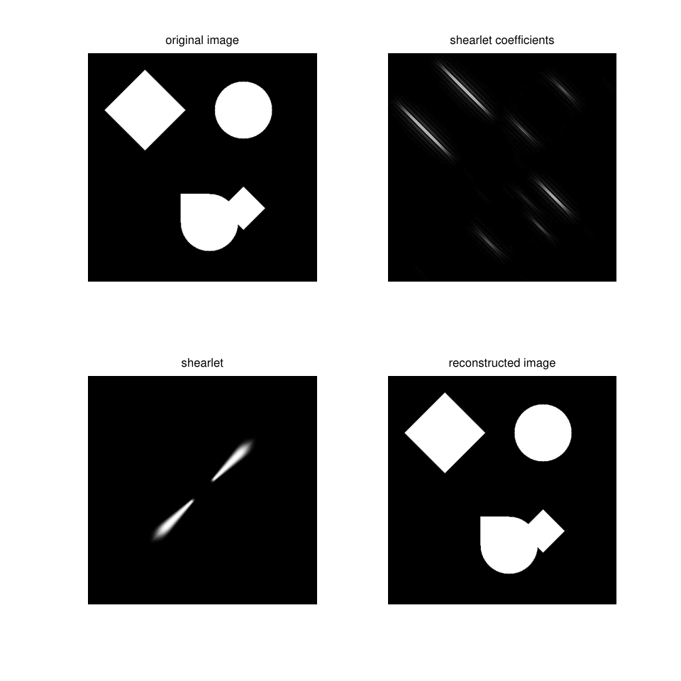
Refer to caption
Figure 14: Result of script simple_example.

3.6 Performance

To evaluate the performance and the exactness of our implementation we present the following figures: In Figure 15(a) we investigate the numerical tightness of the frame. The figure shows the difference between the square sum of the shearlets and 11, i.e.,

∑κ∈{h,v}∑j=0j0−1∑k=−2j2j|ψ^j,k,0κ|2+∑j=0j0−1∑k=±2j|ψ^j,k,0h×v|2+|ϕ^0|2−1.\sum_{\kappa\in\{h,v\}}\sum_{j=0}^{j_{0}-1}\sum_{k=-2^{j}}^{2^{j}}\lvert\hat{\psi}^{\kappa}_{j,k,0}\rvert^{2}+\sum_{j=0}^{j_{0}-1}\sum_{k=\pm 2^{j}}\lvert\hat{\psi}^{h\times v}_{j,k,0}\rvert^{2}+\lvert\hat{\phi}_{0}\rvert^{2}-1.

The largest deviation is about 8⋅10−158\cdot 10^{-15} which is 4040 times the machine precision. Figure 15(b) shows the difference between a random image and after transform and inverse transform, i.e., the exactness of the forward and backwards transform. Here the biggest difference is about 2⋅10−152\cdot 10^{-15} or approximately 10 times the machine precision. Surprisingly, this is even better than the tightness of the used frame.

Refer to caption ×10−15\times 10^{-15}22−2-244−4-466−6-688−8-800
((a)) Frame tightness.
Refer to caption ×10−15\times 10^{-15}0.50.5−0.5-0.511−1-11.51.5−1.5-1.522−2-200
((b)) Transform exactness.
Figure 15: Frame tightness and exactness of the implemented shearlet transform.

Most of the computation time is needed to precompute the spectra. Having the spectra the transform and the inverse can be computed efficiently. The running time of all mentioned implementations including ours is comparable but depends strongly on the used frequency tiling and thus of the oversampling factor.

3.7 Remarks

  1. (i)

    In [20] and the respective implementation ShearLab a pseudo-polar Fourier transform is used to implement a discrete (or digital) shearlet transform. For the dilation aa and shear ss the same discretization as before is used. But for the translation tt the authors set tj,k,m:=Aaj,12​Ssj,k​mt_{j,k,m}:=A_{a_{j},\frac{1}{2}}S_{s_{j,k}}m where we in contrast simply set tm:=mt_{m}:=m (see (19)). Thus, their discrete shearlet becomes

    ψ~^j,k,m​(ω)=ψ^​(Aaj,12​Ssj,kT​ω)​e−2​π​i⁡⟨ω,Aaj,12​Ssj,k​m⟩=ψ^​(Aaj,12​Ssj,kT​ω)​e−2​π​i⁡⟨Ssj,kT​Aaj,12​ω,m⟩.\hat{\widetilde{\psi}}_{j,k,m}(\omega)=\hat{\psi}\left(A_{a_{j},\frac{1}{2}}S_{s_{j,k}}^{\text{\tiny$\operatorname{T}$}}\omega\right)\operatorname{e}^{-2\pi\operatorname{i}\bigl\langle\omega,A_{a_{j},\frac{1}{2}}S_{s_{j,k}}m\bigr\rangle}=\hat{\psi}\left(A_{a_{j},\frac{1}{2}}S_{s_{j,k}}^{\text{\tiny$\operatorname{T}$}}\omega\right)\operatorname{e}^{-2\pi\operatorname{i}\bigl\langle S_{s_{j,k}}^{\text{\tiny$\operatorname{T}$}}A_{a_{j},\frac{1}{2}}\omega,m\bigr\rangle}.

    Since the operation Ssj,kT​Aaj,12​ωS_{s_{j,k}}^{\text{\tiny$\operatorname{T}$}}A_{a_{j},\frac{1}{2}}\omega would destroy the pseudo-polar grid a “slight” adjustment is made and the exponential term is replaced by

    e−2πi⟨(θ∘Ssj,k−T)Ssj,kTAaj,12ω,m⟩\operatorname{e}^{-2\pi\operatorname{i}\bigl\langle\bigl(\theta\circ S_{s_{j,k}}^{-{\text{\tiny$\operatorname{T}$}}}\bigr)S_{s_{j,k}}^{\text{\tiny$\operatorname{T}$}}A_{a_{j},\frac{1}{2}}\omega,m\bigr\rangle}

    with θ:ℝ∖{0}×ℝ→ℝ×ℝ\theta\colon\mathbb{R}\setminus\{0\}\times\mathbb{R}\to\mathbb{R}\times\mathbb{R} and θ⁡(x,y)=(x,yx)\theta(x,y)=(x,\frac{y}{x}) such that

    e−2πi⟨(θ∘Ssj,k−T)Ssj,kTAaj,12ω,m⟩=e−2​π​i⁡⟨(aj​ω1,aj​ω2ω1),m⟩.\operatorname{e}^{-2\pi\operatorname{i}\bigl\langle\bigl(\theta\circ S_{s_{j,k}}^{-{\text{\tiny$\operatorname{T}$}}}\bigr)S_{s_{j,k}}^{\text{\tiny$\operatorname{T}$}}A_{a_{j},\frac{1}{2}}\omega,m\bigr\rangle}=\operatorname{e}^{-2\pi\operatorname{i}\bigl\langle\bigl(a_{j}\omega_{1},\sqrt{a_{j}}\frac{\omega_{2}}{\omega_{1}}\bigr),m\bigr\rangle}.

    With this adjustment the last step of the shearlet transform can be obtained with a standard inverse fast Fourier transform (similar as in our implementation). Unfortunately, this is no longer related to translations of the shearlets in time domain.

  2. (ii)

    We are aware of our larger oversampling factor in comparison with, e.g., ShearLab. Having four scales we obtain 61 images of the same size as the original image. But since shearlets are designed to detect edges in images we like to avoid any down-sampling and keep translation invariance. A possibility to reduce the memory usage is to use the compact support of the shearlets in the frequency domain and only compute them on a “relevant” region. This approach is called wrapping in [1] and used in the respective implementation of CurveLab. But we then also have to store the position and size of each region which decreases the memory savings and makes the implementation a lot more complicated.

3.8 Complex Shearlets

3.8.1 Guaranteeing Real Shearlet Coefficients

The inner product between two real-valued functions or vectors is again real-valued. However, when computing the shearlet coefficients in the way described above, we obtain complex coefficients for the finest scale if the image is of even length. Figure 18(a) shows the mean value of the absolute value of the imaginary part for direction in each scale (see Figure 13 for an explanation of these kind of figures). We clearly see that the imaginary part is non-zero for all non-axis aligned directions. The reason is that we destroy the intrinsic symmetry of the Fourier coefficients by cutting out the different parts of the Fourier spectra.

Figure 16: Symmetry of Fourier spectra. The dashed line is the order of the Fourier coefficients provided by Matlab. With fftshift we get the order marked by the solid lines. The point ∗* is an arbitrary point in the interior. Due to the symmetry it is complex conjugated to the point ∗¯\overline{*}. The same holds true for the points ∘\circ and ∘¯\overline{\circ} but they lie on the border of the spectrum.

In Figure 16 we sketch the Fourier coefficients of a real image of size N×NN\times N where NN is even. The dashed gray square in the lower right part is the output provided by Matlab. The zero coefficient is stored in the top left corner followed by the positive frequencies up to N2−1\frac{N}{2}-1 and then the negative frequencies from N2\frac{N}{2} to −1-1. By applying fftshift the frequencies are swapped such that we obtain the black solid square. Since the Fourier coefficients are NN-periodic this can also be seen as shifting the window through the periodic Fourier coefficients.

The Fourier coefficients are symmetric in the following sense: Take for example the point symbolized by ∗*. It has the same real part as the point marked with ∗¯\overline{*} but with negative imaginary part, i.e., they are complex conjugated. This holds true for most of the points.

The only points where one has to be careful are those in the first column and the first row since they do not have a corresponding symmetry point. As an example we take the point symbolized by ∘\circ. Due to the periodicity of the coefficients ∘\circ appears in the first column but also in the column N2\frac{N}{2} that does not belong to the image (it only has length NN). But by symmetry the point marked by ∘¯\overline{\circ} has to be complex conjugated to ∘\circ.

By applying the differently oriented (not horizontal or vertical) shearlets we cut out only one of the points ∘\circ or ∘¯\overline{\circ} such that we loose the symmetry. When we now apply the inverse Fourier transform we get complex shearlet coefficients.

We propose the following strategy to circumvent this effect: we modify the shearlets on the finest scale slightly to keep the symmetry. Roughly spoken we take the first column (respectively row) of the spectrum of shearlets and mirror it around the central zero axis. A complex conjugation is not necessary since we consider only real-valued spectra. To keep a frame we multiply them by 12\frac{1}{\sqrt{2}}. Figure 17 illustrates this. Note that the vertical and horizontal shearlet are kept unchanged.

8 6 4 2 0 0 0 0 0
((a)) Example first row.

12×\frac{1}{\sqrt{2}}\ \times\ 88 66 44 22 00 22 44 66 88

((b)) First row after mirroring and multiplying by 12\frac{1}{\sqrt{2}}.
Figure 17: Toy example to illustrate the adjustments to obtain real shearlet spectra.

When we now multiply the complex Fourier coefficients of the given image with the modified spectra, the symmetry is kept. This leads to real-valued shearlet coefficients or at least to an negligible imaginary part, see Figure 18(b).

((a)) Mean value of absolute value of the imaginary part of the shearlet coefficients over translations for each scale and shear.
((b)) Mean value of absolute value of the imaginary part of the shearlet coefficients over translations for each scale and shear after applying the above described modification.
Figure 18: Imaginary part of shearlet coefficients.
Remark 3.3.

Since for odd-sized images the symmetry is always kept, it is also possible to extend the Fourier coefficients by mirroring for even-sized images. But then a FFT of an odd-sized image has to be computed which is in general significantly slower than the one of an even-sized image.

3.8.2 Complex Shearlets and Shearlet Coefficients

In some situations one actually wants complex shearlets and complex coefficients, in particular for the analysis of the phase of the coefficients (and not only the absolute value).

With our construction complex shearlets (and thus complex shearlet coefficients) can be build straightforward. We obtain complex shearlets in time domain by considering one-sided shearlets in frequency domain, see Figure 19. The resulting shearlets in time domain are shown with their real and imaginary part in Figure 20. The computations and frame properties are the same as in the real-valued case.

Refer to caption
Figure 19: One-sided shearlet in Fourier domain.
Refer to caption
((a)) Real part of complex shearlet in time domain.
Refer to caption
((b)) Imaginary part of complex shearlet in time domain.
Refer to caption
((c)) 3D-view of real part of complex shearlet in time domain.
Refer to caption
((d)) 3D-view of imaginary part of complex shearlet in time domain.
Figure 20: Complex shearlet in time domain.

Acknowledgement

The first author thanks Tomas Sauer (University of Gießen) for his support at the beginning of this project.

References

  • [1] E. J. Candès, L. Demanet, D. L. Donoho, and L. Ying. Fast discrete curvelet transforms. Multiscale modeling and simulation, 5(3):861–899, 2006.
  • [2] O. Christensen. An Introduction to Frames and Riesz Bases. Birkhäuser Boston, 2003.
  • [3] F. Colonna, G. R. Easley, K. Guo, and D. Labate. Radon transform inversion using the shearlet representation. Applied and Computational Harmonic Analysis, 29(2):232–250, 2010.
  • [4] S. Dahlke, G. Kutyniok, P. Maass, C. Sagiv, H.-G. Stark, and G. Teschke. The uncertainty principle associated with the continuous shearlet transform. International Journal on Wavelets Multiresolution and Information Processing, 6(2):157–181, 2008.
  • [5] S. Dahlke, G. Kutyniok, G. Steidl, and G. Teschke. Shearlet coorbit spaces and associated Banach frames. Applied and Computational Harmonic Analysis, 27(2):195–214, 2009.
  • [6] Z. Dan, X. Chen, H. Gan, and C. Gao. Locally adaptive shearlet denoising based on bayesian MAP estimate. In Proceedings of 6th International Conference on Image and Graphics (ICIG), pages 28–32, Hefei, China, 2011.
  • [7] D. L. Donoho and G. Kutyniok. Geometric Separation using a Wavelet-Shearlet Dictionary. In L. Fesquet and B. Torrésani, editors, Proceedings of 8th International Conference on Sampling Theory and Applications (SampTA), Marseille, 2009.
  • [8] G. R. Easley, F. Colonna, and D. Labate. Improved radon based imaging using the shearlet transform. In H. H. Szu and F. J. Agee, editors, Proceedings of Independent Component Analyses, Wavelets, Neural Networks, Biosystems, and Nanoengineering VII, volume 7343 of Proc. SPIE, Orlando, Florida, 2009.
  • [9] G. R. Easley and D. Labate. Image Processing using Shearlets. In G. Kutyniok and D. Labate, editors, Shearlets: Multiscale Analysis for Multivariate Data, pages 283–325. Birkhäuser Boston, 2012.
  • [10] G. R. Easley, D. Labate, and F. Colonna. Shearlet-based total variation diffusion for denoising. IEEE Transactions on Image Processing, 18(2):260–268, 2009.
  • [11] G. R. Easley, D. Labate, and W.-Q. Lim. Sparse directional image representations using the discrete shearlet transform. Applied and Computational Harmonic Analysis, 25(1):25–46, 2008.
  • [12] G. R. Easley, V. M. Patel, and D. M. Healy. Inverse halftoning using a shearlet representation. In V. K. Goyal, M. Papadakis, and D. van de Ville, editors, Proceedings of Wavelets XIII, volume 7446 of Proc. SPIE, San Diego, 2009.
  • [13] K. Guo, G. Kutyniok, and D. Labate. Sparse multidimensional representations using anisotropic dilation and shear operators. In G. Chen and M.-J. Lai, editors, Proceedings of Wavelets und Splines, pages 189–201, Athens, USA, 2006. Nashboro Press.
  • [14] K. Guo and D. Labate. The construction of smooth Parseval frames of shearlets. Mathematical Modelling of Natural Phenomena, 8(1):82–105, 2013.
  • [15] S. Häuser. Shearlet Coorbit Spaces, Shearlet Transforms and Applications in Imaging. Dissertation, TU Kaiserslautern, 2014.
  • [16] S. Häuser and G. Steidl. Convex multiclass segmentation with shearlet regularization. International Journal of Computer Mathematics, 90(1):62–81, 2013.
  • [17] E. J. King, G. Kutyniok, and W.-Q. Lim. Image inpainting: theoretical analysis and comparison of algorithms. In D. Van De Ville, V. K. Goyal, and M. Papadakis, editors, Proceedings of Wavelets and Sparsity XV, volume 8858 of Proc. SPIE, San Diego, 2013.
  • [18] G. Kutyniok, W.-Q. Lim, and R. Reisenhofer. ShearLab 3D: faithful digital shearlet transforms based on compactly supported shearlets. Preprint, 2014.
  • [19] G. Kutyniok, M. Shahram, and D. L. Donoho. Development of a digital shearlet transform based on pseudo-polar FFT. In G. V. K., M. Papadakis;, and D. van de Ville, editors, Proceedings of Wavelets XIII, volume 7446 of Proc. SPIE, San Diego, 2009.
  • [20] G. Kutyniok, M. Shahram, and X. Zhuang. ShearLab: A rational design of a digital parabolic scaling algorithm. SIAM Journal on Imaging Sciences, 5(4):1291–1332, 2012.
  • [21] W.-Q. Lim. The discrete shearlet transform: a new directional transform and compactly supported shearlet frames. IEEE Transactions on Image Processing, 19(5):1166–1180, 2010.
  • [22] W.-Q. Lim, G. Kutyniok, and X. Zhuang. Digital shearlet transforms. In G. Kutyniok and D. Labate, editors, Shearlets: Multiscale Analysis for Multivariate Data, pages 239–282. Birkhäuser Boston, 2012.
  • [23] J. Ma and G. Plonka. A review of curvelets and recent applications. IEEE Signal Processing Magazine, 27(2):118–133, 2010.
  • [24] S. Mallat. A Wavelet Tour of Signal Processing: The Sparse Way. Academic Press, 2008.
  • [25] Y. Meyer. Oscillating Patterns in Image Processing and Nonlinear Evolution Equations. AMS, 2001.
  • [26] V. M. Patel, G. R. Easley, and D. M. Healy. Shearlet-based deconvolution. IEEE Transactions on Image Processing, 18(12):2673–2685, 2009.