Optimization in Multi-Frequency Interferometry Ranging: Theory and Experiment

Existing works have shown the UMR of some specially designed frequency patterns. Equally spaced frequency is employed in RIPS (Radio Interferometric Positioning System) [2] and the UMR is the synthetic wavelength of adjacent frequency, i.e. $c/\Delta f$. In [4], the geometric series of wavelengths is used and the UMR is extended to the synthetic wavelength of the closest two frequencies or the largest synthetic wavelength. The beat wavelength coincidence method is adopted in [23] and the UMR is further enlarged by a factor of positive integer relative to that of [4].

Meanwhile, ranging accuracy of multi-frequency interferometry system is another important target to be optimized. However, there exists limited works concerned with the accuracy improvement by frequency optimization as well as the performance analysis of ranging error in the literature.

Among them, the estimation accuracy of RIPS method is in proportion to frequency separation, while the UMR is in inverse proportion to frequency separation[1][2]. Then, there exists a compromise between the accuracy and UMR in RIPS. The multistage beat wavelength method is exploited for range estimation and frequency design in [4] [23]. The measurement phase noise will be amplified by $\Lambda_{0i}/\Lambda_{0,i+1}$ when two neighbor synthetic wavelengths $\Lambda_{0i}$, $\Lambda_{0,i+1}$ are used for phase unwrapping (determine the integer number of wavelength) in each stage. In order to maximize noise immunity, the wavelength ratio should be equal and the phase noise will be uniformly amplified in each stage. With this in mind, a geometric series of wavelengths is formed[4]. However, the optimization criterion of [4][23] is built on the beat wavelength method. Although it is a fast estimation method, it is far from the optimal one in term of estimation accuracy since only partial information is used in each stage.

Note that similar problem arises in array design, that is, how to improve direction-of-arrival (DOA) estimation performance by optimizing the antenna positions of the $n$-element linear antenna array. The linear array geometry (antenna separation) design is most similar to our frequency pattern (frequency separation) design. So, we will also review the array geometry design of antenna array. The antenna positions are optimized to minimize the CRB of DOA estimation by numerical optimization in [3]. Based on the CRB principle, [11] also considers the linear array optimization problem for joint range and DOA estimation.

However, it seems not to be reasonable to optimize array geometry or frequency pattern only relying on CRB since it is a local measure of estimation accuracy. The ambiguity function is introduced when the global accuracy performance and the outlier are evaluated [11][12][16]$\sim$[19].

Nonuniform linear array optimization is discussed in [12] with emphasis on the comparison between uniform array, nonredundant array and minimum redundant array. Array geometry is optimized in [18] to minimize the outlier probability. For each given geometry, the ambiguity function reaches its minimal at a certain direction and the optimal array is the one with the minimal value maximized. Both CRB and the ambiguity function are used to optimize the two-dimension array in [19], and the genetic algorithm is adopted to search for the best array with the minimal CRB, under the constraint that the outlier probability is below a certain threshold.

Outlier or sidelobe suppression is also an important topic in step frequency radar. Due to extremely large bandwidth, the estimation accuracy is easily satisfied and more attention is paid to outlier suppression. To this end, random frequency step or different number of the frequency repetitions are proposed[30][31][32]. This is quite different from narrowband ranging. It is interesting to find in later section that the frequency pattern of our method is quite different from that in step frequency radar, where more weight is given to the frequencies distributed in the center instead of two ends of the band.

It is known that the theoretical rigorous UMR of MFI is the least common multiple (LCM) of all wavelengths when expressed as integers by quantization[5][14][21]. We prove that the UMR is the LCM of all synthetic wavelength of adjacent frequency or in inverse proportion to the greatest common divisor (GCD) of all frequency spacing when the initial frequency is properly chosen. Thus reducing the GCD will readily extend the measurement range. Compared with the wavelength-based method, the frequency spacing-based method can make full use of the band, in the sense that there have far more frequencies to be picked up for UMR extension within a given bandwidth[29]. What is more, with the initial frequency fixed, it is possible to adjust the order of the frequency spacing (known as permutation) to generate various set of measurement frequencies, maintaining the same UMR, since the GCD of all frequency spacing remains unchanged. This forms the key foundation of later MSE optimization via the permutation of frequency spacing. It is also pointed out that the rigorous UMR is overly optimistic in case of random initial frequency and a more practical expression for the UMR is derived.

The search based ambiguity function method is widely used to cope with the outlier in antenna array. However, it could not be directly applied to the MFI system because the obvious differences lie between the two systems. The parameter space of ambiguity function is “bounded” to the direction of $-180^{\circ}\sim 180^{\circ}$ for antenna array. It is not the case for MFI since the UMR will increase monotonously as the GCD of frequency spacing decreases. Moreover, constrained by the size and cost, the number of antenna is usually limited for array design while a large amount of frequencies may be required for accurate ranging in MFI. With this in mind, the ambiguity function of MFI is regarded as a theoretical foundation for the evaluation of a given frequency pattern or selecting the optimal frequency pattern from a very limited set. We also use the probability density function for analysis of the outlier probability and then design the frequency pattern with low outlier probability.

The relationship between the theoretical attainable ranging accuracy and the frequency pattern is the major issue of the paper. It is well known that the LS estimator exhibits a threshold effect, i.e., the MSE increases sharply below a certain SNR. Surprising, it is found that the LS estimator of MFI system shows a distinguished “double threshold effect”, especially for $f_{i}\gg B$. Distinctive difference is observed for the MSE in moderate and high SNR region (denoted by MMSE and HMSE respectively). Beside the conventional threshold effect caused by outlier in low-SNR region, another threshold effect occurs during the rapid transition from large MMSE to small HMSE with increased SNR (see Fig.5). The closed-form expression for the MMSE, HMSE and CRB are further obtained with HMSE coinciding with CRB. Under the assumption that $f_{i}\gg B$, which is true in most cases, different frequency design methods have almost the same HMSE and it is not the case for MMSE. Therefore, we focused on MMSE minimization by proper frequency optimization.

A quite simple prime-based frequency design method is finally developed with no need of searching. That is, if priori knowledge is provided and the range uncertainty can be restricted to the mainlobe region of cost function, i.e., the outlier is excluded, the optimal measurement frequency is proved to be densely distributed on both ends of the band. Otherwise, a prime-based frequency interval is firstly constructed for the purpose of both sidelobe suppression and UMR extension, followed by a special optimal rearrangement of the frequency interval. The proof of the optimal rearrangement is given for the first time, in the sense of MMSE minimization.

Different from the exhaust search or numerical optimization method, which have prohibitive computational complexity with increased antennas or measurement frequencies (Suppose $N$ measurement frequencies should be selected from $M$ possible frequencies, there exists $C_{M}^{N}$ combinations of measurement frequencies, so the antenna number $N=4$ is used in [18]), the proposed method may be free of the frequency number constraint. Moreover, for given bandwidth and frequency number, it is usually thought that the UMR and the ranging accuracy can not be improved simultaneously[28]. However, the proposed method and subsequent experiments have changed this opinion .

Apart from the simulation analysis, field experiment in outdoor non-Gaussian channel (multipath error is incorporated inevitably) is also performed. The experiment results demonstrate that the proposed scheme considerably outperforms the existing method in UMR as well as MSE performance. Meanwhile, the simplicity and robustness even to non-Gaussian error are also attractive for its practical use.

Notation: Upper (lower) bold face letters are used for matrices (column vectors). $\mathbf{E}[x]$, $|x|$, $\angle{[x]}$, $\mathbf{Re}\{x\}$ and $\mathbf{Im}\{x\}$ denote the operation of taking expectation, absolute value, phase angle, real part and imaginary part of $x$, respectively. $[x]_{2\pi}$ denotes modulo-$2\pi$ operation, which reduces $x$ to the interval $(-\pi,\pi]$. $\hat{x}$ and $x^{\ast}$ denotes the estimate and optimal solution of $x$. $\mathbf{I}_{N}$ denotes the $N\times N$ identity matrix; $\mathbf{1}_{N}$ denotes an $N\times 1$ all-one column vector; $j=\sqrt{-1}$ ; The mth row and nth column entry of matrix $\mathbf{A}$ are denoted as $\mathbf{A}(m,n)$ or $\mathbf{[A]}_{m,n}$. The trace of $\mathbf{A}$ is given as $\mathrm{tr}(\mathbf{A})=\sum_{m}\mathbf{A}(m,n)$. $(\cdot)^{T}$, $(\cdot)^{H}$ and $(\cdot)^{-1}$ denote matrix transpose, conjugate transpose and inverse operators, respectively. We use script letters $\mathcal{A}$ to define sets and by $|\mathcal{A}|$ its cardinality.

In the absence of noise, the measurement phase of multi-frequency interferometry ranging system is related to the range $q_{0}$ by the following equation[1][2][4][23]

where $\lambda_{i}=c/f_{i}$ is the wavelength of the carrier frequency $f_{i}$, and $c$ is the speed of light, $q_{0}$ is the true range (it is the q-range in radio interferometry and path length difference in optical interferometry)and $\varphi_{0}(i)$ is the ideal measurement phase wrapped to the principal interval of $(-\pi,\pi]$. The subscript “0” denotes the true or ideal value. Equation (1) is equivalent to

where $n_{i}$ is an unknown integer. For single measurement frequency, the range must satisfy $|q_{0}|<\lambda_{i}/2$ and then $q_{0}=\varphi(i)\lambda_{i}/{2\pi}$ with $n_{i}=0$. Otherwise, ambiguity appears because $n_{i}$ is undetermined. Therefore, multi-frequency ranging is usually needed.
There are various methods to estimate $q_{0}$ with a set of phase $\varphi(i)$ given, such as the CRT method [8][13][14], the LS-based search method [2], the modulo conversion method[10], the multistage unwrapping method[4][7][21][23], the excess fractions method[24]. Among which, the LS-based search method can achieve best estimation performance and will be adopted in the paper (we concentrate on the frequency design rather than estimation method), in the form of

where $S(q)$ denotes the cost function and $\varphi(i)$ is the measurement phase with phase error $\theta_{e}(i)$.

Before a formal derivation of the unambiguous range, we begins with an intuitive interpretation of the ambiguity problem.
Fig. 1 shows the relationship between theoretical and measurement phase without noise under different range $q$. The theoretical and measurement phase are represented by red lines and blue stars. Although the true range $q$ as well as the theoretical phase are different, the measurement phase are the same with $\Delta f=1.5\textrm{MHz}$. Note that the measurement phase is all the information we have in estimating $q$. In other words, the range $q=50$ and $q=250$ are indistinguishable for $\Delta f=1.5\textrm{MHz}$ and the ambiguity happens. If we measure the phase with a frequency spacing of $\Delta f=0.5\textrm{MHz}$ instead, the difference will immediately appear. This suggests that the ambiguity is closely related to the frequency spacing.

For multi-frequency interferometry ranging, the phase under $q+\Delta L$ and $q$ are given by

Ambiguity occurs if and only if the ranges $q$ and $q+\Delta L$ have the same phase in all measurement frequencies $f_{i},i=1,2,\cdots N$. That is,

Then

Where $n_{i}\in\mathbf{Z}$ and $\lambda_{i}$ is the wavelength of frequency $f_{i}$. Clearly, there are indefinitely many solutions of $\Delta L$ satisfying equation system in (5). Obviously, the minimum among those solutions is defined as the unambiguous measurement range (UMR). Equation (6) implies that the UMR is the least common multiple of all wavelengths[21].

To get closed-form solutions of $\Delta L$ in terms of frequency spacing instead of wavelength, equation system in (5) is transformed into an equivalent form as follows:

• •

  Condition 1: Equal initial phase at initial frequency $\hat{\varphi}_{q+\Delta L}(1)=\hat{\varphi}_{q}(1)$.

• •

  Condition 2: Equal phase increment between adjacent frequencies $\Delta\hat{\varphi}_{q}(i,i+1)=\Delta\hat{\varphi}_{q+\Delta L}(i,i+1)$.

where $\Delta\hat{\varphi}_{q}(i,j)=\left[\hat{\varphi}_{q}(j)-\hat{\varphi}_{q}(i)\right]_{2\pi}$.

From Condition 1, we get

From Condition 2, we get

where $\Delta f_{i}=f_{i+1}-f_{i}$ (assume $f_{1}<f_{2}<\cdots<f_{N}$) and $k_{0},k_{i}$ are positive integer.

Inspired by the result in [18][19], we introduce the ambiguity function to cope with the outlier (the wrong estimate lies outside the main lobe of the cost function) in multi-frequency interferometry ranging.

It is proved in [17] [19] that the outlier probability is in proportion to the ambiguity function

where

It is obvious that the ambiguity function attains its global maximal $1$ when $\Delta q=k\Delta L$, where $k$ is an integer. This kind of ambiguity (UMR) is inherent and inevitable. The UMR is excluded with the constraint $|q_{0}|<\Delta L$. Meanwhile, for $\frac{B_{m}}{2}<|\Delta q|<\Delta L-\frac{B_{m}}{2}$, $B_{m}$ is the width of mainpeak, there still exists the second maximal which may exceed the value achieved at the true $q_{0}$ with the help of noise and lead to large error, i.e., outlier. The objective is to solve the following optimization problem

Since

Then the problem becomes

Note that we are interested in those $\Delta q$ satisfying $\left[\frac{2\pi}{c}(f_{i}-f_{k})\Delta q\right]_{2\pi}\ll 1$ , which are prone to resulting in outlier. Using a first-order Taylor series expansion of $e^{x}$, we have

According to [6]

where

It becomes the max-mini optimization problem

When $N$ is large, it is approximated as

Note that (21) may be used to judge the quality of a specific $\Delta\mathbf{f}$ as well as to search for an optimal $\Delta\mathbf{f}$, in term of minimal outlier probability. As is the usual case in array design [18] [19]. However, we are not intended to find the optimal $\Delta\mathbf{f}$ by exhaust searching due to the formidable complexity when the parameter space is too large. It is known that the probability density function (PDF) of $q$ given $q_{0}$ and the measurement phase variance $\sigma_{\theta}^{2}$ at frequency $f_{i}$ is [21][25][28]

The joint probability density functions for measurement using two adjacent frequencies $f_{i}$ and $f_{i+1}$ becomes

When $f_{1}\gg B$, $\sigma_{q}(k)\approx\sigma_{q}(0)$, denoted as $\sigma_{q}$, (24) can be simplified as

Let $\Delta q=q-q_{0}$, it is proved in section II-B that the UMR is well approximated by $c/\Delta f_{i}$ for two adjacent frequencies $f_{i}$ , $f_{i+1}$ satisfying $f_{i}\gg(f_{i+1}-f_{i})$. So, $p(f_{i},f_{i+1}|q)$ is $c/\Delta f_{i}$-periodic functions ( $p(f_{i},f_{i+1}|q)=p(f_{i},f_{i+1}|q+kc/\Delta f_{i})$, $k\in\mathbf{Z}$, see Fig.2). Then, sharp peak will appear at $\Delta q^{(i)}(k)=kc/\Delta f_{i}$.
Denote $\mathbf{f}=[f_{1},f_{2},\cdots,f_{N}]$, the PDF for $N$ independent measurement frequencies is

(25) will be exploited in the design of $\Delta\mathbf{f}$ in later section.

Suppose the measurement phase at the $i\text{-th}$ frequency is $\varphi(i)=\left[2\pi q_{0}/\lambda_{i}+\theta_{e}(i)\right]_{2\pi}$, and the estimated phase is $\hat{\varphi}_{q}(i)=\penalty\left[2\pi q/\lambda_{i}\right]_{2\pi}$. where $q_{0}$, $q$ are the true and estimated range, $\theta_{e}(i)$ is assumed to be i.i.d white Gaussian noise. The LS-based objective function is given by

Since $\left[[x]_{2\pi}-[y]_{2\pi}\right]_{2\pi}=[x-y]_{2\pi}$, then (26) becomes

We will derive the MSE using the perturbation analysis approach[26]. The MSE for the moderate and high SNR are denoted by MMSE and HMSE in the paper. For SNR high enough, i.e., $\left|\Delta q\right|<\lambda_{N}\cdots<\lambda_{1}$. In this case, (27) may be simplified as

The optimal $\Delta q$ satisfy

Then the HMSE is readily obtained

For moderate or high SNR, $\left|\Delta q\right|>\lambda_{N}$, but $\left|\Delta q\right|<c/2B$, then the error could not be obtained directly. Similar to (17), we may transform the estimator into (since $\Delta q$ is the one minimizing (27), then it leads to small $({2\pi f_{i}\Delta q}/{c}-\theta_{e}(i))$ for moderate or high SNR):

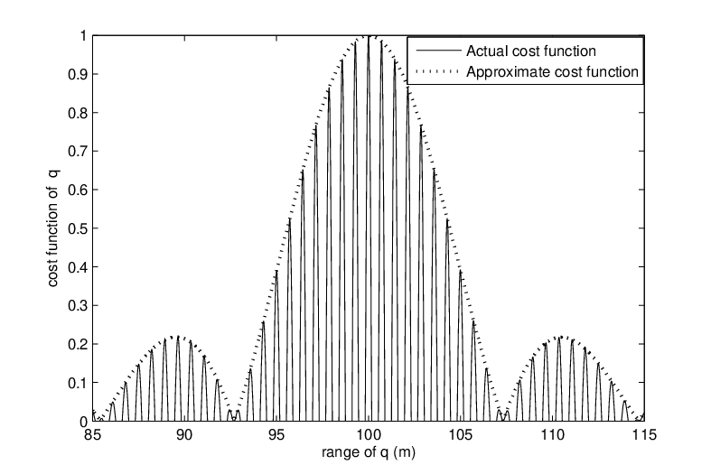
When $f_{1}/B\gg 1$, the problem may be well approximated as (the approximation is reasonable, as is confirmed in later simulation, see Fig.3 and Fig.5)

or equivalently

When $\left|\Delta q\right|<c/2B$, then $\left|\Delta q\right|<\left|c/2\left(f_{i}-f_{k}\right)\right|$. Omitting the influence of $\theta_{e}(i)-\theta_{e}(k)$ for moderate or high SNR, (33) can be rewritten as

Define

The problem can be expressed as

Where $\mathbf{R}^{-1}$, $\mathbf{R}$, $\mathbf{u}$ are defined in (19). The optimal solution obey

Since $\partial\left[\phi_{\Delta q}(i,1)\right]/\partial(\Delta q)=\penalty\frac{2\pi}{c}\left(f_{i}-f_{1}\right)=\penalty\frac{2\pi}{c}\sum_{k=1}^{i-1}{\Delta f_{k}}$, where $\Delta f_{k}=f_{k+1}-f_{k}$, and

It follows that

Then

Since

Therefore, the MMSE for this moderate SNR is given by

It is well known that the phase noise in (3) follows the wrapped normal distribution due to modulo $2\pi$ operation[27][28]. So the estimation is usually not unbias and the CRB does not exist. But the noise can be approximated as normal distribution under the assumption of high SNR.

Consider the signal $y(k)=e^{j2\pi q/\lambda_{k}}+n(k)$, where $q$ is the parameter to be estimated and $n(k)$ is the complex Gaussian noise with zero-mean and variance $\mathbf{E}[n^{2}(k)]=\sigma_{n}^{2}=\sigma^{2}$ and the signal-to-noise ratio (SNR) is defined as $\textrm{SNR}=1/\sigma^{2}$. The signal can be expressed as

Let $n^{\prime}(k)=n(k)e^{-j2\pi q/\lambda_{k}}=n^{\prime}_{R}(k)+n^{\prime}_{I}(k)j$, then $n^{\prime}(k)$ is statistically equivalent to $n(k)$ with $\mathbf{E}[n^{\prime 2}(k)]=\sigma^{2}$ and $\mathbf{E}[{n^{\prime}_{I}}^{2}(k)]={\sigma^{2}/2}$. Therefore

References

• [1] M. Maroti, B. Kusy, G. Balogh, P. Volgyesi, A. Nadas, K. Molnar, S. Dora, and A. Ledeczi, “Radio interferometric geolocation,” in Proc. of 3rd ACM International Conference on Embedded Networked Sensor Systems (SenSys), Nov. 2005.
• [2] B. Kusy, M. Maroti, G. Balogh, P. Volgyesi, J. Sallai, A. Nadas, A. Ledeczi, and L. Meertens, “Node density independent localization,” in Proc. of 5th International Symposium on Information Processing in Sensor Networks (IPSN/SPOTS), Apr. 2006.
• [3] A. B. Gershman and J. F. Böhme, “A Note on Most Favorable Array Geometries for DOA Estimation and Array Interpolation,” IEEE Signal Processing Lett., vol. 4, pp. 232-235, Aug. 1997.
• [4] C. E. Towers, D. P. Towers, J. D. C. Jones, “Optimum frequency selection in multifrequency interferometry,” Opt. Lett. vol.28, pp.887-889, Jun. 2003.
• [5] W. S. McCormick, J. B. Y. Tsui and V. L. Bakke, “A noise insensitive solution to an ambiguity problem in spectral estimation,” IEEE Trans. on AES, vol.25, pp.729-732, Sep. 1989.
• [6] Y. W. Wu, S. Rhodes and E. H. Satorius, “Direction of arrival estimation via extended phase interferometry,” IEEE Trans. on AES, vol.31, pp.375-380, Jan. 1995.
• [7] Y. Y. Cheng and J. C. Wyant, “Multiple-wavelength phase-shifting interferometry,” Appl. Opt, vol.24, pp. 804-807, Mar. 1985.
• [8] Z. Huang and Z. Wan, “Range ambiguity resolution in multiple PRF pulse Doppler radars,” in Proc. Int. Conf. Acoustics, Speech, Signal Processing (IEEE ICASSP), Dallas, TX, pp. 1786-1789, Apr. 1987.
• [9] P. Stoica and A. Nehorai, “MUSIC, maximum likelihood and Cramer-Rao bound,” IEEE Trans. Acoust., Speech., Signal Processing, vol. 37, pp. 720-741, May. 1989.
• [10] K. R. Sundaram, R. K. Mallik and U. M. S. Murthy, “Modulo conversion method for estimating the direction of arrival,” IEEE Trans. on AES, vol.36, pp.1391-1396, Oct. 2000.
• [11] M. I. Doroslovacki and E. G. Larsson, “Nonuniform linear antenna arrays minimizing Cramer-Rao bounds for joint estimation of single source range and direction of arrival,” IEE Proc., Radar Sonar Navig., vol. 152, pp.225-231, Aug. 2005.
• [12] E. J. Vertatschitsch, S. Haykin, “Impact of linear array geometry on direction-of-arrival estimation for a single source,” IEEE Trans. Antennas Propag. vol.39, pp.576-584, May. 1991.
• [13] X.-G. Xia and G. Wang, “Phase unwrapping and a robust Chinese remainder theorem,” IEEE Signal Process. Lett., vol. 14, no. 4, pp.247-250, Apr. 2007.
• [14] W. J. Wang and X.-G. Xia, “A closed-form robust Chinese remainder theorem and its performance analysis,” IEEE Trans. Signal Process, vol.58, pp.5655-5666, Nov. 2010.
• [15] S. Eilon and I. G. Chowdhury, “Minimizing waiting time variance in the single machine problem,” Manag. Sci. vol.23(6), pp.567-575, 1977.
• [16] A. Dogandzic and A. Nehorai, “Cramer-Rao bounds for estimating range, velocity, and direction with an active array,” IEEE Trans. Signal Processing, vol. 49, no. 6, pp. 1122-1137, Jun. 2001.
• [17] F. Athley, “Threshold region performance of maximum likelihood direction of arrival estimators,” IEEE Trans. Signal Process. vol.53, pp.1359-1373, Apr. 2005.
• [18] M. Gavish, A. J. Weiss, “Array geometry for ambiguity resolution in direction finding,” IEEE Trans. Antennas Propag. vol.44, pp.889-895, Jun. 1996.
• [19] T. Birinci, Y. Tanik, “Optimization of nonuniform array geometry for DOA estimation with the constraint on gross error probability,” Signal Processing, vol.87, pp.2360-2369, 2007.
• [20] D. C. Rife and R. R. Boorstyn, “Single-tone parameter estimation from discrete-time observations,” IEEE Trans. Inform. Theory, vol. IT-20, pp. 591-598, Sept. 1974.
• [21] I. Vrana, “Optimum statistical estimates in conditions of ambiguity,” IEEE Trans. Inform. Theory, vol.39. pp. 1023-1030, May. 1993.
• [22] L. Wei, W. D.  Qi, D. X.  Chen, P. Liu, E.  Yuan, “Optimal sequencing of a set of positive numbers with the variance of the sequence’s partial sums maximized,” Accepted for publication in Optimization Letter (DOI: 10.1007/s11590-012-0449-9), 2012.
• [23] K. Falaggis, D. P. Towers, and C. E. Towers, “Multiwavelength interferometry: extended range metrology,” Opt. Lett. vol.34, pp.950-952, Apr. 2009.
• [24] M. R. Benoit, “Application des phénomènes d’interférence à des déterminations métrologiques,” J. Phys. 3(7), 57-68, 1898.
• [25] V. Pascazio, and G. Schirinzi “Estimation of terrain elevation by multifrequency interferometric wide band SAR data,” IEEE Signal Processing Lett., vol. 8, pp. 7-9, Jan. 2001.
• [26] Y. T. Chan and K. C. Ho, “A simple and efficient estimator for hyperbolic location,” IEEE Trans. Signal Processing, vol. 42, pp. 1905-1915, Aug. 1994.
• [27] C. Bahlmann, “Directional features in online handwriting recognition,” Pattern Recog., vol. 39, pp. 115-125, 2006.
• [28] Y. Q. Cheng, X. Z. Wang, T. Caelli, and B. Moran, “Tracking and localizing moving targets in the presence of phase measurement ambiguities,” IEEE Trans. Signal Processing, vol. 59, pp. 3514-3525, Aug. 2011.
• [29] C. Wang, Q. Yin, and H. Chen, “Robust Chinese remainder theorem ranging method based on dual-frequency measurements,” IEEE Trans. Veh. Technol., vol. 60, pp. 4094-4099, 2011.
• [30] S. R. J. Axelsson,“Analysis of Random Step Frequency Radar and Comparison With Experiments,” IEEE Trans. Geosci. Remote Sens.,vol. 45, no. 4, pp. 890-904, Apr. 2007.
• [31] D. J. Rabideau, “Nonlinear synthetic wideband waveforms,” Proc. 2002 IEEE Radar Conf., pp.212-219, May. 2002.
• [32] N. Levanon,“Stepped-frequency pulse-train radar signal,” IEE Proc., Radar Sonar Navig., vol. 149, pp.297-309, Dec. 2002.
• [33] P. Liu, W. D.  Qi, E.  Yuan, Y. S. Zhu, H. Wang, “Ground displacement measurement by radio interferometric ranging for landslide early warning,” Instrumentation and Measurement Technology Conference (I2MTC), 2011 IEEE., May, 2011.