Sharp phase transition in
the random stirring model on trees Thanks: Dept. of Statistics, Oxford University. Supported by U.K. EPSRC grant EP/I004378/1.

Here we list alphabetically the notation which is commonly used in the article. A summarizing phrase is provided for each item, as well as the page number at which the concept is introduced.

As [2] mentions, on a regular tree, it is simple to see that, for each $t\in[0,\infty)$, there being positive probability that the cycle of $\phi$ under $\sigma_{t}$ is infinite is equivalent to the almost sure existence of some infinite cycle under $\sigma_{t}$.

Our analysis of the random stirring model exploits a closely related dependent random walk which was used in the proof of  [12, Theorem 1] and which was called the cyclic-time random walk in [2]. We now introduce some notation and define this walk.

For each edge $e\in E(\mathcal{T})$, the incident vertex of $e$ closer to $\phi$ will be called the parent vertex and will be denoted by $e^{+}$; the other, called the child vertex and labelled $e^{-}$.

For convenience, suppose that $\mathcal{T}$ is embedded in $\mathbb{R}^{2}$, so that each element of $V(\mathcal{T})$ is identified with a point in $\mathbb{R}^{2}$ and each element $e\in E(\mathcal{T})$ with the line segment $[v_{1},v_{2}]\subseteq\mathbb{R}^{2}$ where $e=(v_{1},v_{2})$ for $v_{1},v_{2}\in V(\mathcal{T})$. For each $v\in V(\mathcal{T})$, let the pole at $v$, $\{v\}\times[0,1)\subseteq\mathbb{R}^{3}$, denote the unit line segment that rises vertically from $v$. Elements of $E(\mathcal{T})\times[0,1)$ will be called bars. A bar $b=(e,h)$ is said to be supported on the edge $e$ and to have height $h$; we also record the edge on which $b$ is supported as $E(b)$. Note that the bar $(e,h)$ is a horizontal line segment which intersects the poles at $e^{+}$ and $e^{-}$; the intersection points $(e^{+},h)$ and $(e^{-},h)$ will be called the parent and child joints of $(e,h)$.

The bar set $E(\mathcal{T})\times[0,1)$ carries the product of counting and Lebesgue measure on its components. (As a shorthand, we will refer to this product measure simply as Lebesgue measure.)

Let $\mathcal{B}^{\prime}\subseteq E(\mathcal{T})\times[0,1)$ be a collection of bars which is locally finite in the sense that each $e\in E(\mathcal{T})$ supports only finitely many elements of $\mathcal{B}^{\prime}$. Cyclic-time random meander $X^{\mathcal{B}^{\prime}}_{(v,h)}:[0,\infty)\to V(\mathcal{T})\times[0,1)$, among $\mathcal{B}^{\prime}$ and with initial condition $(v,h)\in V(\mathcal{T})\times[0,1)$, is the following process. First, $X^{\mathcal{B}}_{(v,h)}(0)=(v,h)$; the process then rises at unit speed on the pole at $v$ until either it reaches $(v,1)$, when it jumps to $(v,0)$, or until it reaches the joint of a bar in $\mathcal{B}^{\prime}$, when it jumps to the other joint of this bar. After either of these events, $X^{\mathcal{B}^{\prime}}_{(v,h)}$ continues by iterating the same rule, until it is defined on all of $[0,\infty)$. The process is chosen to be right-continuous with left limits. Note that this choice implies that, if $(v,h)$ is the joint of a bar $b$ in $\mathcal{B}^{\prime}$, then $X^{\mathcal{B}^{\prime}}_{(v,h)}$ remains at the pole at $v$ at small times, rather than crossing $b$ at time zero. We abbreviate $X^{\mathcal{B}^{\prime}}$ for $X^{\mathcal{B}^{\prime}}_{(\phi,0)}$. (There are locally finite choices of $\mathcal{B}^{\prime}$ for which these rules fail to define $X^{\mathcal{B}^{\prime}}_{(v,t)}$ on all of $[0,\infty)$. It is a simple matter to verify that this difficulty does not arise in the case that is relevant to us and which we now discuss.)

Let $s\in(0,\infty)$. We will refer to the Poisson law on bar collections of density $s$ with respect to Lebesgue measure on $E(\mathcal{T})\times[0,1)$ as the Poisson-$s$ law. Let $\big\{\mathcal{B}_{s}:s\geq 0\big\}$ be a coupled collection of random bar collections, where $\mathcal{B}_{s}$ has the Poisson-$s$ law for each $s\in[0,\infty)$ and $\mathcal{B}_{s}\subseteq\mathcal{B}_{s^{\prime}}$ whenever $0\leq s<s^{\prime}<\infty$. Define $\sigma_{t}:V(\mathcal{T})\to V(\mathcal{T})$ by setting $\sigma_{t}(v)$ equal to the vertex component of $X^{\mathcal{B}_{t}}_{(v,0)}(1)$, and note that $\sigma_{t}$ is a random permutation of $V(\mathcal{T})$. With this notation, the random stirring process on $\mathcal{T}$ is the stochastic process, mapping $[0,\infty)$ to permutations of $V(\mathcal{T})$, given by $s\to\sigma_{s}$.

We now fix $t\in(0,\infty)$ and write $\mathbb{P}_{t}$ for a probability measure carrying a bar collection $\mathcal{B}\subseteq E(\mathcal{T})\times[0,1)$ having Poisson-$t$ law. Cyclic-time random meander with parameter $t$ is the random process $X^{\mathcal{B}}$.

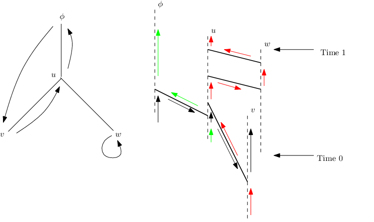
Cyclic-time random walk (begun at $\phi$) is the vertex-valued process given by projecting $X^{\mathcal{B}}:[0,\infty)\to V(\mathcal{T})\times[0,1)$ onto $V(\mathcal{T})$. (In fact, under our definition, cyclic-time random walk moves at a rate which is a factor of $t$ greater than it does under the definition in [2].) We will discuss cyclic-time random meander rather than walk, and will refer to $X^{\mathcal{B}}$ in shorthand as a meander. See Figure 1 for an illustration.

In 1953, Feynman [5] wrote the quantum-mechanical partition function for helium as a sum over the energy associated to certain interacting Brownian particles that may interchange their positions over a finite-time interval. He argued that the $\lambda$-transition undergone by the gas at low temperature is reflected by the appearance of large cycles in a measure on permutations naturally associated to this representation of the partition function.

The random stirring (or random interchange) model was introduced in [9]. In this model also, the conjectured phase transition to lengthy cycles has a physical importance, since it is intimately connected to the off-diagonal long-range order anticipated for the spin-$1/2$ isotropic quantum Heisenberg ferromagnet at very low temperature: Bálint Tóth in [12] gave a representation of the partition function for this ferromagnet in terms of the random stirring model. The lecture notes [6] contain an overview of this topic. The phase transition to infinite cycles proved in Theorem 1.1 is expected to have a counterpart for the Euclidean lattice $\mathbb{Z}^{d}$ for $d\geq 3$. The author learnt of this question first after it was posed by Bálint Tóth.

Recent mathematical progress on the random stirring model includes the resolution of Aldous’ conjecture identifying its spectral gap [4], and a formula for the probability that the random permutation consists of a single cycle [1].

The emergence of a giant component under percolation on the complete graph as the percolation parameter increases through values near $1/n$ has been intensively studied. Oded Schramm [11] showed that this transition is accompanied by the appearance of large-scale cycles in the associated random stirring model: in the composition of $(1+\varepsilon)n$ independent uniform transposition on a given $n$-set, there exists a giant component of edges transposed at least once, of some density $\theta(\varepsilon)\in(0,1)$; when the cycle lengths in this random permutation are normalized by $\theta(\varepsilon)n$ and listed in decreasing order, they converge in law to the Poisson-Dirichlet distribution with parameter one. Nathanaël Berestycki [3] has given a short proof that a cycle exists of size $\Theta(n)$ when $(1+\varepsilon)n$ transpositions are made.

For any given graph $G$ on which the random stirring model is well-defined, let $\mathscr{T}^{G}$ denote the set of $t>0$ such that the random stirring process on $G$ at parameter $t$ has infinite cycles almost surely. Note that $t\not\in\mathscr{T}^{G}$ unless the bond percolation on $G$ given by the set of edges that support at least one bar in $\mathcal{B}$ has an infinite component. As noted in [2], this implies that $\big[0,-\log\big(1-p_{c}(G)\big)\big)\cap\mathscr{T}^{G}=\emptyset$, where $p_{c}(G)$ denotes the critical value for bond percolation on $G$. Noting that $p_{c}(\mathcal{T})=d^{-1}$, we find that

if $d\geq 8$. The papers [2] and [8] provide two different approaches to proving the existence of infinite cycles in the random stirring process. Appendix $B$ in the arXiv version of [8] draws on these approaches to provide the following quantitative summary. See Figure 2 for an overview of which ranges of $t$ are handled by the two techniques.

In fact, our monotonicity result is valid on a slightly longer interval. We now record this other form, since it indicates more accurately the limit of the method; but we will not prove it, since the proof contains no new ideas.

Cyclic-time random meander $X^{\mathcal{B}}$ is the tool that we will use to prove Propositions 1.3. Let $p_{\infty}=p_{\infty}(t)$ denote the $\mathbb{P}_{t}$-probability that $(\phi,0)\not\in X^{\mathcal{B}}(0,\infty)$. Note that in the random stirring model at parameter $t$, the cycle of $\phi$ is infinite with probability $p_{\infty}(t)$.

We will prove Proposition 1.3 by establishing that $p_{\infty}:\big[0,d^{-1}+2d^{-2}\big]\to[0,1]$ is non-decreasing (for high enough $d$). To do so, we will work with local approximations $\{p_{n}:n\in\mathbb{N}\}$ for $p_{\infty}$. To define these, we need some notation for describing the graph $\mathcal{T}$. We pause to collect together such general notation.

Throughout, we write $|\cdot|$ to denote the cardinality of a set.

For $n\in\mathbb{N}$, let $H_{n}^{\mathcal{B}}\in[0,\infty]$ denote the hitting time $\inf\big\{s>0:X^{\mathcal{B}}(s)\in\mathcal{V}_{n}\times[0,1)\big\}$. Let $p_{n}=p_{n}(t)$ denote $\mathbb{P}_{t}(H_{n}^{\mathcal{B}}<\infty)$. Evidently, $p_{n}$ decreases pointwise to $p_{\infty}$. Note that $p_{0}=1$.

The tool for deriving Proposition 1.3 is now stated. The derivative of $p_{n}$ is expressed in terms of the mean effect on $\mathbb{P}_{t}(H_{n}^{\mathcal{B}}<\infty)$ caused by adding to $\mathcal{B}$ a single “uniformly” placed bar. The formula, which is an analogue for the Poisson process of Russo’s formula from percolation theory [7, Theorem 2.25], is proved in [13]; however, while Russo’s formula is often applied for monotone events in the context of percolation, the event $\big\{H_{n}^{\mathcal{B}}<\infty\big\}$ is by no means monotone. We give a short argument to establish the formula for the sake of completeness.

We will introduce several events in order to discuss this pivotality: the crossing, bottleneck and non-escape events, $\mathsf{C}_{n},\mathsf{BN}_{n}$ and $\mathsf{NoEsc}_{n}$. To keep formulas uncluttered, we will omit the $n$-dependence in denoting these events, as we will also for the pivotality events $\mathsf{P}^{+}_{n}$ and $\mathsf{P}^{-}_{n}$.

Here we record two simple observations regarding cyclic-time random meander.

We set $\tau=td$, and will often use $\tau$ in place of $t$ in the ensuing estimates. Note that the range of $t$-values that concerns us, $[d^{-1},d^{-1}+2d^{-2}]$, corresponds to $\tau\in[1,1+2d^{-1}]$, so that $\tau$ is a unit-order quantity. Our use of the notation $\tau$ will emphasise how our argument is perturbative in high $d$: for example, we will see that, up to $\tau$-dependent unit-order factors, $\mathbb{P}_{t}\big(\mathsf{P}^{+}\cap\mathsf{C}\cap\mathsf{BN}^{c}\big)$ is at least $d\tfrac{p_{n-1}}{|E(\mathcal{T}_{n})|}$, and $\mathbb{P}_{t}\big(\mathsf{P}^{-}\cap\mathsf{C}\cap\mathsf{BN}^{c}\big)$ is at most $\tfrac{p_{n-1}}{|E(\mathcal{T}_{n})|}$, so that $A_{1}$ in (3.2) is positive if $d$ is high enough.

We now state the two main estimates that will lead to Proposition 1.8.

We now apply the estimates in Propositions 3.1 and 3.2 to Lemma 1.7 in order to prove Proposition 1.8.

The proposition then follows from Lemma 1.7, (3.1) and $p_{n-1}\geq p_{n}$. ∎

It remains to prove Propositions 3.1 and 3.2. Sections 4 and 5 treat each of these estimates in turn.

References

• [1] Gil Alon and Gady Kozma. The probability of long cycles in interchange processes. Duke Math. J., 162(9):1567–1585, 2013.
• [2] Omer Angel. Random infinite permutations and the cyclic time random walk. In Discrete random walks (Paris, 2003), Discrete Math. Theor. Comput. Sci. Proc., AC, pages 9–16 (electronic). Assoc. Discrete Math. Theor. Comput. Sci., Nancy, 2003.
• [3] Nathanaël Berestycki. Emergence of giant cycles and slowdown transition in random transpositions and kk-cycles. Electr. J. Probab., 16:152–173, 2011.
• [4] Pietro Caputo, Thomas M. Liggett, and Thomas Richthammer. Proof of Aldous’ spectral gap conjecture. J. Amer. Math. Soc., 23(3):831–851, 2010.
• [5] Richard P. Feynman. Atomic theory of the λ\lambda-transition in helium. Phys. Rev., 91(6):1291–1301, 1953.
• [6] Christina Goldschmidt, Daniel Ueltschi, and Peter Windridge. Quantum Heisenberg models and their probabilistic representations. In Entropy and the quantum II, volume 552 of Contemp. Math., pages 177–224. Amer. Math. Soc., Providence, RI, 2011.
• [7] Geoffrey Grimmett. Percolation, volume 321 of Grundlehren der Mathematischen Wissenschaften [Fundamental Principles of Mathematical Sciences]. Springer-Verlag, Berlin, second edition, 1999.
• [8] Alan Hammond. Infinite cycles in the random stirring process on trees. Bulletin of the Institute of Mathematics Academia Sinica (New Series)., 8(1):85–104. With a further appendix: arXiv:1202.1319, 2013.
• [9] T. E. Harris. Nearest-neighbor Markov interaction processes on multidimensional lattices. Advances in Math., 9:66–89, 1972.
• [10] Jean-François Le Gall. Random trees and applications. Probab. Surv., 2:245–311, 2005.
• [11] Oded Schramm. Compositions of random transpositions. Israel J. Math., 147:221–243, 2005.
• [12] Bálint Tóth. Improved lower bound on the thermodynamic pressure of the spin 1/21/2 Heisenberg ferromagnet. Lett. Math. Phys., 28(1):75–84, 1993.
• [13] S. A. Zuev. Russo’s formula for Poisson point fields and its applications. Diskret. Mat., 4(3):149–160, 1992.