跳到论文正文
W Papers独立论文阅读器 arXiv:1202.1278 论文正文 计算阅读时间 · 0%
引用这篇论文根据当前论文元数据生成,正式投稿前建议核对。


License: arXiv.org perpetual non-exclusive license
arXiv:1202.1278v2 [hep-th] 04 Apr 2012

Nearly Kähler heterotic compactifications
with fermion condensates

Athanasios Chatzistavrakidis    Olaf Lechtenfeld    Alexander D. Popov
Abstract

We revisit AdS4 heterotic compactifications on nearly Kähler manifolds in the presence of HH-flux and certain fermion condensates. Unlike previous studies, we do not assume the vanishing of the supersymmetry variations. Instead we determine the full equations of motion originating from the ten-dimensional action, and subsequently we provide explicit solutions to them on nearly Kähler manifolds at first order in α′\alpha^{\prime}. The Bianchi identity is also taken into account in order to guarantee the absence of all anomalies. In the presence of HH-flux, which is identified with the torsion of the internal space, as well as of fermion condensates in the gaugino and dilatino sectors, new solutions are determined. These solutions provide a full classification of consistent backgrounds of heterotic supergravity under our assumptions. All the new solutions are non-supersymmetric, while previously known supersymmetric ones are recovered too. Our results indicate that fully consistent (supersymmetric or not) heterotic vacua on nearly Kähler manifolds are scarce, even on AdS4, and they can be completely classified.

ITP–UH–04/12

$Bethe Center for Theoretical Physics and Physikalisches Institut der Universität Bonn,
Nussallee 12, D-53115 Bonn, Germany

e-mail: than@th.physik.uni-bonn.de

†Institut für Theoretische Physik, Leibniz Universität Hannover
Appelstraße 2, 30167 Hannover, Germany

e-mail: lechtenf@itp.uni-hannover.de

×Centre for Quantum Engineering and Space-Time Research
Leibniz Universität Hannover
Welfengarten 1, 30167 Hannover, Germany

∗Bogoliubov Laboratory of Theoretical Physics, JINR
141980 Dubna, Moscow Region, Russia

e-mail: popov@theor.jinr.ru

1 Introduction

Calabi-Yau compactifications of string theory, despite their welcome features, suffer from the infamous moduli problem, the existence of flat directions in the four-dimensional potential corresponding to scalar fields which are not stabilized. The most plausible scenario which resulted from the attempts to resolve this problem was the introduction of fluxes, namely vacuum expectation values of the tensor fields of the theory along the compactification manifold. These fluxes typically lead to a deformation of the internal manifold away from the Calabi-Yau property and suggest the study of non-Kähler manifolds [1, 2].

Unlike type II string theories, where the plentitude of Ramond-Ramond fields offers considerable freedom in the introduction of internal fluxes, the heterotic string case is more restrictive. Indeed, in the heterotic string the only field which may acquire an expectation value is the three-form HH of the common NS sector of string theory. Moreover, this field satisfies a more restrictive Bianchi identity than in the type II case. However, apart from the above field, it was suggested that, due to some strong dynamics in the hidden sector, fermion bilinears may also acquire some vacuum expectation value, thus forming a condensate [3, 4]. From a Calabi-Yau perspective such condensates are related to supersymmetry breakdown. Supersymmetric AdS4 heterotic compactifications on non-Kähler manifolds with fluxes and gaugino condensation were studied in [5, 6]. Moreover, a study including dilatino condensation was performed in [7]. However, the above studies do not deal with the solution of the equations of motion of the theory but only with the Killing spinor equations and the Bianchi identity. Nevertheless, according to Ivanov [8], it is not straightforward that the solution of the latter imply that the field equations are satisfied. Therefore it is more natural to directly investigate solutions of the field equations of the theory, whether supersymmetric or not. Such a perspective was employed in [9] where two such solutions were described, a supersymmetric one with fluxes and gaugino condensation and a non-supersymmetric one without gaugino condensation.

In the present paper we extend the analysis of [9] by implementing dilatino condensates into the theory. Working at first order in α′\alpha^{\prime}, we consider the heterotic string including four-fermion terms in the action and the supersymmetry variations. Varying this action, the corresponding equations of motion are determined. Assuming as background a product of four-dimensional AdS4 spacetime with a nearly Kähler internal space, all solutions to these equations are derived for two different choices of the connection on the tangent bundle. The Bianchi identity is also taken into account in order to guarantee the absence of all anomalies. An important feature of our investigation, motivated by the results of [8], is that the gauge field is taken to be a generalized instanton. Although it is in principle possible to consider non-instanton solutions, gauge fields enjoying the instanton property are distinguished by their immediate assurance for the fulfillment of the Yang-Mills equations. Apart from the solutions which were obtained in [9], our analysis reveals five sets of new non-supersymmetric solutions. Thus a classification of all possible nearly Kähler heterotic compactifications with torsion and fermion condensates is provided.

The paper is organized as follows. In Section 2 we present the action and the Killing spinor equations of the field theory limit of the heterotic string at first order in α′\alpha^{\prime}, retaining four-fermion terms involving the gaugino and the dilatino. Subsequently we determine the field equations resulting from this action and their decomposition according to the spacetime factorization AdS4×K{}_{4}\times K, where KK is a compact internal space of positive curvature. In Section 3 we briefly describe the geometry of nearly Kähler manifolds as far as it is needed in our investigation. Section 4 takes KK to be one of the four known compact homogeneous six-dimensional nearly Kähler manifolds and performs a systematic analysis of possible solutions of the field equations. We also check which of these solutions preserve supersymmetry. Finally, in Section 5 our results are summarized in three tables, which present the geometrical and field data as well as the fermion masses for all solutions, while some interesting properties are discussed as well.

2 Heterotic strings with fermion condensates

Field content, action and supersymmetry.

The low-energy field theory limit of heterotic string theory is given by d=10d{=}10, 𝒩=1{\cal N}{=}1 supergravity coupled to a super-Yang-Mills multiplet and it is defined on the 10dd spacetime MM. The supergravity multiplet consists of the graviton gg, which is a metric on MM, the left-handed Rarita-Schwinger gravitino ψ\psi, the Kalb-Ramond two-form field BB, the scalar dilaton ϕ\phi and the right-handed Majorana-Weyl dilatino λ\lambda. Moreover, the vector supermultiplet consists of the gauge field one-form AA and its superpartner, the left-handed Majorana-Weyl gaugino χ\chi.

Rather than presenting the full action describing the propagation and interactions of the above fields [10, 11], we shall restrict on the part which is relevant for our purposes. In this paper we shall consider vacuum solutions where the fermionic expectation values are zero, which is equivalent to the requirement of Lorentz invariance, but certain fermionic bilinears acquire non-trivial vacuum expectation values. However, these vacuum expectation values will not involve the gravitino and therefore it is consistent to set the gravitino to zero from the very beginning, ψ=0\psi=0. Then, in the string frame, the low-energy action up to and including terms of order α′\alpha^{\prime} reads as [12] 11 1 Comparing to the action which appears in [12], here we have made the following field redefinitions: ϕ→e2​ϕ/3\phi\rightarrow e^{2\phi/3}, χ→2​χ\chi\rightarrow\sqrt{2}\chi and H→13​2​HH\rightarrow{\textstyle\frac{1}{3\sqrt{2}}}H.

𝒮⁡(g,ϕ,B,χ,A)=∫Md10​x​detg​e−2​ϕ\displaystyle\mathcal{S}(g,\phi,B,\chi,A)=\int_{M}\!\!d^{10}x\ \sqrt{\det g}\ e^{-2\phi}\!\!\! {Scal+4|dϕ|2−12|H|2+12(H,Σ)−2(H,Δ)+14(Σ,Δ)−18|Σ|2+\displaystyle\!\!\!\Big\{{\text{Scal}}+4|d\phi|^{2}-{\textstyle\frac{1}{2}}|H|^{2}+{\textstyle\frac{1}{2}}(H,\Sigma)-2(H,\Delta)+{\textstyle\frac{1}{4}}(\Sigma,\Delta)-{\textstyle\frac{1}{8}}|\Sigma|^{2}+
+14α′tr(|R~|2−|F|2−2χ¯𝒟χ−13χ¯γMγA​BFA​BγMλ)+8λ¯𝒟λ},\displaystyle\ +\ {\textstyle\frac{1}{4}}\alpha^{\prime}\text{tr}\big(|\tilde{R}|^{2}-|F|^{2}-2\overline{\chi}\mathcal{D}\chi-{\textstyle\frac{1}{3}}\overline{\chi}\gamma^{M}\gamma^{AB}F_{AB}\gamma_{M}\lambda\big)+8\overline{\lambda}\mathcal{D}\lambda\Big\},

where capital Latin indices run from 0 to 9. Let us make clear the quantities and the notation in the above action. Scal is the curvature scalar, while the curvature forms FF and HH are defined as

F=d​A+A∧AandH=d​B+14​α′​[ωC​S​(Γ~)−ωC​S​(A)],F\ =\ dA+A\wedge A\qquad\text{and}\qquad H\ =\ dB+{\textstyle\frac{1}{4}}\alpha^{\prime}\big[\omega_{CS}(\tilde{\Gamma})-\omega_{CS}(A)\big], (2.2)

where ωC​S\omega_{CS} denotes the Chern-Simons-forms

ωC​S​(Γ~)=tr​(R~∧Γ~−23​Γ~∧Γ~∧Γ~)andωC​S​(A)=tr​(F∧A−23​A∧A∧A),\omega_{CS}(\tilde{\Gamma})\ =\ \text{tr}\big(\tilde{R}\wedge\tilde{\Gamma}-{\textstyle\frac{2}{3}}\tilde{\Gamma}\wedge\tilde{\Gamma}\wedge\tilde{\Gamma}\big)\qquad\text{and}\qquad\omega_{CS}(A)\ =\ \text{tr}\big(F\wedge A-{\textstyle\frac{2}{3}}A\wedge A\wedge A\big), (2.3)

and Γ~\tilde{\Gamma} is a connection on the tangent bundle T​MTM, whose choice is ambiguous. This connection could be chosen for example to be the Levi-Civita one, ΓLC​(g)\Gamma^{\text{LC}}(g), or a modified connection such as the plus or minus ones, Γ±=ΓLC∓12​H\Gamma^{\pm}=\Gamma^{\text{LC}}\mp{\textstyle\frac{1}{2}}H. We shall return to this point later in our analysis. The chosen connection determines the space-time curvature two-form

R~=d​Γ~+Γ~∧Γ~.\tilde{R}\ =\ d\tilde{\Gamma}+\tilde{\Gamma}\wedge\tilde{\Gamma}. (2.4)

Furthermore, in (2) appear the following expressions

tr​|R~|2=12​R~M​N​P​Q​R~M​N​P​Qandtr​|F|2=12​tr​FM​N​FM​N,\text{tr}|\tilde{R}|^{2}\ =\ {\textstyle\frac{1}{2}}\tilde{R}_{MNPQ}\tilde{R}^{MNPQ}\qquad\text{and}\qquad\text{tr}|F|^{2}\ =\ {\textstyle\frac{1}{2}}\text{tr}F_{MN}F^{MN}, (2.5)

and traces are taken over the adjoint representation of the gauge group or of SO(9,1), depending on the context. For any two pp-forms α,β\alpha,\beta we use the definitions

(α,β):=1p!​αM1​M2​…​Mp​βM1​M2​…​Mp,|α|2:=(α,α).(\alpha,\beta):=\frac{1}{p!}\alpha_{M_{1}M_{2}...M_{p}}\beta^{M_{1}M_{2}...M_{p}},\qquad|\alpha|^{2}:=(\alpha,\alpha). (2.6)

𝒟=γM​∇M\mathcal{D}=\gamma^{M}\nabla_{M} denotes the Dirac operator, coupled to ΓLC​(g)\Gamma^{\text{LC}}(g) and to AA. Finally, we have defined the fermion bilinears

Σ=124​α′​tr​(χ¯​γM​γN​γP​χ)​d​xM∧d​xN∧d​xP\Sigma\ =\ {\textstyle\frac{1}{24}}\alpha^{\prime}\,\text{tr}(\overline{\chi}\gamma_{M}\gamma_{N}\gamma_{P}\chi)\ dx^{M}\wedge dx^{N}\wedge dx^{P} (2.7)

and

Δ=16​(λ¯​γM​γN​γP​λ)​d​xM∧d​xN∧d​xP.\Delta\ =\ {\textstyle\frac{1}{6}}\,(\overline{\lambda}\gamma_{M}\gamma_{N}\gamma_{P}\lambda)\ dx^{M}\wedge dx^{N}\wedge dx^{P}. (2.8)

The action (2) is invariant under 𝒩=1{\cal N}{=}1 supersymmetry transformations [12], which act on the fermions as

δ​ψM\displaystyle\delta\psi_{M} =∇Mε−18​HM​N​P​γN​γP​ε+196​γ​(Σ)​γM​ε,\displaystyle\ =\ \nabla_{M}\varepsilon-{\textstyle\frac{1}{8}}H_{MNP}\gamma^{N}\gamma^{P}\varepsilon+{\textstyle\frac{1}{96}}\gamma(\Sigma)\gamma_{M}\varepsilon,
δ​λ\displaystyle\delta\lambda =−24​γ​(d​ϕ−112​H−148​Σ+148​Δ)​ε,\displaystyle\ =\ -{\textstyle\frac{\sqrt{2}}{4}}\gamma\big(d\phi-{\textstyle\frac{1}{12}}H-{\textstyle\frac{1}{48}}\Sigma+{\textstyle\frac{1}{48}}\Delta\big)\varepsilon, (2.9)
δ​χ\displaystyle\delta\chi =−14​γ​(F)​ε+ε​χ¯​λ−χ​ε¯​λ+γM​λ​χ¯​γM​ε,\displaystyle\ =\ -{\textstyle\frac{1}{4}}\gamma(F)\varepsilon+\varepsilon\overline{\chi}\lambda-\chi\overline{\varepsilon}\lambda+\gamma^{M}\lambda\overline{\chi}\gamma_{M}\varepsilon,

where ε\varepsilon is the supersymmetry generator, which is a left-handed Majorana-Weyl spinor. In addition, γ\gamma denotes the map from forms to the Clifford algebra,

γ⁡(1p!​ωM1​…​Mp​d​xM1∧⋯∧d​xMp)=ωM1​…​Mp​γM1​…​γMp.\gamma\big({\textstyle\frac{1}{p!}}\omega_{M_{1}\dots M_{p}}\ dx^{M_{1}}\wedge\dots\wedge dx^{M_{p}}\big)\ =\ \omega_{M_{1}\dots M_{p}}\gamma^{M_{1}}\dots\gamma^{M_{p}}. (2.10)

The following additional remarks concerning fermion bilinears are in order. The term in the action which is proportional to χ¯​γM​γA​B​FA​B​γM​λ\overline{\chi}\gamma^{M}\gamma^{AB}F_{AB}\gamma_{M}\lambda will be ignored in the following. This is a legitimate choice once we assume that there is no vacuum expectation value related to bilinears of the mixed form χ¯​λ\overline{\chi}\lambda and the like. Such a choice leads also to a further simplification of the gaugino supersymmetry transformation, which simply becomes

δ​χ=−14​γ​(F)​ε.\delta\chi\ =\ -{\textstyle\frac{1}{4}}\gamma(F)\varepsilon. (2.11)

Field equations.

The equations of motion may be obtained by varying the action (2), and they take the form (we symmetrize with weight one)

RicM​N+2(∇dϕ)M​N−18(H−12Σ+2Δ)P​Q​(MCLOSEHOPENN)P​Q++14​α′​[R~M​P​Q​R​R~NP​Q​R−tr​(FM​P​FNP+12​χ¯​γ(MCLOSE​∇OPENN)χ)]+2​λ¯​γ(MCLOSE​∇OPENN)λ=0,Scal−4​Δ​ϕ+4​|d​ϕ|2−12​|H|2+12​(H,Σ)−2​(H,Δ)+14​(Σ,Δ)−18​|Σ|2++14​α′​tr​[|R~|2−|F|2−2​χ¯​𝒟​χ]+8​λ¯​𝒟​λ=0,(𝒟−124​γ​(H−12​Σ+12​Δ))​(e−2​ϕ​χ)=0,(𝒟−124​γ​(H−18​Σ))​(e−2​ϕ​λ)=0,e2​ϕd∗(e−2​ϕF)+A∧∗F−∗F∧A+∗(H−12Σ+2Δ)∧F=0,d∗e−2​ϕ​(H−12​Σ+2​Δ)=0.\displaystyle\begin{aligned} \text{Ric}_{MN}+2(\nabla d\phi)_{MN}-{\textstyle\frac{1}{8}}(H-{\textstyle\frac{1}{2}}\Sigma+2\Delta)_{PQ(M}{H_{N)}}^{PQ}+\qquad\qquad\qquad\qquad\qquad\qquad\qquad\qquad\\ +{\textstyle\frac{1}{4}}\alpha^{\prime}\Big[\tilde{R}_{MPQR}{\tilde{R}_{N}}^{\ PQR}-\text{tr}\big(F_{MP}{F_{N}}^{P}+{\textstyle\frac{1}{2}}\overline{\chi}\gamma_{(M}\nabla_{N)}\chi\big)\Big]+2\overline{\lambda}\gamma_{(M}\nabla_{N)}\lambda&=0,\\ \text{Scal}-4\Delta\phi+4|d\phi|^{2}-{\textstyle\frac{1}{2}}|H|^{2}+{\textstyle\frac{1}{2}}(H,\Sigma)-2(H,\Delta)+{\textstyle\frac{1}{4}}(\Sigma,\Delta)-{\textstyle\frac{1}{8}}|\Sigma|^{2}+\qquad\qquad\qquad\qquad\quad\\ +{\textstyle\frac{1}{4}}\alpha^{\prime}\text{tr}\Big[|\tilde{R}|^{2}-|F|^{2}-2\overline{\chi}\mathcal{D}\chi\Big]+8\overline{\lambda}\mathcal{D}\lambda&=0,\\[2.0pt] \big(\mathcal{D}-{\textstyle\frac{1}{24}}\gamma(H-{\textstyle\frac{1}{2}}\Sigma+{\textstyle\frac{1}{2}}\Delta)\big)\big(e^{-2\phi}\chi\big)&=0,\\[4.0pt] \big(\mathcal{D}-{\textstyle\frac{1}{24}}\gamma(H-{\textstyle\frac{1}{8}}\Sigma)\big)\big(e^{-2\phi}\lambda\big)&=0,\\[4.0pt] e^{2\phi}d\ast(e^{-2\phi}F)+A\wedge\ast F-\ast F\wedge A+\ast(H-{\textstyle\frac{1}{2}}\Sigma+2\Delta)\wedge F&=0,\\[4.0pt] d\ast e^{-2\phi}(H-{\textstyle\frac{1}{2}}\Sigma+2\Delta)&=0.\end{aligned} (2.12)

The derivation of the equations is greatly simplified by a Lemma in [12], as was pointed out by Becker and Sethi [13]. It implies that up to this order in α′\alpha^{\prime} one can neglect variations of the form ∂S∂Γ~​∂Γ~∂(⋯)\frac{\partial S}{\partial\tilde{\Gamma}}\frac{\partial\tilde{\Gamma}}{\partial(\cdots)}, for any field (⋯)(\cdots). Apart from the equations of motion, the Bianchi identity for HH must be satisfied, which follows from the definition (2.2):

d​H=14​α′​tr​[R~∧R~−F∧F].dH\ =\ {\textstyle\frac{1}{4}}\alpha^{\prime}\text{tr}[\tilde{R}\wedge\tilde{R}-F\wedge F]. (2.13)

Let us now set the dilaton to a constant value for the remainder of the paper,

ϕ=constant,\phi=\mbox{constant}, (2.14)

which simplifies the equations of motion (2.12). Moreover, taking the trace of the Einstein equation (the first one in (2.12)) gives

Scal−32​(H−12​Σ+2​Δ,H)+12​α′​tr​[|R~|2−|F|2−12​χ¯​𝒟​χ]+4​λ¯​𝒟​λ= 0.\text{Scal}-{\textstyle\frac{3}{2}}(H-{\textstyle\frac{1}{2}}\Sigma+2\Delta,H)+{\textstyle\frac{1}{2}}\alpha^{\prime}\text{tr}\big[|\tilde{R}|^{2}-|F|^{2}-{\textstyle\frac{1}{2}}\overline{\chi}\mathcal{D}\chi\big]+4\overline{\lambda}\mathcal{D}\lambda\ =\ 0. (2.15)

This equation can be combined with the dilaton equation (the second one in (2.12)) in two different ways as

−|H|2+14​(H,Σ)−(H,Δ)−14​(Σ,Δ)+18​|Σ|2+14​α′​tr​[|R~|2−|F|2+χ¯​𝒟​χ]−4​λ¯​𝒟​λ\displaystyle-|H|^{2}+{\textstyle\frac{1}{4}}(H,\Sigma)-(H,\Delta)-{\textstyle\frac{1}{4}}(\Sigma,\Delta)+{\textstyle\frac{1}{8}}|\Sigma|^{2}+{\textstyle\frac{1}{4}}\alpha^{\prime}\text{tr}\big[|\tilde{R}|^{2}-|F|^{2}+\overline{\chi}\mathcal{D}\chi\big]-4\overline{\lambda}\mathcal{D}\lambda = 0,\displaystyle=\ 0, (2.16)
Scal+12​|H|2+14​(H,Σ)−(H,Δ)+12​(Σ,Δ)−14​|Σ|2−34​α′​tr​(χ¯​𝒟​χ)+12​λ¯​𝒟​λ\displaystyle\text{Scal}+{\textstyle\frac{1}{2}}|H|^{2}+{\textstyle\frac{1}{4}}(H,\Sigma)-(H,\Delta)+{\textstyle\frac{1}{2}}(\Sigma,\Delta)-{\textstyle\frac{1}{4}}|\Sigma|^{2}-{\textstyle\frac{3}{4}}\alpha^{\prime}\text{tr}(\overline{\chi}\mathcal{D}\chi)+12\overline{\lambda}\mathcal{D}\lambda = 0.\displaystyle=\ 0.

One can replace the dilaton equation by one of these, and if further the Einstein equation is satisfied, then the other equation in (2.16) is implied. Let us note here that setting λ=0\lambda=0, Δ=0\Delta=0 one recovers the equations of motion of [9], as it should be the case.

We would like to make a crucial remark concerning the necessity of writing down and solving all the above field equations. It is usually argued that the Killing spinor equations and the Bianchi identity directly imply the equations of motion. This is indeed the case in type II supergravities, where the Bianchi identity is much simpler (see e.g. [14]). In the heterotic case, one may argue that this result is still true at leading order, i.e. when α′\alpha^{\prime} corrections are ignored. However, crucial aspects of the heterotic theory lie in the α′\alpha^{\prime} corrections, most importantly the gauge sector in the action and the non-trivial corrections in the Bianchi identity. In that case it is far from obvious whether the equations of motion follow from the supersymmetry equations and the Bianchi identity [8]. Here we do not make such an assumption. Instead we study all the relevant equations independently.

Space-time factorization.

Let us know turn our attention to compactifications of the form

M=AdS4​(r)×K,M\ =\ \text{AdS}_{4}(r)\times K, (2.17)

with a 4dd anti-de Sitter space of ‘radius’ rr and a 6dd compact Riemannian internal space KK. Lower case Greek indices will be used for the external 4dd part, while lower case Latin indices will be reserved for the internal dimensions. Furthermore, we assume that FF, HH, Σ\Sigma and Δ\Delta are restricted to KK, i.e. they do not depend on the AdS coordinates. The components of R~\tilde{R} in AdS direction are taken to coincide with the Riemann curvature of AdS. This further simplifies the equations. From now on, hatted quantities refer to the AdS part, and unhatted ones live on KK. The ambiguity in picking Γ~\tilde{\Gamma} is a choice of connection on KK.

In order to properly factorize the spinors, we employ a standard representation of the 10​d10d Clifford algebra

{γA,γB}= 2​ηA​B= 2​diag​(−1,+1,…,+1)A​B\big\{\gamma^{A}\,,\,\gamma^{B}\big\}\ =\ 2\,\eta^{AB}\ =\ 2\,\text{diag}(-1,+1,\ldots,+1)^{AB} (2.18)

via

{γM}={γ^μ⊗𝟙8,γ^5⊗γa}forM=(μ,a)withμ=0,1,2,3anda=4,…,9.\big\{\gamma^{M}\big\}\ =\ \big\{\widehat{\gamma}^{\mu}\otimes\mathbbm{1}_{8}\ ,\ \widehat{\gamma}_{5}\otimes\gamma^{a}\big\}\qquad\text{for}\qquad M=(\mu,a)\quad\text{with}\quad\mu=0,1,2,3\quad\text{and}\quad a=4,\ldots,9. (2.19)

The 10​d10d, 4​d4d and 6​d6d chirality operators are γ^5⊗γ\widehat{\gamma}_{5}{\otimes}\gamma, γ^5=γ^0​γ^1​γ^2​γ^3\widehat{\gamma}_{5}=\widehat{\gamma}_{0}\widehat{\gamma}_{1}\widehat{\gamma}_{2}\widehat{\gamma}_{3} and γ=γ4​γ5​γ6​γ7​γ8​γ9\gamma=\gamma_{4}\gamma_{5}\gamma_{6}\gamma_{7}\gamma_{8}\gamma_{9}, respectively. The gaugino is taken to factorize as

χ=ei​π4​χ^⊗η+e−i​π4​χ^∗⊗η∗,\chi\ =\ e^{\frac{i\pi}{4}}\,\widehat{\chi}\otimes\eta+e^{-\frac{i\pi}{4}}\,\widehat{\chi}^{*}\otimes\eta^{*}, (2.20)

where χ^\widehat{\chi} is an anticommuting positive-chirality Weyl spinor on AdS4\text{AdS}_{4} with values in the adjoint of the gauge group, while η\eta denotes a commuting positive-chirality Weyl spinor on KK,

γ^5​χ^=χ^,γ^5​χ^∗=−χ^∗,γ​η=η,γ​η∗=−η∗,\widehat{\gamma}_{5}\widehat{\chi}=\widehat{\chi},\qquad\widehat{\gamma}_{5}\widehat{\chi}^{\ast}=-\widehat{\chi}^{\ast},\qquad\gamma\,\eta=\eta,\qquad\gamma\,\eta^{\ast}=-\eta^{\ast}, (2.21)

and we assume η\eta to be normalized: η¯​η=1\overline{\eta}\eta=1.22 2 Note that χ¯^=χ^†​γ0\widehat{\overline{\chi}}=\widehat{\chi}^{\dagger}\gamma^{0} but η¯=η†\overline{\eta}=\eta^{\dagger}. Similarly, we decompose the dilatino as

λ=ei​π4​λ^⊗η∗+e−i​π4​λ^∗⊗η,\lambda=e^{\frac{i\pi}{4}}\,\widehat{\lambda}\otimes\eta^{\ast}+e^{-\frac{i\pi}{4}}\,\widehat{\lambda}^{\ast}\otimes\eta, (2.22)

with

γ^5​λ^=λ^,γ^5​λ^∗=−λ^∗,\widehat{\gamma}_{5}\widehat{\lambda}=\widehat{\lambda},\qquad\widehat{\gamma}_{5}\widehat{\lambda}^{\ast}=-\widehat{\lambda}^{\ast}, (2.23)

keeping in mind that its chirality is opposite to that of the gaugino.

As a consequence of the splitting, the equations of motion (2.12) decompose. We suppress the tensor product symbol. The Einstein equation (first in (2.12)) splits into

Ric^μ​ν+14​α′​R^μ​α​β​γ​R^να​β​γ\displaystyle\widehat{\text{Ric}}_{\mu\nu}+{\textstyle\frac{1}{4}}\alpha^{\prime}\widehat{R}_{\mu\alpha\beta\gamma}{\widehat{R}_{\nu}}^{\ \alpha\beta\gamma}\!\! =\displaystyle= 18​α′​tr​(χ¯​γ^(μCLOSE​∇^OPENν)​χ)−2​λ¯​γ^(μCLOSE​∇^OPENν)​λ,\displaystyle\!\!{\textstyle\frac{1}{8}}\alpha^{\prime}\text{tr}\big(\overline{\chi}\widehat{\gamma}_{(\mu}\widehat{\nabla}_{\nu)}\chi\big)-2\overline{\lambda}\widehat{\gamma}_{(\mu}\widehat{\nabla}_{\nu)}\lambda,
18​α′​tr​(χ¯​(γ^μ​∇a+γ^5​γa​∇^μ)​χ)\displaystyle{\textstyle\frac{1}{8}}\alpha^{\prime}\text{tr}\big(\overline{\chi}\big(\widehat{\gamma}_{\mu}\nabla_{a}+\widehat{\gamma}_{5}\gamma_{a}\widehat{\nabla}_{\mu}\big)\chi\big)\!\! =\displaystyle= 2​λ¯​(γ^μ​∇a+γ^5​γa​∇^μ)​λ,\displaystyle\!\!2\overline{\lambda}\big(\widehat{\gamma}_{\mu}\nabla_{a}+\widehat{\gamma}_{5}\gamma_{a}\widehat{\nabla}_{\mu}\big)\lambda,
Rica​b−18​(H−12​Σ+2​Δ)c​d​(aCLOSE​HOPENb)c​d+14​α′​[R~a​c​d​e​R~bc​d​e−tr​(Fa​c​Fbc)]\displaystyle\text{Ric}_{ab}-{\textstyle\frac{1}{8}}(H-{\textstyle\frac{1}{2}}\Sigma+2\Delta)_{cd(a}{H_{b)}}^{cd}+{\textstyle\frac{1}{4}}\alpha^{\prime}\big[\tilde{R}_{acde}{\tilde{R}_{b}}^{\ cde}-\text{tr}(F_{ac}{F_{b}}^{c})\big]\!\! =\displaystyle= 18​α′​tr​(χ¯​γ^5​γ(aCLOSE​∇OPENb)χ)−2​λ¯​γ^5​γ(aCLOSE​∇OPENb)λ,\displaystyle\!\!{\textstyle\frac{1}{8}}\alpha^{\prime}\text{tr}\big(\overline{\chi}\widehat{\gamma}_{5}\gamma_{(a}\nabla_{b)}\chi\big)-2\overline{\lambda}\widehat{\gamma}_{5}\gamma_{(a}\nabla_{b)}\lambda,

while the two combinations (2.16) take the form

−(H−14​Σ+Δ,H)+18​(Σ−2​Δ,Σ)+14​α′​tr​[|R^|2+|R~|2−|F|2]=−14​α′​tr​(χ¯​(𝒟^+𝒟)​χ)+4​λ¯​(𝒟^+𝒟)​λ,\displaystyle-(H-{\textstyle\frac{1}{4}}\Sigma+\Delta,H)+{\textstyle\frac{1}{8}}(\Sigma-2\Delta,\Sigma)+{\textstyle\frac{1}{4}}\alpha^{\prime}\text{tr}\big[|\widehat{R}|^{2}+|\tilde{R}|^{2}-|F|^{2}\big]\ =\ -{\textstyle\frac{1}{4}}\alpha^{\prime}\text{tr}\big({\overline{\chi}}(\widehat{\mathcal{D}}{+}\mathcal{D})\chi\big)+4\overline{\lambda}(\widehat{\mathcal{D}}{+}\mathcal{D})\lambda, (2.25)
Scal^+Scal+12​(H+12​Σ−2​Δ,H)−14​(Σ−2​Δ,Σ)=34​α′​tr​(χ¯​(𝒟^+𝒟)​χ)−12​λ¯​(𝒟^+𝒟)​λ.\displaystyle\widehat{\text{Scal}}+\text{Scal}+{\textstyle\frac{1}{2}}(H+{\textstyle\frac{1}{2}}\Sigma-2\Delta,H)-{\textstyle\frac{1}{4}}(\Sigma-2\Delta,\Sigma)\ =\ {\textstyle\frac{3}{4}}\alpha^{\prime}\text{tr}\big({\overline{\chi}}(\widehat{\mathcal{D}}{+}\mathcal{D})\chi\big)-12\overline{\lambda}(\widehat{\mathcal{D}}{+}\mathcal{D})\lambda.

The gaugino and dilatino equations become

(𝒟^+𝒟−124​γ​(H−12​Σ+12​Δ))​χ\displaystyle\big(\widehat{\mathcal{D}}+\mathcal{D}-{\textstyle\frac{1}{24}}\gamma(H-{\textstyle\frac{1}{2}}\Sigma+{\textstyle\frac{1}{2}}\Delta)\big)\ \chi = 0,\displaystyle=\ 0, (2.26)
(𝒟^+𝒟−124​γ​(H−18​Σ))​λ\displaystyle\big(\widehat{\mathcal{D}}+\mathcal{D}-{\textstyle\frac{1}{24}}\gamma(H-{\textstyle\frac{1}{8}}\Sigma)\big)\ \lambda = 0,\displaystyle=\ 0,

which straightforwardly yields

α′​tr​(χ¯​(𝒟^+𝒟)​χ)\displaystyle\alpha^{\prime}\,\text{tr}\big({\overline{\chi}}(\widehat{\mathcal{D}}{+}\mathcal{D})\chi\big)\! =\displaystyle= (H−12​Σ+12​Δ,Σ),\displaystyle\!(H-{\textstyle\frac{1}{2}}\Sigma+{\textstyle\frac{1}{2}}\Delta\,,\,\Sigma), (2.27)
λ¯​(𝒟^+𝒟)​λ\displaystyle\overline{\lambda}(\widehat{\mathcal{D}}{+}\mathcal{D})\lambda\! =\displaystyle= 14​(H−18​Σ,Δ)\displaystyle\!{\textstyle\frac{1}{4}}(H-{\textstyle\frac{1}{8}}\Sigma\,,\,\Delta) (2.28)

for the fermion kinetic terms, further simplifying (2.25).

Moreover, the gravitational data on AdS4​(r)\text{AdS}_{4}(r) are

Scal^=−12r2,Ric^=14​Scal^​g^=−3r2​g^,R^μ​α​β​γ​R^να​β​γ=124​Scal^2​g^μ​ν=6r4​g^μ​ν.\widehat{\text{Scal}}=-\frac{12}{r^{2}},\qquad\widehat{\text{Ric}}={\textstyle\frac{1}{4}}\widehat{\text{Scal}}\ \widehat{g}=-\frac{3}{r^{2}}\,\widehat{g},\qquad\widehat{R}_{\mu\alpha\beta\gamma}{\widehat{R}_{\nu}}^{\alpha\beta\gamma}={\textstyle\frac{1}{24}}\widehat{\text{Scal}}^{2}\widehat{g}_{\mu\nu}=\frac{6}{r^{4}}\,\widehat{g}_{\mu\nu}. (2.29)

Inserting these relations into the equations of motion, we obtain

−(3r2−32​r4​α′)​g^μ​ν=18​α′​tr​(χ¯^​γ^(μCLOSE​∇^OPENν)​χ^+χ¯^∗​γ^(μCLOSE​∇^OPENν)​χ^∗)−2​(λ¯^​γ^(μCLOSE​∇^OPENν)​λ^+λ¯^∗​γ^(μCLOSE​∇^OPENν)​λ^∗),\displaystyle-\big({\textstyle\frac{3}{r^{2}}}-{\textstyle\frac{3}{2r^{4}}}\alpha^{\prime}\big)\,\widehat{g}_{\mu\nu}\ =\ {\textstyle\frac{1}{8}}\alpha^{\prime}\text{tr}\big(\widehat{\overline{\chi}}\widehat{\gamma}_{(\mu}\widehat{\nabla}_{\nu)}\widehat{\chi}+\widehat{\overline{\chi}}^{*}\widehat{\gamma}_{(\mu}\widehat{\nabla}_{\nu)}\widehat{\chi}^{*}\big)-2\big(\widehat{\overline{\lambda}}\widehat{\gamma}_{(\mu}\widehat{\nabla}_{\nu)}\widehat{\lambda}+\widehat{\overline{\lambda}}^{*}\widehat{\gamma}_{(\mu}\widehat{\nabla}_{\nu)}\widehat{\lambda}^{*}\big), (2.30)
18​α′​tr​((χ¯^​γ^μ​χ^)​(η¯​∇aη)+(χ¯^∗​γ^μ​χ^∗)​(η¯∗​∇aη∗)−(χ¯^​γ^5​∇^μ​χ^∗)​(η¯​γa​η∗)+(χ¯^∗​γ^5​∇^μ​χ^)​(η¯∗​γa​η))=\displaystyle\textstyle{\displaystyle\frac{1}{8}}\alpha^{\prime}\text{tr}\big((\widehat{\overline{\chi}}\widehat{\gamma}_{\mu}\widehat{\chi})(\overline{\eta}\nabla_{a}\eta)+(\widehat{\overline{\chi}}^{\ast}\widehat{\gamma}_{\mu}\widehat{\chi}^{\ast})(\overline{\eta}^{\ast}\nabla_{a}\eta^{\ast})-(\widehat{\overline{\chi}}\widehat{\gamma}_{5}\widehat{\nabla}_{\mu}\widehat{\chi}^{\ast})(\overline{\eta}\gamma_{a}\eta^{\ast})+(\widehat{\overline{\chi}}^{\ast}\widehat{\gamma}_{5}\widehat{\nabla}_{\mu}\widehat{\chi})(\overline{\eta}^{\ast}\gamma_{a}\eta)\big)\ =\
= 2​((λ¯^​γ^μ​λ^)​(η¯∗​∇aη∗)+(λ¯^∗​γ^μ​λ^∗)​(η¯​∇aη)−(λ¯^​∇^μ​λ^∗)​(η¯∗​γa​η)+(λ¯^∗​∇^μ​λ^)​(η¯​γa​η∗)),\displaystyle=\ 2\big((\widehat{\overline{\lambda}}\widehat{\gamma}_{\mu}\widehat{\lambda})(\overline{\eta}^{\ast}\nabla_{a}\eta^{\ast})+(\widehat{\overline{\lambda}}^{\ast}\widehat{\gamma}_{\mu}\widehat{\lambda}^{\ast})(\overline{\eta}\nabla_{a}\eta)-(\widehat{\overline{\lambda}}\widehat{\nabla}_{\mu}\widehat{\lambda}^{\ast})(\overline{\eta}^{\ast}\gamma_{a}\eta)+(\widehat{\overline{\lambda}}^{\ast}\widehat{\nabla}_{\mu}\widehat{\lambda})(\overline{\eta}\gamma_{a}\eta^{\ast})\big),
Rica​b−18​(H−12​Σ+2​Δ)c​d​(aCLOSE​HOPENb)c​d+14​α′​[R~a​c​d​e​R~bc​d​e−tr​(Fa​c​Fbc)]=\displaystyle\text{Ric}_{ab}-{\textstyle\frac{1}{8}}(H-{\textstyle\frac{1}{2}}\Sigma+2\Delta)_{cd(a}{H_{b)}}^{cd}+{\textstyle\frac{1}{4}}\alpha^{\prime}\big[\tilde{R}_{acde}{\tilde{R}_{b}}^{\ cde}-\text{tr}(F_{ac}{F_{b}}^{c})\big]\ =\
=i8​α′​tr​((χ¯^∗​γ^5​χ^)​(η¯∗​γ(aCLOSE​∇OPENb)η)+(χ¯^​γ^5​χ^∗)​(η¯​γ(aCLOSE​∇OPENb)η∗))−2​i​((λ¯^∗​γ^5​λ^)​(η¯​γ(aCLOSE​∇OPENb)η∗)+(λ¯^​γ^5​λ^∗)​(η¯∗​γ(aCLOSE​∇OPENb)η)),\displaystyle=\ {\textstyle\frac{i}{8}}\alpha^{\prime}\text{tr}\big((\widehat{\overline{\chi}}^{\ast}\widehat{\gamma}_{5}\widehat{\chi})(\overline{\eta}^{\ast}\gamma_{(a}\nabla_{b)}\eta)+(\widehat{\overline{\chi}}\widehat{\gamma}_{5}\widehat{\chi}^{\ast})(\overline{\eta}\gamma_{(a}\nabla_{b)}\eta^{\ast})\big)-2i\big((\widehat{\overline{\lambda}}^{\ast}\widehat{\gamma}_{5}\widehat{\lambda})(\overline{\eta}\gamma_{(a}\nabla_{b)}\eta^{\ast})+(\widehat{\overline{\lambda}}\widehat{\gamma}_{5}\widehat{\lambda}^{\ast})(\overline{\eta}^{\ast}\gamma_{(a}\nabla_{b)}\eta)\big),
−(H−12​Σ+2​Δ,H)+3r4​α′+14​α′​tr​[|R~|2−|F|2]= 0,\displaystyle-(H-{\textstyle\frac{1}{2}}\Sigma+2\Delta\,,\,H)+{\textstyle\frac{3}{r^{4}}}\alpha^{\prime}+{\textstyle\frac{1}{4}}\alpha^{\prime}\text{tr}\big[|\tilde{R}|^{2}-|F|^{2}\big]\ =\ 0,
−12r2+Scal+12​(H−Σ+4​Δ,H)+18​(Σ−2​Δ,Σ)= 0,\displaystyle-{\textstyle\frac{12}{r^{2}}}+\text{Scal}+{\textstyle\frac{1}{2}}(H-\Sigma+4\Delta\,,\,H)+{\textstyle\frac{1}{8}}(\Sigma-2\Delta\,,\,\Sigma)\ =\ 0,
(𝒟^+𝒟−124​γ​(H−12​Σ+12​Δ))​χ= 0,\displaystyle\big(\widehat{\mathcal{D}}+\mathcal{D}-{\textstyle\frac{1}{24}}\gamma(H-{\textstyle\frac{1}{2}}\Sigma+{\textstyle\frac{1}{2}}\Delta)\big)\ \chi\ =\ 0,
(𝒟^+𝒟−124​γ​(H−18​Σ))​λ= 0,\displaystyle\big(\widehat{\mathcal{D}}+\mathcal{D}-{\textstyle\frac{1}{24}}\gamma(H-{\textstyle\frac{1}{8}}\Sigma)\big)\ \lambda\ =\ 0,
d∗F+A∧∗F−∗F∧A+∗(H−12Σ+2Δ)∧F= 0,\displaystyle d\ast F+A\wedge\ast F-\ast F\wedge A+\ast(H-{\textstyle\frac{1}{2}}\Sigma+2\Delta)\wedge F\ =\ 0,
d∗(H−12​Σ+2​Δ)= 0.\displaystyle d\ast(H-{\textstyle\frac{1}{2}}\Sigma+2\Delta)\ =\ 0.

These equations entangle the internal fields with the AdS data.

On the right-hand side of these equations we encounter external gaugino and dilatino bilinears, which are nilpotent on the classical level. The standard lore to give meaning to these terms performs a quantum average ⟨…⟩\langle\dots\rangle over the space-time fermionic degrees of freedom. At this stage, assumptions about the fermionic quantum correlators enter: we assume the presence of a suitable space-time gaugino condensate as a backdrop for the bosonic equations, namely

⟨tr​χ¯^​γ^5​χ^∗⟩=i​Λ3but⟨tr​χ¯^​M^​χ^⟩=⟨tr​χ¯^​M^​χ^∗⟩= 0\langle\text{tr}\,\widehat{\overline{\chi}}\widehat{\gamma}_{5}\widehat{\chi}^{\ast}\rangle\ =\ i\,\Lambda^{3}\qquad\text{but}\qquad\langle\text{tr}\,\widehat{\overline{\chi}}\widehat{M}\widehat{\chi}\rangle\ =\ \langle\text{tr}\,\widehat{\overline{\chi}}\widehat{M}\widehat{\chi}^{\ast}\rangle\ =\ 0 (2.31)

for all non-scalar operators M^\widehat{M}. The condensate scale Λ∈ℝ\Lambda\in\mathbb{R} will be fixed later. Similar considerations hold for the dilatino condensate, i.e.

⟨λ¯^​γ^5​λ^∗⟩=i​Λ~3but⟨λ¯^​M^​λ^⟩=⟨λ¯^​M^​λ^∗⟩= 0.\langle\,\widehat{\overline{\lambda}}\widehat{\gamma}_{5}\widehat{\lambda}^{\ast}\rangle\ =\ i\,\tilde{\Lambda}^{3}\qquad\text{but}\qquad\langle\,\widehat{\overline{\lambda}}\widehat{M}\widehat{\lambda}\rangle\ =\ \langle\,\widehat{\overline{\lambda}}\widehat{M}\widehat{\lambda}^{\ast}\rangle\ =\ 0. (2.32)

After averaging over the gaugino and dilatino, our set of equations (2.30) simplify to

−(3r2−32​r4​α′)​g^μ​ν\displaystyle-\big({\textstyle\frac{3}{r^{2}}}-{\textstyle\frac{3}{2r^{4}}}\alpha^{\prime}\big)\,\widehat{g}_{\mu\nu} = 0,\displaystyle=\ 0, (2.33)
Rica​b−18​(H−12​Σ+2​Δ)c​d​(aCLOSE​HOPENb)c​d+14​α′​[R~a​c​d​e​R~bc​d​e−tr​(Fa​c​Fbc)]\displaystyle\text{Ric}_{ab}-{\textstyle\frac{1}{8}}(H-{\textstyle\frac{1}{2}}\Sigma+2\Delta)_{cd(a}{H_{b)}}^{cd}+{\textstyle\frac{1}{4}}\alpha^{\prime}\big[\tilde{R}_{acde}{\tilde{R}_{b}}^{\ cde}-\text{tr}(F_{ac}{F_{b}}^{c})\big] =\displaystyle=\
=(18​α′​Λ3+2​Λ~3)\displaystyle\ =\ ({\textstyle\frac{1}{8}}\alpha^{\prime}\Lambda^{3}+2\tilde{\Lambda}^{3}) (η¯∗​γ(aCLOSE​∇OPENb)η−η¯​γ(aCLOSE​∇OPENb)η∗),\displaystyle\big(\overline{\eta}^{\ast}\gamma_{(a}\nabla_{b)}\eta-\overline{\eta}\,\gamma_{(a}\nabla_{b)}\eta^{\ast}\big),
−(H−12​Σ+2​Δ,H)+3r4​α′+14​α′​tr​[|R~|2−|F|2]\displaystyle-(H-{\textstyle\frac{1}{2}}\Sigma+2\Delta\,,\,H)+{\textstyle\frac{3}{r^{4}}}\alpha^{\prime}+{\textstyle\frac{1}{4}}\alpha^{\prime}\text{tr}\big[|\tilde{R}|^{2}-|F|^{2}\big] = 0,\displaystyle=\ 0,
−12r2+Scal+12​(H−Σ+4​Δ,H)+18​(Σ−2​Δ,Σ)\displaystyle-{\textstyle\frac{12}{r^{2}}}+\text{Scal}+{\textstyle\frac{1}{2}}(H-\Sigma+4\Delta\,,\,H)+{\textstyle\frac{1}{8}}(\Sigma-2\Delta\,,\,\Sigma) = 0,\displaystyle=\ 0,
(𝒟^+𝒟−124​γ​(H−12​Σ+12​Δ))​χ\displaystyle\big(\widehat{\mathcal{D}}+\mathcal{D}-{\textstyle\frac{1}{24}}\gamma(H-{\textstyle\frac{1}{2}}\Sigma+{\textstyle\frac{1}{2}}\Delta)\big)\ \chi = 0,\displaystyle=\ 0,
(𝒟^+𝒟−124​γ​(H−18​Σ))​λ\displaystyle\big(\widehat{\mathcal{D}}+\mathcal{D}-{\textstyle\frac{1}{24}}\gamma(H-{\textstyle\frac{1}{8}}\Sigma)\big)\ \lambda = 0,\displaystyle=\ 0,
d∗F+A∧∗F−∗F∧A+∗(H−12Σ+2Δ)∧F\displaystyle d\ast F+A\wedge\ast F-\ast F\wedge A+\ast(H-{\textstyle\frac{1}{2}}\Sigma+2\Delta)\wedge F = 0,\displaystyle=\ 0,
d∗(H−12​Σ+2​Δ)\displaystyle d\ast(H-{\textstyle\frac{1}{2}}\Sigma+2\Delta) = 0,\displaystyle=\ 0,

where we continue to use the symbol Σ\Sigma for the condensate

⟨Σ⟩=124​Λ3​α′​(η¯∗​γa​γb​γc​η+η¯​γa​γb​γc​η∗)​d​xa∧d​xb∧d​xc\langle\Sigma\rangle\ =\ {\textstyle\frac{1}{24}}\,\Lambda^{3}\alpha^{\prime}\big(\overline{\eta}^{\ast}\gamma_{a}\gamma_{b}\gamma_{c}\eta+\overline{\eta}\,\gamma_{a}\gamma_{b}\gamma_{c}\eta^{\ast}\big)\,dx^{a}\wedge dx^{b}\wedge dx^{c} (2.34)

and the symbol Δ\Delta for

⟨Δ⟩=16​Λ~3​(η¯∗​γa​γb​γc​η+η¯​γa​γb​γc​η∗)​d​xa∧d​xb∧d​xc.\langle\Delta\rangle\ =\ {\textstyle\frac{1}{6}}\,\tilde{\Lambda}^{3}\big(\overline{\eta}^{\ast}\gamma_{a}\gamma_{b}\gamma_{c}\eta+\overline{\eta}\,\gamma_{a}\gamma_{b}\gamma_{c}\eta^{\ast}\big)\,dx^{a}\wedge dx^{b}\wedge dx^{c}. (2.35)

Remarkably, the first equation fixes the AdS4\text{AdS}_{4} radius in terms of α′\alpha^{\prime},

r2=12​α′.r^{2}\ =\ {\textstyle\frac{1}{2}}\alpha^{\prime}. (2.36)

So the α′\alpha^{\prime} corrections to heterotic supergravity are essential for obtaining an AdS solution,33 3 This was already observed in [15] who determined the sign of the cosmological constant in the absence of fermion condensates. but in our framework the Einstein equations do not admit a dS spacetime. In the fourth equation (the dilaton equation), the negative contribution Scal^=−12r2\widehat{\text{Scal}}=-\frac{12}{r^{2}} allows for internal manifolds of positive scalar curvature, which are excluded in Minkowski compactifications. A certain class of such internal spaces is given by nearly Kähler manifolds, which we study in the present paper.

3 Geometry of nearly Kähler manifolds

In the present section we briefly describe the basics on the geometry of nearly Kähler manifolds in order to collect the necessary ingredients for the ensuing analysis in the next section. None of this material is new, and a more detailed account may be found in [9].

Nearly Kähler manifolds comprise a subclass of SU(3) structure manifolds, i.e. manifolds possessing a nowhere-vanishing, globally defined spinor η\eta which is covariantly constant with respect to a connection with torsion.44 4 The same notation η\eta for the spinor as in (2.20) is used since the two spinors will be identified. Manifolds with SU(3) structure constitute a broader class than Calabi-Yau manifolds, namely manifolds with SU(3) holonomy. Indeed, Calabi-Yau manifolds are included in the former, and they correspond to the case when the torsion vanishes and the connection reduces to the Levi-Civita one.

Based on the spinor η\eta, the structure forms of a nearly Kähler manifold can be constructed. They are a real two-form ω\omega of type (1,1)(1,1) and a complex three-form Ω\Omega of type (3,0)(3,0), given as

ω\displaystyle\omega =i2​η¯​γa​γb​η​ea∧eb,\displaystyle\ =\ {\textstyle\frac{i}{2}}\,\overline{\eta}\,\gamma_{a}\gamma_{b}\eta\,e^{a}\wedge e^{b},
Ω\displaystyle\Omega =+16​η¯​γa​γb​γc​η∗​ea∧eb∧ec,\displaystyle\ =\ +{\textstyle\frac{1}{6}}\,\overline{\eta}\,\gamma_{a}\gamma_{b}\gamma_{c}\eta^{\ast}e^{a}\wedge e^{b}\wedge e^{c}, (3.1)
Ω¯\displaystyle\overline{\Omega} =−16​η¯∗​γa​γb​γc​η​ea∧eb∧ec,\displaystyle\ =\ -{\textstyle\frac{1}{6}}\,\overline{\eta}^{\ast}\gamma_{a}\gamma_{b}\gamma_{c}\eta\,e^{a}\wedge e^{b}\wedge e^{c},

where the eae^{a} form an orthonormal frame of one-forms for T∗​(K)T^{\ast}(K). The structure forms are not closed, which would be the case for a Calabi-Yau manifold, but instead they satisfy the conditions

dω=−3ςRe(Ω),dΩ= 2iςω∧ωwithς∈ℝ.d\omega\ =\ -3\,\varsigma\,\text{Re}(\Omega),\qquad d\Omega\ =\ 2i\varsigma\,\omega\wedge\omega\qquad\text{with}\quad\varsigma\in\mathbb{R}. (3.2)

Moreover, the above forms obey the duality relations

∗Ω=−iΩ,∗Ω¯=iΩ¯,2∗ω=ω∧ω,{\ast}\Omega\ =\ -i\Omega,\qquad\ast\overline{\Omega}\ =\ i\overline{\Omega},\qquad 2\,{\ast}\omega\ =\ \omega\wedge\omega, (3.3)

and they act on the spinors η\eta and η∗\eta^{\ast} as

Ωa​b​c​γc​η∗\displaystyle\Omega_{abc}\gamma^{c}\eta^{\ast} = 0,Ω¯a​b​cγcη= 0,\displaystyle=\ 0,\qquad\qquad\qquad\overline{\Omega}_{abc}\gamma^{c}\eta\ =\ 0, (3.4)
Ωa​b​c​γb​γc​η\displaystyle\Omega_{abc}\gamma^{b}\gamma^{c}\eta =−8γaη∗,Ω¯a​b​cγbγcη∗= 8γaη.\displaystyle=\ -8\gamma_{a}\eta^{\ast},\qquad\overline{\Omega}_{abc}\gamma^{b}\gamma^{c}\eta^{\ast}\ =\ 8\gamma_{a}\eta.

Their normalization is

(ω,ω)=3,(Ω,Ω¯)=8,(Ω,Ω)=(Ω¯,Ω¯)=0,(\omega,\omega)=3,\qquad(\Omega,\overline{\Omega})=8,\qquad(\Omega,\Omega)=(\overline{\Omega},\overline{\Omega})=0, (3.5)

where (⋅,⋅)(\cdot,\cdot) denotes the metric induced on Ω⁡(K)\Omega(K) by gg. This implies

ω3=6​VolandΩ∧Ω¯=−8​i​Vol.\omega^{3}=6\,\text{Vol}\qquad\text{and}\qquad\Omega\wedge\overline{\Omega}=-8i\,\text{Vol}. (3.6)

An important quantity in the study of a nearly Kähler manifold is its intrinsic torsion. This is defined as the torsion of the canonical connection. It is totally antisymmetric and it is proportional to the imaginary part of the structure three-form, Im​(Ω)\text{Im}(\Omega). Here we identify the HH-flux with the intrinsic torsion,

H=−i2​ς​(Ω−Ω¯)=ς​Im​(Ω).H\ =\ -{\textstyle\frac{i}{2}}\varsigma\,\big(\Omega-\overline{\Omega}\big)\ =\ \varsigma\,\text{Im}(\Omega). (3.7)

Therefore, the canonical connection reads

∇−=∇L​C+12​Hb​ca​eb⊗(Ea⊗ec),\nabla^{-}\ =\ \nabla^{LC}\ +\ {\textstyle\frac{1}{2}}H^{a}_{bc}\,e^{b}\otimes(E_{a}\otimes e^{c}), (3.8)

with vector fields EaE_{a} dual to the one-forms eae^{a}.

According to [16], there exist four homogeneous six-dimensional nearly Kähler manifolds, which can be represented as coset spaces K=G/HK=G/H, for two Lie groups H⊂GH\subset G, where HH is isomorphic to a subgroup of SU(3), and not to be confused with the torsion form H∈Ω⁡(K)H\in\Omega(K):

SU(3)/U(1)×U(1),\displaystyle\text{SU(3)}/\text{U(1)}{\times}\text{U(1)}, Sp(2)/Sp(1)×U(1),\displaystyle\text{Sp(2)}/\text{Sp(1)}{\times}\text{U(1)}, (3.9)
G2/SU(3)=S6,\displaystyle G_{2}/\text{SU(3)}=S^{6}, SU(2)3/SU(2)diag=S3×S3.\displaystyle\text{SU(2)}^{3}/\text{SU(2)}_{\text{diag}}=S^{3}{\times}S^{3}.

Here we shall not delve into details regarding the geometry of the above coset spaces; the reader may consult [17, 18]. However, let us simply collect the results on connections and other relevant quantities, which are necessary for the analysis in the next section. According to the coset structure G/HG/H, we decompose the Lie algebra of GG as 𝔤=𝔥⊕𝔪{\mathfrak{g}}={\mathfrak{h}}\oplus{\mathfrak{m}}. A GG-invariant metric on the coset spaces is given as

ga​b=−fa​dc​fb​cd−2​fa​kc​fb​ck,g_{ab}\ =\ -f^{c}_{ad}f^{d}_{bc}-2f^{c}_{ak}f^{k}_{bc}, (3.10)

while the Levi-Civita connection is

Γ=(fi​ca​ei+12​fb​ca​eb)⊗(Ea⊗ec),\Gamma\ =\ \big(f^{a}_{ic}e^{i}+{\textstyle\frac{1}{2}}f^{a}_{bc}e^{b}\big)\otimes(E_{a}\otimes e^{c}), (3.11)

where {Ek}k=7,…,dim𝔤\{E_{k}\}_{k=7,\dots,\dim{\mathfrak{g}}} is a basis of the Lie algebra 𝔥\mathfrak{h} of HH, {Ea}a=1,…,6\{E_{a}\}_{a=1,\dots,6} is a basis of the coset part 𝔪\mathfrak{m}, and {ea}\{e^{a}\}, {ek}\{e^{k}\} are the dual bases. As indicated, we use letters a,b,c,…a,b,c,\dots for indices in 𝔪\mathfrak{m} and i,j,k,…i,j,k,\dots for those in 𝔥\mathfrak{h}. As usual, ffs denote the Lie algebra structure constants. One may define a family of metric connections ∇κ\nabla^{\kappa} whose torsion is

T=κ​fb​ca​eb⊗(Ea⊗ec)∈Ω1​(End​(T​K))withκ∈ℝ.T\ =\ \kappa\,f^{a}_{bc}\,e^{b}\otimes(E_{a}\otimes e^{c})\ \in\Omega^{1}(\text{End}(TK))\qquad\text{with}\quad\kappa\in\mathbb{R}. (3.12)

The canonical connection is included for κ=−1/2\kappa=-1/2. Thus we have

Γκ=(fi​ca​ei+12​τ​fb​ca​eb)⊗(Ea⊗ec)withτ:=2​κ+1.\Gamma^{\kappa}\ =\ \big(f^{a}_{ic}e^{i}+{\textstyle\frac{1}{2}}\tau\,f^{a}_{bc}e^{b}\big)\otimes(E_{a}\otimes e^{c})\qquad\text{with}\quad\tau:=2\kappa{+}1. (3.13)

In the following we will denote ∇κ\nabla^{\kappa} for special values of κ\kappa as ∇−12=:∇−\nabla^{-\frac{1}{2}}=:\nabla^{-}, ∇0=:∇\nabla^{0}=:\nabla\ and ∇+12=:∇+\nabla^{+\frac{1}{2}}=:\nabla^{+}. We note that the torsion three-form of the canonical connection ∇−\nabla^{-} reads

H=−16​fa​b​c​ea∧eb∧ec.H\ =\ -{\textstyle\frac{1}{6}}f_{abc}\,e^{a}\wedge e^{b}\wedge e^{c}. (3.14)

Based on the above formulae the curvature tensors for the nearly Kähler manifolds may be computed in terms of their structure constants. The results appear in [9]; here we just list a set of curvature related quantities which appear in the equations of motion (2.33) to be solved:

tr𝔪​Rκ∧Rκ=(β+14​τ2−1)​d​H⟹tr𝔪​R+∧R+=β​d​H,tr𝔪​R−∧R−=(β−1)​d​H,\displaystyle\text{tr}_{\mathfrak{m}}R^{\kappa}\!\wedge R^{\kappa}\ =\ (\beta{+}{\textstyle\frac{1}{4}}\tau^{2}{-}1)\,dH\qquad\Longrightarrow\qquad\text{tr}_{\mathfrak{m}}R^{+}\!\wedge R^{+}\ =\ \beta\,dH,\qquad\ \,\text{tr}_{\mathfrak{m}}R^{-}\!\wedge R^{-}\ =\ (\beta{-}1)\,dH, (3.15)
tr𝔪​|Rκ|2=124​τ2​(τ2−2)+1−β⟹tr𝔪​|R+|2=43−β,tr𝔪​|R−|2= 1−β,\displaystyle\text{tr}_{\mathfrak{m}}|R^{\kappa}|^{2}\ =\ {\textstyle\frac{1}{24}}\tau^{2}\big(\tau^{2}{-}2\big)+1-\beta\quad\,\Longrightarrow\qquad\text{tr}_{\mathfrak{m}}|R^{+}|^{2}\ =\ {\textstyle\frac{4}{3}}{-}\beta,\qquad\qquad\text{tr}_{\mathfrak{m}}|R^{-}|^{2}\ =\ 1{-}\beta,
tr𝔥R−∧R−=−βdH,tr𝔥|R−|2=β,\displaystyle\text{tr}_{\mathfrak{h}}R^{-}\!\wedge R^{-}\ =\ -\beta\,dH,\qquad\ \ \text{tr}_{\mathfrak{h}}|R^{-}|^{2}\ =\ \beta,
R+a​c​d​eRb+c​d​e=4−3​β9ga​b,R−a​c​d​eRb−c​d​e=1−β3ga​b,\displaystyle R^{+}_{acde}R_{\,b}^{+cde}\ =\ {\textstyle\frac{4-3\beta}{9}}\,g_{ab},\qquad R^{-}_{acde}R_{\,b}^{-cde}\ =\ {\textstyle\frac{1-\beta}{3}}\,g_{ab},

where β\beta is a constant, characteristic of each manifold, with value

SU(3)/U(1)×\timesU(1) Sp(2)/Sp(1)×\timesU(1) G2G_{2}/SU(3) SU(2)3/SU(2)
β\beta 0 – 3/4 1/3
(3.16)

In the compactifications we consider, the curvature R~\tilde{R} of the tangent bundle of KK is one of the RκR^{\kappa}, usually either R+R^{+} or R−R^{-}. In contrast, the gauge field FF is free to live on an arbitrary bundle, and so we also have the choice F=R−|𝔥F=R^{-}\big|_{\mathfrak{h}} at our disposal. The supersymmetry constraint, however, forces FF to be a (generalized) instanton, meaning that ∗F=−ω∧F\ast F=-\omega\wedge F. This is satisfied only by F=R−F=R^{-} (both on 𝔪\mathfrak{m} and on 𝔥\mathfrak{h}). If 𝔥\mathfrak{h} is abelian, we also have the freedom to rescale Γ−\Gamma^{-} without losing the instanton property. Hence, for SU(3)/U(1)×\timesU(1) we may take F=λ​R−F=\lambda R^{-} with λ∈ℝ\lambda\in\mathbb{R} (cf. [19]). Yet even without the supersymmetry constraint it is very convenient to choose an instanton solution for the gauge field, because it automatically satisfies the Yang-Mills equation.

On the space Sp(2)/Sp(1)×\timesU(1) there is no common value for β\beta. Instead, we have β=0\beta=0 on 𝔲⁡(1)\mathfrak{u}(1) and β=2/3\beta=2/3 on 𝔰​𝔭​(1)\mathfrak{sp}(1). We shall return to this point in the following section where we explain how this case should be treated.

Finally, we can compare the general theory to our concrete realization in terms of coset models. In particular, we identified

Ta​bc=−12​fa​bcandScal≡Scal0=52⟹ς=Scal30=112.T^{c}_{ab}=-{\textstyle\frac{1}{2}}f^{c}_{ab}\qquad\text{and}\qquad\text{Scal}\equiv\text{Scal}^{0}={\textstyle\frac{5}{2}}\qquad\Longrightarrow\qquad\varsigma\ =\ \sqrt{{\textstyle\frac{\text{Scal}}{30}}}\ =\ \sqrt{{\textstyle\frac{1}{12}}}. (3.17)

From this we easily deduce

(Ω−Ω¯)a​b​c=−4​3​i​fa​b​candHa​b​c=−fa​b​c(\Omega-\overline{\Omega})_{abc}\ =\ -4\sqrt{3}\,i\,f_{abc}\qquad\text{and}\qquad H_{abc}\ =\ -f_{abc} (3.18)

as well as the relations

d​ω\displaystyle d\omega =−32​ς​(Ω+Ω¯)=−34​(Ω+Ω¯)= 3∗H,\displaystyle\ =\ -{\textstyle\frac{3}{2}}\varsigma\,\big(\Omega+\overline{\Omega}\big)\ =\ -{\textstyle\frac{\sqrt{3}}{4}}\big(\Omega+\overline{\Omega}\big)\ =\ 3\,{\ast}H,
d​Ω\displaystyle d\Omega =−d​Ω¯= 2​i​ς​ω∧ω=13​i​ω∧ω,\displaystyle\ =\ -d\overline{\Omega}\ =\ 2i\varsigma\,\omega\wedge\omega\ =\ {\textstyle\frac{1}{\sqrt{3}}}i\,\omega\wedge\omega, (3.19)
d​H\displaystyle dH =115​Scal​ω∧ω=16​ω∧ω.\displaystyle\ =\ {\textstyle\frac{1}{15}}\text{Scal}\,\omega\wedge\omega\ =\ {\textstyle\frac{1}{6}}\,\omega\wedge\omega.

With ς\varsigma we have fixed the scale-squared ρ=112​ς2\rho=\frac{1}{12\varsigma^{2}} of the nearly Kähler manifold to be unity. To employ such manifolds for heterotic string solutions, we must reintroduce a dimensionful scale ρ\sqrt{\rho} by replacing ς2→112​ρ\varsigma^{2}\to{\textstyle\frac{1}{12\rho}}. Dimensional analysis then yields g→ρ​gg\to\rho g for the metric and

Ric\displaystyle\text{Ric} =512ρ−1g,Scal=52ρ−1,\displaystyle=\ {\textstyle\frac{5}{12}}\rho^{-1}g,\qquad\,\text{Scal}\ =\ {\textstyle\frac{5}{2}}\rho^{-1}, (3.20)
|H|2\displaystyle|H|^{2} =13ρ−1,Ha​c​dHbc​d=13ρ−1ga​b,\displaystyle=\ {\textstyle\frac{1}{3}}\rho^{-1},\qquad\quad H_{acd}{H_{b}}^{cd}\ =\ {\textstyle\frac{1}{3}}\rho^{-1}g_{ab},

and the quantities given in (3.15) scale as follows,

tr ​R∧R∼ρ−1​d​H,tr ​|R|2∼ρ−2,Ra​c​d​e​Rbc​d​e∼ρ−2​ga​b.\text{tr }R\wedge R\ \sim\ \rho^{-1}dH,\qquad\text{tr }|R|^{2}\ \sim\ \rho^{-2},\qquad R_{acde}{R_{b}}^{cde}\ \sim\ \rho^{-2}g_{ab}. (3.21)

4 Solutions with gaugino and dilatino condensates

In order to find a supersymmetric solution of the heterotic string on nearly Kähler manifolds, we have to guarantee that all the equations of motion are satisfied, that the supersymmetry variations vanish and that the Bianchi identity holds. Therefore, in the supersymmetric case the full set of equations (2.33), (2.9) and (2.13) has to be solved. In the case of non-supersymmetric solutions, the Killing spinor equations do not have to be satisfied.

The strategy we shall follow amounts to the following steps. First, since Ha​b​cH_{abc} is proportional to fa​b​cf_{abc}, it is natural to demand that the condensates Σ\Sigma and Δ\Delta be also proportional to the structure constants. Let us implement this feature by writing

Σ=m​HandΔ=n​H,\Sigma=mH\qquad\text{and}\qquad\Delta=nH, (4.1)

where mm and nn are real constants which will be determined from consistency with the equations of motion. Second, we will insert these relations into the conditions for supersymmetry and, third, into the equations of motion and the Bianchi identity. Fourth, the resulting equations will be scanned for solutions, for the choices of Γ~=Γ−\tilde{\Gamma}=\Gamma^{-} and Γ~=Γ+\tilde{\Gamma}=\Gamma^{+}. Fifth, the remaining equations of motion will be checked for all candidate solutions.

Conditions for supersymmetry.

The supersymmetry generator ε\varepsilon appearing in (2.9) is obtained as follows [6]: AdS(r)4{}_{4}(r) carries a Killing spinor ζ^+ζ^∗\widehat{\zeta}+\widehat{\zeta}^{\ast} with Killing number ϑ=12​r=12​α′\vartheta=\frac{1}{2r}=\frac{1}{\sqrt{2\alpha^{\prime}}} [20], i.e.

∇μζ^=ϑ​γμ​ζ^∗and∇μζ^∗=ϑ​γμ​ζ^.\nabla_{\mu}\widehat{\zeta}\ =\ \vartheta\,\gamma_{\mu}\widehat{\zeta}^{\ast}\qquad\text{and}\qquad\nabla_{\mu}\widehat{\zeta}^{\ast}\ =\ \vartheta\,\gamma_{\mu}\widehat{\zeta}. (4.2)

On KK we have the positive-chirality Killing spinor η\eta with ∇−η=∇−η∗=0\nabla^{-}\eta=\nabla^{-}\eta^{\ast}=0, which gives

ε=ei​π4​ζ^⊗η+e−i​π4​ζ^∗⊗η∗.\varepsilon\ =\ e^{\frac{i\pi}{4}}\,\widehat{\zeta}\otimes\eta\ +\ e^{-\frac{i\pi}{4}}\,\widehat{\zeta}^{\ast}\otimes\eta^{\ast}. (4.3)

Let us first study the dilatino supersymmetry variation. Since the dilaton has a constant value, it is straightforward to see that

δλ=0⇔H=−14(Σ+Δ).\delta\lambda=0\quad\Leftrightarrow\quad H=-{\textstyle\frac{1}{4}}(\Sigma+\Delta). (4.4)

This equation may be rewritten in terms of the constants mm and nn as

m+n+4=0,m+n+4=0, (4.5)

and thus it provides a first condition on the two coefficients.

Turning to the gravitino variation, for the AdS4 components of δ​ψμ\delta\psi_{\mu} we obtain

δ​ψμ\displaystyle\delta\psi_{\mu} =∇με+196​γ​(Σ)​γμ​ε\displaystyle=\ \nabla_{\mu}\varepsilon\ +\ {\textstyle\frac{1}{96}}\gamma(\Sigma)\gamma_{\mu}\varepsilon (4.6)
=ei​π4​ϑ​γμ​ζ^∗⊗η+e−i​π4​ϑ​γμ​ζ^⊗η∗−196​γμ​γ​(Σ)​(ei​π4​ζ^⊗η+e−i​π4​ζ^∗⊗η∗).\displaystyle=\ e^{\frac{i\pi}{4}}\vartheta\,\gamma_{\mu}\widehat{\zeta}^{\ast}\otimes\eta\ +\ e^{-\frac{i\pi}{4}}\vartheta\,\gamma_{\mu}\widehat{\zeta}\otimes\eta^{\ast}\ -\ {\textstyle\frac{1}{96}}\gamma_{\mu}\gamma(\Sigma)\big(e^{\frac{i\pi}{4}}\widehat{\zeta}\otimes\eta+e^{-\frac{i\pi}{4}}\widehat{\zeta}^{\ast}\otimes\eta^{\ast}\big).

From (3.7) and (3.18), it follows that

γ⁡(H)=−i2​ς​γ​(Ω−Ω¯)=−1ρ​fa​b​c​γ^5​γa​γb​γc,\gamma(H)\ =\ -{\textstyle\frac{i}{2}}\,\varsigma\,\gamma(\Omega-\overline{\Omega})\ =\ -{\textstyle\frac{1}{\sqrt{\rho}}}\,f_{abc}\,\widehat{\gamma}_{5}\,\gamma^{a}\gamma^{b}\gamma^{c}, (4.7)

which together with (3.4) and (4.1) implies

γ⁡(Σ)​ζ^⊗η= 24​m​i​ς​ζ^⊗η∗andγ⁡(Σ)​ζ^∗⊗η∗= 24​m​i​ς​ζ^∗⊗η.\gamma(\Sigma)\,\widehat{\zeta}{\otimes}\eta\ =\ 24mi\,\varsigma\,\widehat{\zeta}{\otimes}\eta^{\ast}\qquad\text{and}\qquad\gamma(\Sigma)\,\widehat{\zeta}^{\ast}{\otimes}\eta^{\ast}\ =\ 24mi\,\varsigma\,\widehat{\zeta}^{\ast}{\otimes}\eta. (4.8)

Finally we get

0=δ​ψμ=(ϑ+m4​ς)​[ei​π4​γμ​ζ^∗⊗η+e−i​π4​γμ​ζ^⊗η∗]⟹ϑ=−m4​ς⟹ρ=m296​α′,0\ =\ \delta\psi_{\mu}\ =\ (\vartheta+{\textstyle\frac{m}{4}}\varsigma)\Big[e^{\frac{i\pi}{4}}\gamma_{\mu}\,\widehat{\zeta}^{\ast}\!\otimes\eta+e^{-\frac{i\pi}{4}}\gamma_{\mu}\,\widehat{\zeta}\otimes\eta^{\ast}\Big]\qquad\Longrightarrow\qquad\vartheta=-{\textstyle\frac{m}{4}}\varsigma\qquad\Longrightarrow\qquad\rho={\textstyle\frac{m^{2}}{96}}\alpha^{\prime}, (4.9)

hence the vanishing of the external gravitino variation fixes the internal scale as well. The internal gravitino variation δ​ψa\delta\psi_{a} gives zero anyway, due to γ⁡(Σ)​γa​η=γ⁡(Σ)​γa​η∗=0\gamma(\Sigma)\gamma_{a}\eta=\gamma(\Sigma)\gamma_{a}\eta^{\ast}=0 [9].

Concerning the last Killing spinor equation, the gaugino variation vanishes when the gauge field is a generalized instanton. Therefore, we conclude that the conditions (4.5) and (4.9) and the instanton property for the gauge field suffice to guarantee that the three Killing spinor equations are satisfied, thus that supersymmetry is intact.

Conditions from the equations of motion and the Bianchi identity.

Let us turn our attention to the equations of motion and the Bianchi identity. We begin with the fourth and third equations in (2.33) and the Bianchi identity (2.13), since these will already severely constrain the available parameter space. Let us write the above equations in terms of ρ,m,n\rho,m,n. The fourth equation of (2.33) yields

12r2+52​ρ=16​ρ​(14​m2−12​m​n−m+4​n+1)⟹ρ=α′6×24​(14​m2−12​m​n−m+4​n+16),\frac{12}{r^{2}}+\frac{5}{2\rho}\ =\ \frac{1}{6\rho}\,\big({\textstyle\frac{1}{4}}m^{2}{-}{\textstyle\frac{1}{2}}mn{-}m{+}4n{+}1\big)\qquad\Longrightarrow\qquad\rho\ =\ \frac{\alpha^{\prime}}{6\times 24}\,\big({\textstyle\frac{1}{4}}m^{2}{-}{\textstyle\frac{1}{2}}mn{-}m{+}4n{+}16\big), (4.10)

relating the scale ρ\rho to the parameters mm and nn. Let us note that for (m,n)=(−4,0)(m,n)=(-4,0) this equation gives ρ=α′6\rho=\frac{\alpha^{\prime}}{6}, while for (m,n)=(0,0)(m,n)=(0,0) it yields ρ=α′9\rho=\frac{\alpha^{\prime}}{9}, both in accord with previously obtained results [9]. The third of (2.33) implies that

α′​tr​[|R~|2−|F|2]=43​ρ​(2​n−12​m+1)−12r2​α′r2=−13​ρ​(14​m2−12​m​n+m−4​n+12).\alpha^{\prime}\,\text{tr}\big[|\tilde{R}|^{2}-|F|^{2}\big]\ =\ \frac{4}{3\rho}\,\big(2n{-}{\textstyle\frac{1}{2}}m{+}1\big)-\frac{12}{r^{2}}\frac{\alpha^{\prime}}{r^{2}}\ =\ -\frac{1}{3\rho}\,\big({\textstyle\frac{1}{4}}m^{2}{-}{\textstyle\frac{1}{2}}mn{+}m{-}4n{+}12\big). (4.11)

Note that the latter expression again correctly reproduces the results of [9] for the values (−4,0)(-4,0) and (0,0)(0,0) of the pair (m,n)(m,n). The Bianchi identity (2.13) may also be brought in this form by inserting (4.10),

α′​tr​[R~∧R~−F∧F]= 4​d​H=α′36​ρ​(14​m2−12​m​n−m+4​n+16)​d​H.\alpha^{\prime}\,\text{tr}\big[\tilde{R}\wedge\tilde{R}-F\wedge F\big]\ =\ 4\,dH\ =\ \frac{\alpha^{\prime}}{36\rho}\,\big({\textstyle\frac{1}{4}}m^{2}{-}{\textstyle\frac{1}{2}}mn{-}m{+}4n{+}16\big)\,dH. (4.12)

Therefore, in order to obtain a solution (either supersymmetric or not) we have to guarantee that (4.10), (4.11) and (4.12) are satisfied. This is necessary but not sufficient. Before however considering the remaining equations of motion, let us first try to solve the above ones for appropriate choices of R~\tilde{R} and FF.

Scan for solutions with 𝚪~=𝚪−\mathbf{\tilde{\Gamma}=\Gamma^{-}}.

Let us begin our investigation by considering that both R~\tilde{R} and FF are instantons, i.e. R~=R−|𝔪\tilde{R}=R^{-}\big|_{\mathfrak{m}} and F=R−|𝔥F=R^{-}\big|_{\mathfrak{h}}. Then, comparing (4.11) with (4.12), Lemma 4.1 of [9] demands that

α′4​(14​m2−12​m​n−m+4​n+16)= 3​ρ​(14​m2−12​m​n+m−4​n+12).{\textstyle\frac{\alpha^{\prime}}{4}}\,\big({\textstyle\frac{1}{4}}m^{2}{-}{\textstyle\frac{1}{2}}mn{-}m{+}4n{+}16\big)\ =\ 3\rho\,\big({\textstyle\frac{1}{4}}m^{2}{-}{\textstyle\frac{1}{2}}mn{+}m{-}4n{+}12\big). (4.13)

With (4.10) and assuming ρ>0\rho>0, this leads to a quadratic relation between mm and nn,

m2−2​m​n= 4​(4​n−m),m^{2}-2mn\ =\ 4\,(4n-m), (4.14)

whose solutions are found to be

m=n−2±n2+12​n+4⟺n=m⁡(m+4)2​(m+8).m\ =\ n-2\pm\sqrt{n^{2}+12n+4}\qquad\Longleftrightarrow\qquad n\ =\ \frac{m\,(m+4)}{2\,(m+8)}. (4.15)

On the other hand, since R~\tilde{R} and FF are assumed to be instantons, (3.15) yields

tr​(R~∧R~−F∧F)=(2​β−1)​ρ−1​d​H.\text{tr}\big(\tilde{R}\wedge\tilde{R}-F\wedge F\big)\ =\ (2\beta{-}1)\,\rho^{-1}dH. (4.16)

This expression may be compared to (4.12) to give us 55 5 In the case β=0\beta{=}0, where 𝔥\mathfrak{h} is abelian, one may rescale F=λ​R−|𝔪F=\lambda R^{-}\big|_{\mathfrak{m}} with λ∈ℝ\lambda\in\mathbb{R}, which replaces the left-hand side with λ2−1\lambda^{2}{-}1.

2​β−1= 4​ρα′=118​(4​n−m+8)2\beta{-}1\ =\ 4{\textstyle\frac{\rho}{\alpha^{\prime}}}\ =\ {\textstyle\frac{1}{18}}(4n-m+8) (4.17)

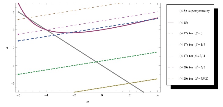
with the help of (4.10) and (4.14), thus providing a linear relation between mm and nn which parametrically depends on β\beta. Plotting in the m​nmn plane the two curves corresponding to (4.15) and (4.17), it is easy to see that they intersect for 2β−1∉]−43,49[2\beta{-}1\notin\ ]{-}{\textstyle\frac{4}{3}},{\textstyle\frac{4}{9}}[\ .66 6 The notation ]a,b[]a,b[ to denote open intervals, to distinguish from pairs (a,b)(a,b). However, since 2​β−1∼ρ>02\beta{-}1\sim\rho>0, we are left with the condition

2​β−1≥49orβ=0andλ2≥139.2\beta-1\ \geq\ {\textstyle\frac{4}{9}}\qquad\text{or}\qquad\beta=0\quad\text{and}\quad\lambda^{2}\ \geq\ {\textstyle\frac{13}{9}}. (4.18)

Consulting the table in the previous section, this rules out the SU(2)3/SU(2)\text{SU(2)}^{3}/\text{SU(2)} case and enforces the choice of F=λ​R−|𝔪F=\lambda R^{-}\big|_{\mathfrak{m}} with a real scaling parameter λ\lambda in the SU(3)/U(1)×U(1)\text{SU(3)}/\text{U(1)}{\times}\text{U(1)} case, as in [9].

Refer to caption
Figure 1: Plot in the mn plane of the curves corresponding to equations (4.5), (4.15), (4.17) (for special values of β\beta) and (4.20) (for special values of λ\lambda).

Let us examine whether a supersymmetric solution is possible. This means that apart from (4.14) and (4.17) we also have to impose the condition (4.5). The corresponding straight line always intersects with the one from (4.17) and meets the curve from (4.14) in the two points (see Figure 1)

(m,n| 2​β−1)=(−4,0|23)and(m,n| 2​β−1)=(−163,43|2827),(m,n\,|\,2\beta{-}1)=(-4,0\,|\,{\textstyle\frac{2}{3}})\qquad\text{and}\qquad(m,n\,|\,2\beta{-}1)=(-{\textstyle\frac{16}{3}},{\textstyle\frac{4}{3}}\,|\,{\textstyle\frac{28}{27}}), (4.19)

both for the lower sign in front of the square root in (4.15). Since those β\beta values do not appear in table (3.16), one may try to obtain a solution for SU(3)/U(1)×U(1)\text{SU(3)}/\text{U(1)}{\times}\text{U(1)} with F=λ​R−|𝔪F=\lambda R^{-}\big|_{\mathfrak{m}}. Replacing 2​β−12\beta{-}1 with λ2−1\lambda^{2}{-}1, we obtain λ2=53\lambda^{2}={\textstyle\frac{5}{3}} and λ2=5527\lambda^{2}={\textstyle\frac{55}{27}}, which are both within the bound (4.18) for β=0\beta=0. Using (4.10), the scales come out as ρ=α′6\rho={\textstyle\frac{\alpha^{\prime}}{6}} and ρ=7​α′27\rho={\textstyle\frac{7\alpha^{\prime}}{27}}, respectively. For a supersymmetric solution, these scales should agree with the condition (4.9), which is equivalent to the vanishing of the external gravitino variation. It is readily observed that this is indeed the case for the first solution, whereas the second one does not satisfy (4.9). The first solution corresponds to Σ=−4​H\Sigma=-4H and vanishing dilatino and was already obtained in [9]. The second one is not a supersymmetric solution. Therefore we conclude that even with a dilatino condensate it is not possible to obtain more than one supersymmetric solution which satisfies all the equations of motion.

Let us now examine the case of non-supersymmetric solutions. This means that we do not have to impose (4.5) or any other condition originating from supersymmetry, leaving more freedom in the problem. We already saw that for any value of β≥1318\beta\geq{\textstyle\frac{13}{18}} as well as for β=0\beta{=}0 at any value of λ2≥139\lambda^{2}\geq{\textstyle\frac{13}{9}} there is a joint solution to (4.14) and (4.17), with a scale ρ=α′4​(2​β−1)≥α′9\rho={\textstyle\frac{\alpha^{\prime}}{4}}(2\beta{-}1)\geq{\textstyle\frac{\alpha^{\prime}}{9}}. Let us perform a case-by-case analysis for the occurring values of β\beta:

  • •

    For β=0\beta=0, we must choose F=λ​R−|𝔪F=\lambda R^{-}\big|_{\mathfrak{m}} and obtain

    λ2−1=118​(4​n−m+8)⟹m−4​n= 26−18​λ2.\lambda^{2}-1\ =\ {\textstyle\frac{1}{18}}(4n-m+8)\quad\Longrightarrow\quad m-4n\ =\ 26-18\lambda^{2}. (4.20)

    This equation combined with (4.15) leads to an infinity of possible solutions parametrized by λ\lambda. Indeed, we find

    m\displaystyle m\!\! =\displaystyle= −13+ 9​λ2±3​27​λ4−30​λ2−13,\displaystyle\!\!-13+\ 9\,\lambda^{2}\pm\sqrt{3}\sqrt{27\lambda^{4}-30\lambda^{2}-13}, (4.21)
    4​n\displaystyle 4n\!\! =\displaystyle= −39+27​λ2±3​27​λ4−30​λ2−13.\displaystyle\!\!-39+27\lambda^{2}\pm\sqrt{3}\sqrt{27\lambda^{4}-30\lambda^{2}-13}. (4.22)

    A direct observation is that for the borderline value of λ2=139\lambda^{2}={\textstyle\frac{13}{9}} we obtain m=0m{=}0 and n=0n{=}0. This is exactly the non-supersymmetric solution with vanishing gaugino and dilatino, which was found in [9]. Moreover, for the special values of λ2=53\lambda^{2}={\textstyle\frac{5}{3}} and λ2=5527\lambda^{2}={\textstyle\frac{55}{27}} we reproduce the supersymmetric and non-supersymmetric solutions discussed earlier. However, here there are obviously more possibilities since any other value of λ2≥139\lambda^{2}\geq{\textstyle\frac{13}{9}} yields a non-supersymmetric solution, giving us an infinite family on SU(3)/U(1)×U(1)\text{SU(3)}/\text{U(1)}{\times}\text{U(1)}.

  • •

    For β=34\beta={\textstyle\frac{3}{4}}, we obtain

    m−4​n=−1,m-4n=-1, (4.23)

    which, combined with (4.15), leads to the values

    (m,n)=(12​(1±33),18​(3±33)).(m,n)=\big({\textstyle\frac{1}{2}}(1\pm\sqrt{33}),{\textstyle\frac{1}{8}}(3\pm\sqrt{33})\big). (4.24)

    Then we also find that ρ=α′8\rho={\textstyle\frac{\alpha^{\prime}}{8}}, which is a legitimate solution.

  • •

    For β=13\beta={\textstyle\frac{1}{3}}, we land outside the admissible range, as discussed above.

  • •

    There is a fourth case corresponding to the manifold Sp(2)/Sp(1)×U(1)\text{Sp(2)}/\text{Sp(1)}{\times}\text{U(1)}, where there is no common value for β\beta. Instead, we have β=0\beta=0 on 𝔲⁡(1)\mathfrak{u}(1) and β=23\beta={\textstyle\frac{2}{3}} on 𝔰​𝔭​(1)\mathfrak{sp}(1). This allows one to calculate the quantities tr(R±∧R±)(R^{\pm}\wedge R^{\pm}), which are no longer proportional to d​HdH. However, we have the freedom to restrict the curvature R~\tilde{R} to the 𝔲⁡(1)\mathfrak{u}(1) part of 𝔥\mathfrak{h}. Again this can be rescaled, enabling us to satisfy the Bianchi identity for a particular choice,

    R~=R|𝔲⁡(1)andF=R−|𝔪⟹tr​(R~∧R~−F∧F)=13​ρ−1​d​H.\tilde{R}=R\big|_{\mathfrak{u}(1)}\qquad\text{and}\qquad F\ =\ R^{-}\big|_{\mathfrak{m}}\qquad\Longrightarrow\qquad\text{tr}(\tilde{R}\wedge\tilde{R}-F\wedge F)\ =\ {\textstyle\frac{1}{3}}\,\rho^{-1}dH. (4.25)

    In contrast to the SU(3)/U(1)×\timesU(1) case, there are then no free parameters left in the gauge field. Moreover,

    tr​(|R~|2−|F|2)=−13​ρ2.\text{tr}(|\tilde{R}|^{2}-|F|^{2})\ =\ -{\textstyle\frac{1}{3\rho^{2}}}. (4.26)

    Then, according to the above, we end up with the condition

    m−4​n= 2,m-4n\ =\ 2, (4.27)

    which however has no intersection with (4.14). Hence, although we find that ρ=α′12>0\rho={\textstyle\frac{\alpha^{\prime}}{12}}>0, there is no solution on Sp(2)/Sp(1)×U(1)\text{Sp(2)}/\text{Sp(1)}{\times}\text{U(1)}.

Scan for solutions with 𝚪~=𝚪+\mathbf{\tilde{\Gamma}=\Gamma^{+}}.

Let us continue by choosing R~=R+\tilde{R}=R^{+}, which is not an instanton. For FF we insist on the previous choice, i.e. FF is still chosen to be an instanton gauge field. In that case (4.12) and (4.11) yield, respectively,

2​β\displaystyle 2\beta\!\! =\displaystyle{=} 4​ρα′=136​(14​m2−12​m​n−m+4​n+16),\displaystyle\!\!4{\textstyle\frac{\rho}{\alpha^{\prime}}}\ =\ {\textstyle\frac{1}{36}}({\textstyle\frac{1}{4}}m^{2}-{\textstyle\frac{1}{2}}mn-m+4n+16), (4.28)
43−2​β\displaystyle{\textstyle\frac{4}{3}}-2\beta\!\! =\displaystyle{=} −ρ3​α′​(14​m2−12​m​n+m−4​n+12).\displaystyle\qquad-{\textstyle\frac{\rho}{3\alpha^{\prime}}}({\textstyle\frac{1}{4}}m^{2}-{\textstyle\frac{1}{2}}mn+m-4n+12). (4.29)

Let us again perform a case-by-case analysis for the occurring values of β\beta.

  • •

    For β=0\beta=0, in the present case it is obvious that we are immediately led to ρ=0\rho=0, which is not acceptable. However, as we discussed before, one may try to obtain solutions for the rescaled connection F=λ​R−|𝔪F=\lambda R^{-}|_{\mathfrak{m}}. Presently such a choice leads to the replacement of 2​β2\beta in (4.28) and (4.29) by λ2\lambda^{2}. Then (4.28) requires that λ2∼ρ>0\lambda^{2}\sim\rho>0, which is true since λ∈ℝ\lambda\in\mathbb{R}. Solving the two equations we obtain the following result,

    m\displaystyle m\!\! =\displaystyle{=} −4+ 9​λ2+λ−2​(  4±16−96​λ2+24​λ4+72​λ6+81​λ8),\displaystyle\,-4+\ 9\,\lambda^{2}+\lambda^{-2}\bigl(\ \;4\pm\sqrt{16-96\lambda^{2}+24\lambda^{4}+72\lambda^{6}+81\lambda^{8}}\bigr), (4.30)
    4​n\displaystyle 4n\!\! =\displaystyle{=} −12+27​λ2+λ−2​(12±16−96​λ2+24​λ4+72​λ6+81​λ8),\displaystyle\!\!-12+27\lambda^{2}+\lambda^{-2}\bigl(12\pm\sqrt{16-96\lambda^{2}+24\lambda^{4}+72\lambda^{6}+81\lambda^{8}}\bigr), (4.31)

    under the condition that |λ||\lambda| lies in the domain 77 7 The interval border value 0.4240.424 approximates the positive root of the polynomial equation 27​λ6+42​λ4+36​λ2−8=027\lambda^{6}+42\lambda^{4}+36\lambda^{2}-8=0; the other border value is 13​6≈0.816{\textstyle\frac{1}{3}}\sqrt{6}\approx 0.816 .

    |λ|∈]0,0.424[∪]0.8816,∞[.|\lambda|\,\in\,\ ]0\,,0.424[\ \cup\ ]0.8816\,,\infty[\ . (4.32)

    Therefore we obtain again a infinite family of solutions on SU(3)/U(1)×U(1)\text{SU(3)}/\text{U(1)}{\times}\text{U(1)}.

    It is interesting to observe that the parameter nn does not vanish for any of the allowed values of λ\lambda. This is in accord with the results of [9]. However, for the value λ2=29​(1+10)\lambda^{2}={\textstyle\frac{2}{9}}(1+\sqrt{10}), which lies in the allowed domain, the parameter mm vanishes. Then this solution corresponds to vanishing gaugino but non-vanishing dilatino condensate.

  • •

    For β=34\beta={\textstyle\frac{3}{4}}, the first of the above equations yields ρ=38​α′\rho={\textstyle\frac{3}{8}}\alpha^{\prime}, which is positive as required. Then we can proceed to the solutions for mm and nn. We find

    m\displaystyle m\!\! =\displaystyle{=} 16​(  73±9265)≈ 12.167±16.042,\displaystyle\!\!{\textstyle\frac{1}{6}}\big(\ \,73\pm\sqrt{9265}\big)\ \approx\ 12.167\pm 16.042, (4.33)
    4​n\displaystyle 4n\!\! =\displaystyle{=} 16​(219±9265)≈ 36.500±16.042.\displaystyle\!\!{\textstyle\frac{1}{6}}\big(219\pm\sqrt{9265}\big)\ \approx\ 36.500\pm 16.042. (4.34)

    These values provide two solutions on G2/SU(3)G_{2}/\text{SU(3)} for the plus-connection.

  • •

    For β=13\beta={\textstyle\frac{1}{3}}, we obtain ρ=α′6>0\rho={\textstyle\frac{\alpha^{\prime}}{6}}>0. Moreover, solving the two equations for mm and nn we arrive at

    (m,n)=(8,6),(m,n)=(8,6), (4.35)

    which corresponds to a solution on SU(2)3/SU(2)\text{SU(2)}^{3}/\text{SU(2)} for the plus-connection.

  • •

    As far as the space Sp(2)/Sp(1)×U(1)\text{Sp(2)}/\text{Sp(1)}{\times}\text{U(1)} is concerned, unlike the Γ−\Gamma^{-} case where the connection is an 𝔥\mathfrak{h}-gauge field and therefore the curvature can be restricted to the 𝔲⁡(1)\mathfrak{u}(1) part of 𝔥\mathfrak{h}, this freedom does not exist here. Therefore it is not possible to satisfy the Bianchi identity on this space with the plus-connection.

Let us note that none of the solutions with plus-connection is supersymmetric since they all fail to satisfy the condition (4.5).

The remaining equations of motion and fermion masses.

Let us finish this section by commenting on the equations of motion which were not treated in detail until now. These are the Einstein equation, the gaugino and dilatino equations of motion, the Yang-Mills equation and the Kalb-Ramond equation, all appearing in (2.33).

As far as the (internal) Einstein equation is concerned, all its terms are proportional to ga​bg_{ab},88 8 For our choice of η\eta being an internal Killing spinor, the right-hand side of the third equation in (2.33) vanishes identically. and therefore it is enough to solve its trace. However, the trace is identical to (4.11), which was already taken into account. Therefore the Einstein equation on KK is satisfied.

The Yang-Mills equation of motion is also satisfied since in the above analysis we assumed that the gauge field is always an instanton. As for the Kalb-Ramond equation, since Σ\Sigma and Δ\Delta are both proportional to HH it is simplified to

d∗H=0.d\ast H=0. (4.36)

Then this is satisfied due to the relations (3.2), (3.7) and (3.3).

Finally, let us turn to the Dirac equations for the gaugino and the dilatino. We have already considered the decomposition of the corresponding spinors in terms of the spinor η\eta on the internal space in (2.20) and (2.22). Moreover, we know that the spinor η\eta is covariantly constant with respect to the torsionful connection ∇−\nabla^{-}, thus

𝒟−​η=0⟹(𝒟−18​γ​(H))​η=0,\mathcal{D}^{-}\eta=0\qquad\Longrightarrow\qquad\big(\mathcal{D}-{\textstyle\frac{1}{8}}\gamma(H)\big)\,\eta=0, (4.37)

and likewise for η∗\eta^{\ast}. The above indicate that it is useful to express the gaugino and dilatino equations in terms of 𝒟−{\mathcal{D}}^{-}. We obtain

=\displaystyle= (𝒟^+𝒟−+124​γ​(2​H+12​Σ−12​Δ))​χ=(𝒟^+148​(4+m−n)​γ​(H))​χ,\displaystyle\!\!\big(\widehat{\mathcal{D}}+\mathcal{D}^{-}+{\textstyle\frac{1}{24}}\gamma(2H+{\textstyle\frac{1}{2}}\Sigma-{\textstyle\frac{1}{2}}\Delta)\big)\,\chi\ =\ \big(\widehat{\mathcal{D}}+{\textstyle\frac{1}{48}}(4{+}m{-}n)\gamma(H)\big)\,\chi, (4.38)
=\displaystyle= (𝒟^+𝒟−+124​γ​(2​H+18​Σ))​λ=(𝒟^+148​(4+14​m)​γ​(H))​λ.\displaystyle\!\!\big(\widehat{\mathcal{D}}+\mathcal{D}^{-}+{\textstyle\frac{1}{24}}\gamma(2H+{\textstyle\frac{1}{8}}\Sigma)\big)\,\lambda\qquad\quad\!\ =\ \big(\widehat{\mathcal{D}}+{\textstyle\frac{1}{48}}(4{+}{\textstyle\frac{1}{4}}m)\gamma(H)\big)\,\lambda. (4.39)

After computing

γ⁡(H)​(ei​π4​χ^⊗η+e−i​π4​χ^∗⊗η∗)\displaystyle\gamma(H)\,\big(e^{\frac{i\pi}{4}}\widehat{\chi}{\otimes}\eta+e^{-\frac{i\pi}{4}}\widehat{\chi}^{\ast}{\otimes}\eta^{\ast}\big)\!\! =\displaystyle= −123​ρ​(e−i​π4​χ^⊗η∗+ei​π4​χ^∗⊗η),\displaystyle\!\!-{\textstyle\frac{12}{\sqrt{3\rho}}}\big(e^{-\frac{i\pi}{4}}\widehat{\chi}{\otimes}\eta^{\ast}+e^{\frac{i\pi}{4}}\widehat{\chi}^{\ast}{\otimes}\eta\big), (4.40)
γ⁡(H)​(ei​π4​λ^⊗η∗+e−i​π4​λ^∗⊗η)\displaystyle\gamma(H)\,\big(e^{\frac{i\pi}{4}}\widehat{\lambda}{\otimes}\eta^{\ast}+e^{-\frac{i\pi}{4}}\widehat{\lambda}^{\ast}{\otimes}\eta\big)\!\! =\displaystyle= −123​ρ​(e−i​π4​λ^⊗η+ei​π4​λ^∗⊗η∗),\displaystyle\!\!-{\textstyle\frac{12}{\sqrt{3\rho}}}\big(e^{-\frac{i\pi}{4}}\widehat{\lambda}{\otimes}\eta+e^{\frac{i\pi}{4}}\widehat{\lambda}^{\ast}{\otimes}\eta^{\ast}\big), (4.41)

the vanishing of the coefficients of η\eta and η∗\eta^{\ast} in (4.38) and (4.39) yields massive Dirac equations on AdS4,99 9 Note that no imaginary unit appears here because of our sign choice in the Clifford algebra (2.18).

𝒟^​χ^=mχ​χ^∗and𝒟^​λ^=mλ​λ^∗,\widehat{\mathcal{D}}\,\widehat{\chi}\ =\ m_{\chi}\,\widehat{\chi}^{\ast}\qquad\text{and}\qquad\widehat{\mathcal{D}}\,\widehat{\lambda}\ =\ m_{\lambda}\,\widehat{\lambda}^{\ast}, (4.42)

with four-dimensional gaugino and dilatino masses given by

mχ=4+m−n4​3​ρandmλ=16+m16​3​ρ.m_{\chi}\ =\ \frac{4{+}m{-}n}{4\sqrt{3\rho}}\qquad\text{and}\qquad m_{\lambda}\ =\ \frac{16{+}m}{16\sqrt{3\rho}}. (4.43)

With the help of (4.10) one may express the scale ρ\rho in terms of α′\alpha^{\prime} for each case of values (m,n)(m,n). A similar formula was determined in [21] for a general choice of connection. In the following section, where we summarize our results, we shall provide the explicit masses in terms of the string slope α′\alpha^{\prime}.

5 Summary of results and discussion

In this paper we examined AdS4 heterotic compactifications on nearly Kähler manifolds with non-vanishing gaugino and dilatino bilinears. We were able to find a set of solutions with properties which are summarized in the following three tables. In the first table appear the common features of all the solutions we found:

quantity symbol value
AdS radius rr α′2\sqrt{{\textstyle\frac{\alpha^{\prime}}{2}}}
HH-flux Ha​b​cH_{abc} −fa​b​c-f_{abc}
dilaton vev ϕ\phi constant
10​d10d gaugino χ\chi ei​π4​χ^⊗η+e−i​π4​χ^∗⊗η∗e^{\frac{i\pi}{4}}\widehat{\chi}\otimes\eta+e^{-\frac{i\pi}{4}}\widehat{\chi}^{*}\otimes\eta^{*}
10​d10d dilatino λ\lambda ei​π4​λ^⊗η∗+e−i​π4​λ^∗⊗ηe^{\frac{i\pi}{4}}\widehat{\lambda}\otimes\eta^{\ast}+e^{-\frac{i\pi}{4}}\widehat{\lambda}^{\ast}\otimes\eta
10​d10d gravitino ψ\psi 0

In the second table we list some solution-dependent features for the five (sets of) solutions determined:

internal space internal scale ρ\rho metric ga​bg_{ab} connection Γ~\tilde{\Gamma} gauge field Fa​bF_{ab}
1 SU(3)/U(1)×U(1)\text{SU(3)}/\text{U(1)}{\times}\text{U(1)} (λ2−1)​α′4(\lambda^{2}-1){\textstyle\frac{\alpha^{\prime}}{4}} (1−λ2)​3​α′4​fa​dc​fb​cd(1-\lambda^{2}){\textstyle\frac{3\alpha^{\prime}}{4}}f^{c}_{ad}f^{d}_{bc} Γ−\Gamma^{-} λ​Ra​b−|𝔪\lambda R_{ab}^{-}|_{\mathfrak{m}}
2 G2/SU(3)G_{2}/\text{SU(3)} α′8{\textstyle\frac{\alpha^{\prime}}{8}} −3​α′8​fa​dc​fb​cd-{\textstyle\frac{3\alpha^{\prime}}{8}}f^{c}_{ad}f^{d}_{bc} Γ−\Gamma^{-} Ra​b−|𝔥R_{ab}^{-}|_{\mathfrak{h}}
3 SU(3)/U(1)×U(1)\text{SU(3)}/\text{U(1)}{\times}\text{U(1)} λ2​α′4\lambda^{2}{\textstyle\frac{\alpha^{\prime}}{4}} −λ2​3​α′4​fa​dc​fb​cd-\lambda^{2}{\textstyle\frac{3\alpha^{\prime}}{4}}f^{c}_{ad}f^{d}_{bc} Γ+\Gamma^{+} λ​Ra​b−|𝔪\lambda R_{ab}^{-}|_{\mathfrak{m}}
4 G2/SU(3)G_{2}/\text{SU(3)} 3​α′8{\textstyle\frac{3\alpha^{\prime}}{8}} −9​α′8​fa​dc​fb​cd-{\textstyle\frac{9\alpha^{\prime}}{8}}f^{c}_{ad}f^{d}_{bc} Γ+\Gamma^{+} Ra​b−|𝔥R_{ab}^{-}|_{\mathfrak{h}}
5 SU(2)3/SU(2)\text{SU(2)}^{3}/\text{SU(2)} α′6{\textstyle\frac{\alpha^{\prime}}{6}} −α′2​fa​dc​fb​cd-{\textstyle\frac{\alpha^{\prime}}{2}}f^{c}_{ad}f^{d}_{bc} Γ+\Gamma^{+} Ra​b−|𝔥R_{ab}^{-}|_{\mathfrak{h}}

For the first solution the allowed domain for λ\lambda is λ2≥139\lambda^{2}\geq{\textstyle\frac{13}{9}}, while for the third solution it is λ2≥23\lambda^{2}\geq{\textstyle\frac{2}{3}} or λ2≤0.18,λ≠0\lambda^{2}\leq 0.18,~\lambda\neq 0. Finally, the remaining solution properties are given in the third table:

bilinear values (m,n)(m,n) gaugino mass2 mχ2m^{2}_{\chi} dilatino mass2 mλ2m^{2}_{\lambda}
1 (−13+9​λ2±P⁡(λ2),14​(−39+27​λ2±P⁡(λ2)))\big(-13+9\lambda^{2}\pm P(\lambda^{2}),{\textstyle\frac{1}{4}}(-39+27\lambda^{2}\pm P(\lambda^{2}))\big) 3​(1+3​λ2±P⁡(λ2))264​α′​(λ2−1){\textstyle\frac{3(1+3\lambda^{2}\pm P(\lambda^{2}))^{2}}{64\alpha^{\prime}(\lambda^{2}-1)}} (3+9​λ2±P⁡(λ2))2192​α′​(λ2−1){\textstyle\frac{(3+9\lambda^{2}\pm P(\lambda^{2}))^{2}}{192\alpha^{\prime}(\lambda^{2}-1)}}
2 (12​(1±33),18​(3±33))\big({\textstyle\frac{1}{2}}(1\pm\sqrt{33}),{\textstyle\frac{1}{8}}(3\pm\sqrt{33})\big) 3364​α′​(7±33){\textstyle\frac{33}{64\alpha^{\prime}}}(7\pm\sqrt{33}) 1164​α′​(17±33){\textstyle\frac{11}{64\alpha^{\prime}}}(17\pm\sqrt{33})
3 (−4+9​λ2+4±Q⁡(λ2)λ2,−3+274​λ2+3±14​Q​(λ2)λ2)\big(-4+9\lambda^{2}+\frac{4\pm Q(\lambda^{2})}{\lambda^{2}},-3+{\textstyle\frac{27}{4}}\lambda^{2}+\frac{3\pm{\textstyle\frac{1}{4}}Q(\lambda^{2})}{\lambda^{2}}\big) (4+12​λ2+9​λ4±3​Q​(λ2))2192​λ6​α′{\textstyle\frac{(4+12\lambda^{2}+9\lambda^{4}\pm 3Q(\lambda^{2}))^{2}}{192\lambda^{6}\alpha^{\prime}}} (4+12​λ2+9​λ4±Q⁡(λ2))2192​λ6​α′{\textstyle\frac{(4+12\lambda^{2}+9\lambda^{4}\pm Q(\lambda^{2}))^{2}}{192\lambda^{6}\alpha^{\prime}}}
4 (16​(73±9265,124​(219±9265)CLOSECLOSE\big({\textstyle\frac{1}{6}}\big(73\pm\sqrt{9265},{\textstyle\frac{1}{24}}\big(219\pm\sqrt{9265}\big) 55973±507​92655184​α′{\textstyle\frac{55973\pm 507\sqrt{9265}}{5184\alpha^{\prime}}} (169±9265)210368​α′{\textstyle\frac{(169\pm\sqrt{9265})^{2}}{10368\alpha^{\prime}}}
5 (8,6)(8,6) 92​α′{\textstyle\frac{9}{2\alpha^{\prime}}} 92​α′{\textstyle\frac{9}{2\alpha^{\prime}}}

with  P⁡(λ2)=3​27​λ4−30​λ2−13P(\lambda^{2})=\sqrt{3}\sqrt{27\lambda^{4}-30\lambda^{2}-13}  and  Q⁡(λ2)=16−96​λ2+24​λ4+72​λ6+81​λ8Q(\lambda^{2})=\sqrt{16-96\lambda^{2}+24\lambda^{4}+72\lambda^{6}+81\lambda^{8}} .

Let us moreover note that all the above solutions are non-supersymmetric, except for the first solution on SU(3)/U(1)×U(1)\text{SU(3)}/\text{U(1)}\times\text{U(1)} with the special value λ2=53\lambda^{2}={\textstyle\frac{5}{3}} and the lower sign, yielding (m,n)=(−4,0)(m,n)=(-4,0), P⁡(53)=6P({\textstyle\frac{5}{3}})=6 and (mχ2,mλ2)=(0,98​α′)(m^{2}_{\chi},m^{2}_{\lambda})=(0,{\textstyle\frac{9}{8\alpha^{\prime}}}).

Having summarized our findings let us discuss some interesting aspects of the above solutions. The first message is that, for heterotic compactifications on SU(3) structure manifolds, the Killing spinor equations and the Bianchi identity do not imply the equations of motion. The only two exceptions are the well-known Calabi-Yau case of vanishing HH-flux and connection Γ−\Gamma^{-} and the first (and only supersymmetric) solution in the above tables on SU(3)/U(1)×U(1)\text{SU(3)}/\text{U(1)}{\times}\text{U(1)} again with connection Γ−\Gamma^{-} and λ2=53\lambda^{2}={\textstyle\frac{5}{3}}. The latter corresponds to vanishing dilatino condensate but non-vanishing HH-flux and gaugino condensate. Turning on a non-vanishing dilatino condensate does not improve the situation drastically from the point of view of supersymmetric vacua. Indeed, it turns out that it does not lead to any new supersymmetric solution. Thus although it provides an extra freedom to solve the Killing spinor equations and the Bianchi identity [7], this freedom is lost at the level of the equations of motion.

It goes without saying that the equations of motion and the absence of anomalies are more fundamental than the supersymmetry equations. Therefore, in the present paper we worked at the level of the equations of motion and the Bianchi identity at first order in α′\alpha^{\prime}, allowing for non-vanishing supersymmetry variations. 1010 10 It is worth mentioning that non-supersymmetric Minkowski compactifications with non-vanishing fermion bilinears were considered recently in the context of 11d supergravity [22]. Our basic assumptions were threefold: (1) the HH-flux is identified with the torsion of the internal space, (2) the gauge field is a generalized instanton 1111 11 This assumption facilitates the solution of the Yang-Mills equations. However, different assumptions for the gauge field are fully legitimate as long as the corresponding equations are satisfied. Different choices for the gauge field appear for example in [23], where however the equations of motion are not checked explicitly. and (3) gaugino and dilatino bilinears may develop a vacuum expectation value. It is interesting that under these assumptions it was possible to fully classify the consistent vacua of the theory on nearly Kähler manifolds, regardless of their remnant supersymmetry. This examination resulted in the solutions appearing in the above tables. The introduction of a dilatino condensate clearly brings up more solutions than before, albeit non-supersymmetric ones.

A further interesting issue is that all our solutions fix the radius of AdS4 as well as the volume modulus ρ\rho of the internal nearly Kähler space. This provides a partial moduli stabilization in four dimensions. As far as the rest of the moduli are concerned, i.e. the four-dimensional dilaton and the Kähler moduli of the compactification, their stabilization may be studied within the effective scalar potential in the four-dimensional theory. This potential was partially determined for nearly Kähler manifolds in [24, 25] in the absence of fermion condensates. The presence of fermion condensates typically leads to an effective component in the four-dimensional superpotential, which is known at least for the gaugino condensates [3, 4]. This effective superpotential may assist the stabilization of the dilaton in four dimensions [26].

Since generically supersymmetry is broken, the gaugino and the dilatino acquire non-vanishing masses. These masses depend on the internal geometry and are calculable as we have demonstrated. It is worth noting that in the single supersymmetric case on SU(3)/U(1)×U(1)\text{SU(3)}/\text{U(1)}{\times}\text{U(1)} the gaugino mass vanishes, as expected, while the dilatino mass squares to mλ2=98​α′m^{2}_{\lambda}={\textstyle\frac{9}{8\alpha^{\prime}}}. As a potentially interesting feature of our analysis, the stabilization of the internal scale allows one to calculate the fermion masses explicitly in terms of the string scale.

Acknowledgments.

This work was partially supported by the Deutsche Forschungsgemeinschaft, the cluster of excellence QUEST, the Heisenberg-Landau program, the Russian Foundation for Basic Research, the SFB-Tansregio TR33 “The Dark Universe” (Deutsche Forschungsgemeinschaft) and the European Union 7th network program “Unification in the LHC era” (PITN-GA-2009-237920).

References

  • [1] A. Strominger, Nucl. Phys. B 274 (1986) 253.
  • [2] G. Lopes Cardoso, G. Curio, G. Dall’Agata, D. Lüst, P. Manousselis and G. Zoupanos,
    Nucl. Phys. B 652 (2003) 5 [hep-th/0211118].
  • [3] M. Dine, R. Rohm, N. Seiberg and E. Witten, Phys. Lett. B 156 (1985) 55.
  • [4] J.P. Derendinger, L.E. Ibanez and H.P. Nilles, Phys. Lett. B 155 (1985) 65.
  • [5] G. Lopes Cardoso, G. Curio, G. Dall’Agata and D. Lüst, Fortsch. Phys. 52 (2004) 483 [hep-th/0310021].
  • [6] A.R. Frey and M. Lippert, Phys. Rev. D 72 (2005) 126001 [hep-th/0507202].
  • [7] P. Manousselis, N. Prezas and G. Zoupanos, Nucl. Phys. B 739 (2006) 85 [hep-th/0511122].
  • [8] S. Ivanov, Phys. Lett. B 685 (2010) 190 [arXiv:0908.2927 [hep-th]].
  • [9] O. Lechtenfeld, C. Nölle and A.D. Popov, JHEP 1009 (2010) 074 [arXiv:1007.0236 [hep-th]].
  • [10] E. Bergshoeff, M. de Roo, B. de Wit and P. van Nieuwenhuizen, Nucl. Phys. B 195 (1982) 97.
  • [11] G.F. Chapline and N.S. Manton, Phys. Lett. B 120 (1983) 105.
  • [12] E.A. Bergshoeff and M. de Roo, Nucl. Phys. B 328 (1989) 439.
  • [13] K. Becker and S. Sethi, Nucl. Phys. B 820 (2009) 1 [arXiv:0903.3769 [hep-th]].
  • [14] M. Graña, Phys. Rept. 423 (2006) 91 [hep-th/0509003].
  • [15] S.R. Green, E.J. Martinec, C. Quigley and S. Sethi,
    Class. Quant. Grav. 29 (2012) 075006 [arXiv:1110.0545 [hep-th]].
  • [16] J.-B. Butruille, Homogeneous nearly Kähler manifolds, arXiv:math/0612655.
  • [17] L. Castellani, L.J. Romans and N.P. Warner, Annals Phys. 157 (1984) 394.
  • [18] F. Müller-Hoissen and R. Stuckl, Class. Quant. Grav. 5 (1988) 27.
  • [19] A.D. Popov, Nucl. Phys. B 828 (2010) 594 [arXiv:0907.0106 [hep-th]].
  • [20] H. Baum, Twistor spinors on Lorentzian symmetric spaces, arXiv:math/9803089.
  • [21] P. Manousselis and G. Zoupanos, JHEP 0203 (2002) 002 [hep-ph/0111125].
  • [22] F. Farakos, A. Kehagias and E.N. Saridakis, JHEP 1112 (2011) 107 [arXiv:1111.1577 [hep-th]].
  • [23] M. Klaput, A. Lukas and C. Matti, JHEP 1109 (2011) 100 [arXiv:1107.3573 [hep-th]].
  • [24] A. Chatzistavrakidis, P. Manousselis and G. Zoupanos,
    Fortsch. Phys. 57 (2009) 527 [arXiv:0811.2182 [hep-th]].
  • [25] A. Chatzistavrakidis and G. Zoupanos, JHEP 0909 (2009) 077 [arXiv:0905.2398 [hep-th]].
  • [26] B. de Carlos, S. Gurrieri, A. Lukas and A. Micu, JHEP 0603 (2006) 005 [hep-th/0507173].